Power Flow as Intersection of Circles:
A New Fixed Point Method

Abstract

The power flow (PF) problem is a fundamental problem in power system engineering. Many popular solvers face challenges, such as convergence issues. One can try to rewrite the PF problem into a fixed point equation, which can be solved exponentially fast. But, existing methods have their own restrictions, such as the required AC network structure or bus types. To remove these restrictions, we employ the circle geometry per-bus via rectangular coordinate representation to embed our physical knowledge of operation point selection in PV curves. Each iteration of the algorithm consists of finding intersections of circles, which can be computed efficiently with high numerical accuracy. Such analysis also helps in visualizing PV curve to always select the high voltage solution. We compare the performance of our fixed point algorithm with existing state-of-the-art methods, showing that the proposed method can correctly find the solutions when other methods cannot. In addition, we empirically show that the fixed point algorithm is much more robust to bad initialization points than the existing methods.

I Introduction

The power flow problem is one of the canonical problems in power engineering and it is frequently used in power system operation and planning studies [1, 2]. Existing power flow methods mostly rely on iterative methods such as Newton-Raphson (NR) [3] or fast decoupled load flow (FDLF) [4, 5]. These algorithms have been the workhorses of the power industry and have performed well most of the time. However, as large-scale development of renewable resources and distributed generation push systems to operate in new regimes, the existing algorithms can experience convergence issues, especially when systems operate close to their loadability limits [6, 7, 8]. Therefore, the need for new efficient and robust power flow algorithms to complement these existing methods remains despite decades of studies [9].

Algorithms like NR can be thought as variants of descent algorithms (or approximate descent in the case of FDLF) that modifies the solution iteratively. A fundamental reason for why these algorithms can fail to converge to a solution is simply because the geometry of power flow is not convex [10, 11]. For example, NR uses the Jacobian to find the direction of the steepest descent. Because the power flow equations are nonlinear and nonconvex, there are many local minimums and saddle points, and the Jacobian fails to provide a meaningful descent direction at these points. To prevent the algorithm from getting stuck, it becomes important to pick ”good” initial starting points [12, 13, 14, 15]. Consequently, a number of methods have been developed to overcome the sensitive dependence on the initial guess [16, 17, 18, 19].

As systems start to operate closer to there limits, picking better initialization points becomes insufficient. Since the Jacobians for all points close to the boundary of the feasible power flow region have eigenvalues close to 0 (they loose rank), they necessarily become ill-conditioned and iterative algorithms may diverge [20, 21, 22]. To avoid this phenomenon, a class of non-divergent power flow algorithms was developed to accelerate or decelerate the updates based on the conditioning of the Jacobian [23, 24, 25, 26]. However, these approaches can still be sensitive to the initial guess and sometimes exhibit oscillatory behavior, where the solutions may neither converge nor diverge. An approach using complementarity conditions is developed in [27], but it can reach local minimums or saddle points instead of the true power flow solution. Energy-bases analysis based on mechanical models can help algorithms to escape these stationary points [28], but implementing them for different bus types in a practical power system is non-trivial.

Recently, a new class of power flow formulations based on fixed point equations has been proposed to overcome the algorithmic challenges present in descent algorithms [29, 30]. The basic idea is to write the power flow equations in a form of $\mathbf{v}=f(\mathbf{v})$, where $\mathbf{v}$ is the complex voltage and a fixed point of the function $f$ [31]. If this relationship can be found, then a simple algorithm to find the fixed point is to repeatedly apply the function $f$. Furthermore, if the iterates converge to the fixed point, then it will converge exponentially quickly. The challenge is to find a suitable $f$, which have only exists for restricted class of systems. For example, the results in [30] applies to networks with only PQ buses and the results in [29] only applies to purely inductive (lossless) radial networks.

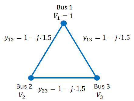
(a) 3-bus system.

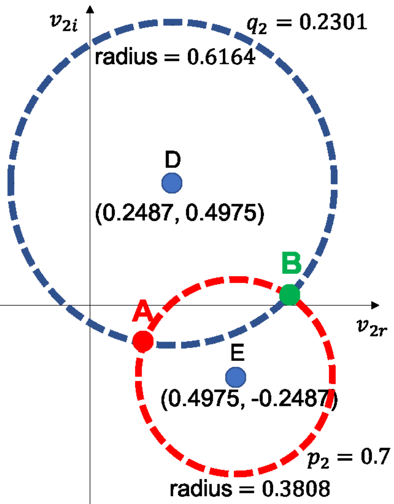
(b) P and Q at bus 2.

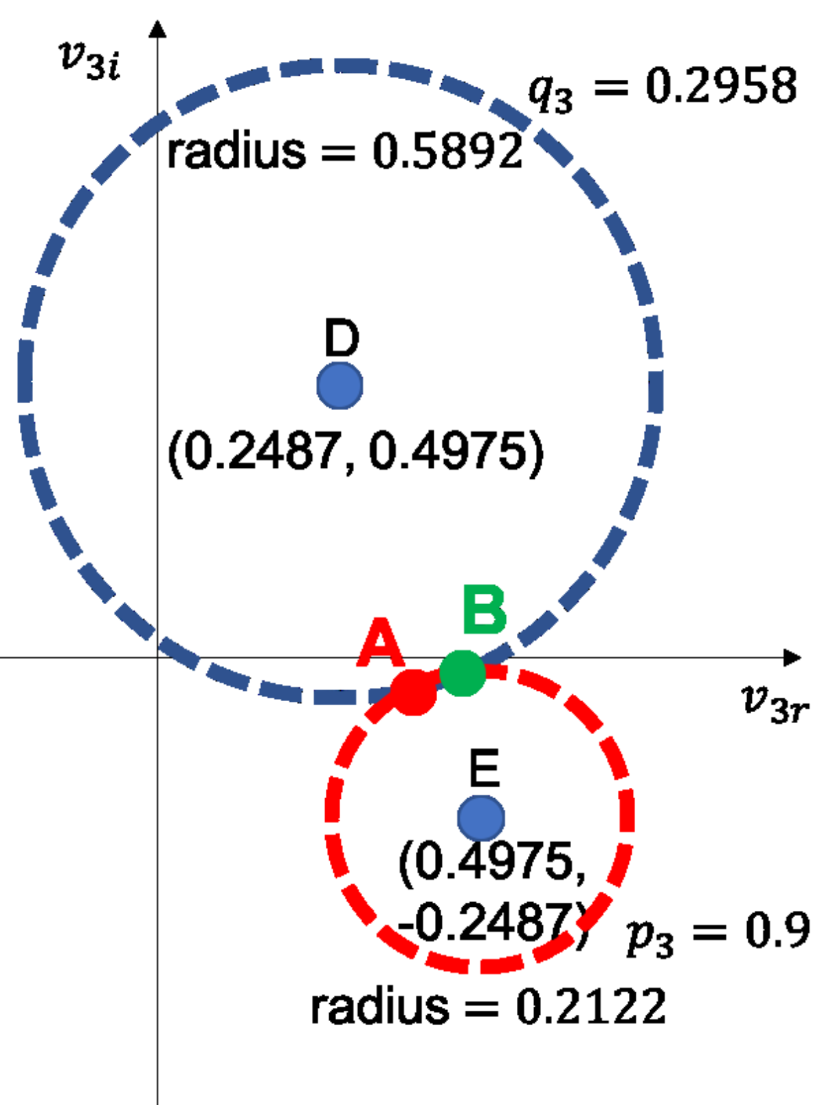
(c) P and Q at bus 3.

Figure 1: Active and reactive circles for a three-bus system. Bus 1 is the slack bus and buses 2 and 3 are PQ buses.

In this paper, we present a novel fixed point formulation of the full AC power flow equations that is applicable to networks with arbitrary topologies and mixture of PQ and PV buses. This approach work is based on a coordinate transformation, where power flow solutions are interpreted as the intersections of circles, where the parameters (center and radius) of the circles depend linearly on the voltages of the neighboring buses. This formulation can be thought as a generalization of the PV noise curve often used to visualize power transfer between two buses. Computationally, only the intersection of two circles needs to be calculated, which involves a series of simple algebraic computations. Therefore, this approach is much cheaper than algorithms (e.g., NR) that require matrix calculations.

To verify the performance of our algorithm, we test it on the standard IEEE systems, including large ones with $2383$ and 3375 buses. We compare our approach with NR, FDLF and non-divergent power flow algorithms. We show that when the loading is heavy, our algorithm is able to converge to the right solution while the other algorithm can diverge or become unstable. In addition, we show that our method is much more robust to random initialization points than the other methods. It is important to note that we are not advocating to replace existing power flow solvers. These algorithms have been highly optimized and do perform extremely well in many situations. Rather, the proposed algorithm in this paper can be used as a complementary tool by the system operators when conventional algorithm diverge or stall.

The paper is organized as follows: Section II introduces the rectangular power flow equations and show how they can be thought as intersections of circles. Section III discusses the fixed point formulation of the power flow equations and walks through a three-bus example. Section IV presents the main algorithm. Section IV-B introduces a $3$-tuple vector form of circles and shows how closed-form formulas with good numerical properties can be found using the vector notation. Section V shows numerical results of our proposed algorithm compared against existing state-of-the-art algorithms on different IEEE benchmark networks. Section VI concludes the paper.

II Power Flow Equations and Circles

II-A Power Flow Equations in Rectangular Coordinates

Throughout this paper we use rectangular coordinates where a bus is index by $d$; $p_{d}$ and $q_{d}$ are the active and reactive powers, respectively; $\mathit{v}_{d,r}$ and $\mathit{v}_{d,i}$ are the real and imaginary parts of the bus voltage, respectively; and $\mathcal{N}(d)$ is the set of neighboring buses connected to bus $d$. We adopt the standard $\Pi$ model of transmission lines [2] and write the admittance of a line between buses $d$ and $k$ as $g_{dk}+jb_{dk}$. We assume that $b_{dk}\leq 0$ for all lines (lines are inductive). In these notations, the power flow equations become [32, 33]:

$$\mathit{p}_{d}=t_{d,1}\cdot\mathit{v}^{2}_{d,r}+t_{d,2}\cdot\mathit{v}_{d,r}+t_{d,1}\cdot\mathit{v}^{2}_{d,i}+t_{d,3}\cdot\mathit{v}_{d,i},$$ (1)

$$\mathit{q}_{d}=t_{d,4}\cdot\mathit{v}^{2}_{d,r}-t_{d,3}\cdot\mathit{v}_{d,r}+t_{d,4}\cdot\mathit{v}^{2}_{d,i}+t_{d,2}\cdot\mathit{v}_{d,i}.$$ (2)

The parameters $t_{d,1},t_{d,2},t_{d,3},t_{d,4}$ are given by

$$t_{d,1}=-\sum_{\mathit{k}\in\mathcal{N}(\mathit{d})}\mathit{g}_{k,d},\ t_{d,2}=\sum_{\mathit{k}\in\mathcal{N}(\mathit{d})}(\mathit{v}_{k,r}\mathit{g}_{k,d}-\mathit{v}_{k,i}\mathit{b}_{k,d}),$$

$$t_{d,3}=\sum_{\mathit{k}\in\mathcal{N}(\mathit{d})}(\mathit{v}_{k,r}\mathit{b}_{k,d}+\mathit{v}_{k,i}\mathit{g}_{k,d}),\ t_{d,4}=\sum_{\mathit{k}\in\mathcal{N}(\mathit{d})}\mathit{b}_{k,d}.$$

The validity of the above equations can be checked by straightforward substitutions.

Since the terms $t_{d,1}$ and $t_{d,4}$ are always negative, (1) and (2) describe two circles in the variables $v_{d,r}$ and $v_{d,i}$. We call the circle described by (1) the active power circle parametrized by its center $\mathbb{C}_{p}$ and radius $\mathit{r}_{p}$; similarly, we say that (2) describes the reactive power circle parameterized by center $\mathbb{C}_{q}$ and radius $\mathit{r}_{q}$. These parameters are given by:

$$\mathbb{C}_{p}=\left(\frac{-t_{d,2}}{2t_{d,1}},\frac{-t_{d,3}}{2t_{d,1}}\right),\;\mathbb{C}_{q}=\left(\frac{t_{d,3}}{2t_{d,4}},\frac{-t_{d,2}}{2t_{d,4}}\right),$$ (3)

$$\mathit{r}_{p}=\sqrt{\frac{\mathit{p}_{d}}{t_{d,1}}+\frac{\left(t_{d,2}\right)^{2}+\left(t_{d,3}\right)^{2}}{4t^{2}_{d,1}}},$$ (4)

$$\mathit{r}_{q}=\sqrt{\frac{\mathit{q}_{d}}{t_{d,4}}+\frac{\left(t_{d,3}\right)^{2}+\left(t_{d,2}\right)^{2}}{4t^{2}_{d,4}}}.$$ (5)

Figure 1 shows a three bus network and the associated active and reactive power cycles are buses 2 and 3 (bus 1 is assumed to the slack bus). The intersection points A and B in Fig. 1(b) and Fig. 1(c) represents the potential power flow solutions.

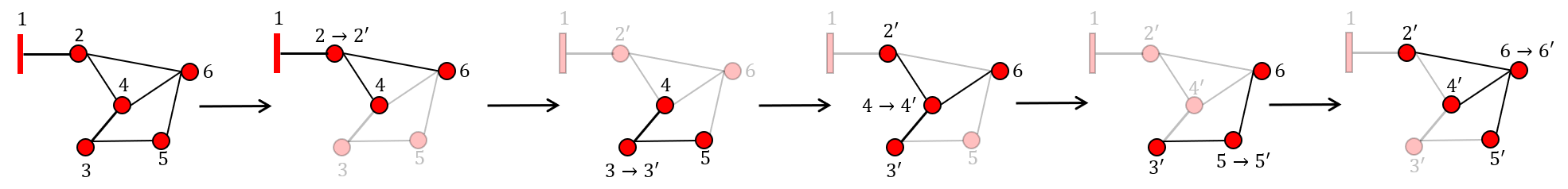
Figure 2: An example of a six bus system where the buses are updated in lexicographical order in one round.

II-B PV Buses

The discussions in the above section focus on PQ buses, but PV buses are also frequently used to describe generators [34]. In this case, the reactive power balance equation in (2) is replaced by a condition on the voltage magnitude:

$$v_{d,r}^{2}+v_{d,i}^{2}=V_{ref}^{2},$$ (6)

where $V_{ref}$ is the reference voltage. Again, we can think of PV buses in term of circles, since (6) is a circle centered at the origin with a fixed radius. Therefore, our framework does not require different treatment of PQ and PV buses.

III Fixed Point Equation for Power Flow

The geometric representation of the power flow equations as the intersection of circles leads to a simple fixed point view of power flow solutions. Suppose that a vector of complex voltages is given. Then, the voltage at a particular bus $d$ is determined by its neighbors as the intersection of the active power circle with the reactive power circle (for a PQ bus) or with the voltage magnitude circle (for a PV bus). Of course, two circles, if they intersect, could do so at two distinct points as shown in Figs. 1(b) and 1(c). In this case, we need to pick one of the intersection points as the complex voltage at a bus and use it to compute the parameter of its neighboring circles. To make this choice, we follow two common assumptions made in power flow calculations.

The first assumption we make is that we are interested in solutions at higher voltage magnitudes [35, 36, 37]. These solutions have long been seen as the practical and stable solutions in actual systems [38]. For example, in both Figs. 1(b) and 1(c), we would chose point $B$ as the solution. For a PV bus, all points of intersection have the same voltage magnitude. In this case, we make the second assumption that voltages with smaller (absolute) angles are preferable. This assumption is rooted in power system stability analysis, where smaller angles indicate more stable stable solutions [39, 40].

With these choices, the complex voltage at a bus is uniquely determined by the complex voltages of its neighbors, which leads to a natural consistency condition for a solution. Given $\mathbf{v}$, let $f$ be a function that takes $\mathbf{v}$ and performs the circle intersection operation (choosing a unique solution as described in the last paragraph). Then a vector $\mathbf{v}$ is a solution to the power flow problem if and only if $\mathbf{v}=f(\mathbf{v})$. That is, $\mathbf{v}$ is a fixed point of $f$. Note that if two circles do not intersect at a bus, then we can declare that $\mathbf{v}$ is not a fixed point.

Here, we use the three bus network in Fig. 1 to illustrate an algorithm to solve the power flow problem. The line admittance of all the branches are $1-j\cdot 1.5$. Bus $1$ is considered to be a slack bus with a voltage of $1$ p.u., while buses $2$ and $3$ are considered to be PQ buses. Initially, the voltage $\mathit{v}_{2}=v_{2,r}+jv_{2,i}$ at bus $2$ is fixed with an initial guess. Based on $\mathit{v}_{2}$, the real and reactive power circles at bus $3$ can be calculated. If these circles intersect with each other, the one with the higher voltage magnitude would be assigned as the value for $v_{3}$. Then, the voltage at bus $3$ is fixed and intersections of the two circles at bus $2$ are used to update $v_{2}$. This is repeated until the convergence is achieved. Tap changing transformers are modeled with fixed tap ratios and incorporated into the admittance matrix using $\pi$ equivalent representations. Next, we describe the algorithm for a general network.

IV Main Algorithm

IV-A Description of the Algorithm

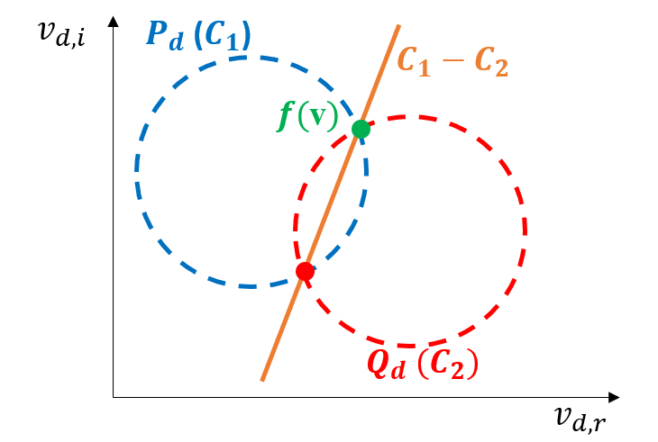
(a) Equation of a line passing through common points of two circles.

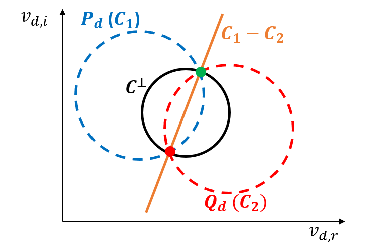
(b) Orthogonal circle passing through common points of two circles.

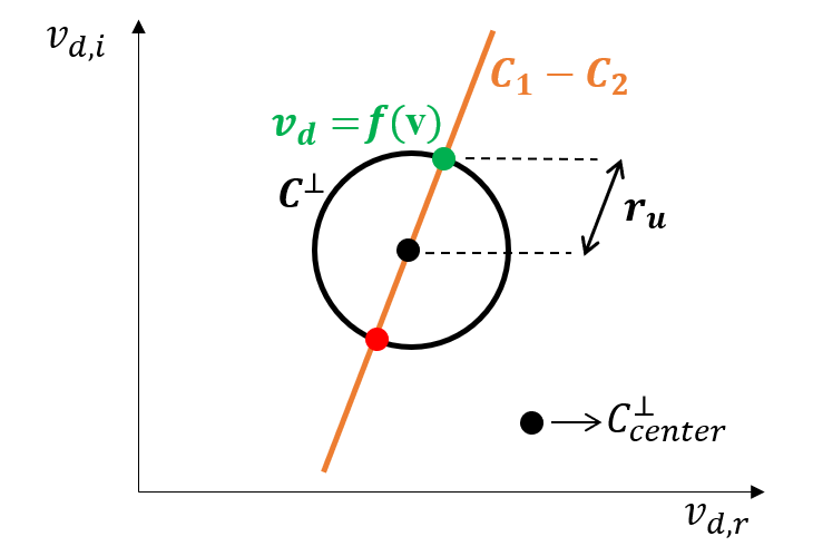
(c) Point of intersection of orthogonal circle and the line passing through common points is $\mathit{v}_{d}=\mathit{f(\mathbf{v})}$.

Figure 3: Geometrical illustration of calculating the voltage solution at a bus.

For an n-bus system, to start the algorithm, the voltages at all the buses in the system are fixed with an initial guess. Then the voltage solution at a bus is updated using its neighbors. This is repeated for all buses, which we call a round of the algorithm. The algorithm terminates if none of the buses update their complex power in a round or when the complex power mismatch is less than the tolerance set by the user. Algorithm 1 presents the pseudo code for a system with only PQ buses. For a system with mixed PQ and PV buses, a similar algorithm can be used, which is given in the Appendix -A.

In our implementation of Algorithm 1, we sweep through all of the buses in one round, as illustrated in Fig. 2 using a lexicographical order. The exact algorithm to find the intersection will be explained in more details in Section IV-B. The exact order of updates is not constrained by the algorithm, although it is an interesting question to see if there exist an “optimal” update order in some sense.

Algorithm 1 Fixed point algorithm for system with only PQ buses.

1:Input  : $\mathit{P}_{i}$, $\mathit{Q}_{i}$ for bus $i=2,\cdots,n$,

2:           Tolerance $\delta$ for the stopping criterion.

3:Output: $\mathit{v}_{i}$ for bus $i=2,\cdots,n$.

4:Initialize voltages at all buses, $\mathit{v}_{i}$ for $i=2,\cdots,n$;

5:Let the neighboring bus index be $k$;

6:where $k$ $\in$ $\mathbb{N}_{m}$. $\triangleright$ $\mathbb{N}_{m}$: Neighboring buses of bus $m$.

7:Calculate the power mismatch ($\Delta\mathbb{S}$);

8:while ($\Delta\mathbb{S})>\delta$ do $\triangleright$ Convergence criteria.

9:        for $m=2$, $\cdots$, $n$ do

10:               Calculate $(\mathit{c}_{p},\mathit{r}_{p})$ at bus $m$, $\forall$ $k$ $\in$ $\mathbb{N}_{m}$;

11:               Calculate $(\mathit{c}_{q},\mathit{r}_{q})$ at bus $m$, $\forall$ $k$ $\in$ $\mathbb{N}_{m}$;

12:               Calculate the voltage $\mathit{v}_{m}$ for bus $m$;

13:               $\mathit{v}_{m}=\mathit{v}_{m}$; $\triangleright$ Update current bus ($m$) voltage.

14:        end for

15:        Calculate ($\Delta\mathbb{S}$);

16:end while

17:return $\mathit{v}_{m}$ $\forall$ buses $m=2,\cdots,n$;

It is possible that the circles do not intersect at a bus either at the start of the algorithm or during one of the iterations. In these cases, we simply restart the algorithm with a new initial guess. We note that for feasible problems with PQ buses, we have never observed the non-intersection of the circles. However for non-feasible problems, it is observed that the algorithm will have non-intersection of circles and further updates in the iterative process are not possible. For mixed PQ and PV systems, it is possible for bad initial guesses to lead to non-intersection behaviors, especially when the loading is very heavy. We will provide more details in Section V.

The proposal algorithm is similar in spirit to the Gauss-Seidel updates used in solving linear equations, where computed results are used as soon as they become available [41]. These type of algorithms are very efficient in memory but can converge slowly. In Section V, we show that our algorithm does not suffer from these potential issues and are competitive with Newton-type methods for large systems.

IV-B Finding Intersection Points

In Algorithm 1, the main computation step is to find the intersection of two circles. At a first glance, this operation is almost trivial and there are many different ways to compute the intersections (see, e.g. [42]). However, the numerical implementation of an intersection algorithm can experience subtle but critical issues. First of all, this operation is called upon many times in the algorithm, and small errors can propagate and result in slower convergence speeds. Second of all, the circles can have very small or large radii. For example, if lines are close to being purely inductive (high $X/R$ ratio), then the reactive circle becomes a circle with a very large radius and straightforward algorithms would run into numerical instabilities. Finally, since finding the intersections takes most of the time in Algorithm 1, it would be desirable to get as close to a closed-form solution as possible. Therefore, we use an unconventional representation of circles developed by [43] to provide a robust and efficient algorithm to find the intersection of circles. For ease of exposition, we focus on system with PQ bus. Analogous results can be derived for PV buses.

Fig. 3 outlines the steps we take to find the intersection of the active and reactive power circles. First, we find the line through the two circles (Fig. 3(a)). Then, we find the smallest circle (called the orthogonal circle) that passes through the intersecting points of the original circles (Fig. 3(b)). Next, we find the intersection of the line with the orthogonal circle (Fig. 3(c)). It turns out that if we view the circles as vectors in a vector space, the above computations can be thought as vector manipulations, which is simple to perform and numerically stable. In the rest of this section, we develop this theory based on the material in [43].

Remark 1.

Note that we do not necessarily require the step in Fig. 3(b). The key reason to compute another circle is that the numerical accuracy of the algorithm improves if the smallest possible circle is used to compute the intersection points as pointed in [43]. Therefore, we use the orthogonal circle, which is the smallest possible circle that contains the intersection points in our algorithm.

IV-C 3-Tuple Vector Representation of Circles

Instead of the traditional center/radius parameterization, we can describe all of the points $\mathbf{x}\in\mathbb{R}^{2}$ on a circle by the following equation:

$$\mathit{a}(\mathit{{\textbf{x}}}\cdot\mathit{{\textbf{x}}})+\mathit{{\textbf{b}}}\cdot\mathit{{\textbf{x}}}+\mathit{c}=0,$$ (7)

where $\cdot$ denotes the dot product between two vectors. The form in (7) allows us to describe a circle using a three tuple $(a,\mathbf{b},c)$. Note that this presentation is not unique, since scaling all of the parameters by a scalar does not change the points that satisfy (7). If $a$ is not zero, we will scale parameters such that $a=1$. In this notation, the circles described by the real and reactive power equations (1) and (2) becomes

$$\left(\mathit{a}_{p},\mathit{{\textbf{b}}}_{p},\mathit{c}_{p}\right)=\left(1,\begin{bmatrix}\frac{t_{d,2}}{t_{d,1}}&\frac{t_{d,3}}{t_{d,1}}\end{bmatrix}^{T},-\frac{\mathit{p}_{d}}{t_{d,1}}\right),$$ (8)

and

$$\left(\mathit{a}_{q},\mathit{{\textbf{b}}}_{q},\mathit{c}_{q}\right)=\left(1,\begin{bmatrix}-\frac{t_{d,3}}{t_{d,4}}&\frac{t_{d,2}}{t_{d,4}}\end{bmatrix}^{T},-\frac{\mathit{q}_{d}}{t_{d,4}}\right).$$ (9)

In these representations, the circles shift gracefully and the same calculations can be applied to a wide range of parameter values even if they approach zero or infinity.

Next, we separate the fixed parameters in the system (e.g., admittance values) and the voltages. Given a bus $d$, let $d_{1},d_{2},\cdots,d_{k}$ its neighboring nodes. Let $\mathbf{g}_{d}=\begin{bmatrix}g_{d_{1},d}&g_{d_{2},d}&\cdots&g_{d_{k},d}\end{bmatrix}$ denote the the vector of conductances between bus $d$ and its neighbors. Similarly, let $\mathbf{b}_{d}=\begin{bmatrix}b_{d_{1},d}&b_{d_{2},d}&\dots&b_{d_{k},d}\end{bmatrix}$ denote the vector of susceptances. Let $\bm{1}$ denote the vector of all $1$’s of the appropriate length. To represent the voltages of the neighboring buses, we use a vector $\mathbf{u}$ formed by concatenating the real and imaginary voltages:

$$\mathbf{u}=\begin{bmatrix}\mathit{v}_{d_{1},r}&\mathit{v}_{d_{2},r}&\cdots&\mathit{v}_{d_{k},r}&\mathit{v}_{d_{1},i}&\mathit{v}_{d_{2},i}&\cdots&\mathit{v}_{d_{k},i}\end{bmatrix}^{T}.$$

Then, we can rewrite (8) and (9) as

$$\left(\mathit{a}_{p},\mathit{{\textbf{b}}}_{p},\mathit{c}_{p}\right)=\left(1,\begin{bmatrix}-\bm{\alpha}&\bm{\delta}\\ -\bm{\delta}&-\bm{\alpha}\end{bmatrix}\mathbf{u},\dfrac{\mathit{p}_{d}}{\bm{1}\cdot\mathbf{g}_{d}}\right),$$ (10)

$$\left(\mathit{a}_{q},\mathit{{\textbf{b}}}_{q},\mathit{c}_{q}\right)=\left(1,\begin{bmatrix}-\bm{\beta}&-\bm{\gamma}\\ \bm{\gamma}&-\bm{\beta}\end{bmatrix}\mathbf{u},\dfrac{\mathit{q}_{d}}{\bm{1}\cdot\mathbf{b}_{d}}\right),$$ (11)

where

$$\alpha=\dfrac{\mathbf{g}_{d}}{\bm{1}\cdot\mathbf{g}_{d}},\beta=\dfrac{\mathbf{b}_{d}}{\bm{1}\cdot\mathbf{b}_{d}},\gamma=\dfrac{\mathbf{g}_{d}}{\bm{1}\cdot\mathbf{b}_{d}},\delta=\dfrac{\mathbf{b}_{d}}{\bm{1}\cdot\mathbf{g}_{d}}.$$

If needed, the centers and radii of power flow circles can be computed easily from (10) and (11):

$$\mathbb{\textbf{Center}}_{p}=\dfrac{-\mathit{\textbf{b}}_{p}}{2},\mathbb{\textbf{Center}}_{q}=\dfrac{-\mathit{\textbf{b}}_{q}}{2},$$ (12)

$$\mathit{r}^{2}_{p}=\left(\dfrac{\mathit{\textbf{b}}_{p}\cdot\mathit{\textbf{b}}_{p}}{4}-\mathit{c}_{p}\right),\mathit{r}^{2}_{q}=\left(\dfrac{\mathit{\textbf{b}}_{q}\cdot\mathit{\textbf{b}}_{q}}{4}-\mathit{c}_{q}\right),$$ (13)

where $\mathbb{\textbf{Center}}_{p}$ and $\mathbb{\textbf{Center}}_{q}$ are the centers of the real and reactive power circles, $r_{p}$ and $r_{q}$ are the radii, respectively.

IV-D Line Passing Through Intersection Points of the Power Flow Circles

Given two circles $C_{1}=(1,\mathit{{\textbf{b}}}_{1},\mathit{c}_{1})$ and $\mathit{C}_{2}=(1,\mathit{{\textbf{b}}}_{2},\mathit{c}_{2})$, the line passing through their points of intersection is described by $C_{1}-C_{2}$, provided the circles intersect. More formally, $C_{1}-C_{2}$ is

$$\mathit{C}_{1}-\mathit{C}_{2}=(0,\mathit{{\textbf{b}}}_{1}-\mathit{{\textbf{b}}}_{2},\mathit{c}_{1}-\mathit{c}_{2})=(0,\mathbf{L}_{2},L_{3})$$ (14)

and describes the points $\mathbf{v}_{d}$ that satisfies the equation

$$\mathit{{\textbf{L}}}_{2}\cdot\mathit{{\textbf{v}}}_{d}+\mathit{L}_{3}=0,$$ (15)

where

$$\mathit{{\textbf{v}}}_{d}=\begin{bmatrix}\mathit{v}_{d,r}\\ \mathit{v}_{d,i}\end{bmatrix}.$$

Substituting (10) and (11) into (15), we have the line described by

$$\left(0,\begin{bmatrix}-\bm{\alpha}+\bm{\beta}&\bm{\gamma}+\bm{\delta}\\ -\left(\bm{\gamma}+\bm{\delta}\right)&-\bm{\alpha}+\bm{\beta}\end{bmatrix}\mathbf{u},\dfrac{\mathit{p}_{d}}{\bm{1}\cdot\mathbf{g}_{d}}+\dfrac{\mathit{q}_{d}}{\bm{1}\cdot\mathbf{b}_{d}}\right).$$ (16)

IV-E Orthogonal Circle

In principle, we can use the line computed in (16) to find the intersection points by intersecting that line with one of the active or reactive circles. However, the numerical accuracy and stability can suffer because the line may intersect the circles at a very acute angle. Therefore, it is more desirable to use the orthogonal circle for calculations. Geometrically, the orthogonal circle is the smallest circle that passes through the two intersection points. Algebraically, we label it as $C^{\perp}$. Again, the parameters of this circle can be computed from (10) and (11) via simple algebra [43, 44]:

$$\mathit{C}^{\perp} =\left(a^{\perp},\mathbf{b}^{\perp},c^{\perp}\right)$$

$$=\left(1,\dfrac{\mathit{{\textbf{b}}}_{1}+\mathit{{\textbf{b}}}_{2}}{2}+\dfrac{\left(\mathit{{\textbf{b}}}_{2}-\mathit{{\textbf{b}}}_{1}\right)\left(\mathit{k}^{2}_{1}-\mathit{k}^{2}_{2}\right)}{2\left\|\mathit{{\textbf{b}}}_{1}-\mathit{{\textbf{b}}}_{2}\right\|^{2}},\right.$$

$$\left.~{}~{}~{}~{}\dfrac{\mathit{c}_{1}+\mathit{c}_{2}}{2}+\dfrac{\left(\mathit{c}_{2}-\mathit{c}_{1}\right)\left(\mathit{k}^{2}_{1}-\mathit{k}^{2}_{2}\right)}{2\left\|\mathit{{\textbf{b}}}_{1}-\mathit{{\textbf{b}}}_{2}\right\|^{2}}\right),$$ (17)

where

$$\mathit{k}^{2}_{1} =\|\mathit{{\textbf{b}}}_{1}\|^{2}-4\mathit{a}_{1}\mathit{c}_{1},$$

$$\mathit{k}^{2}_{2} =\|\mathit{{\textbf{b}}}_{2}\|^{2}-4\mathit{a}_{2}\mathit{c}_{2}.$$

Here, $\|~{}\|$ is the standard $l_{2}$ norm. The center and the radius of the orthogonal circle is given by

$$\mathit{\textbf{Center}}^{\perp}=\dfrac{-\mathbf{b}^{\perp}}{2}$$ (18)

and

$$\mathit{r}_{u}=\sqrt{\dfrac{\mathbf{b}^{\perp}\cdot\mathbf{b}^{\perp}}{4}-c^{\perp}}.$$ (19)

Substituting (10) and (11) in (17), we get

$$\mathit{C}^{\perp} =\left(1,\frac{1}{2}\mathbf{M}_{B}\mathbf{u}+\dfrac{\left(\dfrac{\left\|\mathbf{u}\right\|^{2}}{2}\cdot\mathit{K}_{c}-2\cdot l\right)\mathbf{M}_{A}\mathbf{u}}{\left\|\mathbf{M}_{A}\mathbf{u}\right\|^{2}},\right.$$

$$\left.\dfrac{1}{2}\left(\dfrac{\mathit{p}_{d}}{\bm{1}\cdot\mathbf{g}_{d}}-\dfrac{\mathit{q}_{d}}{\bm{1}\cdot\mathbf{b}_{d}}\right)+\dfrac{l\left(2l-\dfrac{\left\|\mathbf{u}\right\|^{2}}{2}\mathit{K}_{c}\right)}{\left\|\mathbf{M}_{A}\mathbf{u}\right\|^{2}}\right),$$ (20)

where

$$\mathbf{M}_{A} =\begin{bmatrix}\bm{\alpha}-\bm{\beta}&-\left(\bm{\gamma}+\bm{\delta}\right)\\ \bm{\gamma}+\bm{\delta}&\bm{\alpha}-\bm{\beta}\end{bmatrix}\mathbf{M}_{B}=\begin{bmatrix}-\left(\bm{\alpha}+\bm{\beta}\right)&\bm{\delta}-\bm{\gamma}\\ -\left(\bm{\delta}-\bm{\gamma}\right)&-\left(\bm{\alpha}+\bm{\beta}\right)\end{bmatrix},$$

$$l =\dfrac{\mathit{p}_{d}}{\bm{1}\cdot\mathbf{g}_{d}}+\dfrac{\mathit{q}_{d}}{\bm{1}\cdot\mathbf{b}_{d}},~{}\mathit{K}_{c}=\left(\|\bm{\alpha}\|^{2}+\|\bm{\delta}\|^{2}\right)-\left(\|\bm{\gamma}\|^{2}+\|\bm{\beta}\|^{2}\right).$$

IV-F Point of Intersection

Next, we find the point of intersection (Fig. 3(c)). These points are found at a distance of $\mathit{r}_{u}$ from the center of orthogonal circle along the line computed in (16). Through simple algebra, we compute the point of intersection, that is, the updated voltage at bus $d$ given by

$$\begin{bmatrix}v_{d,r}\\ v_{d,i}\end{bmatrix} =\mathit{\textbf{Center}}^{\perp}\pm\mathit{r}_{u}\dfrac{\mathbf{R}\mathit{{\textbf{L}}}_{2}}{\left\|\mathit{{\textbf{L}}}_{2}\right\|^{2}}$$

$$=-\frac{\mathbf{b}^{\perp}}{2}\pm\sqrt{\dfrac{\mathbf{b}^{\perp}\cdot\mathbf{b}^{\perp}}{4}-c^{\perp}}\cdot\dfrac{\mathbf{R}\mathit{{\textbf{L}}}_{2}}{\left\|\mathit{{\textbf{L}}}_{2}\right\|^{2}},$$ (21)

$$=\frac{-1}{4}\mathbf{M}_{B}\mathbf{u}-\dfrac{\left(\dfrac{\left\|\mathbf{u}\right\|^{2}}{2}\cdot\mathit{K}_{c}-2\cdot l\right)\mathbf{M}_{A}\mathbf{u}}{2\cdot\left\|\mathbf{M}_{A}\mathbf{u}\right\|^{2}}\pm$$

$$\left(\dfrac{1}{4}\cdot\left\|\frac{1}{2}\mathbf{M}_{B}\mathbf{u}+\dfrac{\left(\dfrac{\left\|\mathbf{u}\right\|^{2}}{2}\cdot\mathit{K}_{c}-2\cdot l\right)\mathbf{M}_{A}\mathbf{u}}{\left\|\mathbf{M}_{A}\mathbf{u}\right\|^{2}}\right\|^{2}-\right.$$

$$\left.\dfrac{1}{2}\left(\dfrac{\mathit{p}_{d}}{\bm{1}\cdot\mathbf{g}_{d}}-\dfrac{\mathit{q}_{d}}{\bm{1}\cdot\mathbf{b}_{d}}\right)+\dfrac{l\left(2l-\dfrac{\left\|\mathbf{u}\right\|^{2}}{2}\mathit{K}_{c}\right)}{\left\|\mathbf{M}_{A}\mathbf{u}\right\|^{2}}\right)^{\dfrac{1}{2}}\cdot\dfrac{\mathbf{R}\mathit{{\textbf{L}}}_{2}}{\left\|\mathit{{\textbf{L}}}_{2}\right\|^{2}}.$$

where

$$\mathbf{R}=\begin{bmatrix}0&-1\\ 1&0\end{bmatrix}$$

and $\mathbf{b}^{\perp}$ is given by (17) and $\mathbf{L}_{2}$ is given by (14). To choose one solution or a sign in (21), we will pick the one that leads to the higher voltage magnitude. Note that in (21), most of the computation can be done offline since they only involve the admittance parameters. Applying (21) to every bus $d$ also gives us an analytical form of the fixed point equation for the complex voltages.

V Numerical Results

In this section, simulation studies on standard IEEE test cases, specifically with the 4, 14, 30, 39, 57, 118, 2383 and 3375 bus systems. Their information are obtained from the Matpower software [45]. The proposed fixed point algorithm are compared with other power flow methods at nominal loading and heavy loading conditions. We also test the sensitivity of these algorithm to the initializaton points. In particular, we will consider five algorithms: 1) FP, our proposed algorithm; 2) GS, the standard Gauss-Seidel algorithm; 3) NR, the standard Newton-Raphson algorithm; 4) FDLF, the fast decoupled load flow algorithm and 5) Iwamoto, a Jacobian-based adjustable step size method (sometimes called non-divergent power flow method) [23].

V-A Performance of Proposed Method

First we study the convergence of the proposed FP algorithm on the standard $14$-, $30$- and $118$-IEEE bus systems are shown in Fig. 4 under nominal loading conditions. More precisely, we take the data from MatPower [45] and run our fixed point algorithm to test its convergence. As shown in Fig. 4, for these standard cases, the fixed point algorithm converges in tens of iterations. Since each iteration is cheap to compute, the convergence time is in 10s of milliseconds.

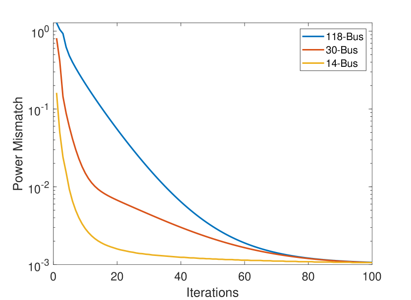
Figure 4: Semi-log plot of the convergence of the fixed point algorithm for IEEE standard systems at base case loading.

Next, we compare the convergence speed of FP with NR and Iwamoto algorithms for a variety of systems. In addition to using the nominal loading, we introduce a scaling parameter $\lambda$ to scale the loads and generations by multiplying both the active and reactive powers by $\lambda$. The performance of all three algorithms are shown in Fig. 5 in a log-scale. As expected, when the networks are small, NR and Iwamoto methods converges very quickly since they only require a few (sometimes only 1) updates. As the test cases becomes bigger, the FP method start to catch up. For the largest two test systems (2383-bus and 3375-bus), FP is comparable with Iwamoto and faster than NR. In addition, convergence times for FP is much less sensitive to the system size, which is expected since there are not matrix computations.

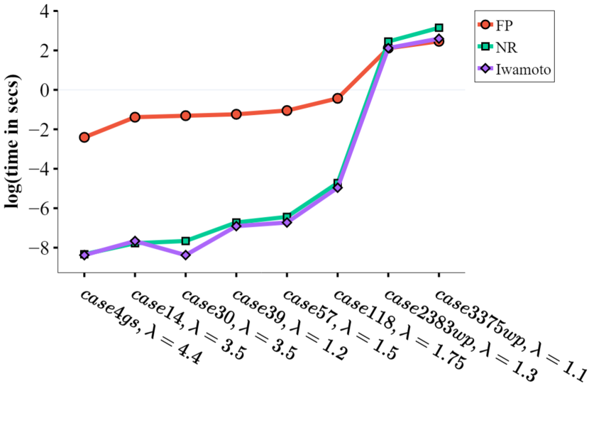
Figure 5: Time taken to attain the desired precision by FP, NR and Iwamoto’s method for different size systems under different load scaling parameters $\lambda$. As the systems become large, FP becomes competitive with the other two methods.

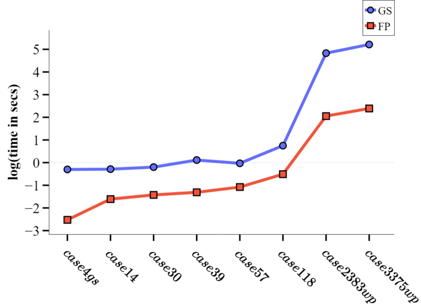
Figure 6: Time taken to attain the desired precision by GS and FP method for different size systems at base case loading. FP is faster than GS for all of the IEEE systems.

Fig. 6 compares the convergence speed of FP and GS for a variety of systems. GS calculates the voltage solutions at every bus in the system via a lexicographical approach. Even though GS is partly similar to the proposed approach, the fixed point equation used to calculate the voltages in both the methods are different. This difference makes the FP perform faster when compared to GS as shown in Fig. 6.

V-B Heavily Loaded Networks

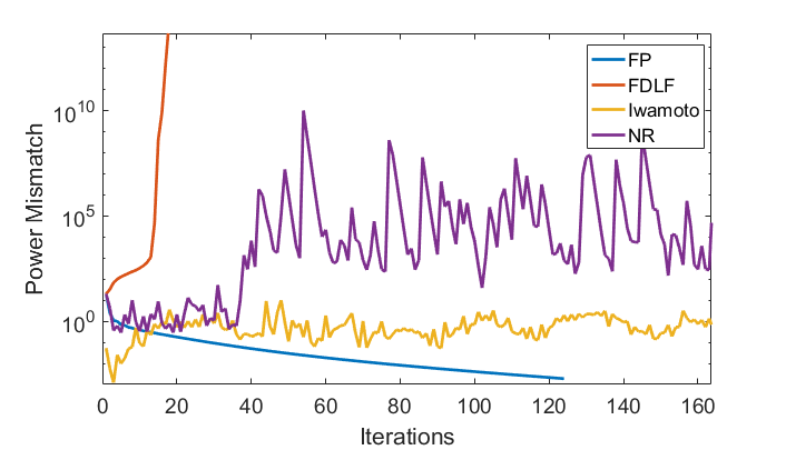
Figure 7: Convergence performance of FP compared with NR, Iwamoto and FDLF. The test system is the IEEE 14-bus system with loads scaled by a factor of 3.99. At this loading, the FP method converges reliably to the solution while the other methods either diverges or exhibit oscillatory behavior.

The more challenging setting, and the setting the FP algorithm is designed to address, is when the systems are heavily loaded. For example, we take the $14$-bus network and increase all of the loads by a factor of 3.99. This loading is still feasible, but is very close to the loadability limit of the system. Figure 7 presents the convergence comparison of the methods. As expected, NR diverges [46, 47] since the Jocabian matrix is very ill-conditioned around the solution. The FDLF also diverges, while it does not face conditioning problems since the Jacobian is approximated by a fixed matrix in decoupled load flow, the update direction provided by the fixed Jacobian becomes invalid and the algorithm diverges very quickly. Interestingly, the optimal multiplier method (Iwamoto [23]) also becomes unstable because of numerical issues. More precisely, the multiplier $\mu$ is used to control the step size in the following update:

$$\Delta\mathit{V}=\mu\cdot\left(J^{-1}\right)\cdot\left(\Delta\mathit{S}\right).$$ (22)

However, if $J$ is very ill-conditioned, then we are essentially multiplying a very small number by a very large number, which creates problems due to finite machine precision.

Similar behaviors to Fig. 7 are observed in IEEE $4$-, $30$- and $118$-bus systems for load multiplier of 4.5, 3.65 and 1.78, respectively. In contrast, our proposed method is able to converge even under these conditions since it does not use the power flow Jacobian. This illustrates the envisioned utility of the proposed FP method in practice. An operator can use conventional power flow solvers and when they do not converge, instead of fine tuning parameters or trying many different initialization points, the FP algorithm can be used as a viable tool to obtain convergence.

Figure 8 compares the performance of the FP, NR, FDLF and Iwamoto algorithms in more detail. As we can see, the NR algorithm jumps erratically in the voltage space. The Iwamoto method controls this behavior by scaling the updates by $\mu$, but even though it prevents the algorithm from diverging, it cannot converge reliably and instead oscillate around the solution. The FP algorithm again converges reliably and do not oscillate. It does not encounter the numerical instabilities of other methods since the only calculation required is the intersection of two circles (regardless of the system size), and these intersections can be handled gracefully even when the circles becomes degenerate using the algorithm in Section IV-B.

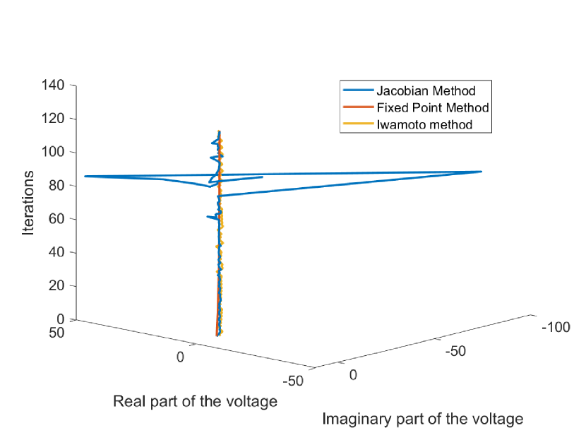
(a) Updates of the real and imaginary parts of the voltage vector

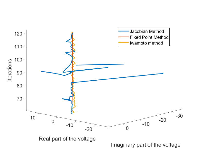
(b) Zoomed in view of Fig. 8(a) showing the oscillatory behavior of the Iwamoto method.

Figure 8: Comparison of NR, FP and Iwamoto’s voltage updates at bus $4$ in IEEE-$14$ bus system under the loading condition of Fig. 7.

V-C Sensitivity to Initial Conditions

In addition to convergence, it is important for an algorithm to be robust to the initial conditions, especially as the randomness in the system increases due to renewable integration [18]. To test the performance of various algorithms to initial conditions, we take the IEEE 30-bus system at its standard loading and randomly select the starting voltages. In our experiments, we set the initial guess to be random samples from the uniform distribution on the interval $\left[1-\alpha,1+\alpha\right]$ for various values of $\alpha$ (we always set the imaginary part to be 0) , independently for each bus. Table I reports the number of successful convergences (defined as power mismatch convergence less than $0.001$ p.u.) for the FDLF, NR, optimal multiplier and our proposed FP methods for 100 trials.

Initialization spread $\alpha$	NR	FDLF	optimal multiplier	FP
0.05	100	98	100	100
0.1	64	62	100	100
0.2	4	0	0	100
0.3	0	0	0	100
0.4	0	0	0	100
0.6	0	0	0	100
0.9	0	0	0	100

TABLE I: Convergence test of the power flow methods with random initialization for 100 trials. The initial voltages are generated identical and independently from uniform distribution of $[1-\alpha,1+\alpha]$. Our proposed method converged for every trial, where as other methods quickly stopped working once the range become moderately large.

As we see in Table I, our proposed FP method is much more robust to the value of the initial guesses than the other methods: it always converged while the other methods quickly stopped working when $\alpha$ becomes large. Hence it is observed that the phenomenon of power flow fractals is not exhibited by the proposed method unlike NR based methods [48, 49]. This hints that the fixed point method may avoid being trapped in local optima that can impact descent algorithms since local optima are not fixed points by definition.

VI Conclusion

A new fixed-point formulation of the power flow equation is developed in this paper. In contrast to existing fixed point formulations, it includes all possible cases of PV/PQ buses, mesh networks, resistive and inductive lines. Geometrically, our formulation treats the active and reactive power flow equations in rectangular voltage coordinates as circles and the power flow solutions as the intersection of these circles. Using a 3-tuple vector representation of circles, we derive simple, efficient and numerically stable formulas to find their intersection points. Based on the fixed point equations, we develop a natural iterative fixed point algorithm to solve the power flow problem. Numerical studies on the standard IEEE benchmarks show that our algorithm is able to converge when other state-of-the-art algorithms diverges or becomes unstable. We also show that the performance of proposed algorithm is comparable to other Jacobian based methods for large test systems. In addition, we show that our algorithm is robust to the initial starting point, able to converge for a wide range of starting conditions while other algorithms diverged.

-A Handling PQ and PV buses

Here we present the fixed-point algorithm for a system with both PQ and PV buses. In the case of PV buses, Section II-B discusses the replacement of the reactive power balance equation by a condition on the voltage magnitude (6). The voltage circle is centered at origin ($\mathit{c}_{v}$) with fixed radius of $\mathit{V}_{ref}$ ($\mathit{r}_{v}$). Thus the voltage solution for a PV bus can be calculated similarly to PQ bus by the intersection of two circles, real power (1) and specified voltage magnitude circles (6) at bus $d$.

-B Bus Type Switching for PV Buses

-B1 PV to PQ switching

When there are no common points between the real power and specified voltage magnitude circles, the reactive power at bus $d$ is calculated to check for the violation of reactive power limits. In such a scenario, the PV bus is converted to a PQ bus by fixing its reactive power with the violated limit and it is then solved as a PQ bus. During the iterative process, this PQ bus is converted back to a PV bus as discussed below.

-B2 PQ to PV switching

The bus that is converted to PQ has its real and reactive power fixed while the voltage phase angle and magnitude are free to change. However, this bus should be reverted to PV bus during the power flow iterative process when it is feasible since the problem still didn’t converge. Let the voltage solution at this converted PQ bus be $v$. The violated upper and lower limit reactive powers be represented by $Q_{max}$ and $Q_{min}$ respectively. A converted PQ bus (due to PV to PQ switching) with $Q=Q_{max}$ or $Q=Q_{min}$ is referred as $PQ_{max}$ bus or $PQ_{min}$ bus respectively. For $PQ_{max}$ bus, when $v>\mathit{V}_{ref}$ it indicates that the reactive power at this bus is no longer needed to be fixed at $Q_{max}$ and it can be reverted back to a PV bus. Similarly for $PQ_{min}$ bus as well but the conditions to check is reversed to $v<\mathit{V}_{ref}$.

Algorithm 2 RFPPF method for PQ and PV buses.

1:Input  : $\mathit{P}_{i}$ for bus $i=2,\cdots,n$,

2:           $\mathit{Q}_{i}$ $\forall$ PQ buses,

3:           $\mathit{V}_{ref}$ $\forall$ PV buses,

4:           $\mathit{Q}_{max}$ and $\mathit{Q}_{min}$ for PV buses,

5:             Bus type information $B\{i\}$ for bus $i=2,\cdots,n$,

6:           Tolerance $\delta$ for the stopping criterion.

7:Output: $\mathit{v}_{i}$ for bus $i=2,\cdots,n$.

8:Initialize voltages at all buses, $\mathit{v}_{i}$ for $i=2,\cdots,n$;

9:Let the neighboring bus index be $k$;

10:where $k$ $\in$ $\mathbb{N}_{m}$. $\triangleright$ $\mathbb{N}_{m}$: Neighboring buses of bus $m$.

11:Calculate the power mismatch ($\Delta\mathbb{S}$);

12:while ($\Delta\mathbb{S})>\delta$ do $\triangleright$ Convergence criteria.

13:        for $m=2$, $\cdots$, $n$ do

14:               if $B\{m\}$ == PQ bus then

15:                       Calculate $(\mathit{c}_{p},\mathit{r}_{p})$ at bus $m$, $\forall$ $k$ $\in$ $\mathbb{N}_{m}$;

16:                       Calculate $(\mathit{c}_{q},\mathit{r}_{q})$ at bus $m$, $\forall$ $k$ $\in$ $\mathbb{N}_{m}$;

17:                       Calculate the voltage $\mathit{v}_{m}$ for bus $m$;

18:                       $\mathit{v}_{m}=\mathit{v}_{m}$; $\triangleright$ Update bus $m$ voltage.

19:                       if $B\{m\}==PQ_{max}$ and $\mathit{v}_{m}>\mathit{V}_{ref}$ then

20:                              Revert to PV bus and update $B\{m\}$;

21:                       end if

22:                       if $B\{m\}==PQ_{min}$ and $\mathit{v}_{m}<\mathit{V}_{ref}$ then

23:                              Revert to PV bus and update $B\{m\}$;

24:                       end if

25:               else$\triangleright$ PV bus.

26:                       Calculate $(\mathit{c}_{p},\mathit{r}_{p})$ at bus $m$, $\forall$ $k$ $\in$ $\mathbb{N}_{m}$;

27:                       Calculate $(\mathit{c}_{v},\mathit{r}_{v})$ at bus $m$, $\forall$ $k$ $\in$ $\mathbb{N}_{m}$;

28:                       if Circles $(\mathit{c}_{p},\mathit{r}_{p})$ and $(\mathit{c}_{v},\mathit{r}_{v})$ intersect then

29:                              Calculate the voltage $\mathit{v}_{m}$ for bus $m$;

30:                              $\measuredangle\mathit{v}_{m}=\measuredangle\mathit{v}_{m}$; $\triangleright$ Update voltage angle.

31:                       else

32:                              Convert bus $m$ to PQ bus & update $B\{m\}$;

33:                              Calculate $(\mathit{c}_{p},\mathit{r}_{p})$ at bus $m$;

34:                              Calculate $(\mathit{c}_{q},\mathit{r}_{q})$ at bus $m$;

35:                              Calculate the voltage $\mathit{v}_{m}$ for bus $m$;

36:                              $\mathit{v}_{m}=\mathit{v}_{m}$; $\triangleright$ Update bus $m$ voltage.

37:                       end if

38:               end if

39:        end for

40:        Calculate ($\Delta\mathbb{S}$);

41:end while

42:return $\mathit{v}_{m}$ $\forall$ buses $m=2,\cdots,n$;

Kishan Prudhvi Guddanti received the B.Tech. degree in electrical engineering from Sri Ramaswamy Memorial Institute of Science and Technology, Chennai, India and the M.Sc degree in electrical engineering from Arizona State University, Tempe, AZ, USA. He is currently pursuing the Ph.D. degree at Arizona State University, Tempe, AZ, USA. He is one of the winners of an AI competition organized by RTE France in 2019. His current research interest is in the interdisciplinary area of AI applications in power systems in addition to voltage stability and data-driven techniques applications in power system risk assessment and control.

Yang Weng received the B.E. degree in electrical engineering from Huazhong University of Science and Technology, Wuhan, China; the M.Sc. degree in statistics from the University of Illinois at Chicago, Chicago, IL, USA; and the M.Sc. degree in machine learning of computer science and M.E. and Ph.D. degrees in electrical and computer engineering from Carnegie Mellon University (CMU), Pittsburgh, PA, USA. After finishing his Ph.D., he joined Stanford University, Stanford, CA, USA, as the TomKat Fellow for Sustainable Energy. He is currently an Assistant Professor of electrical, computer and energy engineering at Arizona State University (ASU), Tempe, AZ, USA. His research interest is in the interdisciplinary area of power systems, machine learning, and renewable integration. Dr. Weng received the CMU Dean’s Graduate Fellowship in 2010, the Best Paper Award at the International Conference on Smart Grid Communication (SGC) in 2012, the first ranking paper of SGC in 2013, Best Papers at the Power and Energy Society General Meeting in 2014, ABB fellowship in 2014, Golden Best Paper Award at the International Conference on Probabilistic Methods Applied to Power Systems in 2016, and Best Paper Award at IEEE Conference on Energy Internet and Energy system Integration in 2017

Baosen Zhang received his Bachelor of Applied Science in Engineering Science degree from the University of Toronto in 2008; and his PhD degree in Electrical Engineering and Computer Sciences from University of California, Berkeley in 2013. He was a Postdoctoral Scholar at Stanford University, affiliated with the Civil and Environmental Engineering and Management & Science Engineering. He is currently the Keith and Nancy Rattie Endowed Career Development Professor in the Departement of Electrical and Computer Engineering at the University of Washington, Seattle, WA. His research interests are in power systems and cyberphysical systems.

References

- [1] B. Stott, “Review of load-flow calculation methods,” Proceedings of the IEEE, vol. 62, no. 7, pp. 916–929, 1974.
- [2] J. D. Glover, M. S. Sarma, and T. Overbye, Power System Analysis & Design, SI Version. Cengage Learning, 2012.
- [3] J. A. Momoh, M. E. El-Hawary, and R. Adapa, “A review of selected optimal power flow literature to 1993. ii. newton, linear programming and interior point methods,” IEEE Transactions on Power Systems, vol. 14, no. 1, pp. 105–111, Feb 1999.
- [4] B. Stott and O. Alsac, “Fast decoupled load flow,” IEEE transactions on power apparatus and systems, no. 3, pp. 859–869, 1974.
- [5] A. Monticelli, A. Garcia, and O. R. Saavedra, “Fast decoupled load flow: Hypothesis, derivations, and testing,” IEEE Transactions on Power systems, vol. 5, no. 4, pp. 1425–1431, 1990.
- [6] J. Thorp and S. Naqavi, “Load flow fractals,” in Decision and Control, 1989., Proceedings of the 28th IEEE Conference on. IEEE, 1989, pp. 1822–1827.
- [7] J. S. Thorp, S. A. Naqavi, and H. . Chiang, “More load flow fractals,” in 29th IEEE Conference on Decision and Control, Dec 1990, pp. 3028–3030 vol.6.
- [8] S. Rao and D. Tylavsky, “Theoretical convergence guarantees versus numerical convergence behavior of the holomorphically embedded power flow method,” International Journal of Electrical Power and Energy Systems, vol. 95, pp. 166–176, 2 2018.
- [9] D. Pudjianto, C. Ramsay, and G. Strbac, “Virtual power plant and system integration of distributed energy resources,” IET Renewable Power Generation, vol. 1, no. 1, pp. 10–16, 2007.
- [10] B. Zhang and D. Tse, “Geometry of injection regions of power networks,” IEEE Transactions on Power Systems, vol. 28, no. 2, pp. 788–797, 2013.
- [11] I. A. Hiskens and R. J. Davy, “Exploring the power flow solution space boundary,” IEEE Transactions on Power Systems, vol. 16, no. 3, pp. 389–395, Aug 2001.
- [12] V. Ajjarapu and C. Christy, “The continuation power flow: a tool for steady state voltage stability analysis,” IEEE transactions on Power Systems, vol. 7, no. 1, pp. 416–423, 1992.
- [13] B. Stott, “Effective starting process for newton-raphson load flows,” in Proceedings of the institution of electrical engineers, vol. 118, no. 8. IET, 1971, pp. 983–987.
- [14] S. Iwamoto and Y. Tamura, “A fast load flow method retaining nonlinearity,” The transactions of the Institute of Electrical Engineers of Japan. B, vol. 98, no. 2, pp. 192–198, 1978.
- [15] C. A. Canizares and F. L. Alvarado, “Point of collapse and continuation methods for large ac/dc systems,” IEEE transactions on Power Systems, vol. 8, no. 1, pp. 1–8, 1993.
- [16] H.-D. Chiang, T.-Q. Zhao, J.-J. Deng, and K. Koyanagi, “Homotopy-enhanced power flow methods for general distribution networks with distributed generators,” IEEE Trans. Power Syst, vol. 29, no. 1, pp. 93–100, 2014.
- [17] F. Milano, “Continuous newton’s method for power flow analysis,” IEEE Transactions on Power Systems, vol. 24, no. 1, pp. 50–57, 2009.
- [18] V. Da Costa and A. Rosa, “A comparative analysis of different power flow methodologies,” in Transmission and Distribution Conference and Exposition: Latin America, 2008 IEEE/PES. IEEE, 2008, pp. 1–7.
- [19] A. Gómez-Expósito and C. Gómez-Quiles, “Factorized load flow,” IEEE Transactions on Power Systems, vol. 28, no. 4, pp. 4607–4614, 2013.
- [20] W. F. Tinney and C. E. Hart, “Power flow solution by newton’s method,” IEEE Transactions on Power Apparatus and systems, no. 11, pp. 1449–1460, 1967.
- [21] A. Shahriari, H. Mokhlis, and A. Bakar, “Critical reviews of load flow methods for well, ill and unsolvable condition,” Journal of Electrical Engineering, vol. 63, no. 3, pp. 144–152, 2012.
- [22] A. J. Wood and B. F. Wollenberg, Power generation, operation, and control. John Wiley & Sons, 2012.
- [23] S. Iwamoto and Y. Tamura, “A load flow calculation method for ill-conditioned power systems,” IEEE transactions on power apparatus and systems, no. 4, pp. 1736–1743, 1981.
- [24] C. Castro and L. Braz, “A new approach to the polar newton power flow using step size optimization,” in Proceedings of the 29th North American Symposium, Laramie, Wyoming, USA, 1997.
- [25] L. M. Braz, C. A. Castro, and C. Murati, “A critical evaluation of step size optimization based load flow methods,” IEEE Transactions on Power Systems, vol. 15, no. 1, pp. 202–207, 2000.
- [26] P. R. Bijwe and S. M. Kelapure, “Nondivergent fast power flow methods,” IEEE Transactions on Power Systems, vol. 18, no. 2, pp. 633–638, May 2003.
- [27] M. Pirnia, C. A. Cañizares, and K. Bhattacharya, “Revisiting the power flow problem based on a mixed complementarity formulation approach,” IET Generation, Transmission Distribution, vol. 7, no. 11, pp. 1194–1201, November 2013.
- [28] Y.-H. Moon, H.-J. Koo, J.-G. Lee, Y.-J. Kwon, and B.-M. Yang, “Energy-based power system analysis with the equivalent mechanical model,” IFAC Proceedings Volumes, vol. 36, no. 20, pp. 599–604, 2003.
- [29] J. W. Simpson-Porco, “A theory of solvability for lossless power flow equations–part i: Fixed-point power flow,” IEEE Transactions on Control of Network Systems, 2017.
- [30] C. Wang, A. Bernstein, J.-Y. Le Boudec, and M. Paolone, “Explicit conditions on existence and uniqueness of load-flow solutions in distribution networks,” IEEE Transactions on Smart Grid, 2016.
- [31] S. Kakutani et al., “A generalization of brouwer’s fixed point theorem,” Duke mathematical journal, vol. 8, no. 3, pp. 457–459, 1941.
- [32] G. L. Torres and V. H. Quintana, “An interior-point method for nonlinear optimal power flow using voltage rectangular coordinates,” IEEE transactions on Power Systems, vol. 13, no. 4, pp. 1211–1218, 1998.
- [33] Y. Weng, R. Rajagopal, and B. Zhang, “Geometric understanding of the stability of power flow solutions,” arXiv preprint arXiv:1706.07401, 2017.
- [34] P. A. Garcia, J. L. R. Pereira, S. Carneiro, V. M. da Costa, and N. Martins, “Three-phase power flow calculations using the current injection method,” IEEE Transactions on Power Systems, vol. 15, no. 2, pp. 508–514, 2000.
- [35] I. Dobson and H.-D. Chiang, “Towards a theory of voltage collapse in electric power systems,” Systems & Control Letters, vol. 13, no. 3, pp. 253 – 262, 1989. [Online]. Available: http://www.sciencedirect.com/science/article/pii/0167691189900728
- [36] H. G. Kwatny, R. F. Fischl, and C. O. Nwankpa, “Local bifurcation in power systems: theory, computation, and application,” Proceedings of the IEEE, vol. 83, no. 11, pp. 1456–1483, 1995.
- [37] B. K. Johnson, “Extraneous and false load flow solutions,” IEEE Transactions on Power Apparatus and Systems, vol. 96, no. 2, pp. 524–534, March 1977.
- [38] D. Mehta, D. K. Molzahn, and K. Turitsyn, “Recent advances in computational methods for the power flow equations,” in American Control Conference (ACC), 2016. IEEE, 2016, pp. 1753–1765.
- [39] P. Kundur, N. J. Balu, and M. G. Lauby, Power system stability and control. McGraw-hill New York, 1994, vol. 7.
- [40] C. Vournas, P. Sauer, and M. Pai, “Relationships between voltage and angle stability of power systems,” International Journal of Electrical Power & Energy Systems, vol. 18, no. 8, pp. 493–500, 1996.
- [41] L. A. Hageman and D. M. Young, Applied iterative methods. Courier Corporation, 2012.
- [42] E. Weisstein, “Circle-circle intersection,” Wolfram Research, Inc., 2003. [Online]. Available: http://mathworld.wolfram.com/Circle-CircleIntersection.html
- [43] A. E. Middleditch, T. Stacey, and S. B. Tor, “Intersection algorithms for lines and circles,” ACM Transactions on Graphics (TOG), vol. 8, no. 1, pp. 25–40, 1988.
- [44] H. G. Baker, “Corrigenda: intersection algorithms for lines and circles,” ACM Transactions on Graphics (TOG), vol. 13, no. 3, pp. 308–310, 1994.
- [45] R. D. Zimmerman, C. E. Murillo-Sánchez, R. J. Thomas et al., “Matpower: Steady-state operations, planning, and analysis tools for power systems research and education,” IEEE Transactions on power systems, vol. 26, no. 1, pp. 12–19, 2011.
- [46] T. Van Cutsem and C. Vournas, Voltage stability of electric power systems. Springer Science & Business Media, 2007.
- [47] T. Van Cutsem, “Voltage instability: phenomena, countermeasures, and analysis methods,” Proceedings of the IEEE, vol. 88, no. 2, pp. 208–227, 2000.
- [48] J. S. Thorp and S. A. Naqavi, “Load-flow fractals draw clues to erratic behaviour,” IEEE Computer Applications in Power, vol. 10, no. 1, pp. 59–62, 1997.
- [49] R. P. Klump and T. Overbye, “A new method for finding low-voltage power flow solutions,” in 2000 Power Engineering Society Summer Meeting (Cat. No. 00CH37134), vol. 1. IEEE, 2000, pp. 593–597.