Existence and stability of dust ion acoustic double layers described by the combined MKP-KP equation

Abstract

The purpose of this paper is to expand the recent work of Sardar et al. [Phys. Plasmas 23, 123706 (2016)] on the existence and stability of alternative dust ion acoustic solitary wave solution of the combined modified Kadomtsev Petviashvili - Kadomtsev Petviashvili (MKP-KP) equation in a nonthermal plasma. Sardar et al. [Phys. Plasmas 23, 123706 (2016)] have derived a combined MKP-KP equation to describe the nonlinear behaviour of the dust ion acoustic wave when the coefficient of the nonlinear term of the KP equation tends to zero. Sardar et al. [Phys. Plasmas 23, 123706 (2016)] have used this combined MKP-KP equation to investigate the existence and stability of the alternative solitary wave solution having a profile different from $\mbox{sech}^{2}$ or sech when $L>0$, where $L$ is a function of the parameters of the present plasma system. In the present paper, we have considered the same combined MKP-KP equation to study the existence and stability of the double layer solution and it is shown that double layer solution of this combined MKP-KP equation exists if $L=0$. Finally, the lowest order stability of the double layer solution of this combined MKP-KP equation has been investigated with the help of multiple scale perturbation expansion method of Allen and Rowlands [ J. Plasma Phys. 50, 413 (1993)]. It is found that the double layer solution of the combined MKP-KP equation is stable at the lowest order of the wave number for long-wavelength plane-wave perturbation.

I Introduction

In last few decades, much emphasis has been given to understand the nonlinear wave processes in dusty plasmas. Formation of double layers (DLs) in a multispecies unmagnetized or magnetized plasma is an interesting nonlinear phenomena in many areas of space plasma physics Block (1972); Mozer et al. (1977); Sato and Okuda (1980); Hudson and Potter (1981); Temerin et al. (1982); Schamel (1986); Kim (1987); Schamel (1987); Boström et al. (1988); Boström (1992); Han and Kim (1994); Dovner et al. (1994); Mozer and Kletzing (1998); Ergun et al. (2002); Main, Newman, and Ergun (2006); Kim et al. (2007); Angelopoulos (2008); Ergun et al. (2009); Li et al. (2015) as well as in various types of laboratory plasmas Coakley and Hershkowitz (1979); Leung, Wong, and Quon (1980); Stenzel, Ooyama, and Nakamura (1980); Sato et al. (1981); Sato ; Sato et al. (1983); Nakamura and Stenzel ; Torvén and Andersson (1979); Torvén and Lindberg (1980); Baker et al. (1981); Jovanović et al. (1982). The S3-3, Viking, FAST and Polar Satellites, THEMIS spacecrafts have shown the presence of DLs in many space plasma environments Mozer et al. (1977); Sato and Okuda (1980); Mozer et al. (1980); Hudson and Potter (1981); Temerin et al. (1982); Boström et al. (1988); Mozer and Kletzing (1998); Ergun et al. (2002); Angelopoulos (2008); Ergun et al. (2009); Li et al. (2015). Computer simulation also indicates the existence of DLs Sato and Okuda (1980, 1981); Temerin et al. (1982); Hudson and Potter (1981); Baker et al. (1981).

Several authors Bharuthram and Shukla (1986); Bandyopadhyay and Das (2000, 2001); Ghosh and Bharuthram (2008); Ourabah and Tribeche (2013); Alam, Masud, and Mamun (2014); Masud, Tasnim, and Mamun (2015) investigated small or arbitary amplitude ion acoustic (IA)/ Dust ion acoustic (DIA) DLs in different plasma systems with or without magnetic field. For the first time, Bharuthram & Shukla Bharuthram and Shukla (1986) have studied the finite amplitude IA double layer (DL) in a collisionless unmagnetized plasma with cold ions and two distinct populations of Boltzmann-Maxwellian distributed electrons. They have used a combined modified Korteweg-de Vries- Korteweg-de Vries (MKdV-KdV) equation to study the propagation characteristics of IA double layers. Bandyopadhyay & Das Bandyopadhyay and Das (2000) have derived combined modified Korteweg-de Vries - Zakharov-Kuznetsov (MKdV-KdV-ZK) equation to describe IA double layers in a collisionless magnetized plasma consisting of warm ions and nonthermal electrons. In a later paper, Bandyopadhyay & Das Bandyopadhyay and Das (2001) used the multiple-scale perturbation expansion method of Allen and Rowlands Allen and Rowlands (1993), to study the DL solution of the combined MKdV-KdV-ZK equation. Ghosh & Bharuthram Ghosh and Bharuthram (2008) have investigated IA double layers in a collisionless unmagnetized electron-positron-ion-dust plasma (e-p-i-d plasma) with isothermally distributed electrons and positrons. They have derived a combined MKdV-KdV equations to discuss IA double layers. Ourabah & Tribeche Ourabah and Tribeche (2013) have found that the critical values of the parameters for which DIA double layers exist in a dusty plasma with nonextensive electrons. The analytical and numerical study of small amplitude DIA double layers in a collisionless unmagnetized dusty plasma system consisting of inertial ions, negatively charged immobile dust, and superthermal electrons with two distinct temperatures are investigated by Alam et al. Alam, Masud, and Mamun (2014). Masud et al. Masud, Tasnim, and Mamun (2015) have derived a combined MKdV-KdV equation to discuss the DL solution in a collisionless unmagnetized dusty plasma consisting of negatively charged static dust grains, Boltzmann electrons, and inertial ions. In the present paper, we have used the combined modified Kadomtsev Petviashvili - Kadomtsev Petviashvili (MKP-KP) equation of Sardar et al. Sardar, Bandyopadhyay, and Das (2016a) to investigate the existence and stability of the DL solution.

The present problem is an extension of earlier works of Sardar et al. Sardar, Bandyopadhyay, and Das (2016b, a) So, to explain the present problem, we have considered the following points by summarizing the previous works of Sardar et al. Sardar, Bandyopadhyay, and Das (2016b, a) :

• Sardar et al. Sardar, Bandyopadhyay, and Das (2016b) have derived a Kadomtsev Petviashvili (KP) equation having nonlinear term $\displaystyle AB_{1}\frac{\partial}{\partial\xi}\Big{(}\phi^{(1)}\phi^{(1)}_{\xi}\Big{)}$ to describe the nonlinear behaviour of DIA waves in a collisionless unmagnetized dusty plasma consisting of warm adiabatic ions, static negatively charged dust grains, nonthermal electrons and isothermal positrons, where $\phi^{(1)}$ is the first order perturbed electrostatic potential, $\xi$ is the stretched spatial coordinate, $A$ and $B_{1}$ are the functions of the parameters involved in the system. This KP equation can describe the nonlinear dynamics of DIA waves only when $B_{1}\neq 0$ and $B_{1}$ is not close to zero.

• When $B_{1}=0$, Sardar et al. Sardar, Bandyopadhyay, and Das (2016b) have derived a modified KP (MKP) equation having nonlinear term $\displaystyle AB_{2}\frac{\partial}{\partial\xi}\Big{[}\Big{(}\phi^{(1)}\Big{)}^{2}\phi^{(1)}_{\xi}\Big{]}$ to describe the nonlinear behaviour of DIA waves, where $B_{2}$ is also a function of the parameters involved in the system.

• When $B_{1}\neq 0$ but $B_{1}$ is close to zero, Sardar et al. Sardar, Bandyopadhyay, and Das (2016a) have shown that neither KP nor MKP equation can describe the nonlinear behaviour of DIA waves because the amplitude of the solitary wave solution defined by the KP equation assumes a very large numerical value when $B_{1}$ is close to zero.

• When $B_{1}\neq 0$ but $B_{1}$ is close to zero, Sardar et al. Sardar, Bandyopadhyay, and Das (2016a) have derived a combined MKP-KP equation which efficiently describes the nonlinear behaviour of DIA waves.

• Sardar et al. Sardar, Bandyopadhyay, and Das (2016a) have obtained the alternative solitary wave solution of the combined MKP - KP equation having a profile different from $\mbox{sech}^{2/r}$ for any strictly positive real value of $r$. They have also shown that this alternative solitary wave solution is exactly same as the solitary wave solution of the MKP equation if the coefficient of the nonlinear term of the KP equation tends to zero.

• Sardar et al. Sardar, Bandyopadhyay, and Das (2016a) have investigated the condition for the existence of the alternative solitary wave solution of the combined MKP-KP equation and they have shown that the alternative solitary wave solution of the combined MKP-KP equation exists if and only if $L>0$, where $L$ is a function of the parameters.

• Sardar et al. Sardar, Bandyopadhyay, and Das (2016a) have shown that the alternative solitary wave solution of the combined MKP - KP equation cannot describe the nonlinear behaviour of DIA waves when $L=0$ or $L\approx O(\epsilon)$ and they have reported that further investigation is necessary when $L=0$ or $L\approx O(\epsilon)$, where $\epsilon$ is a small parameter.

• In the present paper, we want to find a consistent solution of the combined MKP - KP equation when $L=0$. In fact, we see that one can get a DL solution of the combined MKP - KP equation when $L=0$.

• In this paper, we have also investigated the lowest order stability of the DL solution of the combined MKP-KP equation.

This paper is organized as follows: The evolution equation is given in §II. In §III, we have derived the double layer solution of the combined MKP - KP equation. The stability of the double layer solution has been investigated in §IV. Finally, conclusions are given in §V.

II Evolution equation

Starting from the set of basic equations consisting of the equation of continuity of ions, equation of motion of ions, the pressure equation for ion fluid, the Poisson equation, the equation for the number density of the nonthermal electrons of Cairns et al. Cairns et al. (1995), the equation for the number density of isothermal positrons and the unperturbed charged neutrality condition, Sardar et al. Sardar, Bandyopadhyay, and Das (2016a) have derived following combined MKP-KP equation:

$$\frac{\partial}{\partial\xi}\Big{[}\phi^{(1)}_{\tau}+AB_{1}\phi^{(1)}\phi^{(1)}_{\xi}+AB_{2}(\phi^{(1)})^{2}\phi^{(1)}_{\xi}+\frac{1}{2}AC\phi^{(1)}_{\xi\xi\xi}\Big{]}+\frac{1}{2}AD\Big{(}\phi^{(1)}_{\eta\eta}+\phi^{(1)}_{\zeta\zeta}\Big{)}=0.$$ (1)

This equation describes the nonlinear behaviour of DIA waves in a collisionless unmagnetized dusty plasma consisting of warm adiabatic ions, static negatively charged dust grains, nonthermal electrons and isothermal positrons when $B_{1}\neq 0$ but $B_{1}$ is close to zero. Here $\xi$, $\eta$, $\zeta$ are the stretched spatial coordinates and $\tau$ is the stretched time coordinate. The coefficients $A$, $B_{1}$, $B_{2}$, $C$ and $D$ are, respectively given by the following equations:

$$A=\frac{1}{1-p}\frac{(M_{s}^{2}V^{2}-\gamma\sigma_{ie})^{2}}{VM_{s}^{2}},$$ (2)

$$B_{1}=\frac{1}{2}\Big{[}(1-p)\frac{3M_{s}^{2}V^{2}+\gamma(\gamma-2)\sigma_{ie}}{(M_{s}^{2}V^{2}-\gamma\sigma_{ie})^{3}}-\Big{(}\mu-\frac{p}{\sigma_{pe}^{2}}\Big{)}\Big{]},$$ (3)

$$B_{2}=\frac{1-p}{4(M_{s}^{2}V^{2}-\gamma\sigma_{ie})^{5}}\Big{[}15M_{s}^{4}V^{4} + \gamma(\gamma^{2}+13\gamma-18)M_{s}^{2}V^{2}\sigma_{ie}$$ (4)

$$+ \gamma^{2}(\gamma-2)(2\gamma-3)\sigma_{ie}^{2}\Big{]}-\frac{3}{2}Q_{3},$$

$$C=\frac{1-p}{M_{s}^{2}-\gamma\sigma_{ie}},$$ (5)

$$D=(1-p)\frac{M_{s}^{2}V^{2}}{(M_{s}^{2}V^{2}-\gamma\sigma_{ie})^{2}},$$ (6)

and the constant $V$ is determined by

$$V^{2}=1,$$ (7)

where $M_{s}$, $p$, $\mu$, $\sigma_{ie}$, $\sigma_{pe}$ are given by

$$M_{s}=\sqrt{\gamma\sigma_{ie}+\frac{(1-p)\sigma_{pe}}{p+\mu(1-\beta_{e})\sigma_{pe}}},$$ (8)

$$\sigma_{ie}=\frac{T_{i}}{T_{e}},\sigma_{pe}=\frac{T_{p}}{T_{e}},p=\frac{n_{p0}}{N_{0}},\mu=\frac{n_{e0}}{N_{0}},$$ (9)

and $\beta_{e}$ is the nonthermal parameter associated with the Cairns distributed electrons Cairns et al. (1995) that determines the proportion of fast energetic electrons. Physically admissible domain of $\beta_{e}$ is $0\leq\beta_{e}\leq 4/7\approx 0.6$.

Here $n_{s0}$ and $T_{s}$ are, respectively, the unperturbed number density and the average temperature of the particles of $s$ - th species, where $s$ = $i$, $e$ and $p$ for ion, electron and positron respectively; $n_{d0}$ is the constant dust number density with $Z_{d}$ is the number of electrons residing on the dust grain surface; $\gamma(=3)$ is the adiabatic index and $N_{0}=n_{i0}+n_{p0}=n_{e0}+Z_{d}n_{d0}$.

Sardar et al. Sardar, Bandyopadhyay, and Das (2016a) have investigated the existence and stability of the alternative solitary wave solution having a profile different from sech or $\mbox{sech}^{2}$ of the combined MKP - KP equation (1) when $L>0$, where $L$ is a function of the parameters.

In the present paper, we have used the same combined MKP-KP equation (1) to investigate the existence and stability of the DL solution.

III Double layer solutions of the Combined MKP-KP equation

For DL solution of the combined MKP - KP equation (1) propagating along $X$ axis, we make the following change of variables:

$$X=\xi-U\tau,\eta^{\prime}=\eta,\zeta^{\prime}=\zeta,\tau^{\prime}=\tau.$$ (10)

Here, $U$ is the dimensionless velocity (normalized by $C_{D}$, the linearized velocity of the DIA wave in the present plasma system for long-wavelength plane wave perturbation) of the travelling wave moving along $\xi$ - axis, i.e., $U$ is the dimensionless velocity of the wave frame. Under the above changes of the independent variables, the combined MKP-KP equation (1) assumes the following form (in which we drop the primes on the independent variables $\eta$, $\zeta$ and $\tau$ to simplify the notations)

$$\frac{\partial}{\partial X}\Big{[}-U\phi^{(1)}_{X}+\phi^{(1)}_{\tau}+AB_{1}\phi^{(1)}\phi^{(1)}_{X} + AB_{2}\Big{(}\phi^{(1)}\Big{)}^{2}\phi^{(1)}_{X}+\frac{1}{2}AC\phi^{(1)}_{XXX}\Big{]}$$ (11)

$$+ \frac{1}{2}AD\Big{(}\phi^{(1)}_{\eta\eta}+\phi^{(1)}_{\zeta\zeta}\Big{)}=0.$$

Now, for the travelling wave solitons of (11), we set

$$\phi^{(1)}=\phi_{0}(X).$$ (12)

Substituting (12) in (11), we get

$$\frac{d^{2}}{dX^{2}}\Big{[}-U\phi_{0}+\frac{1}{2}AB_{1}\Big{(}\phi_{0}\Big{)}^{2}+\frac{1}{3}AB_{2}\Big{(}\phi_{0}\Big{)}^{3}+\frac{1}{2}AC\frac{d^{2}\phi_{0}}{dX^{2}}\Big{]}=0.$$ (13)

Now, we use the following boundary conditions

$$\phi_{0},\frac{d^{n}\phi_{0}}{dX^{n}}\to 0\mbox{ as }X\to\infty\mbox{ for }n=1,2,3,\cdots$$ (14)

$$\phi_{0},\frac{d^{n}\phi_{0}}{dX^{n}}\to 0\mbox{ as }X\to-\infty\mbox{ for }n=1,2,3,\cdots$$ (15)

Using the boundary conditions (14) or (15), we can write the equation (13) as

$$-U\phi_{0}+\frac{1}{2}AB_{1}(\phi_{0})^{2}+\frac{1}{3}AB_{2}(\phi_{0})^{3}+\frac{1}{2}AC\frac{d^{2}\phi_{0}}{dX^{2}}=0.$$ (16)

Following the method of Malfliet and Hereman Malfliet and Hereman (1996), we choose

$$\phi_{0}=a+b~{}\mbox{tanh}\frac{X}{W_{1}}$$ (17)

as a solution of the equation (16). Substituting (17) into (16), we get the following equation:

$$\Gamma_{0}+\Gamma_{1}R+\Gamma_{2}R^{2}+\Gamma_{3}R^{3}=0,$$ (18)

where

$$R=\mbox{tanh}\frac{X}{W_{1}}$$ (19)

and the expressions of $\Gamma_{0}$, $\Gamma_{1}$, $\Gamma_{2}$ and $\Gamma_{3}$ can be written in the following form:

$$\Gamma_{0}=\frac{a}{6}(3aAB_{1}+2a^{2}AB_{2}-6U),$$ (20)

$$\Gamma_{1}=\frac{b}{W_{1}^{2}}(-AC+aAB_{1}W_{1}^{2}+a^{2}AB_{2}W_{1}^{2}-UW_{1}^{2}),$$ (21)

$$\Gamma_{2}=\frac{Ab^{2}}{2}(B_{1}+2aB_{2}),$$ (22)

$$\Gamma_{3}=\frac{Ab}{3W_{1}^{2}}(3C+b^{2}B_{2}W_{1}^{2}).$$ (23)

It is simple to check that the following equation holds good

$$W(1,R,R^{2},R^{3})=\frac{12}{W_{1}^{6}}\mbox{Sech}^{12}\frac{X}{W_{1}}\neq 0$$ (24)

for all real $X$, where $W_{1}(1,R,R^{2},R^{3})$ is the Wronskian of the functions $1$, $R$, $R^{2}$ and $R^{3}$. Therefore, the functions $1$, $R$, $R^{2}$ and $R^{3}$ are linearly independent and so, equating the coefficients of different powers of $R$ from both sides of (18), we get

$$\frac{a}{6}(3aAB_{1}+2a^{2}AB_{2}-6U)=0,$$ (25)

$$\frac{b}{W_{1}^{2}}(-AC+aAB_{1}W_{1}^{2}+a^{2}AB_{2}W_{1}^{2}-UW_{1}^{2})=0,$$ (26)

$$\frac{Ab^{2}}{2}(B_{1}+2aB_{2})=0,$$ (27)

$$\frac{Ab}{3W_{1}^{2}}(3C+b^{2}B_{2}W_{1}^{2})=0.$$ (28)

From (25) - (28), we see that if $a=0$ then $b=0$ and conversely, if $b=0$ then $a=0$. Therefore, to get a nontrivial solution of (25) - (28), we assume that $a\neq 0$ and $b\neq 0$. Solving the equations (27) and (28) for the unknowns $a$ and $b$, we get

$$b^{2}=-\frac{3C}{B_{2}W_{1}^{2}},$$ (29)

$$a=-\frac{B_{1}}{2B_{2}}.$$ (30)

Using (29) and (30), from the equation (25) we get

$$U=-\frac{A(4B_{2}C+B_{1}^{2}W_{1}^{2})}{4B_{2}W_{1}^{2}},$$ (31)

Using (29) and (30), from the equation (26) we get

$$U=-\frac{AB_{1}^{2}}{6B_{2}},$$ (32)

Now to make a closed and consistent system of equations, the values of $U$ as given by the equations (31) and (32) must be equal. So, we have the following consistency condition:

$$B_{1}^{2}+12B_{2}Cp_{1}^{2}=0\mbox{ with }p_{1}=\frac{1}{W_{1}}.$$ (33)

Using (33), we get the following equation from (31):

$$U=2ACp_{1}^{2}.$$ (34)

Using (33), we get the following equation from (30):

$$a^{2}=b^{2}.$$ (35)

Using the boundary condition $\phi_{0}\rightarrow 0$ as $X\rightarrow+\infty$, we get

$$\lim_{X\rightarrow+\infty}\phi_{0}=(a+b)^{2}=0\Leftrightarrow b=-a.$$ (36)

On the other hand, using the boundary condition $\phi_{0}\rightarrow 0$ as $X\rightarrow-\infty$, we get

$$\lim_{X\rightarrow-\infty}\phi_{0}=(a-b)^{2}=0\Leftrightarrow b=a,$$ (37)

Therefore, the DL solution (17) and the condition for its existence can be written as follows:

$$\phi_{0}=a\bigg{(}1-\lambda\tanh\frac{X}{W_{1}}\bigg{)},$$ (38)

$$L=0,$$ (39)

where

$$a=-\frac{B_{1}}{2B_{2}},$$ (40)

$$L=B_{1}^{2}+12B_{2}Cp_{1}^{2}.$$ (41)

Here $\lambda=\pm 1$ and these two values of $\lambda$ give two different DL solutions of the combined MKP-KP equation for the DIA wave corresponding to the the boundary conditions (14) and (15) respectively. Specifically, it is impossible to get alternative solitary wave solution of the combined MKP-KP equation by considering only one of the following two conditions:

$$\phi_{0},\frac{d^{n}\phi_{0}}{dX^{n}}\to 0\mbox{ as }X\to\infty\mbox{ for }n=1,2,3,\cdots$$ (42)

$$\phi_{0},\frac{d^{n}\phi_{0}}{dX^{n}}\to 0\mbox{ as }X\to-\infty\mbox{ for }n=1,2,3,\cdots$$ (43)

In fact, using the condition (42), we get a Z - type or a S - type double layer solution of the same combined MKP-KP equation according to whether $a>0$ or $a<0$ whereas considering the condition (43), we get a S - type or a Z - type double layer solution of the same combined MKP-KP equation according to whether $a>0$ or $a<0$ . But both the above conditions are necessary to get an alternative solitary wave solution of the combined MKP-KP equation.

Figure 1: (a) $p$ is plotted against $\mu$ and (b) $L$ is plotted against $\mu$ for different values of $\beta_{e}$ with $B_{1}=0.00001$, $\gamma=3$, $\sigma_{ie}=\sigma_{pe}=0.9$

To discuss the existence of the DL solution (38) of the combined MKP - KP equation (1), we choose $B_{1}=0.00001$, i.e., we take a small numerical value of $B_{1}$. Now, it is simple to check that $B_{1}$ is a function of $p$, $\mu$ and $\beta_{e}$, i.e., $B_{1}=B_{1}(p,\mu,\beta_{e})$ for fixed values of $\gamma$, $\sigma_{ie}$ and $\sigma_{pe}$. Therefore, $B_{1}(p,\mu,\beta_{e})=0.00001$ gives a functional relation between $\mu$ and $p$ for any fixed value of $\beta_{e}$ within the physically admissible interval of $\beta_{e}$, i.e., $0\leq\beta_{e}\leq 0.6$. In figure 1(a), this functional relation ($B_{1}(p,\mu,\beta_{e})=0.00001$) between $\mu$ and $p$ is plotted for different values of $\beta_{e}$ with $\gamma=3$, $\sigma_{ie}=0.9$ and $\sigma_{pe}=0.9$. Figure 1(a) shows the existence of a region in the parameter space where $B_{1}=0.00001$.

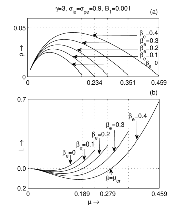
Figure 2: (a) $p$ is plotted against $\mu$ and (b) $L$ is plotted against $\mu$ for different values of $\beta_{e}$ with $B_{1}=0.001$, $\gamma=3$, $\sigma_{ie}=\sigma_{pe}=0.9$

In figure 1(b), $L$ is plotted against $\mu$ for different values of $\beta_{e}$ with $\gamma=3$, $\sigma_{ie}=\sigma_{pe}=0.9$ when $B_{1}=0.00001$, i.e., in figure 1(b), L is plotted against $\mu$ along the each curve of figure 1(a). Figure 1(b) clearly shows that there exists a value $\mu_{cr}$ of $\mu$ such that $L>0$ or $L<0$ according to whether $\mu>\mu_{cr}$ or $\mu<\mu_{cr}$ and $L=0$ at $\mu=\mu_{cr}$. Obviously, in the small neighbourhood of $\mu=\mu_{cr}$, $L$ is close to zero. Again, for each $\beta_{e}$ lying within a fixed interval, there exists a value $\mu_{cr}$ of $\mu$ such that $L=0$. So, for $L=0$, we can use the DL solution (38) as the solution of the combined MKP-KP equation (1). In this connection, we want to mention the following point of Sardar et al. Sardar, Bandyopadhyay, and Das (2016a) Sardar et al. Sardar, Bandyopadhyay, and Das (2016a) reported that the alternative solitary wave solution of the combined MKP - KP equation (1) cannot describe the nonlinear behaviour of DIA waves when $L=0$ or $L\approx O(\epsilon)$ and further investigation is necessary when $L=0$ or $L\approx O(\epsilon)$.

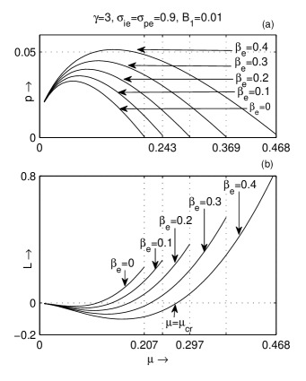
Figure 3: (a) $p$ is plotted against $\mu$ and (b) $L$ is plotted against $\mu$ for different values of $\beta_{e}$ with $B_{1}=0.01$, $\gamma=3$, $\sigma_{ie}=\sigma_{pe}=0.9$

Similarly, figure 2(a) shows the existence of a region in the parameter space where $B_{1}=0.001$ and figure 2(b) shows the existence of the points $\mu_{cr}$ of $\mu$ such that $L=0$ at $\mu=\mu_{cr}$. Figure 3(a) shows the existence of a region in the parameter space where $B_{1}=0.01$ and figure 3(b) shows the existence of the points $\mu_{cr}$ of $\mu$ such that $L=0$ at $\mu=\mu_{cr}$. Sardar et al. Sardar, Bandyopadhyay, and Das (2016a) have already drawn the existence of a region in the parameter space where $B_{1}=0.0001$ in figure 2(a) whereas in figure 2(b), they have drawn the the existence of the points $\mu_{cr}$ of $\mu$ such that $L=0$ at $\mu=\mu_{cr}$ for $B_{1}=0.0001$. From the above mentioned figures, we can conclude that we can draw the existence of a region in the parameter space for any given small value of $B_{1}$ and for this value of $B_{1}$, we can easily find the existence of the point $\mu_{cr}$ of $\mu$ such that $L=0$ at $\mu=\mu_{cr}$ for any fixed value of $\beta_{e}$ and for different values of $\beta_{e}$, one can get different $\mu_{cr}$ such that $L=0$ at $\mu=\mu_{cr}$. So, in the present paper, we are able to give a consistent solution of the combined MKP - KP equation (1) when $L=0$.

The solution (38) is the steady state solution of the combined MKP - KP equation (1) along the $x$ - axis. This solution is same as the DL solution of the combined MKdV - KdV equation corresponding to the combined MKP - KP equation (1), i.e., the steady state solitary wave solution of the combined MKdV - KdV equation

$$\phi^{(1)}_{\tau}+AB_{1}\phi^{(1)}\phi^{(1)}_{\xi}+AB_{2}(\phi^{(1)})^{2}\phi^{(1)}_{\xi}+\frac{1}{2}AC\phi^{(1)}_{\xi\xi\xi}=0.$$ (44)

is exactly same as the equation (38). In the present paper, we have considered the lowest order transverse stability of the DL solution of the combined MKdV - KdV equation (44) using the three-dimensional combined MKP - KP equation (1). In fact, to study the transverse stability of the DL solution of the combined MKdV - KdV equation (44), we have considered the three-dimensional combined MKP - KP equation (1) by taking the weak dependence of the spatial coordinates perpendicular to the direction of propagation of the wave.

IV Stability analysis

In section III, we have seen that the equation (38) gives two different DL solutions of the combined MKP-KP equation (1) for two different values of $\lambda$, viz., $\lambda=+1$ and $\lambda=-1$. In this section, we have considered the stability analysis of the double layer solution (38) for $\lambda=+1$. Following the same procedure, one can easily analyse the stability of the DL solution (38) for $\lambda=-1$.

To analyze the stability of the DL solution (38) of the equation (11) by the multiple-scale perturbation expansion method of Allen and Rowlands Allen and Rowlands (1993, 1995), we decompose $\phi^{(1)}$ as

$$\phi^{(1)}=\phi_{0}(X)+q(X,\eta,\zeta,\tau),$$ (45)

where $\phi_{0}(X)$ is the DL solution (38) of the equation (11) and $q(X,\eta,\zeta,\tau)$ is the perturbed part of $\phi^{(1)}$. Substituting (45) into (11) and linearizing this equation with respect to $q$ we get the following equation:

$$q_{X\tau}+\Big{(}M_{1}q\Big{)}_{XX}+\frac{1}{2}AD(q_{\eta\eta}+q_{\zeta\zeta})=0,$$ (46)

where

$$M_{1}=-U+AB_{1}\phi_{0}+AB_{2}\phi_{0}^{2}+\frac{1}{2}AC\frac{\partial^{2}}{\partial X^{2}}$$ (47)

and we have used the following notations:

$$q_{X\tau}=\frac{\partial^{2}q}{\partial X\partial\tau}~{},~{}\Big{(}M_{1}q\Big{)}_{XX}=\frac{\partial^{2}}{\partial X^{2}}\Big{(}M_{1}q\Big{)}.$$ (48)

Now, for long-wavelength plane-wave perturbation along a direction having direction cosines ( $l$, $m$, $n$), we set

$$q(X,\eta,\zeta,\tau)=\overline{q}(X)e^{i\{k(lX+m\eta+n\zeta)-\omega\tau\}},$$ (49)

where $k$ is small and $l^{2}+m^{2}+n^{2}=1$.

Substituting the expression of $q(=q(X,\eta,\zeta,\tau))$ as given in (49) into the equation (46), we get the following equation of $\overline{q}$:

$$(M_{1}\overline{q})_{XX}-i\omega\overline{q}_{X}+kl\Big{\{}\omega\overline{q}+2i(M_{1}\overline{q})_{X}+iAC\overline{q}_{XXX}\Big{\}}$$

$$-k^{2}l^{2}\Big{\{}M_{1}\overline{q}+\frac{5}{2}AC\overline{q}_{XX}+AD\frac{m^{2}+n^{2}}{2l^{2}}\overline{q}\Big{\}}-k^{3}l^{3}\Big{\{}2iAC\overline{q}_{X}\Big{\}}+k^{4}l^{4}\Big{\{}\frac{1}{2}AC\overline{q}\Big{\}}=0,$$

Following the multiple-scale perturbation expansion method of Allen and Rowlands Allen and Rowlands (1993, 1995), we expand $\overline{q}(X)$ and $\omega$ as

$$\overline{q}(X)=\sum_{j=0}^{\infty}k^{j}q^{(j)}(X,X_{1},X_{2},X_{3},...),$$ (51)

$$\omega=\sum_{j=0}^{\infty}k^{j}\omega^{(j)},$$ (52)

where $\omega^{(0)}=0$, $X_{j}=k^{j}X$, $j=0,1,2,3...,$ and each $q^{(j)}(=q^{(j)}(X,X_{1},X_{2},X_{3},...))$ is a function of $X,X_{1},X_{2},X_{3},\cdots$ . It is important to note that $X_{0}=X$.

Finally, substituting (51) and (52) into the equation (IV) and then equating the coefficients of different powers of $k$ on the both sides of the resulting equation, we get the following sequence of equations:

$$\frac{\partial}{\partial X}(M_{1}q^{(j)})=Q^{(j)},$$ (53)

where

$$Q^{(j)}=\int_{\infty}^{X}{R^{(j)}}dX,$$ (54)

and the expression of $R^{(j)}$ for $j$ = $0$ and $1$ are given in the following equations:

$$R^{(0)} = 0,$$ (55)

$$R^{(1)} = i\omega^{(1)}q^{(0)}_{0}-iAClq^{(0)}_{000}-ACq^{(0)}_{0001}-2il[M_{1}q^{(0)}]_{0}-2[M_{1}q^{(0)}]_{01}.$$ (56)

Here, we have used the following notations:

$$q^{(j)}_{r}=\frac{\partial q^{(j)}}{\partial X_{r}},~{}q^{(j)}_{rs}=\frac{\partial^{2}q^{(j)}}{\partial X_{r}\partial X_{s}},~{}q^{(j)}_{rst}=\frac{\partial^{3}q^{(j)}}{\partial X_{r}\partial X_{s}\partial X_{t}}$$

$$q^{(j)}_{rsty}=\frac{\partial^{4}q^{(j)}}{\partial X_{r}\partial X_{s}\partial X_{t}\partial X_{y}},~{}[M_{1}q^{(j)}]_{rs}=\frac{\partial^{2}(M_{1}q^{(j)})}{\partial X_{r}\partial X_{s}}$$

Assuming that $q^{(j)}$ and its derivative up to third order vanish as $X\rightarrow\infty$, the general solution of (53) can be written as

$$q^{(j)} = A^{(j)}_{1}f+A^{(j)}_{2}f\int\frac{1}{f^{2}}dX+A^{(j)}_{3}f\int\frac{\phi_{0}}{f^{2}}dX+\frac{2}{AC}f\int\frac{\int(f\int Q^{(j)}dX)dX}{f^{2}}dX,$$

where $\displaystyle f=\frac{d\varphi_{0}}{dX}$, $\phi_{0}$ is given by (38) for $\lambda=1$ and $A_{1}^{(j)},A_{2}^{(j)},A_{3}^{(j)}$ are all arbitrary functions of $X_{1},X_{2},X_{3},\cdots$.

Using MATHEMATICA Wolfram (1999), the solution (IV) for $\lambda=+1$ can be put in the following form:

$$q^{(j)} = A_{1}^{(j)}f+\frac{3W_{1}^{2}}{8a^{2}}\Big{(}A_{2}^{(j)}+aA_{3}^{(j)}\Big{)}fX+\frac{3W_{1}^{2}}{8a^{2}}\Big{(}A_{2}^{(j)}+aA_{3}^{(j)}\Big{)}\phi_{0}$$ (58)

$$+ \frac{W_{1}^{2}}{8a}\Big{(}A_{2}^{(j)}+aA_{3}^{(j)}\Big{)}e^{-\frac{2X}{W_{1}}}-\frac{W_{1}^{2}}{4a}{A_{2}^{(j)}}\frac{1}{S^{2}}-\frac{W_{1}^{2}}{4a}\Big{(}A_{2}^{(j)}+aA_{3}^{(j)}\Big{)}$$

$$+ \frac{2}{AC}f\int\frac{\int(f\int Q^{(j)}dX)dX}{f^{2}}dX,$$

where

$$S=\mbox{sech}\frac{X}{W_{1}}.$$ (59)

IV.1 Zeroth order equation

As $R^{(0)}=0$, the solution (58) of the equation (53) for $j=0$ can be written as follows :

$$q^{(0)} = A_{1}^{(0)}f+\frac{3W_{1}^{2}}{8a^{2}}\Big{(}A_{2}^{(0)}+aA_{3}^{(0)}\Big{)}fX+\frac{3W_{1}^{2}}{8a^{2}}\Big{(}A_{2}^{(0)}+aA_{3}^{(0)}\Big{)}\phi_{0}$$ (60)

$$+ \frac{W_{1}^{2}}{8a}\Big{(}A_{2}^{(0)}+aA_{3}^{(0)}\Big{)}e^{-\frac{2X}{W_{1}}}-\frac{W_{1}^{2}}{4a}{A_{2}^{(0)}}\frac{1}{S^{2}}-\frac{W_{1}^{2}}{4a}\Big{(}A_{2}^{(0)}+aA_{3}^{(0)}\Big{)}.$$

We note that each term of $q^{(0)}$ except the fifth term $\displaystyle\Big{[}-\frac{W_{1}^{2}}{4a}{A_{2}^{(0)}}\frac{1}{S^{2}}\Big{]}$ is bounded at $X=+\infty$. Therefore, to make $q^{(0)}$ bounded at $X=+\infty$, the coefficient of $\frac{1}{S^{2}}$ in the expression of $q^{(0)}$ must be identically equal to zero and consequently we get

$$-\frac{W_{1}^{2}}{4a}{A_{2}^{(0)}}=0.$$ (61)

Now, we see that each term of $q^{(0)}$ except the last term $\displaystyle\Big{[}-\frac{W_{1}^{2}}{4a}\Big{(}A_{2}^{(0)}+aA_{3}^{(0)}\Big{)}\Big{]}$ approaches zero as $X\rightarrow+\infty$. So, to make $q^{(0)}$ consistent with the condition $q^{(0)}\rightarrow 0$ as $X\rightarrow+\infty$, we must have

$$-\frac{W_{1}^{2}}{4a}\Big{(}A_{2}^{(0)}+aA_{3}^{(0)}\Big{)}=0.$$ (62)

From equations (61) and (62), we get,

$$A_{2}^{(0)}=A_{3}^{(0)}=0.$$ (63)

Therefore $q^{(0)}$ assumes the following form:

$$q^{(0)}=A_{1}^{(0)}f=A_{1}^{(0)}\frac{d\phi_{0}}{dX}.$$ (64)

IV.2 First order equation

Using the equations (56) , (64) and MATHEMATICA Wolfram (1999), the solution (58) of the differential equation (53) for $j=1$ can be put in the following form:

$$q^{(1)} = B_{1}^{(1)}f+\Big{\{}\frac{3W_{1}^{2}}{8a^{2}}\Big{(}A_{2}^{(1)}+aA_{3}^{(1)}\Big{)}+iA_{1}^{(0)}s_{1}-\frac{\partial A_{1}^{(0)}}{\partial X_{1}}\Big{\}}fX$$ (65)

$$+ \Big{\{}\frac{3W_{1}^{2}}{8a^{2}}\Big{(}A_{2}^{(1)}+aA_{3}^{(1)}\Big{)}+iA_{1}^{(0)}\frac{\omega^{(1)}}{2U}\Big{\}}\phi_{0}$$

$$+ \Big{\{}\frac{W_{1}^{2}}{8a}\Big{(}A_{2}^{(1)}+aA_{3}^{(1)}\Big{)}++iA_{1}^{(0)}\frac{a\omega^{(1)}}{2U}\Big{\}}e^{-\frac{2X}{W_{1}}}$$

$$- \frac{W_{1}^{2}}{4a}{A_{2}^{(1)}}\frac{1}{S^{2}}-\frac{W_{1}^{2}}{4a}\Big{(}A_{2}^{(1)}+aA_{3}^{(1)}\Big{)},$$

where

$$B_{1}^{(1)}=A_{1}^{(1)}+iA_{1}^{(0)}\frac{3W_{1}}{8U}\omega^{(1)},$$ (66)

$$s_{1}=\frac{\omega^{(1)}-2lU}{2U}.$$ (67)

We note that each term of $q^{(1)}$ except the fifth term $\displaystyle\Big{[}-\frac{W_{1}^{2}}{4a}{A_{2}^{(1)}}\frac{1}{S^{2}}\Big{]}$ is bounded at $X=+\infty$. Therefore, to make $q^{(1)}$ bounded at $X=+\infty$, the coefficient of $\frac{1}{S^{2}}$ in the expression of $q^{(1)}$ must be identically equal to zero and consequently we get

$$-\frac{W_{1}^{2}}{4a}{A_{2}^{(1)}}=0.$$ (68)

Now, we see that each term of $q^{(1)}$ except the last term $\displaystyle\Big{[}-\frac{W_{1}^{2}}{4a}\Big{(}A_{2}^{(1)}+aA_{3}^{(1)}\Big{)}\Big{]}$ approaches zero as $X\rightarrow+\infty$. So, to make $q^{(1)}$ consistent with the condition $q^{(1)}\rightarrow 0$ as $X\rightarrow+\infty$, we must have

$$-\frac{W_{1}^{2}}{4a}\Big{(}A_{2}^{(1)}+aA_{3}^{(1)}\Big{)}=0.$$ (69)

From equations (68) and (69), we get,

$$A_{2}^{(1)}=A_{3}^{(1)}=0.$$ (70)

Therefore $q^{(1)}$ assumes the following form:

$$q^{(1)}=B_{1}^{(1)}f+\Big{(}iA_{1}^{(0)}s_{1}-\frac{\partial A_{1}^{(0)}}{\partial X_{1}}\Big{)}fX+iA_{1}^{(0)}\frac{\omega^{(1)}}{2U}\phi_{0}+iA_{1}^{(0)}\frac{a\omega^{(1)}}{2U}e^{-\frac{2X}{W_{1}}}.$$ (71)

Now, we can remove the first term in the above expression of $q^{(1)}$ as this type of term has already been included in the lowest order term $q^{(0)}$. The second term in the above expression of $q^{(1)}$ is known as ghost secular term and this term can be removed by choosing

$$\frac{\partial A_{1}^{(0)}}{\partial X_{1}}=iA_{1}^{(0)}s_{1}.$$ (72)

Therefore, the equation (71) can be written as

$$q^{(1)} = iA_{1}^{(0)}\frac{\omega^{(1)}}{2U}\phi_{0}+iA_{1}^{(0)}\frac{a\omega^{(1)}}{2U}e^{-\frac{2X}{W_{1}}}.$$ (73)

Now we see that the first term of $q^{(1)}$ is bounded at $X=\pm\infty$ but the second term of $q^{(1)}$ is not bounded at $X=-\infty$ because of the presence of the term $e^{-\frac{2X}{W_{1}}}$. To make $q^{(1)}$ bounded at $X=-\infty$, We must have

$$iA_{1}^{(0)}\frac{a\omega^{(1)}}{2U}=0.$$ (74)

The equation (74) gives the following expression for $\omega^{(1)}$:

$$\omega^{(1)}=0.$$ (75)

Equation (75) shows that $\omega^{(1)}$ is real and consequently, the DL solution (38) for $\lambda=1$ is stable at the order $k$, where $k$ is the wave number of the perturbation.

V Conclusions

In the present paper, we have considered the problem of existence and stability of the DL solution of the combined MKP-KP equation. Analytically, we have proved that the DL solution having a profile of the form (38) of the combined MKP-KP equation exists if $L=0$. The form of the double layer solution as given by the equation (38) also suggests that there are two types of double layer solutions corresponding to two different values of $\lambda$ ($\lambda=+1$ and $\lambda=-1$). We have stated earlier that these double layer solutions of the combined MKP-KP equation are exactly same as those of the combined MKdV-KdV equation but here we consider the combined MKP-KP equation to study the stability of the double layer solutions of the corresponding combined MKdV-KdV equation. Finally, we have found that double layers are stable up to the lowest order of the wave number. We have the following differences between the paper of Sardar et al. Sardar, Bandyopadhyay, and Das (2016a) and the present paper:

• (1) In the paper of Sardar et al. Sardar, Bandyopadhyay, and Das (2016a), the method of Malfliet and Hereman Malfliet and Hereman (1996) has been used to find the alternative solitary wave solution of the combined MKP-KP equation having profile different from $\mbox{sech}^{2/r}$ for any strictly positive real value of $r$ whereas in the present paper, following the tan-hyperbolic method of Malfliet and Hereman Malfliet and Hereman (1996), we have found the double layer solution of the same combined MKP-KP equation.

• (2) In the paper of Sardar et al. Sardar, Bandyopadhyay, and Das (2016a), they have used the following boundary conditions:

  $$\phi_{0},\frac{d^{n}\phi_{0}}{dX^{n}}\to 0\mbox{ as }|X|\to\infty$$

  $\mbox{ for }n=1,2,3,\cdots$ to get the alternative solitary wave solution of the combined MKP-KP equation whereas in present paper, we have used the following conditions: either $\displaystyle\phi_{0},\frac{d^{n}\phi_{0}}{dX^{n}}\to 0\mbox{ as }X\to\infty$ or $\displaystyle\phi_{0},\frac{d^{n}\phi_{0}}{dX^{n}}\to 0\mbox{ as }X\to-\infty$ $\mbox{ for }n=1,2,3,\cdots$ to get a double layer solution of the same combined MKP-KP equation.

• (3) In the paper of Sardar et al. Sardar, Bandyopadhyay, and Das (2016a), they got the following alternative solitary wave solution of the combined MKP-KP equation:

  $$\phi_{0}=12Cp_{1}^{2}\frac{sech[2p_{1}X]}{B_{1}sech[2p_{1}X]+\lambda\sqrt{L}},$$

  where $\lambda=\pm 1$, $L=B_{1}^{2}+12B_{2}Cp_{1}^{2}>0$ and $p_{1}=\frac{1}{W_{1}}$, whereas in the present paper, we get the following double layer solution of the same combined MKP-KP equation:

  $$\phi_{0}=a\bigg{(}1-\lambda\tanh\frac{X}{W_{1}}\bigg{)},$$

  where $a=-\frac{B_{1}}{2B_{2}}$.

  Here $\lambda=1$ if we use the conditions $\phi_{0},\frac{d^{n}\phi_{0}}{dX^{n}}\to 0\mbox{ as }X\to\infty$ and $\lambda=-1$ if we use the conditions $\phi_{0},\frac{d^{n}\phi_{0}}{dX^{n}}\to 0\mbox{ as }X\to-\infty$ $\mbox{ for }n=1,2,3,\cdots$ .

• (4) In the paper of Sardar et al. Sardar, Bandyopadhyay, and Das (2016a), it has been shown that the alternative solitary wave solution of the combined MKP-KP equation exists only when $L>0$ whereas in the present paper, it has been shown that the double layer solution of the same combined MKP-KP equation exists when $L=0$.

• (5) In the paper of Sardar et al. Sardar, Bandyopadhyay, and Das (2016a), it has been shown that the alternative solitary wave solution of the combined MKP-KP equation converges to the solitary wave solution of MKP equation when $B_{1}\rightarrow 0$ whereas in the present paper, we see that the double layer solution of the same combined MKP-KP equation does not converge to the solitary wave solution of the MKP equation when $B_{1}\rightarrow 0$ and it is impossible to get any double layer solution of the MKP equation.

Regarding stability analysis, we want to mention that we have used the small-$k$ perturbation expansion method of Rowlands and Infeld Rowlands (1969); Infeld (1972); Infeld and Rowlands (1973); Zakharov and Rubenchik (1974); Infeld (1985) to analyse the lowest order stability of the alternative solitary wave solution of the combined MKP-KP equation whereas we have used the multiple-scale perturbation expansion method of Allen and Rowlands Allen and Rowlands (1993) to analyse the lowest order stability of the double layer solution of the combined MKP-KP equation. In fact, one cannot use the small-$k$ perturbation expansion method of Rowlands and Infeld Rowlands (1969); Infeld (1972); Infeld and Rowlands (1973); Zakharov and Rubenchik (1974); Infeld (1985) to analyse the lowest order stability of double layer solution of the combined MKP-KP equation.

References

- Block (1972) L. P. Block, Cosm. Electrodyn. 3, 349 (1972).
- Mozer et al. (1977) F. S. Mozer, C. W. Carlson, M. K. Hudson, R. B. Torbert, B. Parady, J. Yatteau, and M. C. Kelley, Phys. Rev. Lett. 38, 292 (1977).
- Sato and Okuda (1980) T. Sato and H. Okuda, Phys. Rev. Lett. 44, 740 (1980).
- Hudson and Potter (1981) M. K. Hudson and D. W. Potter, In Phys. of Auroral Arc formation 25, 260 (1981).
- Temerin et al. (1982) M. Temerin, K. Cerny, W. Lotko, and F. S. Mozer, Phys. Rev. Lett. 48, 1175 (1982).
- Schamel (1986) H. Schamel, Phys. Rep 140, 161 (1986).
- Kim (1987) K. Y. Kim, Phys. Fluids 30, 3686 (1987).
- Schamel (1987) H. Schamel, Z. Naturforsch., A: Phys. Sci. 42a, 1167 (1987).
- Boström et al. (1988) R. Boström, G. Gustafsson, B. Holback, G. Holmgren, H. Koskinen, and P. Kintner, Phys. Rev. Lett. , 82 (1988).
- Boström (1992) R. Boström, IEEE Trans. Plasma Sci. 20, 756 (1992).
- Han and Kim (1994) J. M. Han and K. Y. Kim, Plasma Phys. Control. Fusion 36, 1141 (1994).
- Dovner et al. (1994) P. O. Dovner, A. I. Eriksson, R. Boström, and B. Holback, Geophy. Res. Lett. 21, 1827 (1994).
- Mozer and Kletzing (1998) F. S. Mozer and C. A. Kletzing, Geophys. Res. Lett. 25, 1629 (1998).
- Ergun et al. (2002) R. E. Ergun, L. Andersson, D. S. Main, Y. J. Su, C. W. Carlson, J. P. McFadden, and F. S. Mozer, Phys. Plasmas 9, 3685 (2002).
- Main, Newman, and Ergun (2006) D. S. Main, D. L. Newman, and R. E. Ergun, Phys. Rev. Lett. 97, 185001 (2006).
- Kim et al. (2007) T. H. Kim, S. S. Kim, H. Y. Kim, and J. H. Hwang, J. Plasma Phys. 73, 485 (2007).
- Angelopoulos (2008) V. Angelopoulos, Space Sci Rev 141, 5–43 (2008).
- Ergun et al. (2009) R. E. Ergun, L. Andersson, J. Tao, V. Angelopoulos, J. Bonnell, J. P. McFadden, D. E. Larson, S. Eriksson, T. Johansson, C. M. Cully, et al., Phys. Rev. Lett. 102, 155002 (2009).
- Li et al. (2015) S. Y. Li, S. F. Zhang, H. Cai, X. B. Bai, and Q. H. Xie, Sci China Earth Sci 58, 562 (2015).
- Coakley and Hershkowitz (1979) P. Coakley and N. Hershkowitz, Phys. Fluids 22, 1171 (1979).
- Leung, Wong, and Quon (1980) P. Leung, A. Y. Wong, and B. H. Quon, Phys. Fluids 23, 992 (1980).
- Stenzel, Ooyama, and Nakamura (1980) R. L. Stenzel, M. Ooyama, and Y. Nakamura, Phys. Rev. Lett. 45, 1498 (1980).
- Sato et al. (1981) N. Sato, R. Hatakeyama, S. Iizuka, T. Mieno, K. Saeki, J. J. Rasmussen, and P. Michelsen, Phys Rev Lett. 46, 1330 (1981).
- (24) N. Sato, in Symposium on Plasma Double Layers, Risø National Laboratory June 16-18, 1982, p. 116.
- Sato et al. (1983) N. Sato, R. Hatakeyama, S. Iizuka, T. Mieno, K. Saeki, J. J. Rasmussen, P. Michelsen, and R. Schrittwieser, J. Phys. Soc. Jpn. 52, 875 (1983).
- (26) Y. Nakamura and R. L. Stenzel, in Symposium on Plasma Double Layers, Risø National Laboratory June 16-18, 1982, p. 153.
- Torvén and Andersson (1979) S. Torvén and D. Andersson, J. Phys. D 12, 717 (1979).
- Torvén and Lindberg (1980) S. Torvén and L. Lindberg, J. Phys. D 13, 2285 (1980).
- Baker et al. (1981) K. D. Baker, N. Singh, L. P. Block, R. Kist, W. Kampa, and H. Thiemann, J. Plasma Phys. 26, 1 (1981).
- Jovanović et al. (1982) D. Jovanović, J. P. Lynov, P. Michelsen, H. L. Pecseli, J. J. Rasmussen, and K. Thomsen, Geophys. Res. Lett. 9, 1049 (1982).
- Mozer et al. (1980) F. S. Mozer, C. A. Cattell, M. K. Hudson, R. L. Lysak, M. Temerin, and R. B. Torbert, Space Sci. Rev. 27, 155 (1980).
- Sato and Okuda (1981) T. Sato and H. Okuda, J. Geophys. Res. 86, 3357 (1981).
- Bharuthram and Shukla (1986) R. Bharuthram and P. K. Shukla, Phys. Fluids 29, 3214 (1986).
- Bandyopadhyay and Das (2000) A. Bandyopadhyay and K. P. Das, Phys. Scr. 61, 92 (2000).
- Bandyopadhyay and Das (2001) A. Bandyopadhyay and K. P. Das, Phys. Scr. 63, 145 (2001).
- Ghosh and Bharuthram (2008) S. Ghosh and R. Bharuthram, Astrophys. Space Sci. 314, 121 (2008).
- Ourabah and Tribeche (2013) K. Ourabah and M. Tribeche, Astrophys. Space Sci. 348, 511 (2013).
- Alam, Masud, and Mamun (2014) M. S. Alam, M. M. Masud, and A. A. Mamun, Astrophys. Space Sci. 349, 245 (2014).
- Masud, Tasnim, and Mamun (2015) M. M. Masud, I. Tasnim, and A. A. Mamun, Pramana 84, 137 (2015).
- Allen and Rowlands (1993) M. A. Allen and G. Rowlands, J. Plasma Phys. 50, 413 (1993).
- Sardar, Bandyopadhyay, and Das (2016a) S. Sardar, A. Bandyopadhyay, and K. P. Das, Phys. Plasmas 23, 123706 (2016a).
- Sardar, Bandyopadhyay, and Das (2016b) S. Sardar, A. Bandyopadhyay, and K. P. Das, Phys. Plasmas 23, 073703 (2016b).
- Cairns et al. (1995) R. A. Cairns, A. A. Mamum, R. Bingham, R. Boström, R. O. Dendy, C. M. C. Nairn, and P. K. Shukla, Geophys. Res. Lett. 22, 2709 (1995).
- Malfliet and Hereman (1996) W. Malfliet and W. Hereman, Phys. Scr. 54, 563 (1996).
- Allen and Rowlands (1995) M. A. Allen and G. Rowlands, J. Plasma Phys. 53, 63 (1995).
- Wolfram (1999) S. Wolfram, The MATHEMATICA® book, version 4 (Cambridge university press, 1999).
- Rowlands (1969) G. Rowlands, J. Plasma Phys. 3, 567 (1969).
- Infeld (1972) E. Infeld, J. Plasma Phys. 8, 105 (1972).
- Infeld and Rowlands (1973) E. Infeld and G. Rowlands, J. Plasma Phys. 10, 293 (1973).
- Zakharov and Rubenchik (1974) V. E. Zakharov and A. M. Rubenchik, Sov. Phys. - JETP 38, 494 (1974).
- Infeld (1985) E. Infeld, J. Plasma Phys. 33, 171 (1985).