A space-time pseudospectral discretization method for solving diffusion optimal control problems
with two-sided fractional derivatives

Abstract

We propose a direct numerical method for the solution of an optimal control problem governed by a two-side space-fractional diffusion equation. The presented method contains two main steps. In the first step, the space variable is discretized by using the Jacobi–Gauss pseudospectral discretization and, in this way, the original problem is transformed into a classical integer-order optimal control problem. The main challenge, which we faced in this step, is to derive the left and right fractional differentiation matrices. In this respect, novel techniques for derivation of these matrices are presented. In the second step, the Legendre–Gauss–Radau pseudospectral method is employed. With these two steps, the original problem is converted into a convex quadratic optimization problem, which can be solved efficiently by available methods. Our approach can be easily implemented and extended to cover fractional optimal control problems with state constraints. Five test examples are provided to demonstrate the efficiency and validity of the presented method. The results show that our method reaches the solutions with good accuracy and a low CPU time.

1 Introduction

Fractional (non-integer order) order diffusion equations, in comparison with classical integer order counterparts, can describe more accurately irregular diffusion processes, such as gas diffusion in fractal porous media and heat conduction (Wu et al., 2015, 2017; Yang et al., 2017b; Yang and Machado, 2017). Accordingly, the numerical solution of fractional diffusion equations has gained considerable attention (Meerschaert and Tadjeran, 2006; Doha et al., 2014; Zaky et al., 2016; Yang et al., 2017a, 2016; Feng et al., 2018; Chen et al., 2018; Yang et al., 2017c).

Optimal control of fractional diffusion equations has recently received special attention, due to their applications in various fields, such as control of temperature in a thermo conduction process or mass diffusive transport in a porous media (Du et al., 2016).

Mophou (2011) considered the optimal control of a time-fractional diffusion equation in a bounded domain and investigated the questions of existence and uniqueness of solution. Moreover, the first-order optimality conditions are derived in (Mophou, 2011).

The optimal control of time-fractional diffusion equations with state constraints and non-homogeneous Dirichlet boundary conditions is considered in Mophou and N’Guérékata (2011) and Dorville et al. (2011), respectively. In these papers, existence and uniqueness of solution and first-order optimality conditions are also studied. Regarding numerical methods for solving optimal control problems of time-fractional diffusion equations, we refer to Li and Zhou (2018); Yamamoto (2018). The reader interested on the optimal control of fractional partial differential equations is referred to Agarwal et al. (2018); Zaky and Machado (2017); Zaky (2018); Bai et al. (2018); Darehmiraki et al. (2018) and references therein.

Recently, an optimal control problem governed by a two-sided space-fractional diffusion equation was considered in Du et al. (2016) and Wu and Huang (2018). More precisely, a constrained time-dependent optimal control problem defined on the space interval $(0,1)$ and time period $[0,T]$ was considered. The aim is to find the control $u(x,t)\in L^{2}\left(0,T;(0,1)\right)$ and state $y(x,t)\in L^{2}\left(0,T;(0,1)\right)$ such that the space-fractional diffusion equation

$$\frac{\partial y}{\partial t}(x,t)=c(x,t)\left[r\,{}_{\text{\tiny 0}}\mathcal{D}_{x}^{2-\beta}y(x,t)+(1-r){}_{x}\mathcal{D}_{\text{\tiny 1}}^{2-\beta}y(x,t)\right]$$

$$+f(x,t)+u(x,t),$$ (1a)

with initial condition

$$y(x,0)=g(x),\quad x\in(0,1),$$ (1b)

and the boundary conditions

$$y(0,t)=y(1,t)=0,\quad t\in(0,T),$$ (1c)

are satisfied and the following performance index is minimized:

$$J[u]:= \tfrac{1}{2}\int_{0}^{T}\int_{0}^{1}\big{[}y(x,t)-z(x,t)\big{]}^{2}\text{d}x\text{d}t$$

$$\qquad+\tfrac{1}{2}\int_{0}^{T}\int_{0}^{1}u^{2}(x,t)\text{d}x\text{d}t.$$ (1d)

Moreover, the following constraint on the control function is considered:

$$u(x,t)\geq u_{\min}(x,t),\quad x\in(0,1),\ t\in(0,T),$$ (1e)

where $$u_{\min}$$ is a known function.

In problem (1), $z(x,t)$ is a known function, which represents the observed or desired values of state function $y$, $f(x,t)$ is the source or sink term, $d(x,t)$ is the diffusivity coefficient and $2-\beta$ is the order of diffusion, where $0<\beta<1$. Moreover, ${}_{\text{\tiny 0}}\mathcal{D}_{x}^{2-\beta}$ and ${}_{x}\mathcal{D}_{\text{\tiny 1}}^{2-\beta}$ denote the left and right Riemann–Liouville fractional derivatives, defined (see, e.g., Malinowska and Torres (2012)) as

$${}_{\text{\tiny 0}}\mathcal{D}_{x}^{\alpha}g(x)=\dfrac{1}{\Gamma(2-\alpha)}\dfrac{\text{d}^{2}}{\text{d}x^{2}}\int_{0}^{x}{(x-s)}^{1-\alpha}g(s)\text{d}s.$$

$${}_{x}\mathcal{D}_{\text{\tiny 1}}^{\alpha}g(x)=\dfrac{1}{\Gamma(2-\alpha)}\dfrac{\text{d}^{2}}{\text{d}x^{2}}\int_{s}^{1}{(s-x)}^{1-\alpha}g(s)\text{d}s.$$

Generally speaking, the two main challenges in solving problem (1) numerically are: (i) the problem contains both left and right fractional derivatives, (ii) the fractional derivatives are nonlocal and singular operators. Moreover, when using finite-difference-based methods, the stiffness of the approximation matrix of the fractional derivative is added to the two aforementioned drawbacks (Wu and Huang, 2018). Thus, finite difference schemes, for solving problem (1), require expensive computation time and storage cost. In this regard, the main concern in the finite difference based methods for solving the problem (1) is to reduce the demand for time and memory computation (Du et al., 2016; Wu and Huang, 2018). In Du et al. (2016), necessary optimality conditions for problem (1) are derived and a faithful and fast gradient projection method is developed to solve them numerically. In Wu and Huang (2018), to get more reduction of computational times, a parallel-in-time algorithm for implementing the gradient projection method is presented for problem (1).

In this paper, we present another method for solving problem (1) numerically. There are two major differences between the method we propose here and the ones of Du et al. (2016) and Wu and Huang (2018). First, our approach is based on high-order and global pseudospectral methods rather than finite difference schemes. Second, our method is direct, that is, does not rely on necessary optimality conditions. In a direct method, the optimal control problem is solved by transcribing it into a Non-Linear Programming (NLP) problem; thereafter, an NLP-solver is used to solve the resulting NLP problem (Pooseh et al., 2013; Salati et al., 2019; Behroozifar and Habibi, 2018; Mashayekhi and Razzaghi, 2018). The direct methods are easily implemented and inequality constraints on state and control are handled simpler, in comparison with indirect methods (Pooseh et al., 2013; Salati et al., 2019; Mohammadzadeh et al., 2018).

Pseudospectral methods approximate the unknown function(s) using interpolating polynomials with specific collocation points such as Legendre–Gauss (LG) (Benson et al., 2006), Legendre–Gauss–Lobatto (LGL) (Elnagar et al., 1995) and Legendre–Gauss–Radau (LGR) points (Garg et al., 2010). These selections lead to the three most common types of pseudospectral methods, which are referred as LG pseudospectral (Benson et al., 2006), LGL pseudospectral (Fahroo and Ross, 2001; Elnagar et al., 1995), and LGR pseudospectral (Garg, 2011; Garg et al., 2010) methods.

It is a well-known fact that, to solve ordinary or partial differential equations with a simple domain and a smooth solution, pseudospectral methods can usually achieve an accurate solution even with a small number of nodes. On the other hand, for problems with a non-smooth solution, the accuracy of pseudospectral methods is reduced. However, for problems with a non-smooth solution, they lead to a reasonably accurate approximation with less demand on computational time and computer memory.

Due to the mentioned computational efficiency, pseudospectral methods have been popular for the numerical solution of optimal control problems governed by integer order differential equations (Garg et al., 2010; Foroozandeh et al., 2017; Ezz-Eldien et al., 2017; Foroozandeh et al., 2018). More recently, pseudospectral methods have been extended for solving optimal control problems governed by fractional ordinary and partial differential equations (Tang et al., 2017; Li and Zhou, 2018; Khaksar-e Oshagh and Shamsi, 2017).

Here we present a direct method for solving problem (1) that consists in two steps. In the first step, the Jacobi–Gauss pseudospectral method is used for space discretization and, as a result, the problem is reduced to a classical optimal control problem. It is worthwhile to note that, because of the existence of both left and right space-fractional derivatives in the considered problem, we need to compute the left and right fractional differentiation matrices. These differentiation matrices, which are approximations of the left and right fractional operators, play an important role in the pseudospectral method and, therefore, need to be obtained accurately. In this paper, by using some useful properties of the Jacobi polynomials, we present efficient strategies for computing the left and right fractional differentiation matrices. In the second step of our method, we apply the Legendre–Gauss–Radau pseudospectral method. The resulting ordinary optimal control problem is then transcribed into a quadratic optimization problem. In addition, for easy implementation and analysis, the standard form of the quadratic optimization problem is derived.

The rest of the paper is organized as follows. In section “Preliminaries and notations”, we recall some necessary definitions and relevant properties of the Jacobi polynomials, quadrature rules, and the Kronecker product. Next section is devoted to the first step of our method, where the Jacobi–Gauss pseudospectral method is applied for space discretization of the problem. Moreover, the computation of the differentiation matrices is presented in this section. Then the second step of our method is presented, where the Legendre–Gauss–Radau pseudospectral method is utilized to reduce the problem to a quadratic optimization one. In section “Numerical experiments”, five illustrative examples are investigated to assess the accuracy and efficiency of the proposed numerical method. We end with a section of conclusions.

2 Preliminaries and notations

Jacobi polynomials have great flexibility to develop efficient numerical methods for solving a wide range of fractional differential models. Consequently, in the last decade, Jacobi polynomials have been widely used to solve fractional problems (Esmaeili and Shamsi, 2011; Esmaeili et al., 2011; Bhrawy and Zaky, 2015; Dehghan et al., 2016; Bhrawy and Zaky, 2016; Zaky et al., 2018). Our method uses Jacobi polynomials too. Thus, in this section we briefly review the Jacobi polynomials, Jacobi quadrature rules, and some relevant theorems on the derivatives of Jacobi polynomials.

2.1 Jacobi Polynomials

The Jacobi polynomials $P_{n}^{(a,b)}(\tau)$, where $\tau\in[-1,1]$ and $n=0,1,\ldots$, are given explicitly by Gautschi (1996):

$$P_{n}^{(a,b)}(\tau)=\tfrac{1}{2^{n}}\sum_{k=0}^{n}\begin{pmatrix}n+a\\ n-k\end{pmatrix}\begin{pmatrix}n+b\\ k\end{pmatrix}(\tau-1)^{k}(\tau+1)^{n-k}.$$

However, in practice, one can use the so-called recurrence Bonnet’s relation to generate the Jacobi polynomials in a stable and accurate manner (Gautschi, 1996). If $a,b>-1$, Jacobi polynomials are called classical Jacobi polynomials. The well-known Legendre polynomials are a special case of the Jacobi polynomials when $a=b=0$. In the following, some useful properties of the classical Jacobi polynomials are reviewed.

The classical Jacobi polynomials are orthogonal on the canonical interval $[-1,1]$ with respect to the weight function $(1-\tau)^{a}(1+\tau)^{b}$, i.e.,

$$\int_{-1}^{1}(1-\tau)^{a} (1+\tau)^{b}P_{n}^{(a,b)}(\tau)P_{m}^{(a,b)}(\tau)d\tau$$

$$=\begin{cases}0,&m\neq n,\\ \frac{2^{a+b+1}\Gamma(n+a+1)\Gamma(n+b+1)}{n!(2n+a+b+1)\Gamma(n+a+b+1)},&m=n.\end{cases}$$ (2)

A useful formula that relates the Jacobi polynomials and their derivatives is

$$\frac{d^{k}}{d\tau^{k}}P_{n}^{(a,b)}(\tau)=\frac{\Gamma(k+n+a+b+1)}{2^{k}\Gamma(n+a+b+1)}P_{n-k}^{(a+k,b+k)}(\tau),$$

$$\quad\qquad n\geq k.$$

The Jacobi polynomials also satisfy the following properties:

$$P_{k}^{(a,b-1)}(2x-1)= \tfrac{k+a+b}{2k+a+b}P_{k}^{(a,b)}(2x-1)$$

$$\ \ +\tfrac{k+a}{2k+a+b}P_{k-1}^{(a,b)}(2x-1),$$ (3)

$$P_{k}^{(a-1,b)}(2x-1)= \tfrac{k+a+b}{2k+a+b}P_{k}^{(a,b)}(2x-1)$$

$$\ \ -\tfrac{k+b}{2k+a+b}P_{k-1}^{(a,b)}(2x-1).$$ (4)

In the following, we recall two important theorems, which are used later to establish our method.

Theorem 1 (See Zayernouri and Karniadakis (2013)).

Let $r-\alpha>-1$ and $q+\alpha>-1$. Then, for $x\in[0,1]$, we have:

$${}_{\text{\tiny 0}}\mathcal{D}_{x}^{\alpha}\left[x^{r}P_{k}^{(q,r)}\left({2x}-1\right)\right]$$

$$\qquad\quad=\tfrac{\Gamma(k+r+1)}{\Gamma(k+r-\alpha+1)}x^{r-\alpha}P_{k}^{(q+\alpha,r-\alpha)}\left({2x}-1\right).$$

Theorem 2 (See Zayernouri and Karniadakis (2013)).

Let $q-\alpha>-1$ and $r+\alpha>-1$. Then, for $x\in[0,1]$, we have:

$${}_{x}\mathcal{D}_{\text{\tiny 1}}^{\alpha}\left[(1-\tau)^{q}P_{k}^{(q,r)}\left({2x}-1\right)\right]$$

$$\quad\qquad=\tfrac{\Gamma(k+q+1)}{\Gamma(k+q-\alpha+1)}(1-\tau)^{r-\alpha}P_{k}^{(q-\alpha,r+\alpha)}\left({2x}-1\right).$$

2.2 Jacobi nodes and quadratures

In the pseudospectral methods, the Jacobi–Gauss and Jacobi–Gauss–Radau nodes are successfully used as discretization points (Garg et al., 2010). Here we recall the definitions of these nodes and their corresponding quadrature rules (Gautschi, 1996; Garg, 2011).

Since the Jacobi polynomials are orthogonal in $[-1,1]$, all the zeros of $P_{n}^{(a,b)}(\tau)$ are simple and belong to the interval $(-1,1)$ (Gautschi, 1996). These zeros are called the Jacobi–Gauss nodes with parameters $a$ and $b$, which we denote by $\{\xi^{(a,b)}_{i}\}_{i=1}^{n}$. The Jacobi–Gauss quadrature rule with parameters $a$ and $b$ is based on the Jacobi–Gauss nodes $\{\xi^{(a,b)}_{i}\}_{i=1}^{n}$ and can be used for approximating the integral of a function over the interval $[-1,1]$ with weight $(1-x)^{a}(1+x)^{b}$ as

$$\int_{-1}^{1}(1-x)^{a}(1+x)^{b}f(x)\text{d}x\simeq\sum_{i=1}^{n}\omega^{(a,b)}_{i}f(\xi^{(a,b)}_{i}),$$ (5)

where $\omega^{(a,b)}_{i}$, $i=1,\ldots,n$, are the Jacobi–Gauss quadrature weights. The above quadrature is exact whenever $f(x)$ is a polynomial of degree equal or less than $2n-1$, i.e., in the Jacobi–Gauss quadrature rule, the degree of exactness is $2n-1$.

In the Jacobi–Gauss–Radau nodes $\{\tau^{(a,b)}_{i}\}_{i=1}^{m}$, the first node is $\tau_{1}=-1$ and the last $m-1$ nodes are the zeros of $P^{(a,b)}_{m-2}(t)+P^{(a,b)}_{m-1}(t)$. We note that the zeros of $P^{(a,b)}_{m-2}(t)+P^{(a,b)}_{m-1}(t)$ belong to $(-1,1)$. Thus, the Jacobi–Gauss–Radau points lie in the interval $[-1,1)$. The Jacobi–Gauss–Radau quadrature rule with parameters $a$ and $b$ is given by

$$\int_{-1}^{1}(1-t)^{a}(1+t)^{b}f(t)\text{d}t\simeq\sum_{i=1}^{m}\varpi^{(a,b)}_{i}f(\tau^{(a,b)}_{i}),$$ (6)

where $\tau^{(a,b)}_{i}$, $i=1,\ldots,m$, are the Jacobi–Gauss–Lobatto quadrature weights. The degree of exactness of the Jacobi–Gauss–Radau quadrature is $2m-2$.

2.3 Kronecker products

Let $\mathbf{A}\in\mathbb{R}^{m\times n}$, $\mathbf{B}\in\mathbb{R}^{p\times q}$. The Kronecker product of matrices $\mathbf{A}$ and $\mathbf{B}$ is defined as

$$\mathbf{A}\otimes\mathbf{B}=\left[\begin{array}[]{ccc}{a}_{11}\mathbf{B}&\cdots&a_{1n}\mathbf{B}\\ \vdots&\ddots&\vdots\\ {a}_{m1}\mathbf{B}&\cdots&a_{mn}\mathbf{B}\\ \end{array}\right]\in\mathbb{R}^{mp\times nq}.$$

Theorem 3 (See Laub (2005)).

For any three matrices $\mathbf{A}$, $\mathbf{B}$ and $\mathbf{E}$, for which the matrix product $\mathbf{ABE}$ is defined, one has

$$\text{\bf{vec}}(\mathbf{ABE})=(\mathbf{R}^{T}\otimes\mathbf{A})\text{\bf{vec}}(\mathbf{B}),$$

where vec is the vectorization operator, which converts a matrix into a column vector by stacking the columns of the matrix on the top of one another.

3 Step I: The Jacobi–Gauss pseudospectral method for spatial discretization

The first step of our method consists to discretize the spatial variable $x$. For that, we use the pseudospectral method based on the Jacobi–Gauss nodes with parameters $(a,b)=(1,1)$. Let $n$ be a positive integer number. Since the spatial domain of the problem is $[0,1]$, we consider the Jacobi–Gauss nodes correspondent to the interval $[0,1]$ as

$$\hat{\xi}_{i}:=\frac{1}{2}\left(\xi^{\text{\tiny(1,1)}}_{i}+1\right),\quad i=1,\dots,n.$$ (7)

The control and state functions are approximated as

$$u(x,t)\simeq\tilde{u}_{n}(x,t):=\sum_{j=1}^{n}u_{j}(t)\ell_{j}(x),$$ (8)

$$y(x,t)\simeq\tilde{y}_{n}(x,t):=\sum_{j=1}^{n}y_{j}(t)\mathring{\ell}_{j}(x),$$ (9)

where $\ell_{j}(x)$, $j=1,\ldots,n$, are the Lagrange basis polynomials based on the Jacobi–Gauss nodes $\left\{\hat{\xi}_{i}\right\}_{i=1}^{n}$, i.e.,

$$\ell_{j}(x):=\prod_{\begin{subarray}{c}k=1\\ k\neq j\end{subarray}}^{n}\frac{x-\hat{\xi}_{k}}{\hat{\xi}_{j}-\hat{\xi}_{k}}$$ (10)

and

$$\mathring{\ell}_{j}(x):=\frac{x(1-x)}{\hat{\xi}_{j}\left(1-\hat{\xi}_{j}\right)}\ell_{j}(x).$$

Note that $\ell_{j}(x)$ and $\mathring{\ell}_{j}(x)$ satisfy the following Kronecker properties in the Jacobi–Gauss nodes:

$$\mathring{\ell}_{j}(\hat{\xi}_{i})=\ell_{j}(\hat{\xi}_{i})=\begin{cases}0\ \ if\ \ i\neq j\\ 1\ \ if\ \ i=j\end{cases},\ \ j=1,\ldots,n.$$ (11)

Moreover, $\mathring{\ell}_{j}(0)=\mathring{\ell}_{j}(1)=0$, $j=1,\ldots,n$. Therefore, for each value of $y_{j}(t)$, $j=1,\ldots,n$, the approximation $\tilde{y}_{n}(x,t)$ satisfies the boundary conditions (1c).

By substituting the approximations (8) and (9) in equation (1a), and by simple algebraic manipulation, we get

$$\sum_{j=1}^{n}\dot{y}_{j}(t)\mathring{\ell}_{j}(x)=c(x,t)\left[r\sum_{j=1}^{n}y_{j}(t){}_{\text{\tiny 0}}\mathcal{D}_{x}^{2-\beta}\mathring{\ell}_{j}(x)\right.$$

$$\left.+(1-r)\sum_{j=1}^{n}y_{j}(t){}_{x}\mathcal{D}_{\text{\tiny 1}}^{2-\beta}\mathring{\ell}_{j}(x)\right]+f(x,t)+\sum_{j=1}^{n}u_{j}(t)\ell_{j}(x).$$

Now, by collocating the above equation in $\hat{\xi}_{i}$, $i=1,\ldots,n$, and using the Kronecker property (11), we get

$$\dot{y}_{i}(t)=c(\hat{\xi}_{i},t)\left[r\sum_{j=1}^{n}y_{j}(t){}_{\text{\tiny 0}}\mathcal{D}_{x}^{2-\beta}\mathring{\ell}_{j}(\hat{\xi}_{i})\right.\\ \left.+(1-r)\sum_{j=1}^{n}y_{j}(t){}_{x}\mathcal{D}_{\text{\tiny 1}}^{2-\beta}\mathring{\ell}_{j}(\hat{\xi}_{i})\right]+f(\hat{\xi}_{i},t)+u_{i}(t).$$ (12)

Let

$$d_{ij}^{+}:={}_{\text{\tiny 0}}\mathcal{D}_{x}^{2-\beta}\mathring{\ell}_{j}(\hat{\xi}_{i}),\quad d_{ij}^{-}:={}_{x}\mathcal{D}_{\text{\tiny 1}}^{2-\beta}\mathring{\ell}_{j}(\hat{\xi}_{i}).$$ (13)

Then, equation (12) can be written as

$$\dot{y}_{i}(t)=c(\hat{\xi}_{i},t)\left[r\sum_{j=1}^{n}d_{ij}^{+}\,y_{j}(t)+(1-r)\sum_{j=1}^{n}d_{ij}^{-}\,y_{j}(t)\right]$$

$$\qquad\qquad+f(\hat{\xi}_{i},t)+u_{i}(t),\qquad i=1,\ldots,n.$$ (14)

The above equations form a linear system of time-varying ordinary differential equations. To derive the vector form of the above system, let

$$\mathbf{y}(t):=\left[y_{1}(t),\dots,y_{n}(t)\right]^{\text{T}},\ \mathbf{u}(t):=\left[u_{1}(t),\dots,u_{n}(t)\right]^{\text{T}},$$

$$\mathbf{f}(t):=\big{[}f(\hat{\xi}_{1},t),\dots,f(\hat{\xi}_{n},t)\big{]}^{\text{T}},$$

$$\mathbf{C}(t):=\text{diag}\Big{(}c(\hat{\xi}_{1},t),\dots,c(\hat{\xi}_{n},t)\Big{)}.$$

Using the above notations, the system of differential equations (14) can be expressed as

$$\mathbf{\dot{y}}(t)=\mathbf{C}(t)\left(r\,{{\mathbf{\mathfrak{D}}}}_{+}^{2-\beta}+(1-r){{\mathbf{\mathfrak{D}}}}_{-}^{2-\beta}\right)\mathbf{y}(t)+\mathbf{f}(t)+\mathbf{u}(t),$$

where ${{\mathbf{\mathfrak{D}}}}_{+}^{2-\beta}$ and ${{\mathbf{\mathfrak{D}}}}_{-}^{2-\beta}$ are called the left and right fractional differentiation matrices, respectively, and are defined as

$${{\mathbf{\mathfrak{D}}}}_{+}^{2-\beta}:=\Big{[}d_{ij}^{+}\Big{]}_{\begin{subarray}{c}i=1,\dots,n\\ j=1,\dots,n\end{subarray}},\quad{{\mathbf{\mathfrak{D}}}}_{-}^{2-\beta}:=\Big{[}d_{ij}^{-}\Big{]}_{\begin{subarray}{c}i=1,\dots,n\\ j=1,\dots,n\end{subarray}}.$$

The initial condition (1b) is discretized to

$$\mathbf{y}(0)=\mathbf{g}:=\left[g(\hat{\xi}_{1}),\ldots,g(\hat{\xi}_{n})\right]^{\text{T}}.$$ (15)

Moreover, the inequality condition (1e) on the control function is discretized into the following inequality constraints:

$$u(\hat{\xi}_{i},t)\geq u_{\min}(\hat{\xi}_{i},t),\quad i=1,\ldots,n.$$

The above inequalities can be rewritten in vector form as

$$\mathbf{u}(t)\geq\mathbf{u}_{\min}(t),$$ (16)

where

$$\mathbf{u}_{\min}(t):=\left[u_{\min}(\hat{\xi}_{1},t),\dots,u_{\min}(\hat{\xi}_{n},t)\right]^{\text{T}}.$$

Now, we turn to discretize the performance index. By using the Jacobi–Gauss quadrature rule (5), we approximate the inner integrals in the performance index (1d) as

$$J(u)\simeq J_{n}[u]=\tfrac{1}{2} \int_{0}^{T}\sum_{j=1}^{n}\tfrac{1}{2}\omega^{\text{\tiny(1,1)}}_{i}\big{[}y(\hat{\xi}_{j},t)-z(\hat{\xi}_{j},t)\big{]}^{2}\text{d}t$$

$$+\tfrac{1}{2}\int_{0}^{T}\sum_{j=1}^{n}\tfrac{1}{2}\omega^{\text{\tiny(1,1)}}_{j}u^{2}(\hat{\xi}_{j},t)\text{d}t,$$

where $\omega^{\text{\tiny(1,1)}}_{j}$, $j=1,\dots,n$, are the Jacobi–Gauss weights. We rewrite $J_{n}$ as

$$J_{n}[\mathbf{u}]=\tfrac{1}{2} \int_{0}^{T}\big{[}\mathbf{y}(t)-\mathbf{z}(t)\big{]}^{\text{T}}\mathbf{W}\big{[}\mathbf{y}(t)-\mathbf{z}(t)\big{]}\text{d}t$$

$$\quad+\tfrac{1}{2}\int_{0}^{T}\mathbf{u}^{\text{T}}(t)\mathbf{W}\mathbf{u}(t)\,\text{d}t,$$

where

$$\mathbf{z}(t):=\begin{bmatrix}\frac{z(\hat{\xi}_{1},t)}{\hat{\xi}_{1}\left(1-\hat{\xi}_{1}\right)}&\dots&\frac{z(\hat{\xi}_{n},t)}{\hat{\xi}_{n}\left(1-\hat{\xi}_{n}\right)}\end{bmatrix}^{\text{T}},$$

$$\mathbf{W}:=\frac{1}{2}\text{diag}\Big{(}\omega^{\text{\tiny(1,1)}}_{1},\dots,\omega^{\text{\tiny(1,1)}}_{n}\Big{)}.$$

In summary, by the Jacobi–Gauss pseudospectral spatial discretization, problem (1) is transcribed into the following classical optimal control problem:

$$[left=\empheqlbrace\,] \min J_{n}=\tfrac{1}{2}\int_{0}^{T}\big{[}\mathbf{y}(t)-\mathbf{z}(t)\big{]}^{\text{T}}\mathbf{W}\big{[}\mathbf{y}(t)-\mathbf{z}(t)\big{]}\text{d}t$$

$$\qquad\quad\qquad\quad+\tfrac{1}{2}\int_{0}^{T}\mathbf{u}^{\text{T}}(t)\mathbf{W}\mathbf{u}(t)\,\text{d}t,$$ (17a)

$$\ \ \text{s.t.}\qquad\mathbf{\dot{y}}(t)=\mathbf{C}(t)\,{{\mathbf{\mathfrak{D}}}}_{\pm}^{2-\beta}\,\mathbf{y}(t)+\mathbf{f}(t)+\mathbf{u}(t),$$ (17b)

$$\qquad\qquad\mathbf{y}(0)=\mathbf{g},$$ (17c)

$$\qquad\qquad\mathbf{u}(t)\geq\mathbf{u}_{\min}(t),$$ (17d)

where

$${{\mathbf{\mathfrak{D}}}}_{\pm}^{2-\beta}:=r{{\mathbf{\mathfrak{D}}}}_{+}^{2-\beta}+(1-r){{\mathbf{\mathfrak{D}}}}_{-}^{2-\beta}.$$

On the derivation of the left and right fractional differentiation matrices

As we have seen, the fractional differentiation matrices ${{\mathbf{\mathfrak{D}}}}_{+}^{2-\beta}$ and ${{\mathbf{\mathfrak{D}}}}_{-}^{2-\beta}$ have a crucial role in the proposed Jacobi–Gauss pseudospectral method. These matrices simplify the discretization process by replacing left and right fractional differentiations with matrix-vector products. At first glance, it seems that by using (13), the $(i,j)$-th component of the differentiation matrix ${{\mathbf{\mathfrak{D}}}}_{+}^{2-\beta}$ / ${{\mathbf{\mathfrak{D}}}}_{-}^{2-\beta}$ can be easily computed by taking the analytical left/right fractional derivative of $\mathring{\ell}_{j}(x)$ and evaluating it at collocation points $\hat{\xi}_{i}$. However, taking the analytical fractional derivative, especially for large $n$, is not practical and accessible. Accordingly, we need stable and accurate methods for generating these matrices. In this respect, in what follows we present some lemmas and theorems, which play key roles in computing the left and right fractional differentiation matrices in an accurate and stable method.

In the sequel, we use $\hat{P}^{(a,b)}_{k}(x)$, $k=0,1,\ldots$, to denote the shifted Jacobi polynomials, which are defined as

$$\hat{P}^{(a,b)}_{k}(x)=P_{k}^{(a,b)}(2x-1),\quad k=0,1,\dots.$$

Lemma 1.

For $j=1,\dots,n$, we have

$$\mathring{\ell}_{j}(x)=\sum_{k=1}^{n}\lambda_{jk}\,x(1-x)\hat{P}^{(1,1)}_{k-1}(x),$$ (18)

where

$$\lambda_{jk}:=\tfrac{(2k+3)(k+2)}{k+1}\tfrac{\omega^{\text{\tiny{\rm(1,1)}}}_{j}}{\hat{\xi}_{j}\left(1-\hat{\xi}_{j}\right)}\ \hat{P}_{k-1}^{(1,1)}(\hat{\xi}_{i}).$$ (19)

Proof.

We first note that $\ell_{j}(x)$, defined in (10), is a polynomial of degree $n-1$. Thus, we can expand it in terms of the shifted Jacobi polynomials $\hat{P}_{k-1}^{(1,1)}(x)$, $k=1,\dots,n$, as follows:

$$\ell_{j}(x)=\sum_{k=1}^{n}\hat{\lambda}_{j,k}\hat{P}_{k-1}^{(1,1)}(x).$$ (20)

Multiplying both sides of the above equation by $x(1-x)\hat{P}_{k-1}^{(1,1)}(x)$, then integrating both sides of the resulted equation from $0$ to $1$ and using the orthogonality property (2), we finally get that

$$\hat{\lambda}_{jk}:=\tfrac{(2k+3)(k+2)}{k+1}\int_{0}^{1}x(1-x)\ell_{j}(x)\hat{P}_{k-1}^{(1,1)}(x)\,\text{d}t.$$ (21)

Now, by noting that $\ell_{j}(x)\hat{P}_{k-1}^{(1,1)}(x)$ is a polynomial of degree at most $2n-2$, we can compute exactly the integral in the right-hand side of (21) by using the Jacobi–Gauss quadrature rule (5) with $a=b=1$. In this way, we have

$$\hat{\lambda}_{jk}:=\tfrac{(2k+3)(k+2)}{k+1}\sum_{i=1}^{n}\omega^{\text{\tiny(1,1)}}_{i}\ell_{j}(\hat{\xi}_{i})\hat{P}_{k-1}^{(1,1)}(\hat{\xi}_{i}).$$

Finally, using the Kronecker property (11), $\hat{\lambda}_{jk}$ is obtained as

$$\hat{\lambda}_{jk}:=\tfrac{(2k+3)(k+2)}{k+1}\omega^{\text{\tiny(1,1)}}_{j}\ \hat{P}_{k-1}^{(1,1)}(\hat{\xi}_{i}).$$

The proof is complete by multiplying both sides of equation (20) by $\frac{x(1-x)}{\hat{\xi}_{j}(1-\hat{\xi}_{j})}$. ∎

Theorem 4.

The $(i,j)$-th element of the left fractional differentiation matrix ${{\mathbf{\mathfrak{D}}}}_{+}^{2-\beta}$ can be obtained explicitly as

$$d_{ij}^{+}:={}_{\text{\tiny 0}}\mathcal{D}_{x}^{2-\beta}\mathring{\ell}_{j}(\hat{\xi}_{i})=\sum_{k=1}^{n}\lambda_{jk}\,\zeta_{k}(\hat{\xi}_{i}),$$

where $\hat{\xi}_{i}$ are the shifted Jacobi–Gauss nodes defined in (7) and

$$\zeta_{k}(x):=\tfrac{\Gamma(k+1)}{\Gamma(k-1+\beta)}x^{\beta-1}\hat{P}_{k-1}^{(3-\beta,\beta-1)}(x)$$

$$-\tfrac{\Gamma(k+2)}{\Gamma(k+\beta)}\tfrac{k+2}{2k+1}x^{\beta}\hat{P}_{k-1}^{(3-\beta,\beta)}(x)-\tfrac{\Gamma(k+1)}{\Gamma(k-1+\beta)}\tfrac{k}{2k+1}x^{\beta}\hat{P}_{k-2}^{(3-\beta,\beta)}(x).$$

Proof.

Using Lemma 1, we have

$${}_{\text{\tiny 0}}\mathcal{D}_{x}^{2-\beta}\hat{\ell}_{j}(x)=\sum_{k=1}^{n}\lambda_{jk}\,{}_{\text{\tiny 0}}\mathcal{D}_{x}^{2-\beta}\left[x(1-x)P_{k-1}^{(1,1)}(2x-1)\right].$$ (22)

With $a=1$ and $b=2$, the property (3) gives

$$x(1-x)\hat{P}_{k-1}^{(1,1)}(x)=x\hat{P}_{k-1}^{(1,1)}(x)-x^{2}\hat{P}_{k-1}^{(1,1)}(x)$$

$$\ \ =x\hat{P}_{k-1}^{(1,1)}(x)-\tfrac{k+2}{2k+1}x^{2}\hat{P}_{k-1}^{(1,2)}(x)-\tfrac{k}{2k+1}x^{2}\hat{P}_{k-2}^{(1,2)}(x).$$

Using the above equation and Theorem 1, we get

$$\qquad\quad{}_{\text{\tiny 0}}\mathcal{D}_{x}^{2-\beta}\left[x(1-x)\hat{P}_{k-1}^{(1,1)}(x)\right]$$

$$=\tfrac{\Gamma(k+1)}{\Gamma(k-1+\beta)}x^{\beta-1}\hat{P}_{k-1}^{(3-\beta,\beta-1)}(x)-\tfrac{\Gamma(k+2)}{\Gamma(k+\beta)}\tfrac{k+2}{2k+1}x^{\beta}\hat{P}_{k-1}^{(3-\beta,\beta)}(x)$$

$$\qquad\ \ -\tfrac{\Gamma(k+1)}{\Gamma(k-1+\beta)}\tfrac{k}{2k+1}x^{\beta}\hat{P}_{k-2}^{(3-\beta,\beta)}(x).$$

We complete the proof by substituting the above equation in (22). ∎

Theorem 5.

The $(i,j)$-th element of the right fractional differentiation matrix ${{\mathbf{\mathfrak{D}}}}_{-}^{2-\beta}$ is obtained explicitly as

$$d_{ij}^{-}:={}_{x}\mathcal{D}_{\text{\tiny 1}}^{2-\beta}\mathring{\ell}_{j}(\hat{\xi}_{i})=\sum_{k=1}^{n}\lambda_{jk}\,\zeta_{k}(1-\hat{\xi}_{i}),$$ (23)

where

$$\zeta_{k}(x):=\tfrac{\Gamma(k+1)}{\Gamma(k-1+\beta)}x^{\beta-1}\hat{P}_{k-1}^{(3-\beta,\beta-1)}(x)$$

$$-\tfrac{\Gamma(k+2)}{\Gamma(k+\beta)}\tfrac{k+2}{2k+1}x^{\beta}\hat{P}_{k-1}^{(3-\beta,\beta)}(x)-\tfrac{\Gamma(k+1)}{\Gamma(k-1+\beta)}\tfrac{k}{2k+1}x^{\beta}\hat{P}_{k-2}^{(3-\beta,\beta)}(x).$$

Proof.

The proof is fairly similar to the proof of Theorem 4. At first, by using property (4) for $a=2$ and $b=1$, we get

$$\begin{split}x&(1-x)P_{k-1}^{(1,1)}(2x-1)\\ &=(1-x)P_{k-1}^{(1,1)}(2x-1)-(1-x)^{2}P_{k-1}^{(1,1)}(2x-1)\\ &=(1-x)P_{k-1}^{(1,1)}(2x-1)-\tfrac{k+2}{2k+1}(1-x)^{2}P_{k-1}^{(2,1)}(2x-1)\\ &\qquad-\tfrac{k}{2k+1}(1-x)^{2}P_{k-2}^{(2,1)}(2x-1).\end{split}$$

Using the above equation and Theorem 2, we conclude that

$${}_{x}\mathcal{D}_{\text{\tiny 1}}^{2-\beta}\left[x(1-x)P_{k-1}^{(1,1)}(2x-1)\right]$$

$$\quad=\tfrac{\Gamma(k+1)}{\Gamma(k-1+\beta)}(1-x)^{\beta-1}P_{k-1}^{(\beta-1,3-\beta)}(2x-1)$$

$$\qquad-\tfrac{\Gamma(k+2)}{\Gamma(k+\beta)}\tfrac{k+2}{2k+1}(1-x)^{\beta}P_{k-1}^{(\beta,3-\beta)}(2x-1)$$

$$\qquad-\tfrac{\Gamma(k+1)}{\Gamma(k-1+\beta)}\tfrac{k}{2k+1}(1-x)^{\beta}P_{k-2}^{(\beta,3-\beta)}(2x-1)$$

$$\quad=\zeta_{k}(1-x).$$

The proof is immediately concluded by collocating the above equation at points $\hat{\xi}_{i}$, $i=1,\ldots,n$. ∎

4 Step II: The Legendre–Gauss–Radau pseudospectral method for time discretization

In the second step of our method, the optimal control problem (17) is solved numerically. This problem can be solved by any well-developed method, such as direct and indirect shooting methods. However, in this paper, we use the Legendre–Gauss–Radau pseudospectral method (Garg et al., 2010). Let $m$ be a positive integer number and $\hat{\tau}_{j}$, $j=1,\ldots,m$, be the Legendre–Gauss–Radau points in the interval $[0,T]$, i.e., $\hat{\tau}_{j}:=\tfrac{T}{2}\left(\tau^{(0,0)}_{j}+1\right).$ Note that $\hat{\tau}_{1}=0$ and $\hat{\tau}_{j}<T$, $j=2,\ldots,m$. We define the extra node $\hat{\tau}_{m+1}=T$. Now, to solve the optimal control (17), we approximate the state function $\mathbf{y}(t)$ as

$$\mathbf{y}(t)\simeq\sum_{j=1}^{m+1}\mathbf{y}_{j}\bar{\ell}_{j}(t),$$ (24)

where $\bar{\ell}_{j}(t)$, $j=1,\ldots,m,m+1$, are the Lagrange polynomials based on $\left\{\hat{\tau_{j}}\right\}_{j=1}^{m+1}$ and $\mathbf{y}_{1},\dots,\mathbf{y}_{m+1}$ are unknown $n$-vectors. From the Kronecker property, and using the initial condition (17c), the vector $\mathbf{y}_{1}$ can be obtained explicitly as

$$\mathbf{y}_{1}=\mathbf{g}.$$ (25)

By substituting the approximation (24) in the dynamic equation (17b), we get

$$\sum_{j=1}^{m+1}\mathbf{y}_{j}\frac{\text{d}}{\text{d}t}{\bar{\ell}}_{j}(t)=\mathbf{C}(t)\,{{\mathbf{\mathfrak{D}}}}_{\pm}^{2-\beta}\,\sum_{j=1}^{m+1}\mathbf{y}_{j}\bar{\ell}_{j}(t)+\mathbf{f}(t)+\mathbf{u}(t).$$

Now, by collocating the above equation in $\hat{\tau}_{i}$ for $i=1,\ldots,m$, we get

$$\sum_{j=1}^{m+1}\mathbf{y}_{j}\frac{\text{d}}{\text{d}t}{\bar{\ell}}_{j}(\hat{\tau}_{i})=\mathbf{C}(\hat{\tau}_{i})\,{{\mathbf{\mathfrak{D}}}}_{\pm}^{2-\beta}\,\sum_{j=1}^{m+1}\mathbf{y}_{j}\bar{\ell}_{j}(\hat{\tau}_{i})+\mathbf{f}(\hat{\tau}_{i})+\mathbf{u}_{i},$$

where $\mathbf{u}_{i}:=\mathbf{u}(\hat{\tau}_{i})$. It is worthwhile to note that $\hat{\tau}_{m+1}$ is used in approximating $\mathbf{y}(t)$, however, this point is not used as a collocation point. Using the Kronecker property, from the above equation, we get that

$$\sum_{j=1}^{m+1}\mathbf{y}_{j}\bar{d}_{ij}=\mathbf{C}(\hat{\tau}_{i})\,{{\mathbf{\mathfrak{D}}}}_{\pm}^{2-\beta}\mathbf{y}_{i}+\mathbf{f}(\hat{\tau}_{i})+\mathbf{u}_{i},\ i=1,\dots,m,$$ (26)

where $\bar{d}_{ij}=\frac{\text{d}}{\text{d}t}{\bar{\ell}}_{j}(\hat{\tau}_{i}).$ According to Baltensperger and Trummer (2003), for stable and accurate computation of $\bar{d}_{ij}$, $i=1,\ldots,m$, $j=1,\ldots,{m+1}$, we can use the following formula:

$$\bar{d}_{ij}=\begin{cases}\frac{\lambda_{j}}{\lambda_{i}(\hat{\tau}_{j}-\hat{\tau}_{i})},&i\neq j,\\ \sum_{k=1,k\neq i}^{m}\bar{d}_{ik},&i=j,\end{cases}$$

where $\lambda_{i}=\prod_{k=1,k\neq i}^{m}(\hat{\tau}_{i}-\hat{\tau}_{k})$.

Next, the path constraint (17d) is collocated at the $m$ collocation points $\hat{\tau}_{1},\dots,\hat{\tau}_{m}$ and, finally, the following inequality constraints are obtained:

$$\mathbf{u}_{i}\geq\mathbf{u}_{\min}(\hat{\tau}_{i}),\qquad i=1,\dots,m.$$ (27)

By using the Legendre–Gauss–Radau quadrature (6) with $a=b=0$, the performance index (17a) is approximated by

$$J_{n,m}=\tfrac{1}{2} \sum_{j=1}^{m}\tfrac{T}{2}{\varpi}^{\text{\tiny{(0,0)} }}_{j}\big{[}\mathbf{y}_{j}-\mathbf{z}(\hat{\tau}_{j})\big{]}^{\text{T}}\mathbf{W}\big{[}\mathbf{y}_{j}-\mathbf{z}(\hat{\tau}_{j})\big{]}$$

$$+\tfrac{1}{2}\sum_{j=1}^{m}\tfrac{T}{2}{\varpi}^{\text{\tiny{(0,0)} }}_{j}\mathbf{u}_{j}^{\text{T}}\mathbf{W}\mathbf{u}_{j},$$

where ${\varpi}^{\text{\tiny{(0,0)} }}_{j}$, $j=1,\ldots,m$, are the Legendre–Gauss–Radau weights.

In summary, by applying the Legendre–Gauss–Radau method, the optimal control problem (17) is transcribed into the following optimization problem:

$$\min\ \ J_{n,m}$$

$$\quad\ \ \ =\tfrac{1}{2}\sum_{j=1}^{m}\tfrac{T}{2}{\varpi}^{\text{\tiny{(0,0)} }}_{j}\big{[}\mathbf{y}_{j}-\mathbf{z}(\hat{\tau}_{j})\big{]}^{\text{T}}\mathbf{W}\big{[}\mathbf{y}_{j}-\mathbf{z}(\hat{\tau}_{j})\big{]}$$

$$\qquad\qquad\qquad+\tfrac{1}{2}\sum_{j=1}^{m}\tfrac{T}{2}{\varpi}^{\text{\tiny{(0,0)} }}_{j}\mathbf{u}_{j}^{\text{T}}\mathbf{W}\mathbf{u}_{j},$$ (28a)

$$\ \ \text{s.t.}\ \ \sum_{j=1}^{m+1}\mathbf{y}_{j}\bar{d}_{ij}=\mathbf{C}(\hat{\tau}_{i})\,{{\mathbf{\mathfrak{D}}}}_{\pm}^{2-\beta}\,\mathbf{y}_{i}+\mathbf{f}(\hat{\tau}_{i})+\mathbf{u}_{i},$$ (28b)

$$\qquad\qquad\quad i=1,\dots,m,$$

$$\quad\quad\ \mathbf{y}_{1}=\mathbf{g},$$ (28c)

$$\quad\quad\ \mathbf{u}_{i}\geq\mathbf{u}_{\min}(\hat{\tau}_{i}),\qquad i=1,\dots,m,$$ (28d)

where the decision variables are the $n$-vectors $\mathbf{u}_{i}$, $i=1,\ldots,m$, and $\mathbf{y}_{j}$, $i=1,\ldots,m+1$. We note that the objective function is quadratic and the constraints are affine, that is, problem (28) is a quadratic programming problem (QP).

Converting the QP into standard form

As we have seen, with our method the numerical solution of problem (1) is reduced to solving the QP (28). However, this QP is not in standard form. In the following, we derive the standard form of (28), which helps us to easily analyze and utilize a solver on it.

At first, we consider the objective function (28a) and expand it as

$$J_{n,m}=\tfrac{1}{2}\sum_{j=1}^{m}\tfrac{T}{2}{\varpi}^{\text{\tiny{(0,0)} }}_{j}\mathbf{y}_{j}^{\text{T}}\mathbf{W}\mathbf{y}_{j}+\tfrac{1}{2}\sum_{j=1}^{m}\tfrac{T}{2}{\varpi}^{\text{\tiny{(0,0)} }}_{j}\mathbf{u}_{j}^{\text{T}}\mathbf{W}\mathbf{u}_{j}\\ -\sum_{j=1}^{m}\tfrac{T}{2}{\varpi}^{\text{\tiny{(0,0)} }}_{j}\mathbf{z}^{\text{T}}(\hat{\tau}_{j})\mathbf{W}\mathbf{y}_{j}+\tfrac{1}{2}\sum_{j=1}^{m}\tfrac{T}{2}{\varpi}^{\text{\tiny{(0,0)} }}_{j}\mathbf{z}^{\text{T}}(\hat{\tau}_{j})\mathbf{W}\mathbf{z}(\hat{\tau}_{j}).$$ (29)

If we define the matrices $\mathbf{Y}\in\mathbb{R}^{n\times(m+1)}$, $\mathbf{U}\in\mathbb{R}^{n\times m}$, $\mathbf{Z}\in\mathbb{R}^{n\times m}$, the $n$-vector $\boldsymbol{\omega}$ and the $m$-vector $\boldsymbol{\varpi}$ as

$$\mathbf{Y}:=\begin{bmatrix}\mathbf{y}_{1}&\dots&\mathbf{y}_{m}&\mathbf{y}_{m+1}\end{bmatrix},\ \ \mathbf{U}:=\begin{bmatrix}\mathbf{u}_{1}&\dots&\mathbf{u}_{m}\end{bmatrix},$$

$$\mathbf{Z}:=\begin{bmatrix}\frac{z(\hat{\xi}_{i},\hat{\tau}_{j})}{{\hat{\xi}_{i}\left(1-\hat{\xi}_{i}\right)}}\end{bmatrix}_{\begin{subarray}{c}i=1,\dots,n\\ j=1,\dots,m\end{subarray}},$$

$$\boldsymbol{\omega}:=\tfrac{1}{2}\begin{bmatrix}\omega^{\text{\tiny(1,1)}}_{1}&\dots&\omega^{\text{\tiny(1,1)}}_{n}\end{bmatrix}^{\text{T}},\,\boldsymbol{{\varpi}}:=\tfrac{T}{2}\begin{bmatrix}{\varpi}^{\text{\tiny{(0,0)} }}_{1}&\dots&{\varpi}^{\text{\tiny{(0,0)} }}_{n}\end{bmatrix}^{\text{T}}$$

then, the objective function (29) can be rewritten as

$$J_{n,m}=\tfrac{1}{2}\textbf{vec}\left(\mathbf{Y}\right)^{\text{T}}\mathbf{\bar{S}}\;\textbf{vec}\left(\mathbf{Y}\right)+\tfrac{1}{2}\textbf{vec}\left(\mathbf{U}\right)^{\text{T}}\mathbf{S}\;\textbf{vec}\left(\mathbf{U}\right)$$

$$\qquad\quad-\textbf{vec}\left(\mathbf{Z}\right)^{\text{T}}\mathbf{\bar{S}}\;\textbf{vec}\left(\mathbf{Y}\right)+\tfrac{1}{2}\textbf{vec}\left(\mathbf{Z}\right)^{\text{T}}\mathbf{S}\;\textbf{vec}\left(\mathbf{Z}\right),$$

where

$$\mathbf{S}:=\text{diag}\left(\boldsymbol{{\varpi}}\otimes\boldsymbol{\omega}\right),\qquad\mathbf{\bar{S}}:=\left[\begin{array}[]{c|c}\ \mathbf{S}&\mathbf{0}_{nm\times n}\\ \hline\cr\mathbf{0}_{n\times nm}&\mathbf{0}_{n\times n}\\ \end{array}\right].$$

If we collect all decision variables in a vector $\mathbf{v}$ as

$$\mathbf{v}:=\begin{bmatrix}\textbf{vec}\left(\mathbf{Y}\right)\\ \textbf{vec}\left(\mathbf{U}\right)\end{bmatrix}=\left[\begin{array}[]{c}\mathbf{y}_{1}\\ \vdots\\ \mathbf{y}_{m+1}\\ \hline\cr\mathbf{u}_{1}\\ \vdots\\ \mathbf{u}_{m}\end{array}\right],$$ (30)

then the performance index (28a) can be expressed as the following function of $\mathbf{v}$:

$$J_{n,m}(\mathbf{v})=\tfrac{1}{2}\mathbf{v}^{\text{T}}\mathbf{H}\mathbf{v}+\mathbf{c}^{\text{T}}\mathbf{v}+c_{0},$$

where

$$\mathbf{H}:=\left[\begin{array}[]{c|c|c}\ \text{diag}\left(\boldsymbol{{\varpi}}\otimes\boldsymbol{\omega}\right)&\mathbf{0}_{nm\times n}&\mathbf{0}_{nm\times nm}\\ \hline\cr\mathbf{0}_{n\times nm}&\mathbf{0}_{n\times n}&\mathbf{0}_{n\times nm}\\ \hline\cr\mathbf{0}_{nm\times nm}&\mathbf{0}_{nm\times n}&\ \text{diag}\left(\boldsymbol{{\varpi}}\otimes\boldsymbol{\omega}\right)\end{array}\right],$$

$$\mathbf{c}:=-\left[\begin{array}[]{c}\mathbf{\bar{S}}^{\text{T}}\textbf{vec}\left(\mathbf{Z}\right)\\ \hline\cr\mathbf{0}_{n\times 1}\\ \hline\cr\mathbf{0}_{nm\times 1}\end{array}\right],\ \ c_{0}:=\tfrac{1}{2}\textbf{vec}\left(\mathbf{Z}\right)^{\text{T}}\mathbf{S}\;\textbf{vec}\left(\mathbf{Z}\right).$$

In order to reformulate the constraints of the QP (28) as standard linear constraints, we define $\mathbf{D}\in\mathbb{R}^{m\times(m+1)}$, $\mathbf{\bar{C}}\in\mathbb{R}^{m\times(m)}$, and $\mathbf{F}\in\mathbb{R}^{m\times(m)}$ as follows:

$$\mathbf{D}:=\Big{[}\bar{d}_{jk}\Big{]}_{\begin{subarray}{c}j=1,\dots,m\ \ \\ k=1,\dots,m+1\end{subarray}},$$

$$\mathbf{\bar{C}}:=\Big{[}c(\hat{\xi}_{i},\hat{\tau}_{j})\Big{]}_{\begin{subarray}{c}i=1,\dots,n\\ j=1,\dots,m\end{subarray}},\quad\mathbf{F}:=\Big{[}f(\hat{\xi}_{i},\hat{\tau}_{j})\Big{]}_{\begin{subarray}{c}i=1,\dots,n\\ j=1,\dots,m\end{subarray}}.$$

Considering the above notations, we can write all $m$ equations in (26) in the following matrix equation:

$$\mathbf{Y}\mathbf{D}^{\text{T}}=\mathbf{\bar{C}}\odot\left({{\mathbf{\mathfrak{D}}}}_{\pm}^{2-\beta}\,[\mathbf{Y}]_{1:m}\right)+\mathbf{F}+\mathbf{U},$$ (31)

where $\odot$ refers to element-wise or Hadamard product and $[\mathbf{Y}]_{1:m}$ denotes the matrix obtained by removing the last column of $\mathbf{Y}$. Let $\mathbf{I}_{n}$ denote the identity matrix of dimension $n$ and $\mathbf{\bar{I}}_{m}$ denote the matrix obtained by removing the last column of the identity matrix $\mathbf{I}_{m+1}$. By noting that $\mathbf{Y}\mathbf{D}^{\text{T}}=\mathbf{I}_{n}\mathbf{Y}\mathbf{D}^{\text{T}}$ and $[\mathbf{Y}]_{1:m}=\mathbf{Y}\,\mathbf{\bar{I}}_{m}$, the matrix equation (31) can be written as

$$\mathbf{I}_{n}\mathbf{Y}\mathbf{D}^{\text{T}}=\mathbf{\bar{C}}\odot\left({{\mathbf{\mathfrak{D}}}}_{\pm}^{2-\beta}\,\mathbf{Y}\,\mathbf{\bar{I}}_{m}\right)+\mathbf{F}+\mathbf{U}.$$

Now, by using Theorem 3, the above matrix equation is converted to the following linear system of equations:

$$\left(\mathbf{D}\otimes\mathbf{I}_{n}\right)\textbf{vec}\left(\mathbf{Y}\right)=\mathbf{I}_{\mathbf{C}} \left(\mathbf{\bar{I}}_{m}^{\text{T}}\otimes{{\mathbf{\mathfrak{D}}}}_{\pm}^{2-\beta}\right)\textbf{vec}\left(\mathbf{Y}\right)$$

$$\qquad+\textbf{vec}\left(\mathbf{U}\right)+\textbf{vec}\left(\mathbf{F}\right),$$

where $\mathbf{I}_{\mathbf{C}}:=\textbf{diag}\left(\textbf{vec}\left(\mathbf{C}\right)\right)$. By utilizing (30), we express the above system of equations as

$$\begin{bmatrix}\left(\mathbf{D}\otimes\mathbf{I}_{n}\right)-\mathbf{I}_{\mathbf{C}}\left(\mathbf{\bar{I}}_{m}^{\text{T}}\otimes{{\mathbf{\mathfrak{D}}}}_{\pm}^{2-\beta}\right)&\Big{|}&\mathbf{I}_{nm}\end{bmatrix}\mathbf{v}=\textbf{vec}\left(\mathbf{F}\right).$$

The constraints (28c) and (28d) are expressed as

$$\begin{bmatrix}\mathbf{I}_{n}&\big{|}\mathbf{0}_{n\times n(m-1)}&\big{|}&\mathbf{0}_{n\times nm}\end{bmatrix}\mathbf{v}=\mathbf{g},$$

$$\begin{bmatrix}\mathbf{0}_{nm\times nm}&\big{|}&\mathbf{I}_{nm}\end{bmatrix}\mathbf{v}\geq\textbf{vec}\left(\mathbf{U}_{\min}\right),$$

where

$$\mathbf{U}_{\min}:=\Big{[}u_{\min}(\hat{\xi}_{i},\hat{\tau}_{j})\Big{]}_{\begin{subarray}{c}i=1,\dots,n\\ j=1,\dots,m\end{subarray}}.$$

In summary, the standard form of the QP (28) is obtained as

$$[left=\empheqlbrace\,] \min\ \ J_{n,m}=\tfrac{1}{2}\mathbf{v}^{\text{T}}\mathbf{H}\mathbf{v}+\mathbf{c}^{\text{T}}\mathbf{v}+c_{0},$$ (32a)

$$\qquad\ \ \text{s.t.}\qquad\mathbf{A}\mathbf{v}=\mathbf{b},$$ (32b)

$$\qquad\qquad\qquad\mathbf{B}\mathbf{v}\leq\mathbf{h},$$ (32c)

where

$$\mathbf{A}:=\left[\begin{array}[]{l|l}\mathbf{I}_{n}\ \big{|}\qquad\qquad\mathbf{0}_{n\times n(m-1)}&\quad\mathbf{0}_{n\times nm}\\ \hline\cr\left(\mathbf{D}\otimes\mathbf{I}_{n}\right)-\mathbf{I}_{\mathbf{C}}\left(\mathbf{\bar{I}}_{m}^{\text{T}}\otimes{{\mathbf{\mathfrak{D}}}}_{\pm}^{2-\beta}\right)&\quad\mathbf{I}_{nm}\end{array}\right],$$

$$\mathbf{b}:=\left[\begin{array}[]{c}\mathbf{g}\\ \hline\cr\textbf{vec}\left(\mathbf{F}\right)\end{array}\right],\ \mathbf{B}:=-\begin{bmatrix}\mathbf{0}_{n(m+1)\times n(m+1)}&\big{|}&\mathbf{I}_{nm}\end{bmatrix},$$

$$\mathbf{h}:=-\textbf{vec}\left(\mathbf{U}_{\min}\right).$$

Note that the dimension of $\mathbf{A}$ is $n(m+1)\times n(2m+1)$, where the number of non-zero elements is $nm(n+m+1)+n$. We conclude that the percentage of non-zero elements decreases dramatically when the size of the matrix $\mathbf{A}$ is increased. For instance, the percentage of non-zero elements of $A$ obtained with $n=m=10$ and $n=m=100$ is $9.1\%$ and $1\%$, respectively. Thus, matrix $\mathbf{A}$ is a sparse matrix. The sparsity pattern of the matrix $\mathbf{A}$, which is obtained with $n=m=10$, is plotted in Figure 1.

Figure 1: The sparsity pattern of the matrix $\mathbf{A}$ with $n=m=10$.

The sparsity of the QP (32) is a suitable property from the optimization point of view. Another important and desirable property in optimization is convexity. We emphasize that sparsity, and especially convexity, help to solve the obtained problem efficiently by well-developed algorithms, such as interior-point methods. In the next theorem, we show that the obtained problem (32) is convex.

Theorem 6.

The optimization problem (32) is a convex problem.

Proof.

Since the quadrature weights ${\omega}^{\text{\tiny{(1,1)} }}_{i}$, $i=1,\ldots,n$, and ${\varpi}^{\text{\tiny{(0,0)} }}_{j}$, $j=1,\ldots,m$, are positive, it follows that $\mathbf{H}$ is a diagonal matrix with non-negative diagonal elements (Gautschi, 1996). Consequently, $\mathbf{H}$ is a positive semi-definite matrix. As a result, the objective function is a convex function. Moreover, the equality and inequality constraints of problem (32) are affine. As a result, problem (32) is a convex quadratic program. ∎

5 Numerical experiments

This section is devoted to illustrate the presented pseudospectral method using numerical experiments. We have implemented our method using Matlab on a 3.5 GHz Core i7 personal computer with 8 GB of RAM. Moreover, for solving the QP (32), the solver Ipopt (Wächter and Biegler, 2006) was used. In Ipopt, we can adjust the accuracy of the solution through the input parameter tolrfun. In our numerical experiments, we set tolrfun=$10^{-12}$.

We consider five different examples. The first example was treated in Du et al. (2016) and has an exact solution. We use this example to assess the accuracy of our method. The second example is considered in Wu and Huang (2018) and has a high variation in its solution. With this example we check the efficiency of our method. The third example is a new problem with state constraints and shows that, with little changes in the presented method, we can easily solve hard problems. With the last two examples, we investigate the effect of parameter $\beta$ on the behavior of the solution and the performance of our method.

Example 1

In this example, which is taken from Du et al. (2016), the problem (1) with the following data is considered:

$$\beta=0.2,\ r=0.8,\ T=1,\ g(x)=0,\ u_{\min}(x,t)=1,$$

$$c(x,t)=\tfrac{1+xt}{100},\,f(x,t)=-\max\left\{\tfrac{100x^{2}(1-x)^{2}\sin(T-t)}{1+xt},1\right\},$$

$$z(x,t)=\tfrac{100x^{3}(1-x)^{2}\sin(T-t)}{(1+xt)^{2}}+\tfrac{100x^{2}(1-x)^{2}\cos(T-t)}{1+xt}$$

$$-\tfrac{2\sin(T-t)}{5\Gamma(1.2)}\big{[}(x^{0.2}+4(1-x)^{0.2}-5(x^{1.2}+4(1-x)^{1.2})$$

$$\qquad\qquad+\tfrac{50}{11}(x^{2.2}+4(1-x)^{2.2})\big{]}.$$

The exact solution of this problem is

$$y_{ex}(x,t)=0, u_{ex}(x,t)=\max\left\{\tfrac{100x^{2}(1-x)^{2}\sin(T-t)}{1+xt},1\right\}.$$

By applying the presented method with $m=n=50$, the obtained control $u$ and state $y$ are plotted in Figure 2.

Figure 2: Control, state and error functions obtained by the proposed method with $n=m=50$ (Example 1).

Moreover, the errors of the obtained control and state functions are plotted in this figure too. In Table 1, the consumed CPU time, error of the obtained value of performance index and error of the obtained control and state functions, for various values of $n$ and $m$, are reported. In this table, $E_{n,m}(J)$ is the absolute error of the value of the performance index, i.e., $E_{n,m}(J):=\mid J_{\text{ex}}-J_{n,m}\mid$ and $E_{n,m}^{2}(u)$ and $E_{n,m}^{\infty}(u)$ are, respectively, the $2$-norm and infinity-norm of the error for the obtained state function, which are defined as

$$E_{n,m}^{2}(u):=\left[\sum_{i=1}^{n}\sum_{j=1}^{m}\left(u_{\text{ex}}(\hat{\xi}_{i},\hat{\tau}_{j})-u_{i,j}\right)^{2}\right]^{\frac{1}{2}},$$

$$E_{n,m}^{\infty}(u):=\max_{\begin{subarray}{c}i=1,\dots,n\\ j=1,\dots,m\end{subarray}}\mid u_{\text{ex}}(\hat{\xi}_{i},\hat{\tau}_{j})-u_{i,j}\mid.$$

Table 1: Consumed CPU time and obtained norms of errors for various values of $n$ and $m$ together with the results of Du et al. (2016) (Example 1).

The Presented Method									Method of Du et al. (2016) (PCG)
$n$	$m$	CPU	$E_{n,m}(J)$	$E^{2}_{n,m}(u)$	$E^{\infty}_{n,m}(u)$	$E^{2}_{n,m}(y)$	$E^{\infty}_{n,m}(y)$		$N=M$	CPU	$\|u_{\text{ex}}-u_{h}\|_{l^{2}}$	$\|y_{\text{ex}}-y_{h}\|_{l^{2}}$
10	10	0.7	1.24e-3	3.67e-5	1.38e-4	7.01e-6	2.18e-5		32	0.25	1.8638e-4	9.5396e-5
20	20	0.6	5.71e-4	9.36e-7	5.23e-6	7.65e-8	3.27e-7		64	0.92	4.7116e-5	2.4422e-5
30	30	1.0	1.48e-5	9.24e-8	3.91e-7	5.56e-9	2.50e-8		128	3.77	1.1825e-5	6.1531e-6
40	40	2.5	2.24e-6	1.98e-8	8.79e-8	2.33e-9	6.82e-9		256	15	2.9647e-6	1.5343e-6
50	50	7.1	6.07e-7	6.28e-9	4.84e-8	2.30e-9	6.62e-9		512	62	7.5488e-7	3.7709e-7
60	60	14.9	1.00e-7	2.50e-9	2.34e-8	2.37e-9	6.51e-9		1024	257	2.2979e-7	9.3049e-8

From Table 1, we can see, with small numbers of $n$ and $m$, that an accurate solution with low CPU time is obtained. Moreover, it is seen that with $n=m=50$, an accurate solution is obtained in just 7.1 seconds. Note that by the indirect method of Du et al. (2016), more than 4 minutes are needed for obtaining a solution with such accuracy.

Example 2

This example, with the following data, is treated in Wu and Huang (2018):

$$\beta=0.5,\ r=0.25,\ T=30,\ y(x,0)=1,$$

$$c(x,t)=\tfrac{1+x(1-x)t}{10},\ f(x,t)=1,\ z(x,t)=1+\tfrac{x}{1+t},$$

$$u_{\min}(x,t)=\max\left\{xe^{-2(x-0.5)},\sin(2x(1-x)t^{0.6})\right\}.$$

The resulted control and state functions by the presented method, with $n=m=100$, are plotted in Figure 3.

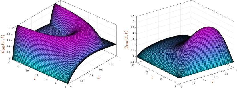
Figure 3: Control and state functions obtained by the proposed method with $n=m=100$ (Example 2).

The obtained control and state functions are in good agreement with the results of Wu and Huang (2018). To report the efficiency and precision of the method, we give in Table 2 the CPU time and the obtained values of the performance index.

Table 2: Consumed CPU time and obtained values of the performance index for various values of $n$ and $m$ (Example 2).

$n$		$m$		CPU Time		$J_{n,m}$
20		20		0.6 s		17.3176450
40		40		3.2 s		17.3055445
60		60		22.7 s		17.3028343
80		80		100.6 s		17.3028684
100		100		311.6 s		17.3028411

Example 3

Now we consider the problem of Example 1 subject to the extra state constraint $y(x,t)\geq y_{\min}(x,t)$, where

$$y_{\min}(x,t):=\sqrt{\max\left\{0,0.1-(x-0.5)^{2}-(t-0.5)^{2}\right\}}.$$

The numerical solution of this problem with indirect methods is troublesome because the derivation of necessary optimality conditions for such optimal control problems with state constraints is difficult. Moreover, the numerical solution of the resulted necessary optimality conditions is complicated. However, extending our direct method to solve such problems is straightforward. We just need to add the following bound constraints to the QP (28):

$$\mathbf{y}_{j}\geq\mathbf{y}_{\min}(\hat{\tau}_{j}),\quad j=1,\dots,m+1,$$

where $\mathbf{y}_{\min}(t):=\big{[}y_{\min}(\hat{\xi}_{1},t),\dots,y_{\min}(\hat{\xi}_{n},t)\big{]}^{\text{T}}$. Imposing the above constraints is simply done by changing the definition of $\mathbf{B}$ and $\mathbf{h}$ in the QP (32) as follows:

$$\mathbf{B}:=-\begin{bmatrix}\mathbf{I}_{n(m+1)}&\big{|}&\mathbf{I}_{nm}\end{bmatrix},\qquad\mathbf{h}:=-\begin{bmatrix}\textbf{vec}\left(\mathbf{Y}_{\min}\right)\\ \hline\cr\textbf{vec}\left(\mathbf{U}_{\min}\right)\end{bmatrix},$$

where

$$\mathbf{Y}_{\min}:=\Big{[}y_{\min}(\hat{\xi}_{i},\hat{\tau}_{j})\Big{]}_{\begin{subarray}{c}i=1,\dots,n\ \ \\ j=1,\dots,m+1\end{subarray}}.$$

By applying our direct method with $n=m=100$, the obtained control and state functions are plotted in Figure 4. Moreover, function $y_{\min}(x,t)$ is plotted beside the state function $y_{100}(x,t)$. It is clear that in this example, contrary to Example 1, the state function is not zero and lies above function $y_{\min}(x,t)$.

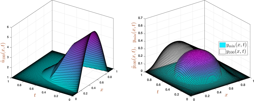
Figure 4: Control and state functions obtained with $n=m=100$ for problem of Example 1 subject to a state constraint $y(x,t)\geq y_{\min}(x,t)$ (Example 3).

Example 4

Consider now problem (1) with

$$r=0.5,\ T=3,\ y(x,0)=\sin(\pi x),\ c(x,t)=1,$$

$$f(x,t)=0,\ z(x,t)=0.5,\ u_{\min}(x,t)=0.$$

In Figure 5, the obtained solutions with $m=n=60$ on this problem, for $\beta=0.1,\,0.5,\,0.9$, are plotted.

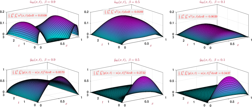
Figure 5: Control and state functions obtained by the presented method with $n=m=60$, for $\beta=0.1,\,0.5,\,0.9$ (Example 4).

Moreover, the values of the first and second terms in the performance index (1d) are reported as well. It is seen, for smaller values of $\beta$, that the obtained state $\tilde{y}_{60}$ is not close to the target function $z(x,t)=\tfrac{1}{2}$. Indeed, when the value of $\beta$ is small, then a large magnitude control function is needed to generate a state function close to $z(x,t)$. In other words, much energy is needed to force $y(x,t)$ to become close to $z(x,t)$. As a result, in these cases, the optimal control is close to its lower bound and the the corresponding state function is not close to the target function.

Example 5

As a final example, let

$$r=0.5,\ T=3,\ y(x,0)=x^{4}(1-x)^{4},u_{\min}(x,t)=1,$$

$$c(x,t)=1,\ z(x,t)=e^{t}x^{4}(1-x)^{4},$$

$$f(x,t)=e^{t}\left[x^{4}(1-x)^{4}-12\left(\bar{f}(x)+\bar{f}(1-x)\right)\right],$$

where

$$\bar{f}(x)=\tfrac{1680{x}^{6+\beta}}{\Gamma\left(7+\beta\right)}-\tfrac{840{x}^{5+\beta}}{\Gamma\left(6+\beta\right)}+\tfrac{180{x}^{4+\beta}}{\Gamma\left(5+\beta\right)}-\tfrac{20{x}^{3+\beta}}{\Gamma\left(4+\beta\right)}+\tfrac{{x}^{2+\beta}}{\Gamma\left(3+\beta\right)}.$$

The exact solution is given by

$$u_{\text{ex}}:=0,\quad y_{\text{ex}}:=e^{t}x^{4}(1-x)^{4},\ \ J_{\text{ex}}=1.5.$$

We applied the presented method on this problem with different values of $\beta$. The obtained errors $E_{n}^{2}(y)$ and $E_{n}(J)$, for various values of $n=m$, are reported in Table 3.

Table 3: Obtained norms of errors for various values of $\beta$ and $n=m$. (Example 5).

		$E_{n}^{2}(y)$						$E_{n}(J)$
$n=m$		$\beta=0.1$	$\beta=0.3$	$\beta=0.5$	$\beta=0.7$	$\beta=0.9$		$\beta=0.1$	$\beta=0.3$	$\beta=0.5$	$\beta=0.7$	$\beta=0.9$
3		1.7e-02	1.4e-02	1.0e-02	6.6e-03	2.7e-03		8.4e-04	5.4e-04	3.0e-04	1.3e-04	2.1e-05
4		4.9e-03	3.8e-03	2.7e-03	1.7e-03	6.7e-04		4.6e-05	2.8e-05	1.5e-05	6.7e-06	1.5e-06
5		5.3e-04	4.5e-04	3.7e-04	2.8e-04	1.5e-04		6.5e-07	4.8e-07	3.3e-07	2.0e-07	6.4e-08
6		1.2e-04	1.2e-04	1.1e-04	9.1e-05	6.0e-05		2.9e-08	2.7e-08	2.3e-08	1.7e-08	8.6e-09
7		8.5e-08	8.9e-08	8.9e-08	8.7e-08	8.2e-08		8.7e-15	1.1e-14	1.3e-14	1.4e-14	1.5e-14
8		7.2e-09	7.3e-09	7.4e-09	8.0e-09	1.1e-08		2.9e-15	4.4e-15	6.2e-15	8.4e-15	1.2e-14
9		9.6e-10	1.3e-09	2.2e-09	4.1e-09	9.4e-09		2.7e-15	4.2e-15	6.2e-15	8.1e-15	9.9e-15
10		8.5e-10	1.3e-09	2.1e-09	4.1e-09	9.5e-09		2.2e-16	9.8e-16	2.7e-15	6.7e-15	8.5e-15

As we see, when $\beta$ is close to 1, then the accuracy is decreased slightly. This fact is predictable. Indeed, if $\beta$ is close to 1, then equation (1a) tends to the advection equation, which is a difficult problem from the numerical point of view. However, we see that our method can obtain a solution with 8 digits of accuracy, even for large values of $\beta$.

6 Conclusions

We proposed a fully direct pseudospectral method to solve the optimal control of a two-sided space-fractional diffusion equation. Thanks to useful properties of the Jacobi polynomials, accurate and stable procedures for deriving the left and right fractional differentiation matrices were presented. In our method, the solution of the problem reduces to the solution of a convex quadratic programming problem. Five examples were solved and results reported. These results show that the fully direct pseudospectral method is efficient and provides accurate results, whereas a small number of collocation points is used and a low CPU time is consumed. Moreover, our third example shows that the method here introduced can be also applied with success to difficult optimal control problems with inequality constraints on the state function.

Obtaining some theoretical estimates for the approximation errors would be desirable. This work is currently in progress.

Torres has been partially supported by FCT (The Portuguese National Science Foundation) through the R&D unit CIDMA, project UID/MAT/04106/2013. Bozorgnia was supported by FCT fellowship SFRH/BPD/33962/2009.

The authors are very grateful to three anonymous referees for carefully reading their manuscript and for several comments and suggestions which helped them to improve the paper.

References

- (1)
- Agarwal et al. (2018) Agarwal RP, Baleanu D, Nieto JJ, Torres DFM and Zhou Y (2018) A survey on fuzzy fractional differential and optimal control nonlocal evolution equations. Journal of Computational and Applied Mathematics 339: 3–29. arXiv:1709.07766
- Bai et al. (2018) Bai Y, Baleanu D and Wu GC (2018) Existence and discrete approximation for optimization problems governed by fractional differential equations. Communications in Nonlinear Science and Numerical Simulation 59: 338–348.
- Baltensperger and Trummer (2003) Baltensperger R and Trummer MR (2003) Spectral differencing with a twist. SIAM Journal on Scientific Computing 24(5): 1465–1487.
- Behroozifar and Habibi (2018) Behroozifar M and Habibi N (2018) A numerical approach for solving a class of fractional optimal control problems via operational matrix Bernoulli polynomials. JVC/Journal of Vibration and Control 24(12): 2494–2511.
- Benson et al. (2006) Benson DA, Huntington GT, Thorvaldsen TP and Rao AV (2006) Direct trajectory optimization and costate estimation via an orthogonal collocation method. Journal of Guidance, Control, and Dynamics 29(6): 1435–1440.
- Bhrawy and Zaky (2015) Bhrawy A and Zaky M (2015) A method based on the Jacobi tau approximation for solving multi-term time–space fractional partial differential equations. Journal of Computational Physics 281: 876–895.
- Bhrawy and Zaky (2016) Bhrawy A and Zaky M (2016) Shifted fractional-order Jacobi orthogonal functions: Application to a system of fractional differential equations. Applied Mathematical Modelling 40(2): 832–845.
- Chen et al. (2018) Chen S, Liu F, Turner I and Anh V (2018) A fast numerical method for two-dimensional Riesz space fractional diffusion equations on a convex bounded region. Applied Numerical Mathematics 134: 66–80. 10.1016/j.apnum.2018.07.007.
- Darehmiraki et al. (2018) Darehmiraki M, Farahi M and Effati S (2018) Solution for fractional distributed optimal control problem by hybrid meshless method. JVC/Journal of Vibration and Control 24(11): 2149–2164.
- Dehghan et al. (2016) Dehghan M, Hamedi EA and Khosravian-Arab H (2016) A numerical scheme for the solution of a class of fractional variational and optimal control problems using the modified jacobi polynomials. JVC/Journal of Vibration and Control 22(6): 1547–1559.
- Doha et al. (2014) Doha E, Bhrawy A, Baleanu D and Ezz-Eldien S (2014) The operational matrix formulation of the Jacobi tau approximation for space fractional diffusion equation. Advances in Difference Equations 2014(1): 1–14.
- Dorville et al. (2011) Dorville R, Mophou GM and Valmorin VS (2011) Optimal control of a nonhomogeneous Dirichlet boundary fractional diffusion equation. Computers & Mathematics with Applications 62(3): 1472–1481.
- Du et al. (2016) Du N, Wang H and Liu W (2016) A fast gradient projection method for a constrained fractional optimal control. Journal of Scientific Computing 68(1): 1–20.
- Elnagar et al. (1995) Elnagar G, Kazemi M and Razzaghi M (1995) The pseudospectral Legendre method for discretizing optimal control problems. IEEE Transactions on Automatic Control 40(10): 1793–1796.
- Esmaeili and Shamsi (2011) Esmaeili S and Shamsi M (2011) A pseudo-spectral scheme for the approximate solution of a family of fractional differential equations. Communications in Nonlinear Science and Numerical Simulation 16(9): 3646–3654.
- Esmaeili et al. (2011) Esmaeili S, Shamsi M and Luchko Y (2011) Numerical solution of fractional differential equations with a collocation method based on Müntz polynomials. Computers & Mathematics with Applications 62(3): 918–929.
- Ezz-Eldien et al. (2017) Ezz-Eldien S, Doha E, Baleanu D and Bhrawy A (2017) A numerical approach based on Legendre orthonormal polynomials for numerical solutions of fractional optimal control problems. JVC/Journal of Vibration and Control 23(1): 16–30.
- Fahroo and Ross (2001) Fahroo F and Ross IM (2001) Costate estimation by a Legendre pseudospectral method. Journal of Guidance, Control, and Dynamics 24(2): 270–277.
- Feng et al. (2018) Feng L, Liu F, Turner I, Yang Q and Zhuang P (2018) Unstructured mesh finite difference/finite element method for the 2D time-space Riesz fractional diffusion equation on irregular convex domains. Applied Mathematical Modelling 59: 441–463. 10.1016/j.apm.2018.01.044.
- Foroozandeh et al. (2017) Foroozandeh Z, Shamsi M, Azhmyakov V and Shafiee M (2017) A modified pseudospectral method for solving trajectory optimization problems with singular arc. Mathematical Methods in the Applied Sciences 40(5): 1783–1793.
- Foroozandeh et al. (2018) Foroozandeh Z, Shamsi M and d R de Pinho M (2018) A mixed-binary non-linear programming approach for the numerical solution of a family of singular optimal control problems. International Journal of Control 10.1080/00207179.2017.1399216.
- Garg (2011) Garg D (2011) Advances in global pseudospectral methods for optimal control. PhD Thesis, University of Florida.
- Garg et al. (2010) Garg D, Patterson M, Hager WW, Rao AV, Benson DA and Huntington GT (2010) A unified framework for the numerical solution of optimal control problems using pseudospectral methods. Automatica 46(11): 1843–1851.
- Gautschi (1996) Gautschi W (1996) Orthogonal Polynomials: applications and computation. in A. Iserles (Ed.), Acta Numerica, Cambridge Univ. Press.
- Khaksar-e Oshagh and Shamsi (2017) Khaksar-e Oshagh M and Shamsi M (2017) Direct pseudo-spectral method for optimal control of obstacle problem – an optimal control problem governed by elliptic variational inequality. Mathematical Methods in the Applied Sciences 40(13): 4993–5004.
- Laub (2005) Laub A (2005) Matrix Analysis for Scientists and Engineers. Society for Industrial and Applied Mathematics.
- Li and Zhou (2018) Li S and Zhou Z (2018) Legendre pseudo-spectral method for optimal control problem governed by a time-fractional diffusion equation. International Journal of Computer Mathematics 95(6-7): 1308–1325. 10.1080/00207160.2017.1417591.
- Malinowska and Torres (2012) Malinowska AB and Torres DFM (2012) Introduction to the fractional calculus of variations. Imperial College Press, London.
- Mashayekhi and Razzaghi (2018) Mashayekhi S and Razzaghi M (2018) An approximate method for solving fractional optimal control problems by hybrid functions. JVC/Journal of Vibration and Control 24(9): 1621–1631.
- Meerschaert and Tadjeran (2006) Meerschaert MM and Tadjeran C (2006) Finite difference approximations for two-sided space-fractional partial differential equations. Applied Numerical Mathematics 56(1): 80–90.
- Mohammadzadeh et al. (2018) Mohammadzadeh E, Pariz N, Hosseini Sani S and Jajarmi A (2018) An efficient numerical method for the optimal control of fractional-order dynamic systems. JVC/Journal of Vibration and Control 10.1177/1077546317751755.
- Mophou and N’Guérékata (2011) Mophou G and N’Guérékata GM (2011) Optimal control of a fractional diffusion equation with state constraints. Computers & Mathematics with Applications 62(3): 1413–1426.
- Mophou (2011) Mophou GM (2011) Optimal control of fractional diffusion equation. Computers & Mathematics with Applications 61(1): 68–78.
- Pooseh et al. (2013) Pooseh S, Almeida R and Torres DFM (2013) Discrete direct methods in the fractional calculus of variations. Computers & Mathematics with Applications 66(5): 668–676. arXiv:1205.4843
- Salati et al. (2019) Salati AB, Shamsi M and Torres DFM (2019) Direct transcription methods based on fractional integral approximation formulas for solving nonlinear fractional optimal control problems. Communications in Nonlinear Science and Numerical Simulation 67: 334–350. 10.1016/j.cnsns.2018.05.011. arXiv:1805.06537
- Tang et al. (2017) Tang X, Shi Y and Wang LL (2017) A new framework for solving fractional optimal control problems using fractional pseudospectral methods. Automatica 78: 333–340.
- Wächter and Biegler (2006) Wächter A and Biegler LT (2006) On the implementation of an interior-point filter line-search algorithm for large-scale nonlinear programming. Mathematical Programming 106(1, Ser. A): 25–57.
- Wu et al. (2015) Wu GC, Baleanu D, Deng ZG and Zeng SD (2015) Lattice fractional diffusion equation in terms of a Riesz-Caputo difference. Physica A: Statistical Mechanics and its Applications 438: 335–339. 10.1016/j.physa.2015.06.024.
- Wu et al. (2017) Wu GC, Baleanu D, Xie HP and Zeng SD (2017) Lattice fractional diffusion equation of random order. Mathematical Methods in the Applied Sciences 40(17): 6054–6060. 10.1002/mma.3644.
- Wu and Huang (2018) Wu SL and Huang TZ (2018) A fast second-order parareal solver for fractional optimal control problems. Journal of Vibration and Control 24(15): 3418–3433. 10.1177/1077546317705557.
- Yamamoto (2018) Yamamoto M (2018) Weak solutions to non-homogeneous boundary value problems for time-fractional diffusion equations. Journal of Mathematical Analysis and Applications 460(1): 365–381.
- Yang and Machado (2017) Yang XJ and Machado J (2017) A new fractional operator of variable order: Application in the description of anomalous diffusion. Physica A: Statistical Mechanics and its Applications 481: 276–283.
- Yang et al. (2017a) Yang XJ, Machado J and Baleanu D (2017a) Anomalous diffusion models with general fractional derivatives within the kernels of the extended Mittag-Leffler type functions. Romanian Reports in Physics 69(4).
- Yang et al. (2016) Yang XJ, Machado J, Baleanu D and Gao F (2016) A new numerical technique for local fractional diffusion equation in fractal heat transfer. Journal of Nonlinear Science and Applications 9(10): 5621–5628.
- Yang et al. (2017b) Yang XJ, Srivastava H, Torres D and Debbouche A (2017b) General fractional-order anomalous diffusion with non-singular power-law kernel. Thermal Science 21: S1–S9.
- Yang et al. (2017c) Yang Z, Yuan Z, Nie Y, Wang J, Zhu X and Liu F (2017c) Finite element method for nonlinear Riesz space fractional diffusion equations on irregular domains. Journal of Computational Physics 330: 863–883. 10.1016/j.jcp.2016.10.053.
- Zaky (2018) Zaky M (2018) A Legendre collocation method for distributed-order fractional optimal control problems. Nonlinear Dynamics 91(4): 2667–2681.
- Zaky et al. (2018) Zaky M, Doha E and Machado JT (2018) A spectral framework for fractional variational problems based on fractional Jacobi functions. Applied Numerical Mathematics 132: 51–72. 10.1016/j.apnum.2018.05.009.
- Zaky et al. (2016) Zaky M, Ezz-Eldien S, Doha E, Machado J and Bhrawy A (2016) An efficient operational matrix technique for multidimensional variable-order time fractional diffusion equations. Journal of Computational and Nonlinear Dynamics 11(6).
- Zaky and Machado (2017) Zaky MA and Machado JAT (2017) On the formulation and numerical simulation of distributed-order fractional optimal control problems. Communications in Nonlinear Science and Numerical Simulation 52: 177–189.
- Zayernouri and Karniadakis (2013) Zayernouri M and Karniadakis GE (2013) Fractional Sturm-Liouville eigen-problems: Theory and numerical approximation. Journal of Computational Physics 252: 495–517.