A cholera mathematical model with vaccination and the biggest outbreak
of world’s history

Abstract

We propose and analyse a mathematical model for cholera considering vaccination. We show that the model is epidemiologically and mathematically well posed and prove the existence and uniqueness of disease-free and endemic equilibrium points. The basic reproduction number is determined and the local asymptotic stability of equilibria is studied. The biggest cholera outbreak of world’s history began on 27${}^{\text{th}}$ April 2017, in Yemen. Between 27${}^{\text{th}}$ April 2017 and 15${}^{\text{th}}$ April 2018 there were 2275 deaths due to this epidemic. A vaccination campaign began on 6${}^{\text{th}}$ May 2018 and ended on 15${}^{\text{th}}$ May 2018. We show that our model is able to describe well this outbreak. Moreover, we prove that the number of infected individuals would have been much lower provided the vaccination campaign had begun earlier.

1 Introduction

Cholera is an acute diarrhoeal illness caused by infection of the intestine with bacterium vibrio cholerae, which lives in an aquatic organism [16]. The ingestion of contaminated water can cause cholera outbreaks, as John Snow proved in 1854 [24]. This is a possibility of transmission of the disease, but others do exist. For example, susceptible individuals can become infected if they become in contact with contaminated people. When individuals are at an increased risk of infection, then they can transmit the disease to those who live with them, by reflecting food preparation or using water storage containers [24]. An individual can be infected with or without symptoms and some of these can be watery diarrhea, vomiting and leg cramps. If contaminated individuals do not get treatment, then they become dehydrated, suffering acidosis and circulatory collapse. This situation can lead to death within 12 to 24 hours [18, 24]. Some studies and experiments suggest that a recovered individual can be immune to the disease during a period of 3 to 10 years. Nevertheless, recent researches conclude that immunity can be lost after a period of weeks to months [19, 24].

Since 1979, several mathematical models for the transmission of cholera have been proposed: see, e.g., [2, 3, 8, 9, 11, 14, 16, 17, 18, 19, 22, 24] and references cited therein. In [19], the authors propose a SIR (Susceptible–Infectious–Recovered) type model and consider two classes of bacterial concentrations (hyperinfectious and less-infectious) and two classes of infectious individuals (asymptomatic and symptomatic). In [24], another SIR-type model is proposed that incorporates hyperinfectivity (where infectivity varies with time since the pathogen was shed) and temporary immunity, using distributed delays. The authors of [18] incorporate in a SIR-type model public health educational campaigns, vaccination, quarantine and treatment, as control strategies in order to curtail the disease.

Between 2007 and 2018, several cholera outbreaks occurred, namely in Angola, Haiti, Zimbabwe and Yemen [1, 24, 31]. Mathematical models have been developed and studied in order to understand the transmission dynamics of cholera epidemics, mostly focusing on the epidemic that occurred in Haiti, 2010–2011 [1]. In [16], a SIQR (Susceptible–Infectious–Quarantined–Recovered) type model, which also considers a class for bacterial concentration, is analysed, being shown that it fits well the cholera outbreak in the Department of Artibonite – Haiti, from 1${}^{\text{st}}$ November 2010 until 1${}^{\text{st}}$ May 2011. Furthermore, an optimal control problem is formulated and solved, where the optimal control function represents the fraction of infected individuals that are submitted to treatment through quarantine [16]. Many studies have been developed with the purpose to find and evaluate measures to contain the cholera spread. Nevertheless, it was not possible yet to obtain solutions in real time that can stop the cholera epidemics [1].

Recently, the biggest outbreak of cholera in the history of the world has occurred in Yemen [26]. The epidemic began in October 2016 and in February-March 2017 was in decline. However, on 27${}^{\text{th}}$ April 2017 the epidemic returned. This happened ten days after Sana’a’s sewer system had stopped working. Problems in infrastructures, health, water and sanitation systems in Yemen, allowed the fast spread of the disease [28]. Between 27${}^{\text{th}}$ April 2017 and 15${}^{\text{th}}$ April 2018 there were 1 090 280 suspected cases reported and 2 275 deaths due to cholera [32]. In [20], Nishiura et al. study mathematically this outbreak, trying to forecast the cholera epidemic in Yemen, explicitly addressing the reporting delay and ascertainment bias. A vaccine for cholera is currently available, but poor sanitation and the lack of access to vaccines promote the spread of the disease [1].

Following World Health Organization (WHO) recommendations, the first-ever oral vaccination campaign against cholera had been launched on 6${}^{\text{th}}$ May 2018 in Yemen, but it was concluded on 15${}^{\text{th}}$ May 2018 [30], due to the lack of national governmental authorization to do the vaccination [23]. Aid workers say that one reason of the delayed of the campaign vaccination is due to some senior Houthi officials who objected to vaccination. This campaign coincided with the rainy season and some health workers fear that this could spread the disease [23]. This campaign just covered four districts in Aden, which were at a high risk of fast spread of the disease, and just 350 000 individuals (including pregnant women) were vaccinated [23, 26]. It is important to note that the vaccinated individuals represent, approximately, 1.21% of the total population, since the total population of Yemen, in 2018, is 28 915 284 [34]. Lorenzo Pizzoli, WHO’s cholera expert, said that the campaign hoped to cover at least four million people in areas at risk (corresponding, approximately, to 14% of total population) and Michael Ryan, WHO’s Assistant Director-General, revealed that they were negotiating with Yemen health authorities in order to vaccinate people from all high risks zones [23]. The International Coordinating Group on Vaccine Provision had planned one million cholera vaccines for Yemen in July 2017, but WHO and Yemen local authorities decided to postpone it and the doses were diverted to South Sudan. WHO and GAVI, the Vaccine Alliance, affirmed that the largest cholera vaccination is now being carried out in five countries (Kenya, Malawi, South Sudan, Uganda and Zambia). It is expected that this campaign targets more than two million people across Africa [23].

In this paper, we propose a SITRV (Susceptible–Infectious–Treated–Recovered–Vaccinated) type model, which includes a class of bacterial concentration. In Section 2, we formulate and explain the mathematical model. Then, in Section 3, we show that the model is mathematically well posed and it has biological meaning. We prove the existence and uniqueness of the disease-free and endemic equilibrium points and compute the basic reproduction number. The sensitivity of the basic reproduction number with respect to all parameters of the model is analysed in Subsection 3.3 and the stability analysis of equilibria is carried out in Subsection 3.4. In Section 4, we show that the model fits well the cholera outbreak in Yemen, between 27${}^{\text{th}}$ April 2017 and 15${}^{\text{th}}$ April 2018. Through numerical simulations, we illustrate the impact of vaccination of susceptible individuals in Yemen. We end with Section 5, by deriving some conclusions about the importance of vaccination campaigns on the control and eradication of a cholera outbreak.

We trust that our work is of great significance, because it provides a mathematical model for cholera that is deeply studied and allows to obtain important conclusions about the relevance of vaccination campaigns in cholera outbreaks. We show that, if it had existed a vaccination campaign from the beginning of the outbreak in Yemen, then the epidemic would have been extinguished. Actually, we believe that the absence of this type of prevention measures in Yemen, was one of the responsible for provoking the biggest cholera outbreak in world’s history [26], killing 2275 individuals until 15${}^{\text{th}}$ April 2018.

2 Model formulation

We modify the model studied in [16], adding a vaccination class and considering different kinds of cholera’s treatment. The model is a SITRV (Susceptible–Infectious–Treated–Recovered–Vaccinated) type model and considers a class of bacterial concentration for the dynamics of cholera. The total human population $N(t)$ is divided into five classes: susceptible $S(t)$, infectious with symptoms $I(t)$, in treatment $T(t)$, recovered $R(t)$ and vaccinated $V(t)$ at time $t$, for $t\geq 0$. Furthermore, we consider a class $B(t)$ that reflects the bacterial concentration at time $t$. We assume that there is a positive recruitment rate $\Lambda$ into the susceptible class $S(t)$ and a positive natural death rate $\mu$, for all time $t$ under study. Susceptible individuals can be vaccinated at rate $\varphi\geq 0$ and become infected with cholera at rate $\displaystyle\frac{\beta B(t)}{\kappa+B(t)}\geq 0$, which is dependent on time $t$. Note that $\beta>0$ is the ingestion rate of the bacterium through contaminated sources, $\kappa>0$ is the half saturation constant of the bacterial population, and $\displaystyle\frac{B(t)}{\kappa+B(t)}$ measures the possibility of an infected individual to have the disease with symptoms, given a contact with contaminated sources [18]. Any recovered and vaccinated individual can lose the immunity at rate $\omega_{1}\geq 0$ and $\omega_{2}\geq 0$, respectively, becoming susceptible again. Different types of treatment for cholera infected individuals are considered based on [29]. The infected individuals can get a proper treatment, at rate $\delta\geq 0$, and the individuals in treatment can recover at rate $\varepsilon\geq 0$. The disease-related death rates associated with the individuals that are infected and in treatment are $\alpha_{1}\geq 0$ and $\alpha_{2}\geq 0$, respectively. Each infected individual contributes to the increase of the bacterial concentration at rate $\eta>0$. On the other hand, the bacterial concentration can decrease at mortality rate $d>0$. These assumptions are translated into the following mathematical model:

$$\begin{cases}S^{\prime}(t)=\Lambda-\displaystyle\frac{\beta B(t)}{\kappa+B(t)}S(t)+\omega_{1}R(t)+\omega_{2}V(t)-(\varphi+\mu)S(t),\\ I^{\prime}(t)=\displaystyle\frac{\beta B(t)}{\kappa+B(t)}S(t)-\left(\delta+\alpha_{1}+\mu\right)I(t),\\ T^{\prime}(t)=\delta I(t)-(\varepsilon+\alpha_{2}+\mu)T(t),\\ R^{\prime}(t)=\varepsilon T(t)-(\omega_{1}+\mu)R(t),\\ V^{\prime}(t)=\varphi S(t)-(\omega_{2}+\mu)V(t),\\ B^{\prime}(t)=\eta I(t)-dB(t).\end{cases}$$ (2.1)

3 Model analysis

Throughout the paper, we assume that the initial conditions of system (2.1) are non-negative:

$$S(0)=S_{0}\geq 0,\ I(0)=I_{0}\geq 0,\ T(0)=T_{0}\geq 0,\ R(0)=R_{0}\geq 0,\ V(0)=V_{0}\geq 0,\ B(0)=B_{0}\geq 0.$$ (3.1)

3.1 Positivity and boundedness of solutions

Our first lemma shows that the considered model (2.1)–(3.1) is biologically meaningful.

Lemma 1.

The solutions $(S(t),I(t),T(t),R(t),V(t),B(t))$ of system (2.1) are non-negative for all $t\geq 0$ with non-negative initial conditions (3.1) in $(\mathbb{R}_{0}^{+})^{6}$.

Proof.

We have

$$\begin{cases}\frac{dS(t)}{dt}\Bigg{|}_{\xi(S)}&=\Lambda+\omega_{1}R(t)+\omega_{2}V(t)>0\,,\\ \frac{dI(t)}{dt}\Bigg{|}_{\xi(I)}&=\frac{\beta B(t)}{\kappa+B(t)}S(t)\geq 0\,,\\ \frac{dT(t)}{dt}\Bigg{|}_{\xi(Q)}&=\delta I(t)\geq 0\,,\\ \frac{dR(t)}{dt}\Bigg{|}_{\xi(R)}&=\varepsilon T(t)\geq 0\,,\\ \frac{dV(t)}{dt}\Bigg{|}_{\xi(V)}&=\varphi S(t)\geq 0\,,\\ \frac{dB(t)}{dt}\Bigg{|}_{\xi(B)}&=\eta I(t)\geq 0\,,\end{cases}$$

where $\xi(\upsilon)=\left\{\upsilon(t)=0\text{ and }S,I,T,R,V,B\in C(\mathbb{R}_{0}^{+},\mathbb{R}_{0}^{+})\right\}$ and $\upsilon\in\{S,I,T,R,V,B\}$. Therefore, due to Lemma 2 in [33], any solution of system (2.1) is such that $(S(t),I(t),T(t),R(t),V(t),B(t))\in(\mathbb{R}_{0}^{+})^{6}$ for all $t\geq 0$. ∎

Lemma 2 shows that it is enough to consider the dynamics of the flow generated by (2.1)–(3.1) in a certain region $\Omega_{V}$.

Lemma 2.

Let

$$\Omega_{H}=\left\{(S,I,T,R,V)\in\left(\mathbb{R}_{0}^{+}\right)^{5}\,|\,0\leq S(t)+I(t)+T(t)+R(t)+V(t)\leq\frac{\Lambda}{\mu}\right\}$$ (3.2)

and

$$\Omega_{B}=\left\{B\in\mathbb{R}_{0}^{+}\,|\,0\leq B(t)\leq\frac{\Lambda\eta}{\mu d}\right\}.$$ (3.3)

Define

$$\Omega_{V}=\Omega_{H}\times\Omega_{B}.$$ (3.4)

If $N(0)\leq\displaystyle\frac{\Lambda}{\mu}$ and $B(0)\leq\displaystyle\frac{\Lambda\eta}{\mu d}$, then the region $\Omega_{V}$ is positively invariant for model (2.1) with non-negative initial conditions (3.1) in $(\mathbb{R}_{0}^{+})^{6}$.

Proof.

Let us split system (2.1) into two parts: the human population, i.e., $S(t)$, $I(t)$, $T(t)$, $R(t)$ and $V(t)$, and the pathogen population, i.e., $B(t)$. Adding the first five equations of system (2.1) gives

$$N^{\prime}(t)=S^{\prime}(t)+I^{\prime}(t)+T^{\prime}(t)+R^{\prime}(t)+V^{\prime}(t)=\Lambda-\mu N(t)-\alpha_{1}I(t)-\alpha_{2}T(t)\leq\Lambda-\mu N(t)\,.$$

Assuming that $N(0)\leq\frac{\Lambda}{\mu}$, we conclude that $N(t)\leq\frac{\Lambda}{\mu}$. For this reason, (3.2) defines the biologically feasible region for the human population. As it is proved in [16], the region (3.3) defines the biologically feasible region for the pathogen population. From (3.2) and (3.3), we know that $N(t)$ and $B(t)$ are bounded for all $t\geq 0$. Therefore, every solution of system (2.1) with initial conditions in $\Omega_{V}$ remains in $\Omega_{V}$ for all $t\geq 0$. In other words, in region $\Omega_{V}$ defined by (3.4), our model is epidemiologically and mathematically well posed in the sense of [10]. ∎

3.2 Equilibrium points and basic reproduction number

From now on, let us consider that $a_{0}=\varphi+\mu$, $a_{1}=\delta+\alpha_{1}+\mu$, $a_{2}=\varepsilon+\alpha_{2}+\mu$, $a_{3}=\omega_{1}+\mu$ and $a_{4}=\omega_{2}+\mu$. The disease-free equilibrium (DFE) of model (2.1) is given by

$$E^{0}=\left(S^{0},I^{0},T^{0},R^{0},V^{0},B^{0}\right)=\left(\frac{\Lambda a_{4}}{a_{0}a_{4}-\varphi\omega_{2}},0,0,0,\frac{\Lambda\varphi}{a_{0}a_{4}-\varphi\omega_{2}},0\right).$$ (3.5)

Remark 1.

Note that, because $\mu>0$, one has $a_{0}a_{4}-\varphi\omega_{2}=(\varphi+\mu)(\omega_{2}+\mu)-\varphi\omega_{2}>0$.

Next, following the approach of [18, 27], we compute the basic reproduction number $R_{0}$.

Proposition 3 (Basic reproduction number of (2.1)).

The basic reproduction number of model (2.1) is given by

$$R_{0}=\frac{\beta\Lambda\eta a_{4}}{(a_{0}a_{4}-\varphi\omega_{2})\kappa da_{1}}.$$ (3.6)

Proof.

Consider that $\mathcal{F}_{i}(t)$ is the rate of appearance of new infections in the compartment associated with index $i$, $\mathcal{V}_{i}^{+}(t)$ is the rate of transfer of “individuals” into the compartment associated with index $i$ by all other means and $\mathcal{V}_{i}^{-}(t)$ is the rate of transfer of “individuals” out of compartment associated with index $i$. In this way, the matrices $\mathcal{F}(t)$, $\mathcal{V}^{+}(t)$ and $\mathcal{V}^{-}(t)$, associated with model (2.1), are given by

$$\mathcal{F}(t)=\left[\begin{matrix}0\\ \displaystyle\frac{\beta B(t)S(t)}{\kappa+B(t)}\\ 0\\ 0\\ 0\\ 0\end{matrix}\right],\quad\mathcal{V}^{+}(t)=\left[\begin{matrix}\Lambda+\omega_{1}R(t)+\omega_{2}V(t)\\ 0\\ \delta I(t)\\ \varepsilon T(t)\\ \varphi S(t)\\ \eta I(t)\end{matrix}\right]\quad\text{ and }\quad\mathcal{V}^{-}(t)=\left[\begin{matrix}\displaystyle\frac{\beta B(t)S(t)}{\kappa+B(t)}+a_{0}S(t)\\ a_{1}I(t)\\ a_{2}T(t)\\ a_{3}R(t)\\ a_{4}V(t)\\ dB(t)\end{matrix}\right].$$

Therefore, by considering $\mathcal{V}(t)=\mathcal{V}^{-}(t)-\mathcal{V}^{+}(t)$, we have that

$$\left[\begin{matrix}S^{\prime}(t)&I^{\prime}(t)&T^{\prime}(t)&R^{\prime}(t)&V^{\prime}(t)&B^{\prime}(t)\end{matrix}\right]^{T}=\mathcal{F}(t)-\mathcal{V}(t).$$

The Jacobian matrices of $\mathcal{F}(t)$ and of $\mathcal{V}(t)$ are, respectively, given by

$$F=\left[\begin{matrix}0&0&0&0&0&0\\ \displaystyle\frac{\beta B(t)}{\kappa+B(t)}&0&0&0&0&\displaystyle\frac{\beta\kappa S(t)}{(\kappa+B(t))^{2}}\\ 0&0&0&0&0&0\\ 0&0&0&0&0&0\\ 0&0&0&0&0&0\\ 0&0&0&0&0&0\end{matrix}\right]\text{ and }V=\left[\begin{matrix}\displaystyle\frac{\beta B(t)}{\kappa+B(t)}+a_{0}&0&0&-\omega_{1}&-\omega_{2}&\displaystyle\frac{\beta\kappa S(t)}{(\kappa+B(t))^{2}}\\ 0&a_{1}&0&0&0&0\\ 0&-\delta&a_{2}&0&0&0\\ 0&0&-\varepsilon&a_{3}&0&0\\ -\varphi&0&0&0&a_{4}&0\\ 0&-\eta&0&0&0&d\\ \end{matrix}\right].$$

In the disease-free equilibrium $E^{0}$ defined by (3.5), we obtain the matrices $F_{0}$ and $V_{0}$ given by

$$F_{0}=\left[\begin{matrix}0&0&0&0&0&0\\ 0&0&0&0&0&\displaystyle\frac{\beta\Lambda a_{4}}{(a_{0}a_{4}-\varphi\omega_{2})\kappa}\\ 0&0&0&0&0&0\\ 0&0&0&0&0&0\\ 0&0&0&0&0&0\\ 0&0&0&0&0&0\end{matrix}\right]\quad\text{ and }\quad V_{0}=\left[\begin{matrix}a_{0}&0&0&-\omega_{1}&-\omega_{2}&\displaystyle\frac{\beta\Lambda a_{4}}{(a_{0}a_{4}-\varphi\omega_{2})\kappa}\\ 0&a_{1}&0&0&0&0\\ 0&-\delta&a_{2}&0&0&0\\ 0&0&-\varepsilon&a_{3}&0&0\\ -\varphi&0&0&0&a_{4}&0\\ 0&-\eta&0&0&0&d\\ \end{matrix}\right].$$

The basic reproduction number of model (2.1) is then given by

$$R_{0}=\rho(F_{0}V_{0}^{-1})=\frac{\beta\Lambda\eta a_{4}}{(a_{0}a_{4}-\varphi\omega_{2})\kappa da_{1}},$$

found with the help of the computer algebra system Maple. This concludes the proof. ∎

Now we prove the existence of an endemic equilibrium when $R_{0}$ given by (3.6) is greater than one.

Proposition 4 (Endemic equilibrium).

If the basic reproduction number (3.6) is such that $R_{0}>1$, then the model (2.1) has an endemic equilibrium given by

$$E^{*}=(S^{*},I^{*},T^{*},R^{*},V^{*},B^{*}),$$ (3.7)

where

$$\begin{cases}S^{*}=\displaystyle\frac{a_{1}a_{4}\{\kappa d(a_{1}a_{2}a_{3}-\delta\varepsilon\omega_{1})+\Lambda\eta a_{2}a_{3}\}}{\eta\tilde{D}}\\[8.5359pt] I^{*}=\displaystyle\frac{a_{2}a_{3}\{\beta\Lambda\eta a_{4}-(a_{0}a_{4}-\varphi\omega_{2})\kappa da_{1}\}}{\eta\tilde{D}}\\[8.5359pt] T^{*}=\displaystyle\frac{a_{3}\delta\{\beta\Lambda\eta a_{4}-(a_{0}a_{4}-\varphi\omega_{2})\kappa da_{1}\}}{\eta\tilde{D}}\\[8.5359pt] R^{*}=\displaystyle\frac{\delta\epsilon\{\beta\Lambda\eta a_{4}-(a_{0}a_{4}-\varphi\omega_{2})\kappa da_{1}\}}{\eta\tilde{D}}\\[8.5359pt] V^{*}=\displaystyle\frac{a_{1}\varphi\{\kappa d(a_{1}a_{2}a_{3}-\delta\varepsilon\omega_{1})+\Lambda\eta a_{2}a_{3}\}}{\eta\tilde{D}}\\[8.5359pt] B^{*}=\displaystyle\frac{a_{2}a_{3}\{\beta\Lambda\eta a_{4}-(a_{0}a_{4}-\varphi\omega_{2})\kappa da_{1}\}}{d\tilde{D}}\end{cases}$$

and $\tilde{D}=\left\{a_{1}a_{2}a_{3}(a_{0}a_{4}-\varphi\omega_{2})+\beta a_{4}(a_{1}a_{2}a_{3}-\delta\varepsilon\omega_{1})\right\}$.

Proof.

We note that

1. $a_{1}=\delta+\alpha_{1}+\mu>0$, because $\delta$, $\alpha_{1}\geq 0$ and $\mu>0$;

2. $a_{2}=\varepsilon+\alpha_{2}+\mu>0$, because $\varepsilon$, $\alpha_{2}\geq 0$ and $\mu>0$;

3. $a_{3}=\omega_{1}+\mu>0$, because $\omega_{1}\geq 0$ and $\mu>0$;

4. $\beta$, $\kappa$, $d>0$ and $\varphi\geq 0$;

5. $a_{0}a_{4}-\varphi\omega_{2}>0$ (see Remark 1);

6. $a_{1}a_{2}a_{3}-\delta\varepsilon\omega_{1}=(\delta+\alpha_{1}+\mu)(\varepsilon+\alpha_{2}+\mu)(\omega_{1}+\mu)-\delta\varepsilon\omega_{1}>0$, because $\alpha_{1}$, $\alpha_{2}\geq 0$ and $\mu>0$;

7. $\Lambda\eta a_{2}a_{3}>0$, because $\Lambda$, $\eta$, $a_{2}$, $a_{3}>0$.

With the above inequalities, we conclude that $\tilde{D}>0$ and, consequently, that $S^{*}>0$ and $V^{*}\geq 0$. The basic reproduction number is given by $\displaystyle\frac{\beta\Lambda\eta a_{4}}{(a_{0}a_{4}-\varphi\omega_{2})\kappa da_{1}}$. Thus, it follows that

$$\ \beta\Lambda\eta a_{4}=R_{0}(a_{0}a_{4}-\varphi\omega_{2})\kappa da_{1}$$

$$\Leftrightarrow \ \beta\Lambda\eta a_{4}-(a_{0}a_{4}-\varphi\omega_{2})\kappa da_{1}=R_{0}(a_{0}a_{4}-\varphi\omega_{2})\kappa da_{1}-(a_{0}a_{4}-\varphi\omega_{2})\kappa da_{1}$$

$$\Leftrightarrow \ \beta\Lambda\eta a_{4}-(a_{0}a_{4}-\varphi\omega_{2})\kappa da_{1}=(a_{0}a_{4}-\varphi\omega_{2})\kappa da_{1}(R_{0}-1).$$

Therefore, we have that

$$\begin{cases}I^{*}=\displaystyle\frac{a_{1}a_{2}a_{3}\kappa d(a_{0}a_{4}-\varphi\omega_{2})(R_{0}-1)}{\eta\tilde{D}}\\[8.5359pt] T^{*}=\displaystyle\frac{a_{1}a_{3}\kappa d\delta(a_{0}a_{4}-\varphi\omega_{2})(R_{0}-1)}{\eta\tilde{D}}\\[8.5359pt] R^{*}=\displaystyle\frac{a_{1}\kappa d\delta\varepsilon(a_{0}a_{4}-\varphi\omega_{2})(R_{0}-1)}{\eta\tilde{D}}\\[8.5359pt] B^{*}=\displaystyle\frac{a_{1}a_{2}a_{3}\kappa(a_{0}a_{4}-\varphi\omega_{2})(R_{0}-1)}{\tilde{D}}.\end{cases}$$

In order to obtain an endemic equilibrium, we have to ensure that $I^{*}$, $B^{*}>0$. Thus, we obtain $I^{*}$, $B^{*}>0$ if and only if $R_{0}-1>0\Leftrightarrow R_{0}>1$. In this case ($R_{0}>1$), we also have that $T^{*}$, $R^{*}\geq 0$. ∎

3.3 Sensitivity of the basic reproduction number

In this section, we are going to study the sensitivity of $R_{0}$ with respect to all parameters $p$ of model (2.1), computing the respective normalized forward sensitive indexes $\Upsilon^{R_{0}}_{p}$ given in Definition 1. They are presented in Table 1.

Definition 1 (See [6, 15, 25]).

The normalized forward sensitivity index of a variable $z$ that depends differentiably on a parameter $p$ is defined by

$$\Upsilon^{z}_{p}=\frac{\partial z}{\partial p}\times\frac{p}{|z|}.$$

Remark 2.

When a parameter $p$ is one of the most sensitive parameters with respect to a variable $z$, then we have $\Upsilon^{z}_{p}=\pm 1$. If $\Upsilon^{z}_{p}=1$, then an increase (decrease) of $p$ by $\gamma\%$ provokes an increase (decrease) of $z$ by $\gamma\%$. On the other hand, if $\Upsilon^{z}_{p}=-1$, then an increase (decrease) of $p$ by $\gamma\%$ provokes a decrease (increase) of $z$ by $\gamma\%$ (see [25]).

Table 1: The normalized forward sensitivity indexes $\Upsilon^{R_{0}}_{p}$ with respect to all parameters of model (2.1).

Parameter $p$	$\Upsilon^{R_{0}}_{p}$
$\Lambda$	1
$\mu$	$\mu\left(\frac{1}{a_{4}}-\frac{1}{a_{1}}-\frac{\varphi+\omega_{2}+2\mu}{a_{0}a_{4}-\varphi\omega_{2}}\right)$
$\beta$	1
$\kappa$	-1
$\omega_{1}$	0
$\omega_{2}$	$\frac{\varphi\omega_{2}}{a_{4}(\varphi+\omega_{2}+\mu)}$
$\varphi$	$-\frac{\varphi}{\varphi+\omega_{2}+\mu}$
$\delta$	$-\frac{\delta}{a_{1}}$
$\varepsilon$	0
$\alpha_{1}$	$-\frac{\alpha_{1}}{a_{1}}$
$\alpha_{2}$	0
$\eta$	1
$d$	-1

3.4 Stability analysis

Now we prove the local stability of the disease-free equilibrium $E^{0}$.

Theorem 5 (Stability of the DFE (3.5)).

The disease-free equilibrium $E^{0}$ of model (2.1) is

1. locally asymptotic stable, if $R_{0}<1$;

2. unstable, if $R_{0}>1$.

Moreover, if $R_{0}=1$, then a critical case occurs.

Proof.

The characteristic polynomial associated with the linearised system of model (2.1) is given by

$$p_{V}(\chi)=\det(F_{0}-V_{0}-\chi I_{6}).$$

In order to compute the roots of the polynomial $p_{V}$, we have that

$$\left|\begin{matrix}-a_{0}-\chi&0&0&\omega_{1}&\omega_{2}&-\displaystyle\frac{\beta\Lambda a_{4}}{(a_{0}a_{4}-\varphi\omega_{2})\kappa}\\[7.11317pt] 0&-a_{1}-\chi&0&0&0&\displaystyle\frac{\beta\Lambda a_{4}}{(a_{0}a_{4}-\varphi\omega_{2})\kappa}\\[7.11317pt] 0&\delta&-a_{2}-\chi&0&0&0\\[7.11317pt] 0&0&\varepsilon&-a_{3}-\chi&0&0\\[7.11317pt] \varphi&0&0&0&-a_{4}-\chi&0\\[7.11317pt] 0&\eta&0&0&0&-d-\chi\end{matrix}\right|=0,$$

that is,

$$\chi^{2}+(a_{0}+a_{4})\chi+(a_{0}a_{4}-\varphi\omega_{2})=0\vee\chi^{2}+(a_{1}+d)\chi+a_{1}d-\frac{\beta\Lambda\eta a_{4}}{(a_{0}a_{4}-\varphi\omega_{2})\kappa}=0\vee\chi=-a_{2}\vee\chi=-a_{3}.$$

As the coefficients of polynomial $\chi^{2}+(a_{0}+a_{4})\chi+(a_{0}a_{4}-\varphi\omega_{2})$ have the same sign (see Remark 1), then it follows from Routh’s criterion that their roots have negative real part (see, e.g., pp. 55–56 of [21]). Furthermore, using similar arguments, the roots of the polynomial

$$\chi^{2}+(a_{1}+d)\chi+a_{1}d-\frac{\beta\Lambda\eta a_{4}}{(a_{0}a_{4}-\varphi\omega_{2})\kappa}$$

have negative real part if and only if

$$a_{1}d-\frac{\beta\Lambda\eta a_{4}}{(a_{0}a_{4}-\varphi\omega_{2})\kappa}>0\Leftrightarrow R_{0}<1.$$

Therefore, the DFE $E^{0}$ is (i) locally asymptotic stable if $R_{0}<1$; (ii) unstable if $R_{0}>1$; (iii) critical if $R_{0}=1$. ∎

We end this section by proving the local stability of the endemic equilibrium $E^{*}$. Our proof is based on the center manifold theory [4], as described in Theorem 4.1 of [5].

Theorem 6 (Local asymptotic stability of the endemic equilibrium (3.7)).

The endemic equilibrium $E^{*}$ of model (2.1) (see Proposition 4) is locally asymptotic stable for $R_{0}>1$.

Proof.

In order to apply the method described in Theorem 4.1 of [5], we are going to do the following change of variables. Let us consider that

$$X=(x_{1},x_{2},x_{3},x_{4},x_{5},x_{6})=(S,I,T,R,V,B).$$

Consequently, we have that the total number of individuals is given by $N=\sum_{i=1}^{5}x_{i}$. Thus, the model (2.1) can be written as follows:

$$\begin{cases}x_{1}^{\prime}(t)=f_{1}=\Lambda-\displaystyle\frac{\beta x_{6}(t)}{\kappa+x_{6}(t)}x_{1}(t)+\omega_{1}x_{4}(t)+\omega_{2}x_{5}(t)-a_{0}x_{1}(t),\\ x_{2}^{\prime}(t)=f_{2}=\displaystyle\frac{\beta x_{6}(t)}{\kappa+x_{6}(t)}x_{1}(t)-a_{1}x_{2}(t),\\ x_{3}^{\prime}(t)=f_{3}=\delta x_{2}(t)-a_{2}x_{3}(t),\\ x_{4}^{\prime}(t)=f_{4}=\varepsilon x_{3}(t)-a_{3}x_{4}(t),\\ x_{5}^{\prime}(t)=f_{5}=\varphi x_{1}(t)-a_{4}x_{5}(t),\\ x_{6}^{\prime}(t)=f_{6}=\eta x_{2}(t)-dx_{6}(t).\end{cases}$$ (3.8)

Choosing $\beta^{*}$ as bifurcation parameter and solving for $\beta$, from $R_{0}=1$ we have that

$$\beta^{*}=\frac{(a_{0}a_{4}-\varphi\omega_{2})\kappa da_{1}}{\Lambda\eta a_{4}}.$$

Considering $\beta=\beta^{*}$, the Jacobian of the system (3.8) evaluated at $E^{0}$ is given by

$$J_{0}^{*}=\left[\begin{matrix}-a_{0}&0&0&\omega_{1}&\omega_{2}&-\displaystyle\frac{a_{1}d}{\eta}\\ 0&-a_{1}&0&0&0&\displaystyle\frac{a_{1}d}{\eta}\\ 0&\delta&-a_{2}&0&0&0\\ 0&0&\varepsilon&-a_{3}&0&0\\ \varphi&0&0&0&-a_{4}&0\\ 0&\eta&0&0&0&-d\\ \end{matrix}\right].$$

The eigenvalues of $J_{0}^{*}$ are obtained solving the equation $\det(J_{0}^{*}-\chi I_{6})=0$. Thus, we have that

$$\ \det(J_{0}^{*}-\chi I_{6})=0$$

$$\Leftrightarrow \ \chi=0\ \vee\ \chi=-a_{1}-d\ \vee\ \chi=-a_{2}\ \vee\ \chi=-a_{3}\ \vee\ \chi=-\frac{1}{2}\left(a_{0}+a_{4}\pm\sqrt{(a_{0}-a_{4})^{2}+4\varphi\omega_{2}}\right).$$

Note that the eigenvalue $\chi=-\frac{1}{2}\left(a_{0}+a_{4}-\sqrt{(a_{0}-a_{4})^{2}+4\varphi\omega_{2}}\right)$ is a negative real number, because

$$\begin{split}-\frac{1}{2}\left(a_{0}+a_{4}-\sqrt{(a_{0}-a_{4})^{2}+4\varphi\omega_{2}}\right)&=-\frac{1}{2}\left(\varphi+\mu+\omega_{2}+\mu-\sqrt{(\varphi+\mu-\omega_{2}-\mu)^{2}+4\varphi\omega_{2}}\right)\\ &=-\frac{1}{2}\left(\varphi+\omega_{2}+2\mu-\sqrt{\varphi^{2}-2\varphi\omega_{2}+\omega_{2}^{2}+4\varphi\omega_{2}}\right)\\ &=-\frac{1}{2}\left(\varphi+\omega_{2}+2\mu-\sqrt{(\varphi+\omega_{2})^{2}}\right)\\ &\underset{\varphi+\omega_{2}\geq 0}{=}-\frac{1}{2}\left(\varphi+\omega_{2}+2\mu-(\varphi+\omega_{2})\right)\\ &=-\mu<0.\end{split}$$

Therefore, we can conclude that a simple eigenvalue of $J_{0}^{*}$ is zero, while all other eigenvalues of $J_{0}^{*}$ have negative real parts. So, the center manifold theory [4] can be applied to study the dynamics of (3.8) near $\beta=\beta^{*}$. Theorem 4.1 in [5] is used to show the local asymptotic stability of the endemic equilibrium point of (3.8), for $\beta$ near $\beta^{*}$. The Jacobian $J_{0}^{*}$ has, respectively, a right eigenvector and a left eigenvector (associated with the zero eigenvalue),

$$w=\left[\begin{matrix}w_{1}\ \ \ &w_{2}\ \ \ &w_{3}\ \ \ &w_{4}\ \ \ &w_{5}\ \ \ &w_{6}\end{matrix}\right]^{T}\quad\text{ and }\quad v=\left[\begin{matrix}v_{1}\ \ \ &v_{2}\ \ \ &v_{3}\ \ \ &v_{4}\ \ \ &v_{5}\ \ \ &v_{6}\end{matrix}\right]^{T},$$

given by

$$w =\left[\begin{matrix}\displaystyle-\frac{a_{4}(a_{1}a_{2}a_{3}-\delta\varepsilon\omega_{1})}{a_{2}a_{3}(a_{0}a_{4}-\varphi\omega_{2})}\ \ \ &1\ \ \ &\displaystyle\frac{\delta}{a_{2}}\ \ \ &\displaystyle\frac{\delta\varepsilon}{a_{2}a_{3}}\ \ \ &\displaystyle\frac{\varphi}{a_{4}}\ \ \ &\displaystyle\frac{\eta}{d}\end{matrix}\right]^{T}w_{2}$$

and

$$v=\left[\begin{matrix}0\ \ \ &1\ \ \ &0\ \ \ &0\ \ \ &0\ \ \ &\displaystyle\frac{a_{1}}{\eta}\end{matrix}\right]^{T}v_{2}.$$

Remember that $f_{l}$ represents the right-hand side of the $l$th equation of the system (3.8) and $x_{l}$ is the state variable whose derivative is given by the $l$th equation, $l=1,\ldots,6$. The local stability near the bifurcation point $\beta=\beta^{*}$ is determined by the signs of two associated constants $a$ and $b$ defined by

$$a=\sum_{k,i,j=1}^{6}v_{k}w_{i}w_{j}\left[\frac{\partial^{2}f_{k}}{\partial x_{i}\partial x_{j}}(E^{0})\right]_{\beta=\beta^{*}}\text{\ \ and\ \ }b=\sum_{k,i=1}^{6}v_{k}w_{i}\left[\frac{\partial^{2}f_{k}}{\partial x_{i}\partial\phi}(E^{0})\right]_{\beta=\beta^{*}}$$

with $\phi=\beta-\beta^{*}$. As $v_{1}=v_{3}=v_{4}=v_{5}=0$, we only have to consider the following non-zero partial derivatives at the disease free equilibrium $E^{0}$:

$$\left[\frac{\partial^{2}f_{2}}{\partial x_{1}\partial x_{6}}(E^{0})\right]_{\beta=\beta^{*}}=\left[\frac{\partial^{2}f_{2}}{\partial x_{6}\partial x_{1}}(E^{0})\right]_{\beta=\beta^{*}}=\frac{\beta^{*}}{\kappa}\ \text{\ \ and\ \ }\ \left[\frac{\partial^{2}f_{2}}{\partial x_{6}^{2}}(E^{0})\right]_{\beta=\beta^{*}}=-\frac{2\beta^{*}\Lambda a_{4}}{a_{0}a_{4}-\varphi\omega_{2}}.$$

Therefore, the constant $a$ is

$$a=-\frac{2\beta^{*}\eta a_{4}}{d(a_{0}a_{4}-\varphi\omega_{2})}\left(\frac{a_{1}a_{2}a_{3}-\delta\varepsilon\omega_{1}}{a_{2}a_{3}\kappa}+\frac{\Lambda\eta}{d}\right)v_{2}w_{2}^{2}<0.$$

Furthermore, we have that

$$\begin{split}b=v_{2}w_{6}\left[\frac{\partial^{2}f}{\partial x_{6}\partial\phi}(E^{0})\right]_{\beta=\beta^{*}}=\frac{\Lambda\eta a_{4}}{\kappa d(a_{0}a_{4}-\varphi\omega_{2})}v_{2}w_{2}>0.\end{split}$$

Thus, as

$$\begin{cases}a<0\\ b>0\\ \phi=\beta-\beta^{*}=\displaystyle\frac{a_{1}\kappa d(a_{0}a_{4}-\varphi\omega_{2})}{\Lambda\eta a_{4}}(R_{0}-1)>0\end{cases}\Leftrightarrow\begin{cases}a<0\\ b>0\\ R_{0}>1,\end{cases}$$

we conclude from Theorem 4.1 in [5] that the endemic equilibrium $E^{*}$ of (2.1) is locally asymptotic stable for a value of the basic reproduction number such that $R_{0}>1$. ∎

4 Numerical Simulations

In this section, we simulate the worst cholera outbreak that ever occurred in human history. It occurred in Yemen, from 27${}^{\text{th}}$ April 2017 to 15${}^{\text{th}}$ April 2018 [31]. As the first-ever oral cholera vaccination campaign had been launched only on 6${}^{\text{th}}$ May 2018 and was concluded on 15${}^{\text{th}}$ May 2018 [30], to describe such reality of Yemen, a numerical simulation of our model is carried out with $\varphi=\omega_{2}=V(0)=0$, that is, in absence of vaccination, and with all the other values as in Table 2. We also simulate an hypothetical situation that includes vaccination from the beginning of the outbreak, considering in that case all values of Table 2. Let us denote the numerical simulation without and with vaccination by $(NS)$ and $(NS_{V})$, respectively. The curves of infected individuals for $(NS)$ and $(NS_{V})$ can be observed in Figure 1, respectively in blue solid line and in blue dashed line. Our results allow us to state that if a vaccination campaign had been considered earlier in time, the number of infected individuals would have been significantly lower. Furthermore, the basic reproduction number of the simulation without vaccination is $R_{0}\simeq 6.132305>1$ and the one with vaccination is $R_{0}\simeq 0.753969<1$. This means that if vaccination had been considered from the beginning of the outbreak, then the spread of cholera would have been extinguished. Consequently, there would not have been so many deaths. Note that the decrease of $R_{0}$ with the introduction of a vaccination campaign is expected, because

$$\Upsilon^{R_{0}}_{\varphi}=-\displaystyle\frac{\varphi}{\varphi+\omega_{2}+\mu}\simeq-0.877050<0.$$

Furthermore, for $(NS)$, we obtain an endemic equilibrium point given by

$$(S^{*},I^{*},T^{*},R^{*},V^{*},B^{*})\\ =(2.943350\times 10^{7},\ 1.035599\times 10^{5},\ 5.954131\times 10^{5},\ 1.070992\times 10^{8},\ 0,\ 3.138180\times 10^{6})$$

and for $(NS_{V})$ we have a disease-free equilibrium point given by

$$(S^{0},I^{0},T^{0},R^{0},V^{0},B^{0})=(1.689119\times 10^{7},\ 0,\ 0,\ 0,\ 1.204910\times 10^{8},\ 0).$$

Note that the previous figures correspond to the equilibrium points for the parameter values of Table 2, which can be obtained numerically for a final time of approximately 1370 years. We also call attention to the fact that the recruitment rate $\Lambda$ of Yemen is big and this leads to a huge growth of the population.

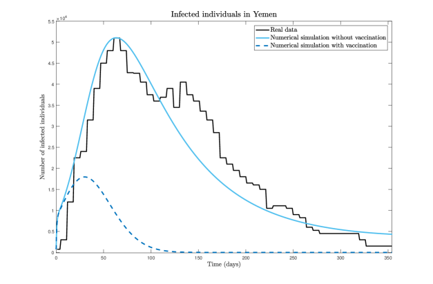
Figure 1: Numerical solution of model (2.1)–(3.1) with the parameters of Table 2 without (blue solid line) and with (blue dashed line) vaccination and real data (black solid line) of infected individuals $I(t)$ in Yemen from 27${}^{\text{th}}$ April 2017 to 15${}^{\text{th}}$ April 2018.

Table 2: Parameter values and initial conditions for the SIQRVB model (2.1).

Parameter	Description	Value	Reference
$\Lambda$	Recruitment rate	28.4$N(0)$/365000 (day-1)	[12]
$\mu$	Natural death rate	1.6$\times 10^{-5}$ (day-1)	[13]
$\beta$	Ingestion rate	0.01694 (day-1)	Assumed
$\kappa$	Half saturation constant	$10^{7}$ (cell/ml)	Assumed
$\omega_{1}$	Immunity waning rate	0.4/365 (day-1)	[19]
$\omega_{2}$	Efficacy vaccination waning rate	1/1 460 (day-1)	[7]
$\varphi$	Vaccination rate	5/1 000 (day-1)	Assumed
$\delta$	Treatment rate	1.15 (day-1)	Assumed
$\varepsilon$	Recovery rate	0.2 (day-1)	[18]
$\alpha_{1}$	Death rate (infected)	6$\times 10^{-6}$ (day-1)	[13, 31]
$\alpha_{2}$	Death rate (in treatment)	3$\times 10^{-6}$ (day-1)	Assumed
$\eta$	Shedding rate (infected)	10 (cell/ml day-1 person-1)	[3]
$d$	Bacteria death rate	0.33 (day-1)	[3]
$S(0)$	Susceptible individuals at $t=0$	28 249 670 (person)	[34]
$I(0)$	Infected individuals at $t=0$	750 (person)	[31]
$T(0)$	Treated individuals at $t=0$	0 (person)	Assumed
$R(0)$	Recovered individuals at $t=0$	0 (person)	Assumed
$V(0)$	Vaccinated individuals at $t=0$	0 (person)	[30]
$B(0)$	Bacterial concentration at $t=0$	$275\times 10^{3}$ (cell/ml)	Assumed

5 Conclusion

In this paper, we proposed and analysed, analytically and numerically, a SITRVB model for cholera transmission dynamics. In order to fit the biggest cholera outbreak worldwide, which has occurred very recently in Yemen, we simulated the outbreak of Yemen without vaccination. Indeed, vaccination did not exist in Yemen from 27${}^{\text{th}}$ April 2017 to 15${}^{\text{th}}$ April 2018. Simulations of our mathematical model, with and without vaccination, show that the introduction of vaccination from the beginning of the epidemic could have changed the situation in Yemen substantially, to the case $R_{0}<1$, where the disease extinguishes naturally. Therefore, our research motivates and fortify the importance of vaccination in cholera epidemics.

Conflict of Interest

The authors declare that there is no conflicts of interest in this paper.

References

• 1 Asian Scientist: Math in a time of cholera, 30${}^{\text{th}}$ August 2017, https://www.asianscientist.com/2017/08/health/mathematical-model-yemen-cholera-outbreak/
• 2 V. Capasso and S. L. Paveri-Fontana (1979), A mathematical model for the 1973 cholera epidemic in the European Mediterranean region, Rev. Epidemiol. Sante, 27, 121–132.
• 3 F. Capone, V. De Cataldis and R. De Luca (2015), Influence of diffusion on the stability of equilibria in a reactiondiffusion system modeling cholera dynamic, J. Math. Biol., 71, 1107–1131.
• 4 J. Carr (1981), Applications Centre Manifold Theory, Springer-Verlag: New York.
• 5 C. Castillo-Chavez and B. Song (2004), Dynamical models of tuberculosis and their applications, Math. Biosci. Eng., 1, 361–404.
• 6 N. Chitnis, J. M. Hyman and J. M. Cushing (2008), Determining important parameters in the spread of malaria through the sensitivity analysis of a mathematical model, Bull. Math. Bio., 70, 1272–1296.
• 7 Cholera vaccine, 06${}^{\text{th}}$ June 2018, https://en.wikipedia.org/wiki/Cholera_vaccine
• 8 C. T. Codeço (2001), Endemic and epidemic dynamics of cholera: the role of the aquatic reservoir, BMC Infect. Dis., 1, 14 pp.
• 9 D. M. Hartley, J. B. Morris and D. L. Smith (2006), Hyperinfectivity: a critical element in the ability of V. cholerae to cause epidemics, Plos Med., 3(1): e7.
• 10 H. W. Hethcote (2000), The mathematics of infectious diseases, SIAM Rev., 42, 599–653.
• 11 S. D. Hove-Musekwa, F. Nyabadza, C. Chiyaka, P. Das, A. Tripathi and Z. Mukandavire (2010), Modelling and analysis of the effects of malnutrition in the spread of cholera, Math. Comput. Modelling, 53, 1583–1595.
• 12 Index Mundi, Birth rate of Yemen, 06${}^{\text{th}}$ June 2018, https://www.indexmundi.com/g/g.aspx?c=ym&v=25
• 13 Index Mundi, Death rate of Yemen, 06${}^{\text{th}}$ June 2018, https://www.indexmundi.com/g/g.aspx?c=ym&v=26
• 14 R. I. Joh, H. Wang, H. Weiss and J. S. Weitza (2009), Dynamics of indirectly transmitted infectious diseases with immunological threshold, Bull. Math. Biol., 71, 845–862.
• 15 Q. Kong, Z. Qiu, Z. Sang and Y. Zou (2011), Optimal control of a vector-host epidemics model, Math. Control Relat. Fields, 1, 493–508.
• 16 A. P. Lemos-Paião, C. J. Silva and D. F. M. Torres (2017), An epidemic model for cholera with optimal control treatment, J. Comput. Appl. Math., 318, 168–180. \arXiv1611.02195
• 17 Z. Mukandavire, F. K. Mutasa, S. D. Hove-Musekwa, S. Dube and J. M. Tchuenche (2008), Mathematical analysis of a cholera model with carriers and assessing the effects of treatment, In: Wilson, L.B. (Ed.), Mathematical Biology Research Trends. Nova Science Publishers, pp. 1–37.
• 18 A. Mwasa and J. M. Tchuenche (2011), Mathematical analysis of a cholera model with public health interventions, Bull. Math. Biol., 105, 190–200.
• 19 R. L. M. Neilan, E. Schaefer, H. Gaff, K. R. Fister and S. Lenhart (2010), Modeling optimal intervention strategies for cholera, Bull. Math. Biol., 72, 2004–2018.
• 20 H. Nishiura, S. Tsuzuki, B. Yuan, T. Yamaguchi and Y. Asai (2017), Transmission dynamics of cholera in Yemen, 2017: a real time forecasting Theor. Biol. Med. Model., 14, 8 pp.
• 21 G. J. Olsder and J. W. van der Woude (2005), Mathematical Systems Theory, VSSD: Delft.
• 22 M. Pascual, L. F. Chaves, B. Cash, X. Rodo and M. D. Yunus (2008), Predicting endemic cholera: the role of climate variability and disease dynamics, Climate Res., 36, 131–140.
• 23 Reuters, Cholera vaccination campaign starts in Yemen after year delay: WHO, 07${}^{\text{th}}$ May 2018, Available from: https://www.reuters.com/article/us-health-cholera/cholera-vaccination-campaign-starts-in-yemen-after-year-delay-who-idUSKBN1I8162
• 24 Z. Shuai, J. H. Tien and P. van den Driessche (2012), Cholera models with hyperinfectivity and temporary immunity, Bull. Math. Biol., 74, 2423–2445.
• 25 C. J. Silva and D. F. M. Torres (2013), Optimal control for a tuberculosis model with reinfection and post-exposure interventions, Math. Biosci., 244, 154–164. \arXiv1305.2145
• 26 The Telegraph News, ’Race against time’ to curb cholera outbreak in Yemen, 09${}^{\text{th}}$ May 2018, https://www.telegraph.co.uk/news/0/race-against-time-curb-cholera-outbreak-yemen/
• 27 P. van den Driessche and J. Watmough (2002), Reproduction numbers and subthreshold endemic equilibria for compartmental models of disease transmission, Math. Biosc., 180, 29–48.
• 28 Wikipedia, 2016–2018 Yemen Cholera Outbreak, 08${}^{\text{th}}$ June 2018, http://en.m.wikipedia.org/wiki/2016-18_Yemen_cholera_outbreak
• 29 World Health Organization, Yemen cholera situation report no. 4, 19${}^{\text{th}}$ July 2017, http://www.emro.who.int/images/stories/20170719_WHO_cholera_SitRep_4_v2.pdf?ua=1
• 30 World Health Organization, Yemen crisis, Fighting the world’s largest cholera outbreak: oral cholera vaccination campaign begins in Yemen, 06${}^{\text{th}}$ June 2018, http://www.emro.who.int/pdf/yem/yemen-news/oral-cholera-vaccination-campaign-in-yemen-begins.pdf?ua=1
• 31 World Health Organization, Yemen: Weekly Cholera Bulletins, 21${}^{\text{st}}$ May 2018, http://www.emro.who.int/yem/yemeninfocus/situation-reports.html
• 32 World Health Organization, Yemen: Weekly Epidemiological Bulletin W15 2018, 21${}^{\text{st}}$ May 2018, http://www.emro.who.int/images/stories/yemen/week_15.pdf?ua=1
• 33 X. Yang, L. Chen and J. Chen (1996), Permanence and positive periodic solution for the single-species nonautonomous delay diffusive models, Comput. Math. Appl., 32, 109–116.
• 34 Yemen population, 06${}^{\text{th}}$ June 2018, http://www.worldometers.info/world-population/yemen-population/