Point Cloud GAN

Abstract

Generative Adversarial Networks (GAN) can achieve promising performance on learning complex data distributions on different types of data. In this paper, we first show a straightforward extension of existing GAN algorithm is not applicable to point clouds, because the constraint required for discriminators is undefined for set data. We propose a two fold modification to GAN algorithm for learning to generate point clouds (PC-GAN). First, we combine ideas from hierarchical Bayesian modeling and implicit generative models by learning a hierarchical and interpretable sampling process. A key component of our method is that we train a posterior inference network for the hidden variables. Second, instead of using only state-of-the-art Wasserstein GAN objective, we propose a sandwiching objective, which results in a tighter Wasserstein distance estimate than the commonly used dual form. Thereby, PC-GAN defines a generic framework that can incorporate many existing GAN algorithms. We validate our claims on ModelNet40 benchmark dataset. Using the distance between generated point clouds and true meshes as metric, we find that PC-GAN trained by the sandwiching objective achieves better results on test data than the existing methods. Moreover, as a byproduct, PC-GAN learns versatile latent representations of point clouds, which can achieve competitive performance with other unsupervised learning algorithms on object recognition task. Lastly, we also provide studies on generating unseen classes of objects and transforming image to point cloud, which demonstrates the compelling generalization capability and potentials of PC-GAN.

1 Introduction

A fundamental problem in machine learning is: given a data set, learn a generative model that can efficiently generate arbitrary many new sample points from the domain of the underlying distribution (Bishop, 2006). Deep generative models use deep neural networks as a tool for learning complex data distributions (Kingma and Welling, 2013; Oord et al., 2016; Goodfellow et al., 2014). Especially, Generative Adversarial Networks (GAN; Goodfellow et al. 2014) is drawing attentions because of its success in many applications. Compelling results have been demonstrated on different types of data, including text, images and videos (Lamb et al., 2016; Karras et al., 2017; Vondrick et al., 2016). Their wide range of applicability was also shown in many important problems, including data augmentation (Salimans et al., 2016), image style transformation (Zhu et al., 2017), image captioning (Dai et al., 2017) and art creations (Kang, 2017).

Recently, capturing 3D information is garnering attention. There are many different data types for 3D information, such as CAD, 3D meshes and point clouds. 3D point clouds are getting popular since these store more information than 2D images and sensors capable of collecting point clouds have become more accessible. These include Lidar on self-driving cars, Kinect for Xbox and face identification sensor on phones. Compared to other formats, point clouds can be easily represented as a set of points, which has several advantages, such as permutation invariance. The algorithms which can effectively learn from this type of data is an emerging field (Qi et al., 2017a, b; Zaheer et al., 2017; Kalogerakis et al., 2017; Fan et al., 2017). However, compared to supervised learning, unsupervised generative models for 3D data are still under explored (Achlioptas et al., 2017; Oliva et al., 2018).

Extending existing GAN frameworks to handle 3D point clouds, or more generally set data, is not straightforward. In this paper, we begin by formally defining the problem and discussing the difficulty of the problem (Section 2). Circumventing the challenges, we propose a deep generative adversarial network (PC-GAN) with a hierarchical sampling and inference network for point clouds. The proposed architecture learns a stochastic procedure which can generate new point clouds as well as draw samples from point clouds without explicitly modeling the underlying density function (Section 3). The proposed PC-GAN is a generic algorithm which can incorporate many existing GAN variants. By utilizing the property of point clouds, we further propose a sandwiching objective by considering both upper and lower bounds of Wasserstein distance estimate, which can lead to tighter approximation (Section 4). Evaluation on ModelNet40 shows excellent generalization capability of PC-GAN. We first show we can sample from the learned model to generate new point clouds and the latent representations learned by the inference network provide meaningful interpolations between point clouds. We further show the conditional generation results on unseen classes of objects to demonstrate the superior generalization ability of PC-GAN. Lastly, we also provide several interesting studies, such as classification and point clouds generation from images (Section 6).

2 Problem Definition and Difficulty

We begin by defining the problem and ideal generative process for point cloud over objects. Formally, a point cloud for an object $\theta$ is a set of $n$ low dimensional vectors $X=\{x_{1},...,x_{n}\}$ with $x_{i}\in\mathbb{R}^{d}$, where $d$ is usually $3$ and $n$ can be infinite. Point cloud for $M$ different objects is a collection of $M$ sets $X^{(1)},...,X^{(M)}$, where each $X^{(m)}$ is as defined above. Thus, we basically need a generative model $p(X)$ for sets which should be able to:

• Sample entirely new sets $X$, as well as

• Sample more points for a given set, i.e. $x\sim p(x|X)$.

De-Finetti theorem allows us to express the set probability in a factored format as $p(X)=\int_{\theta}\prod_{i=1}^{n}p(x_{i}|\theta)p(\theta)d\theta$ for some suitably defined $\theta$. In case of point clouds, the latent variable

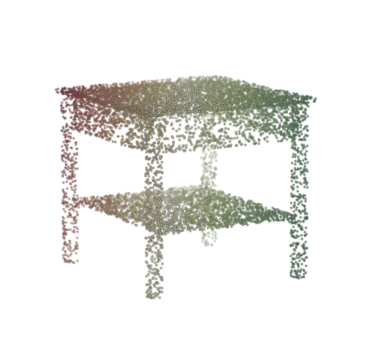
(a) Table: $p(x_{i}|\theta_{1})$

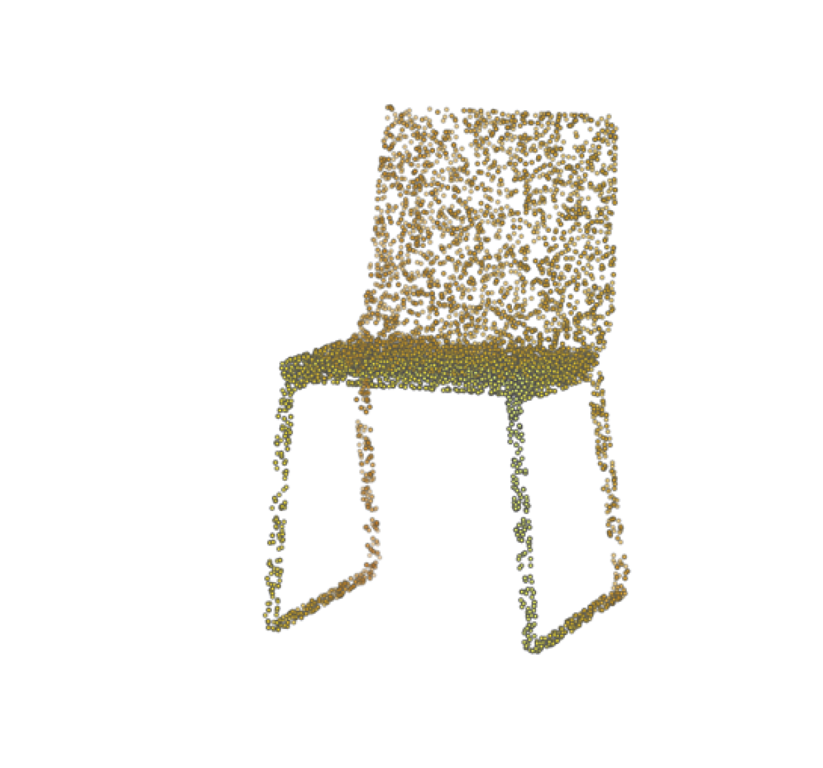
(b) Chair: $p(x_{i}|\theta_{2})$

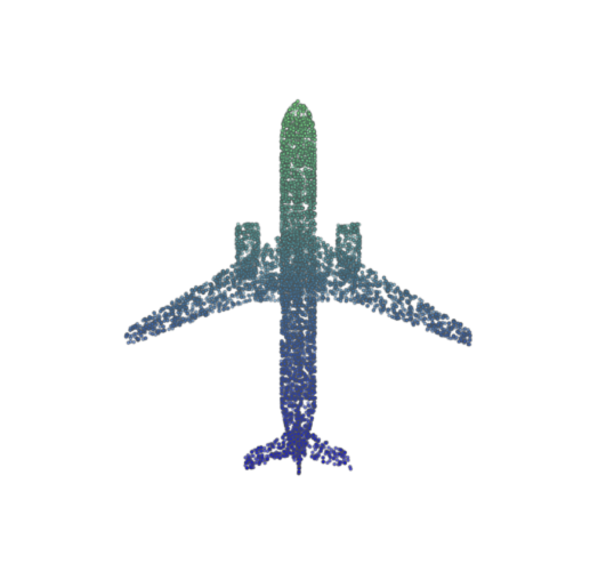
(c) Plane: $p(x_{i}|\theta_{3})$

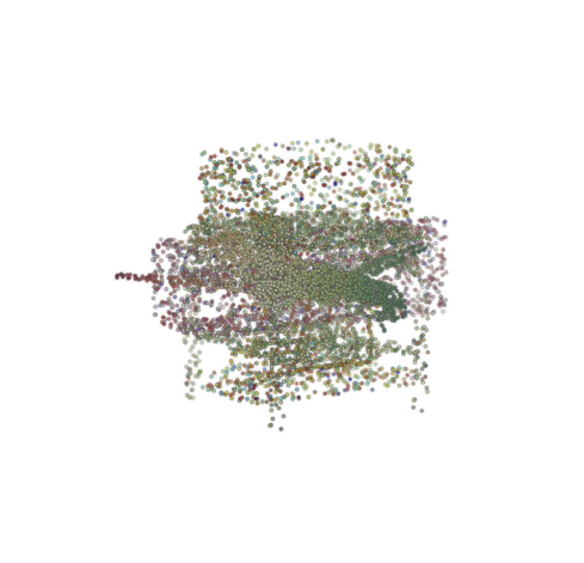
(d) Marginalized: $p(x_{i})$

Figure 1: Unlike in case of images, the marginal distribution $p(x_{i})=\int p(x_{i}|\theta)p(\theta)d\theta$ is not useful. We have to learn the joint distribution $p(X,\theta)$. An illustrative parallel can be drawn between pixels of an image and point cloud — marginal distribution of pixels is quite uninformative, one has to consider the joint distribution of all pixels in one image (not across different images).

$\theta$ can be interpreted as an object representation. In this view, the factoring can be understood as follows: Given an object, $\theta$, the points $x_{i}$ in the point cloud can be considered as i.i.d. samples from $p(x|\theta)$, an unknown latent distribution representing object $\theta$. Joint likelihood can be expressed as:

$$p(X,\theta)=\underbrace{p(\theta)}_{\text{object}}\;\;\;\underbrace{\prod_{i=1}^{n}p(x_{i}|\theta)}_{\text{points for object}}$$ (1)

Attempts have been made to characterize (1) with parametric models like Gaussian Mixture Models or parametric hierarchical models (Jian and Vemuri, 2005; Strom et al., 2010; Eckart et al., 2015). However, such approaches have limited success as the point cloud conditional density $p(x|\theta)$ is highly non-linear and complicated (example of point clouds can be seen in Figure 1, 3, 7).

With advent of implicit generative models, like GANs (Goodfellow et al., 2014), it is possible to model complicated distributions, but it is not clear how to extend the existing GAN frameworks to handle the hierarchical model of point clouds as developed above. The aim of most GAN framework(Goodfellow et al., 2014; Arjovsky et al., 2017; Li et al., 2017a) is to learn to generate new samples from a distribution $p(x)$, for fixed dimensional $x\in\mathbb{R}^{d}$, given a training dataset. We, in contrast, aim to develop a new method where the training data is a set of sets, and learning from this training data would allow us to generate points from this hierarchical distribution (e.g. point clouds of 3D objects). To re-emphasize the incompatibility, note that the training data of traditional GANs is a set of fixed dimensional instances, in our case, however, it is a set of sets. Using existing GANs to just learning marginal distribution $p(x)$, in case of point clouds $x$, is not of much use because the marginal distribution is quite uninformative as can be seen from Figure 1.

One approach can be used to model the distribution of the point cloud set together, i.e., $\{\{x_{i}^{(1)}\}_{i=1}^{n},\dots,\{x_{i}^{(m)}\}_{i=1}^{n}\}$. In this setting, a naíve application of traditional GAN is possible through treating the point cloud as finite dimensional vector by fixing number and order of the points (reducing the problem to instances in $\mathbb{R}^{n\times 3}$) with DeepSets (Zaheer et al., 2017) classifier as the discriminator to distinguish real sets from fake sets. However, it would not work because the IPM guarantees behind the traditional GAN no longer hold (e.g. in case of Arjovsky et al. (2017), nor are 1-Lipschitz functions over sets well-defined). The probabilistic divergence approximated by a DeepSets classifier is not clear and might be ill-defined. Counter examples for breaking IPM guarantees can be easily found as we show next.

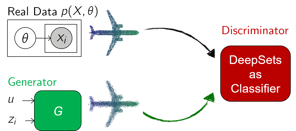
Figure 2: Natural extension of GAN to handle set data does not work.

Counter Example

Consider a simple GAN (Goodfellow et al., 2014) with a DeepSets classifier as the discriminator. In order to generate coherent sets of variable size, we consider a generator $G$ having two noise sources: $u$ and $z_{i}$. To generate a set, $u$ is sampled once and $z_{i}$ is sampled for $i=1,2,...,n$ to produce $n$ points in the generated set. Intuitively, fixing the first noise source $u$ selects a set and ensures the points generated by repeated sampling of $z_{i}$ are coherent and belong to same set. The setup is depicted in Figure 2. In this setup, the GAN minimax problem would be:

$$\min_{G}\max_{D}\underset{\begin{subarray}{c}\theta\sim p(\theta)\\ x_{i}\sim p(x_{i}|\theta)\end{subarray}}{\mathbb{E}}\left[\log D\left(\{x_{i}\}\right)\right]\;+\underset{\begin{subarray}{c}u\sim p(u)\\ z_{i}\sim p(z_{i})\end{subarray}}{\mathbb{E}}\left[\log\left(1-D\left(\{G(u,z_{i})\}\right)\right)\right]$$ (2)

Now consider the case, when there exist an ‘oracle’ mapping $T$ which maps each sample point deterministically to the object it originated from, i.e. $\exists T:T(\{x_{i}\})=\theta$. A valid example is when different $\theta$ leads to conditional distribution $p(x|\theta)$ with non-overlapping support. Let $D=D^{\prime}\circ T$ and $G$ ignores $z$ then optimization becomes

$$\min_{G}\max_{D^{\prime}}\underset{\begin{subarray}{c}\theta\sim p(\theta)\\ x_{i}\sim p(x_{i}|\theta)\end{subarray}}{\mathbb{E}}\left[\log D^{\prime}\left(T\left(\{x_{i}\}\right)\right)\right]\;+\underset{\begin{subarray}{c}u\sim p(u)\\ z_{i}\sim p(z_{i})\end{subarray}}{\mathbb{E}}\left[\log\left(1-D^{\prime}\left(T\left(\{G(u,z_{i})\}\right)\right)\right)\right]$$ (3)

$$\Rightarrow \min_{G}\max_{D^{\prime}}\underset{\begin{subarray}{c}\theta\sim p(\theta)\\ x_{i}\sim p(x_{i}|\theta)\end{subarray}}{\mathbb{E}}\left[\log D^{\prime}\left(\theta\right)\right]\;+\underset{\begin{subarray}{c}u\sim p(u)\\ z_{i}\sim p(z_{i})\end{subarray}}{\mathbb{E}}\left[\log\left(1-D^{\prime}\left(T\left(\{G(u)\}\right)\right)\right)\right]$$

$$\Rightarrow \min_{G}\max_{D^{\prime}}\underset{\begin{subarray}{c}\theta\sim p(\theta)\end{subarray}}{\mathbb{E}}\left[\log D^{\prime}\left(\theta\right)\right]\;+\underset{\begin{subarray}{c}u\sim p(u)\end{subarray}}{\mathbb{E}}\left[\log\left(1-D^{\prime}\left(T\left(\{G(u)\}\right)\right)\right)\right]$$

Thus, we can achieve the lower bound $-\log(4)$ by only matching the $p(\theta)$ component, while the conditional $p(x|\theta)$ is allowed to remain arbitrary. We note that there still exists good solutions, which can lead to successful training, other than this hand-crafted example. We found empirically that GAN with simple DeepSet-like discriminator most of the times fails to learn to generate point clouds even after converging. However, sometimes it does results in reasonable generations. So simply using DeepSets classifier without any constraints in simple GAN in order to handle sets does not always lead to a valid generative model. We need additional constraints for GANs with simple DeepSet-like discriminator to exclude such bad solutions and lead to a more stable training.

3 Proposed Method

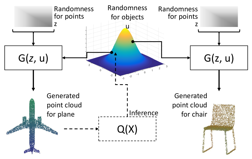
Figure 3: Overview of PC-GAN.

Although directly learning point cloud generation under GAN formulation is difficult as described in Section 2, given a $\theta$, learning $p(X|\theta)$ is reduced to learning a 2 or 3 dimensional distribution, which fits standard GAN settings. Formally, given a $\theta$, we train a generator $G_{x|\theta}(z)$ such that $x=G_{x|\theta}(z)$, where $z\sim p(z)$, follows $\mathbb{G}$ by optimizing a (peudo) probabilistic divergence $D(\mathbb{P}\|\mathbb{G})$ between the distribution $\mathbb{G}$ of $G_{x|\theta}(z)$ and $p(x|\theta)$, which is denoted as $\mathbb{P}$. The full objective can be written as $\displaystyle\mathbb{E}_{\theta\sim p(\theta)}\bigg{[}\min_{G_{x}}D(\mathbb{P}\|\mathbb{G})\bigg{]}$.

Inference

Although GANs have been extended to learn conditional distributions (Mirza and Osindero, 2014; Isola et al., 2017), they require conditioning variables to be observed, such as the one-hot label or a given image. While in case of point clouds we only have partial knowledge of the conditional, i.e. we only have groupings of point coming from the same object but we have no representation $\theta$ of the conditional or the object other than the points themselves. Naïvely modeling $\theta$ to be a one-hot vector, to indicate which object the points belong to in the training data, cannot generalize to unseen testing data. Instead, we need a richer representation for $\theta$, which is an unobserved random variable. Thus, we need to infer $\theta$ during the training. The proposed algorithm has to concurrently learn the inference network $Q(X)$ which encodes $\theta$ while we learn $p(x|\theta)$.

Neural Network Realization

Our solution comprises of a generator $G_{x}(z,\psi)$ which takes in a noise source $z\in\mathbb{R}^{d_{1}}$ and a descriptor $\psi\in\mathbb{R}^{d_{2}}$ encoding information about distribution of $\theta$. Here $d_{1}$ is dimensionality of the per-point noise source $z$ and $d_{2}$ is the size of the descriptor vector. Typically, we would need $d_{1}\ll d_{2}$, as $psi$ needs to encode much more information because it decides the whole shape of the conditional distribution whereas $z$ just corresponds to different samples from it. Another interpretation of the descriptor $\psi$ can be as an embedding of distribution over $\theta$. For a given $\theta_{0}$, the descriptor $\psi$ would encode information about the distribution $\delta(\theta-\theta_{0})$ and samples generated as $x=G_{x}(z,\psi)$ would follow the distribution $p(x|\theta_{0})$. More generally, $\psi$ can be used to encode more complicated distributions regarding $\theta$ as well. In particular, it could be used to encode the posterior $p(\theta|X)$ for a given sample set $X$, such that $x=G_{x}(z,\psi)$ follows the posterior predictive distribution:

$$p(x|X)=\int p(x|\theta)p(\theta|X)d\theta.$$

As $\psi$ is unobserved, we use an inference network $Q(X)$ to learn the most informative descriptor $\psi$ about the distribution $p(\theta|X)$ to minimize the The divergence between $p(X|\theta)$, which is denoted as $\mathbb{P}$, and the distribution of $G_{x}(z,Q(X))$ given $Q(X)$, which we abuse $\mathbb{G}$ for convenience, that is $\displaystyle\mathbb{E}_{\theta\sim p(\theta)}\bigg{[}\min_{G_{x},Q}D(\mathbb{P}\|\mathbb{G})\bigg{]}$.

A major hurdle in taking this path is that $X$ is a set of points, which can vary in size and permutation of elements. Thus, making design of $Q$ complicated as traditional neural network can not handle this and possibly is the reason for absence of such framework in the literature despite being a natural solution for the important problem of generative modeling of point clouds. However, we can overcome this challenge and we propose to construct the inference network by utilizing the recent advance in deep learning for dealing with sets (Qi et al., 2017a; Zaheer et al., 2017). This allows it handle variable number of inputs points in arbitrary order, yet yielding a consistent descriptor $\psi$.

Hierarchical Sampling

After training $G_{x}$ and $Q$, we use trained $Q$ to collect inferred $Q(X)$ and train another generator $G_{\theta}(u)\sim p(\psi)$ for higher hierarchical sampling. Here $u\in\mathbb{R}^{d_{3}}$ is the other noise source independent of $z$ and dimensionality $d_{3}$ this noise source is typically much smaller than $d_{2}$. In addition to layer-wise training, a joint training could further boost performance. The full generative process for sampling one point cloud could be represented as

$$\{x_{i}\}_{i=1}^{n}=\{G(z_{i},u)\}_{i=1}^{n}=\{G_{x}(z_{i},G_{\theta}(u))\}_{i=1}^{n},\mbox{ where }z_{1},\dots,z_{n}\sim p(z),\mbox{ and }u\sim p(u).$$

We call the proposed algorithm for point cloud generation as PC-GAN as shown in Figure 3. The conditional distribution matching with a learned inference in PC-GAN can also be interpreted as an encoder-decoder formulation (Kingma and Welling, 2013). The difference between it and the point cloud autoencoder (Achlioptas et al., 2017; Yang et al., 2018) will be discussed in Section 5.

4 Different Divergences for Matching Point Clouds

Given two point clouds $x\sim p(X|\theta)$ and $G_{x}(z,Q(X))$, one commonly used heuristic distance measure is chamfer distance (Achlioptas et al., 2017). On the other hand, if we treat each point cloud as a 3 dimensional distribution, we can adopt a more broader classes of probabilistic divergence $D(\mathbb{P}\|\mathbb{G})$ for training $G_{x}$. Instead of using divergence esitmates which requires density estimation (Jian and Vemuri, 2005; Strom et al., 2010; Eckart et al., 2015), we are interested in implicit generative models with a GAN-like objective (Goodfellow et al., 2014), which has been demonstrated to learn complicated distributions.

To train the generator $G_{x}$ using a GAN-like objective for point clouds, we need a discriminator $f(\cdot)$ which distinguishes between the generated samples and true samples conditioned on $\theta$. Combining with the inference network discussed in Section 3, if we use an IPM-based GAN (Arjovsky et al., 2017; Mroueh and Sercu, 2017; Mroueh et al., 2017), the objective can be written as

$$\mathbb{E}_{\theta\sim p(\theta)}\bigg{[}\min_{G_{x},Q}\underbrace{\max_{f\in\Omega_{f}}\mathbb{E}_{x\sim p(X|\theta)}\left[f(x)\right]-\mathbb{E}_{z\sim p(z),X\sim p(X|\theta)}\left[f(G_{x}(z,Q(X)))\right]}_{D(\mathbb{P}\|\mathbb{G})}\bigg{]},$$ (4)

where $\Omega_{f}$ is the constraint for different probabilistic distances, such as 1-Lipschitz (Arjovsky et al., 2017), $L^{2}$ ball (Mroueh and Sercu, 2017) or Sobolev ball (Mroueh et al., 2017).

4.1 Tighter Solutions via Sandwiching

In our setting, each point $x_{i}$ in the point cloud can be considered to correspond to single images when we train GANs over images. An example is illustrated in Figure 4, where the samples from MMD-GAN (Li et al., 2017a) trained on CelebA consists of both good and bad faces. In case of images, when quality is evaluated, it primarily focuses on coherence individual images and the few bad ones are usually left out. Whereas in case of point cloud, to get representation of an object we need many sampled points together and presence of outlier points degrades the quality of the object. Thus, when training a generative model for point cloud, we need to ensure a much lower distance $D(\mathbb{P}\|\mathbb{G})$ between true distribution $\mathbb{P}$ and generator distribution $\mathbb{G}$ than would be needed for images.

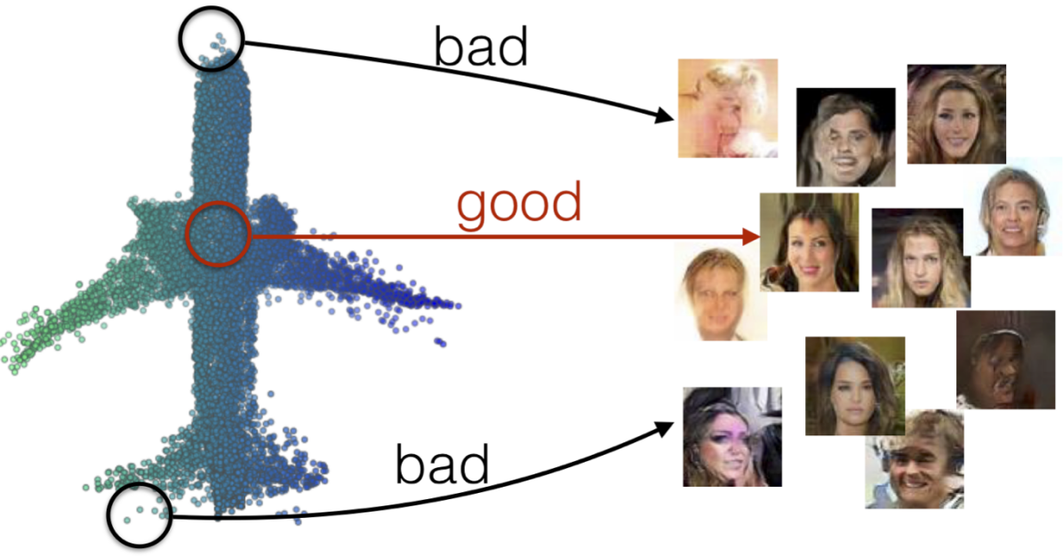
Figure 4: Connection between good/bad points and faces generated from a GAN.

We begin by noting that the popular Wasserstein GAN (Arjovsky et al., 2017), aims to optimize $G$ by $\min w(\mathbb{P},\mathbb{G})$, where $w(\mathbb{P},\mathbb{G})$ is the Wasserstein distance $w(\mathbb{P},\mathbb{G})$ between the truth $\mathbb{P}$ and generated distribution $\mathbb{G}$ of $G$. Many GAN works (e.g. Arjovsky et al. (2017)) approximate $w(\mathbb{P},\mathbb{G})$ in dual form (a maximization problem), such as (4), by neural networks. The resulting estimate $W_{L}(\mathbb{P},\mathbb{G})$ is a lower bound of the true Wasserstein distance, as neural networks can only recover a subset of 1-Lipschitz functions (Arora et al., 2017) required in the dual form. However, finding a lower bound $W_{L}(\mathbb{P},\mathbb{G})$ for $w(\mathbb{P},\mathbb{G})$ may not be an ideal surrogate for solving a minimization problem $\min w(\mathbb{P},\mathbb{G})$. In optimal transport literature, Wassertein distance is usually estimated by approximate matching cost, $W_{U}(\mathbb{P},\mathbb{G})$, which gives us an upper bound of the true Wasserstein distance.

We propose to combine, in general, a lower bound and upper bound estimate by sandwiching the solution between the two, i.e. we solve the following minimization problem:

$$\min_{G} W_{U}(\mathbb{P},\mathbb{G})$$ (5)

such that $$W_{U}(\mathbb{P},\mathbb{G})-W_{L}(\mathbb{P},\mathbb{G})<\lambda$$

The problem can be simplified and solved using method of Lagrange multipliers as follows:

$$\min_{G}W_{\lambda}(\mathbb{P},\mathbb{G}):=(1-\lambda)W_{U}(\mathbb{P},\mathbb{G})+\lambda W_{L}(\mathbb{P},\mathbb{G})$$ (6)

By solving the new sandwiched problem (6), we show that under certain conditions we obtain a better estimate of Wasserstein distance in the following lemma:

Lemma 1.

Suppose we have two approximators to Wasserstein distance: an upper bound $W_{U}$ and a lower $W_{L}$, such that $\forall P,G:(1+\epsilon_{1})w(\mathbb{P},\mathbb{G})\leq W_{U}(\mathbb{P},\mathbb{G})\leq(1+\epsilon_{2})w(\mathbb{P},\mathbb{G})$ and $\forall P,G:(1-\epsilon_{2})w(\mathbb{P},\mathbb{G})\leq W_{L}(\mathbb{P},\mathbb{G})\leq(1-\epsilon 1)w(\mathbb{P},\mathbb{G})$ respectively, for some $\epsilon_{2}>\epsilon_{1}>0$ and $\epsilon_{1}>\epsilon_{2}/3$. Then, using the sandwiched estimator $W_{\lambda}$ from (6), we can achieve tighter estimate of the Wasserstein distance than using either one estimator, i.e.

$$\exists\lambda:|W_{\lambda}(\mathbb{P},\mathbb{G})-w(\mathbb{P},\mathbb{G})|<\min\{|W_{U}(\mathbb{P},\mathbb{G})-w(\mathbb{P},\mathbb{G})|,|W_{L}(\mathbb{P},\mathbb{G})-w(\mathbb{P},\mathbb{G})|\}$$ (7)

4.1.1 Upper Bound Implementation

The primal form of Wasserstein distance is defined as

$$w(\mathbb{P},\mathbb{G})=\inf_{\gamma\in\Gamma(\mathbb{P},\mathbb{G})}\int\|x-y\|_{1}d\gamma(x,y),$$

where $\gamma$ is the coupling of $P$ and $G$. The Wasserstein distance is also known as optimal transport (OT) or earth moving distance (EMD). As the name suggests, when $w(\mathbb{P},\mathbb{G})$ is estimated with finite number of samples $X={x_{1},\dots,x_{n}}$ and $Y={y_{1},\dots,y_{n}}$, we find the one-to-one matching between $X$ and $Y$ such that the total pairwise distance is minimal. The resulting minimal total (average) pairwise distance is $w(X,Y)$. In practice, finding the exact matching efficiently is non-trivial and still an open research problem (Peyré et al., 2017). Instead, we consider an approximation provided by Bertsekas (1985). It is an iterative algorithm where each iteration operates like an auction whereby unassigned points $x\in X$ bid simultaneously for closest points $y\in Y$, thereby raising their prices. Once all bids are in, points are awarded to the highest bidder. The crux of the algorithm lies in designing a non-greedy bidding strategy. One can see by construction the algorithm is embarrassingly parallelizable, which is favourable for GPU implementation. One can show that algorithm terminates with a valid matching and the resulting matching cost $W_{U}(X,Y)$ is an $\epsilon$-approximation of $w(X,Y)$. Thus, the estimate can serve as an upper bound, i.e.

$$w(X,Y)\leq W_{U}(X,Y)\leq(1+\epsilon)w(X,Y),$$ (8)

We remark estimating Wasserstein distance $w(\mathbb{P},\mathbb{G})$ with finite samples via primal form is only favorable to low dimensional data, such as point clouds. The error of empirical estimate in primal is $O(1/n^{1/d})$ (Weed and Bach, 2017). When the dimension $d$ is large (e.g. images), we cannot accurately estimate $w(\mathbb{P},\mathbb{G})$ in primal as well as its upper bound with a small minibatch.

Finding a modified primal form with low sample complexity, especially for high dimensional data, is still an open research problem (Cuturi, 2013; Genevay et al., 2018). Combining those into the proposed sandwiching objective for high dimensional data is left for future works.

4.2 Lower Bound Implementation

The dual form of Wasserstein distance is defined as

$$w(\mathbb{P},\mathbb{G})=\sup_{f\in\mathcal{L}_{1}}\mathbb{E}_{x\sim P}f(x)-\mathbb{E}_{x\sim G}f(x),$$ (9)

where $\mathcal{L}_{k}$ is the set of $k$-Lipschitz functions whose Lipschitz constant is no larger than $k$. In practice, deep neural networks parameterized by $\phi$ with constraints $f_{\phi}\in\Omega_{\phi}$ (Arjovsky et al., 2017), result in a distance approximation

$$W_{L}(\mathbb{P},\mathbb{G})=\max_{f_{\phi}\in\Omega_{\phi}}\mathbb{E}_{x\sim P}f_{\phi}(x)-\mathbb{E}_{x\sim G}f_{\phi}(x).$$ (10)

If there exists $k$ such that $\Omega_{f}\subseteq\mathcal{L}_{k}$, then $W_{L}(\mathbb{P},\mathbb{G})/k\leq w(\mathbb{P},\mathbb{G})~{}\forall P,G$ is a lower bound. To enforce $\Omega_{\phi}\subseteq\mathcal{L}_{k}$, Arjovsky et al. (2017) propose a weight clipping constraint $\Omega_{c}$, which constrains every weight to be in $[-c,c]$ and guarantees that $\Omega_{c}\subseteq\mathcal{L}_{k}$ for some $k$. Based on Arora et al. (2017), the Lipschitz functions $\Omega_{c}$ realized by neural networks is actually $\Omega_{c}\subset\mathcal{L}_{k}$.

In practice, choosing clipping range $c$ is non-trivial. Small ranges limit the capacity of networks, while large ranges result in numerical issues during the training. On the other hand, in addition to weight clipping, several constraints (regularization) have bee proposed with better empirical performance, such as gradient penalty (Gulrajani et al., 2017) and $L^{2}$ ball (Mroueh and Sercu, 2017). However, there is no guarantee the resulted functions are still Lipschitz or the resulted distances are lower bounds of Wasserstein distance. To take the advantage of those regularization with the Lipschitz guarantee, we propose a simple variation by combining weight clipping, which always ensures Lipschitz functions.

Lemma 2.

There exists $k>0$ such that

$$\max_{f\in\Omega_{c}\cap\Omega_{\phi}}\mathbb{E}_{x\sim P}[f_{\phi}(x)]-\mathbb{E}_{x\sim G}[f_{\phi}(x)]\leq\frac{1}{k}w(\mathbb{P},\mathbb{G})$$ (11)

Note that, if $c\rightarrow\infty$, then $\Omega_{c}\cap\Omega_{\phi}=\Omega_{\phi}$. Therefore, from Proposition 2, for any regularization of discriminator (Gulrajani et al., 2017; Mroueh and Sercu, 2017; Mroueh et al., 2017), we can always combine it with a weight clipping constraint $\Omega_{c}$ to ensure a valid lower bound estimate of Wasserstein distance and enjoy the advantage that it is numerically stable when we use large $c$ compared with original weight-clipping WGAN (Arjovsky et al., 2017).

5 Related Works

Generative Adversarial Network (Goodfellow et al., 2014) aims to learn a generator that can sample data followed by the data distribution. Compelling results on learning complex data distributions with GAN have been shown on images (Karras et al., 2017), speech (Lamb et al., 2016), text (Yu et al., 2016; Hjelm et al., 2017), vedio (Vondrick et al., 2016) and 3D voxels (Wu et al., 2016). However, the GAN algorithm on 3D point cloud is still under explored (Achlioptas et al., 2017). Many alternative objectives for training GANs have been studied. Most of them are the dual form of $f$-divergence (Goodfellow et al., 2014; Mao et al., 2017; Nowozin et al., 2016), integral probability metrics (IPMs) (Zhao et al., 2016; Li et al., 2017a; Arjovsky et al., 2017; Gulrajani et al., 2017) or IPM extensions (Mroueh and Sercu, 2017; Mroueh et al., 2017). Genevay et al. (2018) learn the generative model by the approximated primal form of Wasserstein distance (Cuturi, 2013).

Instead of training a generative model on the data space directly, one popular approach is combining with autoencoder (AE), which is called adversarial autoencoder (AAE) (Makhzani et al., 2015). AAE constrain the encoded data to follow normal distribution via GAN loss, which is similar to VAE (Kingma and Welling, 2013) by replacing the KL-divergence on latent space via any GAN loss. Tolstikhin et al. (2017) provide a theoretical explanation for AAE by connecting it with the primal form of Wasserstein distance. The other variant of AAE is training the other generative model to learn the distribution of the encoded data instead of enforcing it to be similar to a known distribution (Engel et al., 2017; Kim et al., 2017). Achlioptas et al. (2017) explore a AAE variant for point cloud. They use a specially-designed encoder network (Qi et al., 2017a) for learning a compressed representation for point clouds before training GAN on the latent space. However, their decoder is restricted to be a MLP which generates $m$ fixed number of points, where $m$ has to be pre-defined. That is, the output of their decoder is fixed to be $3m$ for 3D point clouds, while the output of the proposed $G_{x}$ is only 3 dimensional and $G_{x}$ can generate arbitrarily many points by sampling different random noise $z$ as input. Yang et al. (2018); Groueix et al. (2018b) propose similar decoders to $G_{x}$ with fixed grids to break the limitation of Achlioptas et al. (2017) aforementioned, but they use heuristic Chamfer distance without any theoretical guarantee and do not exploit generative models for point clouds. The proposed PC-GAN can also be interpreted as an encoder-decoder formulation. However, the underlying interpretation is different. We start from De-Finetti theorem to learn both $p(X|\theta)$ and $p(\theta)$ with inference network interpretation of $Q$, while  Achlioptas et al. (2017) focus on learning $p(\theta)$ without modeling $p(X|\theta)$.

GAN for learning conditional distribution (conditional GAN) has been studied in images with single conditioning (Mirza and Osindero, 2014; Pathak et al., 2016; Isola et al., 2017; Chang et al., 2017) or multiple conditioning (Wang and Gupta, 2016). The case on point cloud is still under explored. Also, most of the works assume the conditioning is given (e.g. labels and base images) without learning the inference during the training. Training GAN with inference is studied by Dumoulin et al. (2016); Li et al. (2017b); however, their goal is to infer the random noise $z$ of generators instead of semantic latent variable of the data. Li et al. (2018) is a parallel work aiming to learn GAN and unseen latent variable simultaneously, but they only study image and video datasets.

Lastly, we briefly review some recent development of deep learning on point clouds. Instead of transforming into 3D voxels and projecting objects into different views to use convolution (Su et al., 2015; Maturana and Scherer, 2015; Wu et al., 2015; Qi et al., 2016; Tatarchenko et al., 2017), which have the concern of memory usage, one direction is designing permutation invaraint operation for dealing with set data directly Qi et al. (2017a); Zaheer et al. (2017); Qi et al. (2017b). Wang et al. (2018) use graph convolution (Bronstein et al., 2017) to utilize local neighborhood information. Most of the application studied by those works focus on classification and segmentation tasks, but they can be used to implement the inference network $Q$ of PC-GAN.

6 Experiments

In this section we demonstrate the point cloud generation capabilities of PC-GAN. As discussed in Section 5, we refer Achlioptas et al. (2017) as AAE as it could be treated as an AAE extension to point clouds and we use the implementation provided by the authors for experiments. The sandwitching objective $W_{s}$ for PC-GAN combines $W_{L}$ and $W_{U}$ with the mixture 1:20 without tunning for all experiment. $W_{L}$ is a GAN loss by combining Arjovsky et al. (2017) and Mroueh and Sercu (2017) and we adopt (Bertsekas, 1985) for $W_{U}$ as discussed in Section 4.2 and Section 4.1.1. We parametrize $Q$ in PC-GAN by DeepSets (Zaheer et al., 2017). The review of DeepSets is in Appendix B. Other detailed configurations of each experiment can be found in Appendix C. Next, we study both synthetic 2D point cloud and ModelNet40 benchmark datasets.

6.1 Synthetic Datasets

We created a simple 2D synthetic point cloud datasets from parametric distributions on which we can carry out thorough evaluations of the prposed PC-GAN and draw comparisons with AAE Achlioptas et al. (2017). We generate 2D point clouds for circles, where the center of circles is followed a mixture of four Gaussians with means equal to $\{\pm 16\}\times\{\pm 16\}$. The covariance matrices were set to be $16I$ and we used equal mixture weights. The radius of the circles was drawn from a uniform distribution $\mbox{\it Unif}(1.6,6.4)$. One sampled circile is shown in Figure 5(a). We sampled $10,000$ circles for the training and testing data, respectively.

For PC-GAN, the inference network $Q$ is a stack of 3 Permutation Equivariance Layers with hidden layer size to be $30$ and output size to be $15$ (e.g. $Q(X)\in\mathbb{R}^{15}$). In this experiment the total number of parameters for PC-GAN is $12K$. For AAE encoder, we follow the same setting in Achlioptas et al. (2017); for decoder, we increase it from 3 to be 4 layers with larger capacities and set output size to be $500\times 2$ dimensions for $500$ points. We consider two model configurations AAE-10 and AAE-20, which use $10$ and $20$ units for the hidden layers of AAE decoder, respectively. The total number of parameters (encoder+decoder) are $14K$ and $24K$ for AAE-10 and AAE-20, respectively. Detailed model configurations are provided in the supplementary material.

We evaluated the conditional distributions on the $10,000$ testing circles. For the proposed PC-GAN, we pass the same points into the inference network $Q$, then sample $500$ points with the conditional generator $G_{x}$ to match the output number of AAE. We measured the empirical distributions of the centers and the radius of the generated circles conditioning on the testing data for PC-GAN. Similarly, we measured the reconstructed circles of the testing data for AAE. The results are shown in Figure 5.

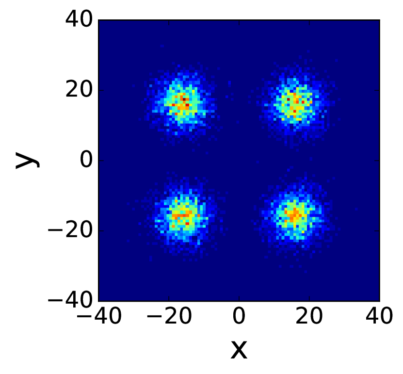
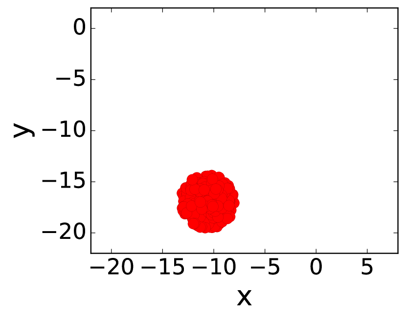
(a) True Data

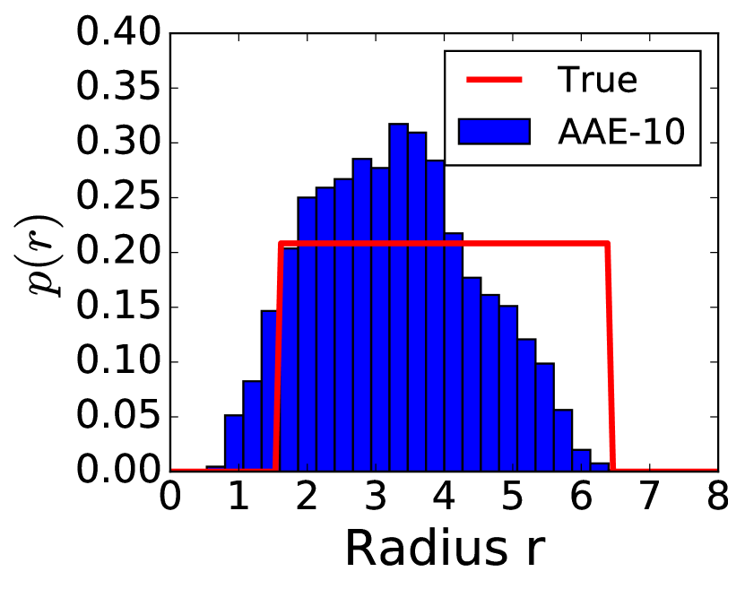
(b) AAE-10

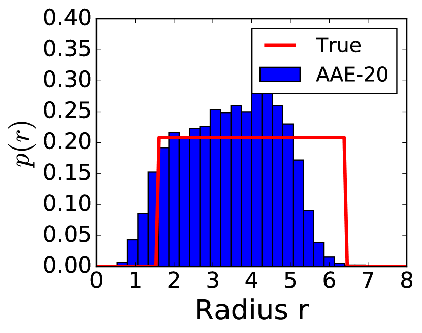
(c) AAE-20

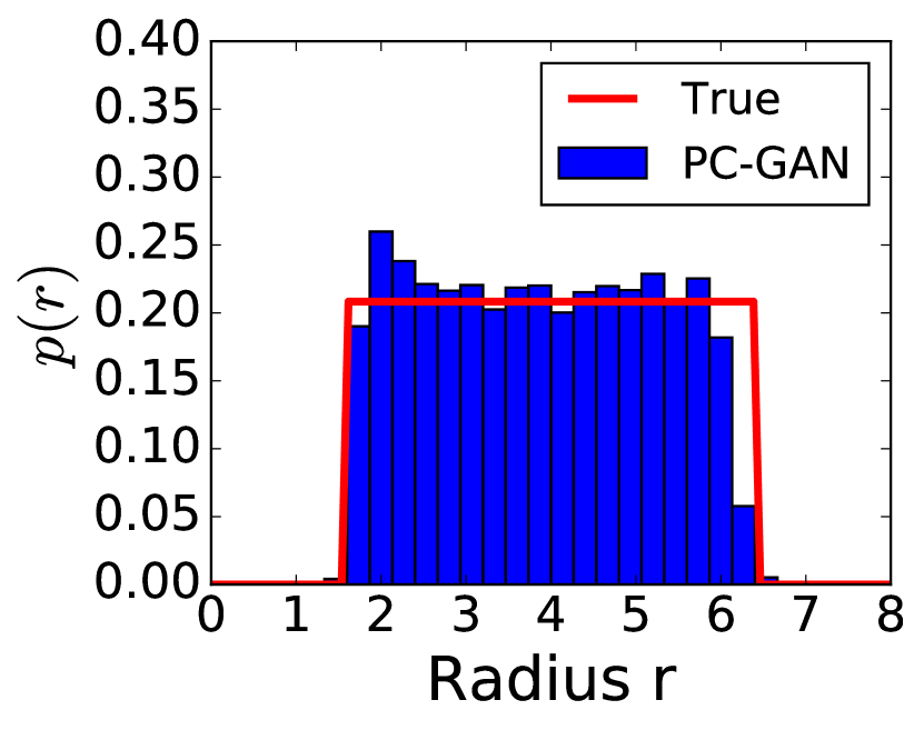
(d) PC-GAN

Figure 5: The reconstructed center and radius distributions. (a) (top) the true center distribution and (bottom) one example of the 2D circle point cloud. (b-d) are the reconstructed center and radius distributions of different algorithms.

From Figure 5, both AAE and PC-GAN can successfully recover the center distribution, but AAE does not learn the radius distribution well. Even if we increase number the hidden layer unit of the decoder to be $20$ (AAE-20), which almost doubles the number of parameters, the performance is still not satisfactory. Compared with AAE, the proposed PC-GAN recovers the both center and radius distributions well with less parameters. The gap of memory usage could be larger if we configure AAE to generate more points, while the model size required for PC-GAN is independent of the number of points. The reason is MLP decoder adopted by Achlioptas et al. (2017) wasted parameters for nearby points. A much larger model (more parameters) can potentially boost the performance, yet would be still restricted to generate a fixed number of points for each object as discussed in Section 5.

6.2 Conditional Generation on ModelNet40

We consider the ModelNet40 (Wu et al., 2015) benchmark, which contains 40 classes of objects. There are $9,843$ training and $2,468$ testing instances. We follow Zaheer et al. (2017) to do pre-processing. For each object, we sampled $10,000$ points from the mesh representation and normalize it to have zero mean (for each axis) and unit (global) variance. During the training, we augment the data by uniformly rotating $0,\pi/8,\dots,7\pi/8$ rad on the $x$-$y$ plane. For PC-GAN, the random noise $z_{2}$ is fixed to be $10$ dimensional for all experiments. For other settings, we follow Achlioptas et al. (2017).

Training on Single Class

We start from a smaller model which is only trained on single class of objects. For AAE, the latent code size for its encoder is $128$ and the decoder outputs $2,048$ points for each object. The number of parameters for encoder and decoder are $15M$ in total. Similarly, we set the size of PC-GAN latent variable (the output of $Q$) to be $128$ dimensional. The number of parameters for $G_{x}$ and $Q$ is less than $1M$ in total.

Training on All Classes.

We also train the proposed model on all $9,843$ objects in the training set. The size of AAE latent code of is increased to be $256$. The number of parameters of its encoder and decoder is $15.2M$. We set the size of PC-GAN latent variable to be $256$ dimensional as well. The number of parameters for $G_{x}$ and $Q$ are around $3M$ in total.

6.2.1 Quantitative Comparison

Table 1: The quantitative results of different models trained on different subsets of ModelNet40 and evaluated on the corresponding testing set. ModelNet10 is a subset containing 10 classes of objects, while ModelNet40 is a full training set. AAE is trained using the code provided by Achlioptas et al. (2017). Three PC-GAN are trained via upper bound $W_{U}$, lower bound $W_{L}$ and sandwiching loss $W_{s}$ discussed in Section 4.

Data	Distance to Face $(\mbox{D2F}\downarrow)$					Coverage $(\uparrow)$
	PC-GAN ($W_{S}$)	AAE	PC-GAN ($W_{U}$)	PC-GAN ($W_{L}$)		PC-GAN ($W_{S}$)	AAE	PC-GAN ($W_{U}$)	PC-GAN ($W_{L}$)
Aeroplanes	1.89E+01	1.99E+01	1.53E+01	2.49E+01		1.95E-01	2.99E-02	1.73E-01	1.88E-01
Benches	1.09E+01	1.41E+01	1.05E+01	2.46E+01		4.44E-01	2.35E-01	2.58E-01	3.83E-01
Cars	4.39E+01	6.23E+01	4.25E+01	6.68E+01		2.35E-01	4.98E-02	1.78E-01	2.35E-01
Chairs	1.01E+01	1.08E+01	1.06E+01	1.08E+01		3.90E-01	1.82E-01	3.57E-01	3.95E-01
Cups	1.44E+03	1.79E+03	1.28E+03	3.01E+03		6.31E-01	3.31E-01	4.32E-01	5.68E-01
Guitars	2.16E+02	1.93E+02	1.97E+02	1.81E+02		2.25E-01	7.98E-02	2.11E-01	2.27E-01
Lamps	1.47E+03	1.60E+03	1.64E+03	2.77E+03		3.89E-01	2.33E-01	3.79E-01	3.66E-01
Laptops	2.43E+00	3.73E+00	2.65E+00	2.58E+00		4.31E-01	2.56E-01	3.93E-01	4.55E-01
Sofa	1.71E+01	1.64E+01	1.45E+01	2.76E+01		3.65E-01	1.62E-01	2.94E-01	3.47E-01
Tables	2.79E+00	2.96E+00	2.44E+00	3.69E+00		3.82E-01	2.59E-01	3.20E-01	3.53E-01
ModelNet10	5.77E+00	6.89E+00	6.03E+00	9.19E+00		3.47E-01	1.90E-01	3.36E-01	3.67E-01
ModelNet40	4.84E+01	5.86E+01	5.24E+01	7.96E+01		3.80E-01	1.85E-01	3.65E-01	3.71E-01

We first evaluate the performance of trained conditional generator $G_{x}$ and the inference network $Q$. We are interested in whether the learned model can model the distribution of the unseen testing data. Therefore, for each testing point cloud, we use $Q$ to infer the latent variable $Q(X)$, then use $G_{x}$ to generate points. We then compare the distribution between the input point cloud and the generated point clouds.

There are many criteria based on finite sample estimation can be used for evaluation, such $f$-divergence and IPM. However, the estimator with finite samples are either biased or with high variance (Peyré et al., 2017; Wang et al., 2009; Póczos et al., 2012; Weed and Bach, 2017). Also, it is impossible to use these estimators with infinitely many samples if they are accessible.

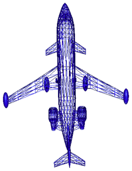
Figure 6: Sample mesh from ModelNet40

For ModelNet40, the meshes of each object are available. In many statistically guaranteed distance estimates, the adopted statistics are commonly based on distance between nearest neighbors (Wang et al., 2009; Póczos et al., 2012). Therefore, we propose to measure the performance with the following criteria. Given a point cloud $\{x_{i}\}_{i=1}^{n}$ and a mesh, which is a collection of faces $\{F_{j}\}_{j=1}^{m}$, we measure the distance to face (D2F) as

$$D2F\left(\{x_{i}\}_{i=1}^{n},\{F_{j}\}_{j=1}^{m}\right)=\frac{1}{n}\sum_{i=1}^{n}\min_{j}\mathcal{D}(x_{i},F_{j}),$$

where $\mathcal{D}(x_{i},F_{j})$ is the Euclidean distance from $x_{i}$ to the face $F_{j}$. This distance is similar to Chamfer distance, which is commonly used for measuring images and point clouds (Achlioptas et al., 2017; Fan et al., 2017), with infinitely samples from true distributions (meshes).

However, the algorithm can have low or zero D2F by only focusing a small portion of the point clouds (mode collapse). Therefore, we are also interested in whether the generated points recover enough supports of the distribution. We compute the Coverage ratio as follows. For each points, we find the its nearest face, we then treat this face is covered. We then compute the ratio of number of faces of a mesh is covered. A sampled mesh is showed in Figure 6, where the details have more faces (non-uniform). Thus, it is difficult to get high coverage for AAE or PC-GAN trained by limited number of sampled points. However, the coverage ratio, on the other hand, serve as an indicator about how much details the model recovers.

The results are reported in Table 1. We compare four different algorithm, AAE and PC-GAN with three objectives, including upper bound $W_{U}$ ( $\epsilon$ approximated Wasserstein distance), lower bound $W_{L}$ (GAN with $L^{2}$ ball constraints and weight clipping), and the sandwiching loss $W_{S}$ as discussed in Section 4.1, The study with $W_{U}$ and $W_{L}$ also serves as the ablation test of the proposed sandwiching loss $W_{s}$.

Comparison between Upper bound, Lower bound and Sandwiching

Since $W_{U}$ directly optimizes distance between training and generated point clouds, $W_{U}$ usually results in smaller D2F than $W_{L}$ in Table 1. One the other hand, although $W_{L}$ only recovers lower bound estimate of Wasserstein distance, its discriminator is known to focus on learning support of the distribution (Bengio, 2018), which results in better coverage (support) than $W_{U}$.

Theoretically, the proposed sandwiching $W_{s}$ results in a tighter Wasserstein distance estimation than $W_{U}$ and $W_{L}$ (Lemma 1). Based on above discussion, it can also be understood as balancing both D2F and coverage by combining both $W_{U}$ and $W_{L}$ to get a desirable middle ground. Empirically, we even observe that $W_{s}$ results in better coverage than $W_{L}$, and competitive D2F with $W_{U}$. The intuitive explanation is that some discriminative tasks are off to $W_{U}$ objective, so the discriminator can focus more on learning distribution supports. We argue that this difference is crucial for capturing the object details. Some reconstructed point clouds of testing data are shown in Figure 7. For aeroplane examples, $W_{U}$ are failed to capture aeroplane tires and $W_{s}$ has better tire than $W_{L}$. For Chair example, $W_{s}$ recovers better legs than $W_{U}$ and better seat cushion than $W_{L}$. Lastly, we highlight $W_{s}$ outperforms others more significantly when training data is larger (ModelNet10 and ModelNet40) in Table 1.

Figure 7: The reconstruction on test objects from seen categories. For each object, from left to right is training data, AAE, and PC-GAN. PC-GAN is better in capturing fine details like wheels of aeroplane or proper chair legs.

Data PC-GAN $(W_{S})$ AAE PC-GAN $(W_{U})$ PC-GAN $(W_{L})$

Comparison between PC-GAN and AAE

In most of cases, PC-GAN with $W_{s}$ has lower D2F in Table 1 with less number of parameters aforementioned. Similar to the argument in Section 6.1, although AAE use larger networks, the decoder wastes parameters for nearby points. AAE only outperforms PC-GAN ($W_{s}$) in Guitar and Sofa in terms of D2F, since the variety of these two classes are low. It is easier for MLP to learn the shared template (basis) of the point clouds. On the other hand, due to the limitation of the fixed number of output points and Chamfer distance objective, AAE has worse coverage than PC-GAN, It can be supported by Figure 7, where AAE is also failed to recover aeroplane tire.

6.3 Hierarchical Sampling

In Section 3, we propose a hierarchical sampling process for sampling point clouds. In the first hierarchy, the generator $G_{\theta}$ samples a object, while the second generator $G_{x}$ samples points to form the point cloud. The randomly sampled results without given any data as input are shown in Figure 8. The point clouds are all smooth, structured and almost symmetric. It shows PC-GAN captures inherent symmetries and patterns in all the randomly sampled objects, even if overall object is not perfectly formed. This highlights that learning point-wise generation scheme encourages learning basic building blocks of objects.

Figure 8: Randomly sampled objects and corresponding point cloud from the hierarchical sampling. Even if there are some defects, the objects are smooth, symmetric and structured. It suggests PC-GAN captures inherent patterns and learns basic building blocks of objects.

6.4 Understand the Learned Manifold

Interpolation

A commonly used method to demonstrate quality of the learned latent space is showing whether the interpolation between two objects on the latent space results in smooth change. We interpolate the inferred representations from two objects by the inference network, and use the generator to sample points. The inter-class result is shown in Figure 9.

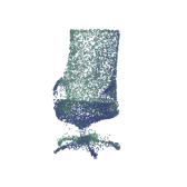
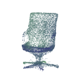
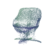
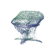
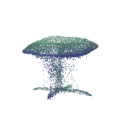
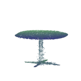
Figure 9: Interpolating between a table and a chair point clouds, using our latent space representation.

It is also popular to show intra-class interpolation. In addition showing simple intra-class interpolations, where the objects are almost aligned, we present an interesting study on interpolations between rotations. During the training, we only rotate data with $8$ possible angles for augmentation, here we show it generalizes to other unseen rotations as shown in Figure 10.

However, if we linearly interpolate the code, the resulted change is scattered and not smooth as shown in Figure 10. Instead of using linear interpolation, We train a 2-layer MLP with limited hidden layer size to be 16, where the input is the angle, output is the corresponding latent representation of rotated object. We then generate the code for rotated planes with this trained MLP. It suggests although the transformation path of rotation on the latent space is not linear, it follows a smooth trajectory. It may also suggest the geodesic path of the learned manifold may not be nearly linear between rotations. Finding the geodesic path with a principal method Shao et al. (2017) and Understanding the geometry of the manifold for point cloud worth more deeper study as future work.

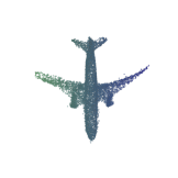
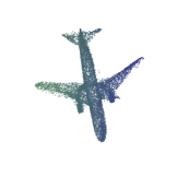
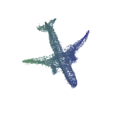
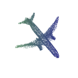
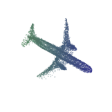
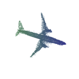
Figure 10: Interpolating between rotation of an aeroplane, using our latent space representation.

Classification

We evaluate the quality of the representation acquired from the learned inference network $Q$. We train the inference network $Q$ and the generator $G_{x}$ on the training split of ModelNet40 with data augmentation as mentioned above for learning generative models without label information. We then extract the latent representation $Q(X)$ for each point clouds and train linear SVM on the that with its label. We apply the same setting to a linear classifier on the latent code of Achlioptas et al. (2017).

We only sample $1000$ as input for our inference network $Q$. As the Deep Sets architecture for the inference network is invariant to number of points, we can sample different number of points as input to the trained inference network for evaluation. Because of the randomness of sampling points for extracting latent representation, we repeat the experiments $20$ times and report the average accuracy and standard deviation on the testing split in Table 2. By using $1000$ points, we are already better than unsupervised algorithms, Achlioptas et al. (2017) with $2048$ points and 3D Voxel GAN (Wu et al., 2016), and competitive with the supervised learning algorithm Deep Sets.

Table 2: Classification accuracy results.

Method	$\#$ points	Accuracy
PC-GAN	1000	$87.5\pm.6\%$
PC-GAN	2048	$87.8\pm.2\%$
AAE (Achlioptas et al., 2017)	2048	$85.5\pm.3\%$
3D GAN (Wu et al., 2016)	voxel	$83.3\%$
Deep Sets (Zaheer et al., 2017)	1000	$87\pm 1\%$
Deep Sets (Zaheer et al., 2017)	5000	$90\pm.3\%$
MVCNN (Su et al., 2015)	images	$90.1\%$
RotationNet (Kanezaki et al., 2018)	images	$97.3\%$

Generalization on Unseen Categories

In above, we studied the reconstruction of unseen testing objects, while PC-GAN still saw the point clouds from the same class during training. Here we study a more challenging task. We train PC-GAN on first 30 (Alphabetic order) class, and test on the other fully unseen 10 classes. Some reconstructed (conditionally generated) point clouds are shown in Figure 11. More (larger) results can be found in Appendix LABEL:sec:larger. For the object from the unseen classes, the conditionally generated point clouds still recovers main shape and reasonable geometry structure, which confirms the advantage of the proposed PC-GAN: by enforcing the point-wise transformation, the model is forced to learn the underlying geometry structure and the shared building blocks, instead of naively copying the input from the conditioning. The resulted D2F and coverage are $57.4$ and $0.36$, which are only slightly worse than $48.4$ and $0.38$ by training on whole 40 classes in Table 1 (ModelNet40), which also supports the claims of the good generalization ability of PC-GAN.

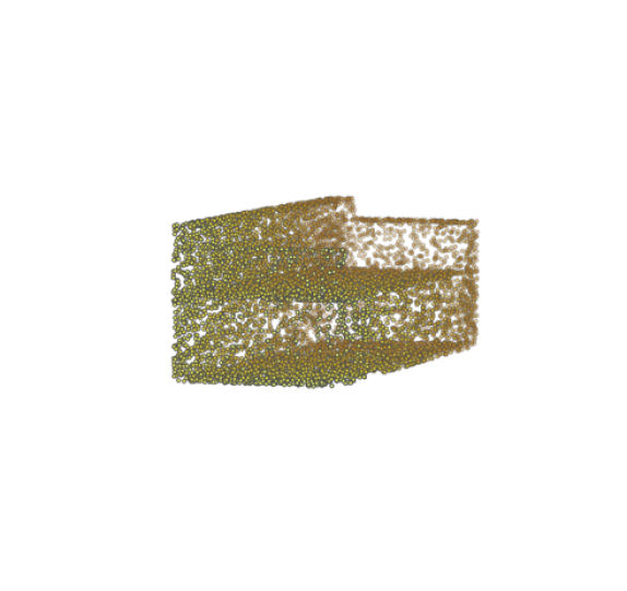
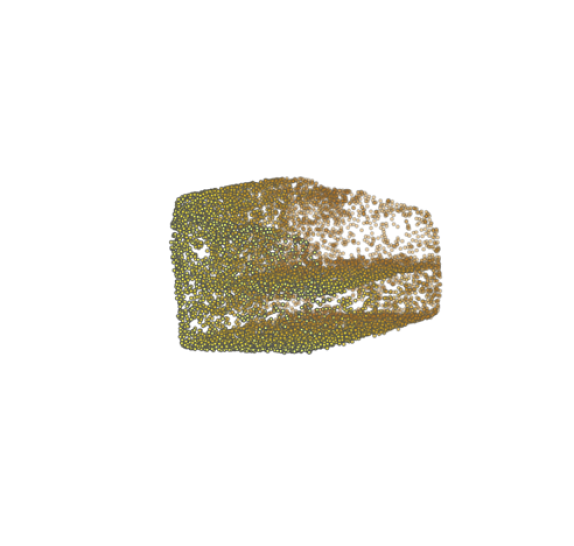
(a) Sofa

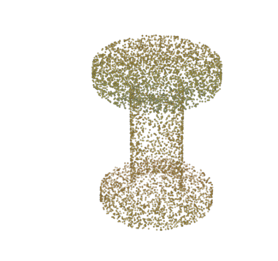
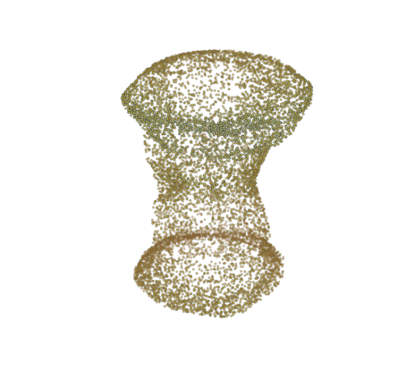
(b) Stool

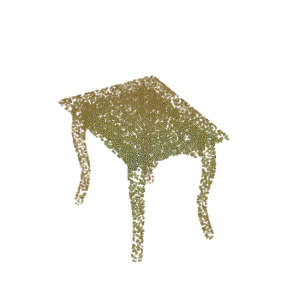
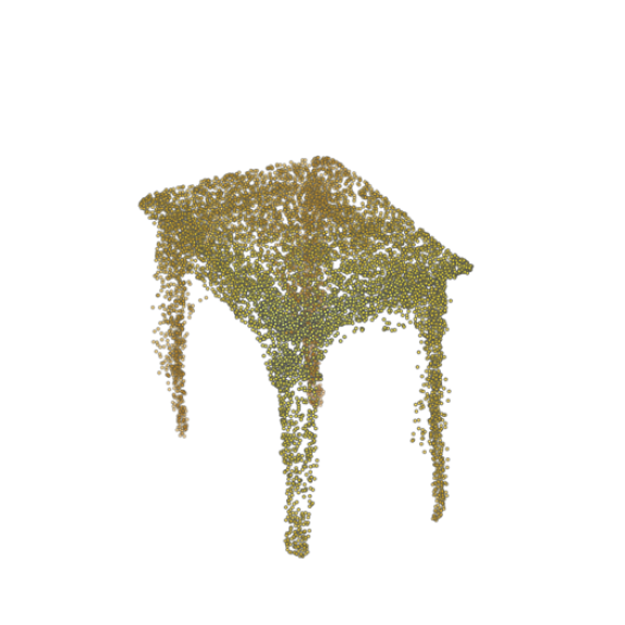
(c) Table

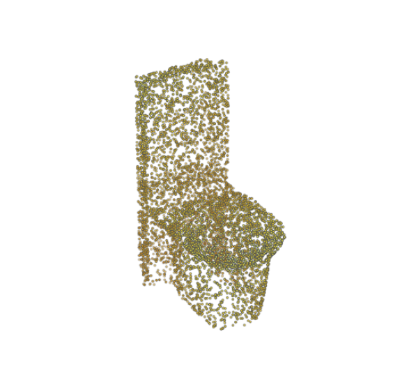
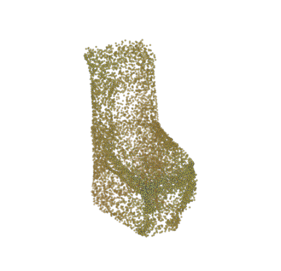
(d) Toilet

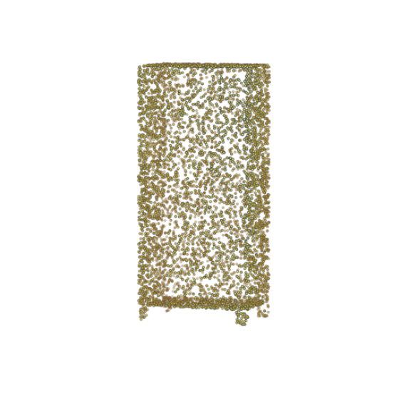
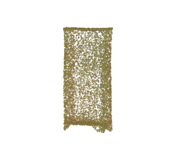
(e) TV Stand

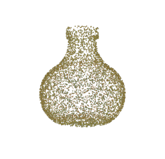
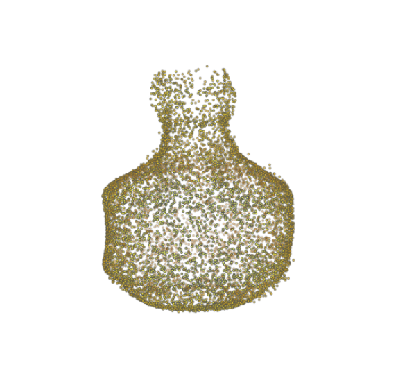
(f) Vase

Figure 11: The reconstructed objects from unseen categories. In each plot, LHS is true data while RHS is PC-GAN. PC-GAN generalizes well as it can match patterns and symmetries from categories seen in the past to new unseen categories.

6.5 Images to Point Cloud

Here we demonstrate a potential extension of the proposed PC-GAN for images to point cloud applications. After training $Q$ as described in 6.3, instead of learning $G_{\theta}$ for hierarchical sampling, we train a regressor $R$, where the input is the different views of the point cloud $X$, and the output is $Q(X)$. In this proof of concept experiment, we use the $12$ view data and the Res18 architecture in Su et al. (2015), while we change the output size to be $256$. Some example results on reconstructing testing data is shown in Figure 12. A straightforward extension is using end-to-end training instead of two-staged approached adopted here. Also, after aligning objects and take representative view along with traditional ICP techniques, we can also do single view to point cloud transformation as Choy et al. (2016); Fan et al. (2017); Häne et al. (2017); Groueix et al. (2018a), which is not the main focus of this paper and we leave it for future work.

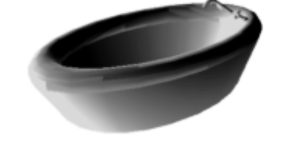
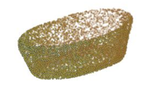
(a) Lamp

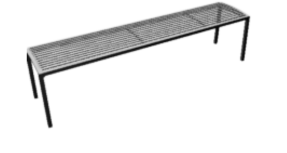
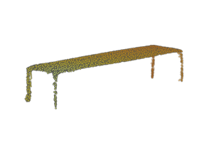
(b) Chair

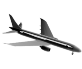
(c) Plane

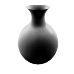
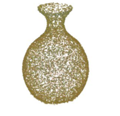
(d) Vase

Figure 12: Images to Point Clouds.

7 Conclusion

In this paper, we first showed a straightforward extension of existing GAN algorithm is not applicable to point clouds. We then proposed a GAN modification (PC-GAN) that is capable of learning to generate point clouds by using ideas both from hierarchical Bayesian modeling and implicit generative models. We further propose a sandwiching objective which results in a tighter Wasserstein distance estimate theoretically and better performance empirically.

In contrast to some existing methods (Achlioptas et al., 2017), PC-GAN can generate arbitrary as many i.i.d. points as we need to form a point clouds without pre-specification. Quantitatively, PC-GAN achieves competitive or better results using smaller network than existing methods. We also demonstrated that PC-GAN can capture delicate details of point clouds and generalize well even on unseen data. Our method learns “point-wise” transformations which encourage the model to learn the building components of the objects, instead of just naively copying the whole object. We also demonstrate other interesting results, including point cloud interpolation and image to point clouds.

Although we only focused on 3D applications in this paper, our framework can be naturally generalized to higher dimensions. In the future we would like to explore higher dimensional applications, where each 3D point can have other attributes, such as RGB colors and 3D velocity vectors.

Appendix A Technical Proof

Lemma 1.

Suppose we have two approximators to Wasserstein distance: an upper bound $W_{U}$ and a lower $W_{L}$, such that $\forall P,G:(1+\epsilon_{1})w(\mathbb{P},\mathbb{G})\leq W_{U}(\mathbb{P},\mathbb{G})\leq(1+\epsilon_{2})w(\mathbb{P},\mathbb{G})$ and $\forall P,G:(1-\epsilon_{2})w(\mathbb{P},\mathbb{G})\leq W_{L}(\mathbb{P},\mathbb{G})\leq(1-\epsilon 1)w(\mathbb{P},\mathbb{G})$ respectively, for some $\epsilon_{2}>\epsilon_{1}>0$ and $\epsilon_{1}>\epsilon_{2}/3$. Then, using the sandwiched estimator $W_{\lambda}$ from (6), we can achieve tighter estimate of the Wasserstein distance than using either one estimator, i.e.

$$\exists\lambda:|W_{\lambda}(\mathbb{P},\mathbb{G})-w(\mathbb{P},\mathbb{G})|<\min\{|W_{U}(\mathbb{P},\mathbb{G})-w(\mathbb{P},\mathbb{G})|,|W_{L}(\mathbb{P},\mathbb{G})-w(\mathbb{P},\mathbb{G})|\}$$ (12)

Proof.

We prove the claim by show that LHS is at most $\epsilon_{1}$, which is the lower bound for RHS.

$$|W_{\lambda} (\mathbb{P},\mathbb{G})-w(\mathbb{P},\mathbb{G})|$$ (13)

$$=|(1-\lambda)W_{U}(\mathbb{P},\mathbb{G})+\lambda W_{L}(\mathbb{P},\mathbb{G})-w(\mathbb{P},\mathbb{G})|$$

$$=|(1-\lambda)(W_{U}(\mathbb{P},\mathbb{G})-w(\mathbb{P},\mathbb{G}))-\lambda(w(\mathbb{P},\mathbb{G})-W_{L}(\mathbb{P},\mathbb{G}))|$$

$$\leq\max\{(1-\lambda)\underbrace{(W_{U}(\mathbb{P},\mathbb{G})-w(\mathbb{P},\mathbb{G}))}_{\leq\epsilon_{2}},\lambda\underbrace{(w(\mathbb{P},\mathbb{G})-W_{L}(\mathbb{P},\mathbb{G}))}_{\leq\epsilon_{2}}\}$$

$$\qquad\qquad-\min\{(1-\lambda)\underbrace{(W_{U}(\mathbb{P},\mathbb{G})-w(\mathbb{P},\mathbb{G}))}_{\geq\epsilon_{1}},\lambda\underbrace{(w(\mathbb{P},\mathbb{G})-W_{L}(\mathbb{P},\mathbb{G}))}_{\geq\epsilon_{1}}\}$$

$$\leq\max\{(1-\lambda),\lambda\}\epsilon_{2}-\min\{(1-\lambda),\lambda\}\epsilon_{1}$$

Without loss of generality we can assume $\lambda<0.5$, which brings us to

$$|W_{\lambda}(\mathbb{P},\mathbb{G})-w(\mathbb{P},\mathbb{G})|\leq(1-\lambda)\epsilon_{2}-\lambda\epsilon_{1}$$ (14)

Now if we chose $\frac{\epsilon_{2}-\epsilon_{1}}{\epsilon_{2}+\epsilon_{1}}<\lambda<0.5$, then $|W_{\lambda}(\mathbb{P},\mathbb{G})-w(\mathbb{P},\mathbb{G})|<\epsilon_{1}$ as desired. ∎

Lemma 2.

There exists $k>0$ such that

$$\max_{f\in\Omega_{c}\cap\Omega_{\phi}}\mathbb{E}_{x\sim P}[f_{\phi}(x)]-\mathbb{E}_{x\sim G}[f_{\phi}(x)]\leq\frac{1}{k}w(\mathbb{P},\mathbb{G})$$ (15)

Proof.

Since there exists $k$ such that $\max_{f\in\Omega_{c}}\mathbb{E}_{x\sim P}[f_{\phi}(x)]-\mathbb{E}_{x\sim G}[f_{\phi}(x)]\leq\frac{1}{k}w(\mathbb{P},\mathbb{G})$, it is clear that

$$\max_{f\in\Omega_{c}\cap\Omega_{\phi}}\mathbb{E}_{x\sim P}[f_{\phi}(x)]-\mathbb{E}_{x\sim G}[f_{\phi}(x)]\leq\max_{f\in\Omega_{c}}\mathbb{E}_{x\sim P}[f_{\phi}(x)]-\mathbb{E}_{x\sim G}[f_{\phi}(x)]\leq\frac{1}{k}w(\mathbb{P},\mathbb{G}).$$ (16)

∎

Appendix B Permutation Equivariance Layers

We briefly review the notion of Permutation Equivariance Layers proposed by Zaheer et al. (2017) as a background required for this paper. For more details, please refer to Zaheer et al. (2017).

Zaheer et al. (2017) propose a generic framework of deep learning for set data. The building block which can be stacked to be deep neural networks is called Permutation Equivariance Layer. One Permutation Equivariance Layer example is defined as

$$f(x_{i})=\sigma(x_{i}+\gamma\mbox{maxpool}(X)),$$

where $\sigma$ can be any functions (e.g. parametrized by neural networks) and $X={x_{1},\dots,x_{n}}$ is an input set. Also, the mox pooling operation can be replaced with mean pooling. We note that PointNetQi et al. (2017a) is a special case of using Permutation Equivariance Layer by properly defining $\sigma(\cdot)$. In our experiments, we follow Zaheer et al. (2017) to set $\sigma$ to be a linear layer with output size $h$ followed by any nonlinear activation function.

Appendix C Experiment Settings

C.1 Synthetic Data

The batch size is fixed to be $64$. We sampled 10,000 samples for training and testing.

For the inference network, we stack $3$ mean Permutation Equivariance Layer (Zaheer et al., 2017), where the hidden layer size (the output of the first two layers ) is $30$ and the final output size is $15$. The activation function are used SoftPlus. For the generater is a $5$ layer MLP, where the hidden layer size is set to be $30$. The discirminator is $4$ layer MLP with hidden layer size to be $30$. For  Achlioptas et al. (2017), we change their implementation by replcing the number of filters for encoder to be $[30,30,30,30,15]$, while the hidden layer width for decoder is $10$ or $20$ except for the output layer. The decoder is increased from 3 to 4 layers to have more capacity.

C.2 ModelNet40

We follow Zaheer et al. (2017) to do pre-processing. For each object, we sampled $10,000$ points from the mesh representation and normalize it to have zero mean (for each axis) and unit (global) variance. During the training, we augment the data by uniformly rotating $0,\pi/8,\dots,7\pi/8$ rad on the $x$-$y$ plane. The random noise $z_{2}$ of PC-GAN is fixed to be $10$ dimensional for all experiments.

For $Q$ of single class model, we stack $3$ max Permutation Equivariance Layer with output size to be $128$ for every layer. On the top of the satck, we have a $2$ layer MLP with the same width and the output . The generator $G_{x}$ is a $4$ layer MLP where the hidden layer size is $128$ and output size is $3$. The discirminator is $4$ layer MLP with hidden layer size to be $128$.

For training whole ModelNet40 training set, we increae the width to be $256$. The generator $G_{x}$ is a $5$ layer MLP where the hidden layer size is $256$ and output size is $3$. The discirminator is $5$ layer MLP with hidden layer size to be $256$. For hirarchical sampling, the top generator $G_{\theta}$ and discriminator are all $5$-layer MLP with hidden layer size to be $256$.

For AAE, we follow every setting used in  Achlioptas et al. (2017), where the latent code size is $128$ and $256$ for single class model and whole ModelNet40 models.

References

- Achlioptas et al. (2017) Panos Achlioptas, Olga Diamanti, Ioannis Mitliagkas, and Leonidas Guibas. Learning representations and generative models for 3d point clouds. arXiv preprint arXiv:1707.02392, 2017.
- Arjovsky et al. (2017) Martin Arjovsky, Soumith Chintala, and Léon Bottou. Wasserstein gan. ICML, 2017.
- Arora et al. (2017) Sanjeev Arora, Rong Ge, Yingyu Liang, Tengyu Ma, and Yi Zhang. Generalization and equilibrium in generative adversarial nets (gans). arXiv preprint arXiv:1703.00573, 2017.
- Bengio (2018) Yoshua Bengio. Gans and unsupervised representation learning, 2018.
- Bertsekas (1985) Dimitri P Bertsekas. A distributed asynchronous relaxation algorithm for the assignment problem. In Decision and Control, 1985.
- Bishop (2006) M Christopher Bishop. Pattern Recognition and Machine Learning. Springer-Verlag New York, 2006.
- Bronstein et al. (2017) Michael M Bronstein, Joan Bruna, Yann LeCun, Arthur Szlam, and Pierre Vandergheynst. Geometric deep learning: going beyond euclidean data. IEEE Signal Processing Magazine, 2017.
- Chang et al. (2017) JH Rick Chang, Chun-Liang Li, Barnabas Poczos, BVK Vijaya Kumar, and Aswin C Sankaranarayanan. One network to solve them all—solving linear inverse problems using deep projection models. arXiv preprint, 2017.
- Choy et al. (2016) Christopher B Choy, Danfei Xu, JunYoung Gwak, Kevin Chen, and Silvio Savarese. 3d-r2n2: A unified approach for single and multi-view 3d object reconstruction. In ECCV, 2016.
- Cuturi (2013) Marco Cuturi. Sinkhorn distances: Lightspeed computation of optimal transport. In NIPS, 2013.
- Dai et al. (2017) Bo Dai, Sanja Fidler, Raquel Urtasun, and Dahua Lin. Towards diverse and natural image descriptions via a conditional gan. arXiv preprint arXiv:1703.06029, 2017.
- Dumoulin et al. (2016) Vincent Dumoulin, Ishmael Belghazi, Ben Poole, Olivier Mastropietro, Alex Lamb, Martin Arjovsky, and Aaron Courville. Adversarially learned inference. arXiv preprint arXiv:1606.00704, 2016.
- Eckart et al. (2015) Ben Eckart, Kihwan Kim, Alejandro Troccoli, Alonzo Kelly, and Jan Kautz. Mlmd: Maximum likelihood mixture decoupling for fast and accurate point cloud registration. In 3DV, 2015.
- Engel et al. (2017) Jesse Engel, Matthew Hoffman, and Adam Roberts. Latent constraints: Learning to generate conditionally from unconditional generative models. arXiv preprint arXiv:1711.05772, 2017.
- Fan et al. (2017) Haoqiang Fan, Hao Su, and Leonidas J Guibas. A point set generation network for 3d object reconstruction from a single image. In CVPR, 2017.
- Genevay et al. (2018) Aude Genevay, Gabriel Peyré, and Marco Cuturi. Learning generative models with sinkhorn divergences. In AISTATS, 2018.
- Goodfellow et al. (2014) Ian Goodfellow, Jean Pouget-Abadie, Mehdi Mirza, Bing Xu, David Warde-Farley, Sherjil Ozair, Aaron Courville, and Yoshua Bengio. Generative adversarial nets. In NIPS, 2014.
- Groueix et al. (2018a) Thibault Groueix, Matthew Fisher, Vladimir G Kim, Bryan C Russell, and Mathieu Aubry. Atlasnet: A papier-m^ ach’e approach to learning 3d surface generation. arXiv preprint arXiv:1802.05384, 2018a.
- Groueix et al. (2018b) Thibault Groueix, Matthew Fisher, Vladimir G Kim, Bryan C Russell, and Mathieu Aubry. A papier-mâché approach to learning 3d surface generation. In CVPR, 2018b.
- Gulrajani et al. (2017) Ishaan Gulrajani, Faruk Ahmed, Martin Arjovsky, Vincent Dumoulin, and Aaron Courville. Improved training of wasserstein gans. In NIPS, 2017.
- Häne et al. (2017) Christian Häne, Shubham Tulsiani, and Jitendra Malik. Hierarchical surface prediction for 3d object reconstruction. In 3D Vision (3DV), 2017 International Conference on, 2017.
- Hjelm et al. (2017) R. Devon Hjelm, Athul Paul Jacob, Tong Che, Kyunghyun Cho, and Yoshua Bengio. Boundary-seeking generative adversarial networks. arXiv:1702.08431, 2017.
- Isola et al. (2017) Phillip Isola, Jun-Yan Zhu, Tinghui Zhou, and Alexei A Efros. Image-to-image translation with conditional adversarial networks. arXiv preprint, 2017.
- Jian and Vemuri (2005) Bing Jian and Baba C Vemuri. A robust algorithm for point set registration using mixture of gaussians. In ICCV, 2005.
- Kalogerakis et al. (2017) Evangelos Kalogerakis, Melinos Averkiou, Subhransu Maji, and Siddhartha Chaudhuri. 3d shape segmentation with projective convolutional networks. CVPR, 2, 2017.
- Kanezaki et al. (2018) Asako Kanezaki, Yasuyuki Matsushita, and Yoshifumi Nishida. Rotationnet: Joint object categorization and pose estimation using multiviews from unsupervised viewpoints. In CVPR, 2018.
- Kang (2017) Eunsu Kang. FACE Exhibition, 2017. Judith Rae Solomon Gallery, Youngstown, OH. http://art.ysu.edu/2017/09/06/face-by-eunsu-kang-and-collaborators/.
- Karras et al. (2017) Tero Karras, Timo Aila, Samuli Laine, and Jaakko Lehtinen. Progressive growing of gans for improved quality, stability, and variation. arXiv preprint arXiv:1710.10196, 2017.
- Kim et al. (2017) Yoon Kim, Kelly Zhang, Alexander M Rush, Yann LeCun, et al. Adversarially regularized autoencoders for generating discrete structures. arXiv preprint arXiv:1706.04223, 2017.
- Kingma and Welling (2013) Diederik P Kingma and Max Welling. Auto-encoding variational bayes. arXiv preprint arXiv:1312.6114, 2013.
- Lamb et al. (2016) Alex M Lamb, Anirudh Goyal ALIAS PARTH GOYAL, Ying Zhang, Saizheng Zhang, Aaron C Courville, and Yoshua Bengio. Professor forcing: A new algorithm for training recurrent networks. In NIPS, 2016.
- Li et al. (2018) Chongxuan Li, Max Welling, Jun Zhu, and Bo Zhang. Graphical generative adversarial networks. arXiv preprint arXiv:1804.03429, 2018.
- Li et al. (2017a) Chun-Liang Li, Wei-Cheng Chang, Yu Cheng, Yiming Yang, and Barnabás Póczos. Mmd gan: Towards deeper understanding of moment matching network. In NIPS, 2017a.
- Li et al. (2017b) Chunyuan Li, Hao Liu, Changyou Chen, Yuchen Pu, Liqun Chen, Ricardo Henao, and Lawrence Carin. Alice: Towards understanding adversarial learning for joint distribution matching. In NIPS, 2017b.
- Makhzani et al. (2015) Alireza Makhzani, Jonathon Shlens, Navdeep Jaitly, Ian Goodfellow, and Brendan Frey. Adversarial autoencoders. arXiv preprint arXiv:1511.05644, 2015.
- Mao et al. (2017) Xudong Mao, Qing Li, Haoran Xie, Raymond YK Lau, and Zhen Wang. Least squares generative adversarial networks. In ICCV, 2017.
- Maturana and Scherer (2015) Daniel Maturana and Sebastian Scherer. Voxnet: A 3d convolutional neural network for real-time object recognition. In IROS, 2015.
- Mirza and Osindero (2014) Mehdi Mirza and Simon Osindero. Conditional generative adversarial nets. arXiv preprint arXiv:1411.1784, 2014.
- Mroueh and Sercu (2017) Youssef Mroueh and Tom Sercu. Fisher gan. In NIPS, 2017.
- Mroueh et al. (2017) Youssef Mroueh, Chun-Liang Li, Tom Sercu, Anant Raj, and Yu Cheng. Sobolev gan. arXiv preprint arXiv:1711.04894, 2017.
- Nowozin et al. (2016) Sebastian Nowozin, Botond Cseke, and Ryota Tomioka. f-gan: Training generative neural samplers using variational divergence minimization. In NIPS, 2016.
- Oliva et al. (2018) Junier B Oliva, Avinava Dubey, Barnabás Póczos, Jeff Schneider, and Eric P Xing. Transformation autoregressive networks. arXiv preprint arXiv:1801.09819, 2018.
- Oord et al. (2016) Aaron van den Oord, Nal Kalchbrenner, and Koray Kavukcuoglu. Pixel recurrent neural networks. arXiv preprint arXiv:1601.06759, 2016.
- Pathak et al. (2016) Deepak Pathak, Philipp Krahenbuhl, Jeff Donahue, Trevor Darrell, and Alexei A Efros. Context encoders: Feature learning by inpainting. In CVPR, 2016.
- Peyré et al. (2017) Gabriel Peyré, Marco Cuturi, et al. Computational optimal transport. Technical report, 2017.
- Póczos et al. (2012) Barnabás Póczos, Liang Xiong, and Jeff Schneider. Nonparametric divergence estimation with applications to machine learning on distributions. arXiv preprint arXiv:1202.3758, 2012.
- Qi et al. (2016) Charles R Qi, Hao Su, Matthias Nießner, Angela Dai, Mengyuan Yan, and Leonidas J Guibas. Volumetric and multi-view cnns for object classification on 3d data. In CVPR, 2016.
- Qi et al. (2017a) Charles R Qi, Hao Su, Kaichun Mo, and Leonidas J Guibas. Pointnet: Deep learning on point sets for 3d classification and segmentation. CVPR, 2017a.
- Qi et al. (2017b) Charles Ruizhongtai Qi, Li Yi, Hao Su, and Leonidas J Guibas. Pointnet++: Deep hierarchical feature learning on point sets in a metric space. In NIPS, 2017b.
- Salimans et al. (2016) Tim Salimans, Ian Goodfellow, Wojciech Zaremba, Vicki Cheung, Alec Radford, and Xi Chen. Improved techniques for training gans. In NIPS, 2016.
- Shao et al. (2017) Hang Shao, Abhishek Kumar, and P Thomas Fletcher. The riemannian geometry of deep generative models. arXiv preprint arXiv:1711.08014, 2017.
- Strom et al. (2010) Johannes Strom, Andrew Richardson, and Edwin Olson. Graph-based segmentation for colored 3d laser point clouds. In IROS, 2010.
- Su et al. (2015) Hang Su, Subhransu Maji, Evangelos Kalogerakis, and Erik Learned-Miller. Multi-view convolutional neural networks for 3d shape recognition. In ICCV, 2015.
- Tatarchenko et al. (2017) Maxim Tatarchenko, Alexey Dosovitskiy, and Thomas Brox. Octree generating networks: Efficient convolutional architectures for high-resolution 3d outputs. In ICCV, 2017.
- Tolstikhin et al. (2017) Ilya Tolstikhin, Olivier Bousquet, Sylvain Gelly, and Bernhard Schoelkopf. Wasserstein auto-encoders. arXiv preprint arXiv:1711.01558, 2017.
- Vondrick et al. (2016) Carl Vondrick, Hamed Pirsiavash, and Antonio Torralba. Generating videos with scene dynamics. In NIPS, pages 613–621, 2016.
- Wang et al. (2009) Qing Wang, Sanjeev R Kulkarni, and Sergio Verdú. Divergence estimation for multidimensional densities via -nearest-neighbor distances. IEEE Transactions on Information Theory, 2009.
- Wang and Gupta (2016) Xiaolong Wang and Abhinav Gupta. Generative image modeling using style and structure adversarial networks. In ECCV, 2016.
- Wang et al. (2018) Yue Wang, Yongbin Sun, Ziwei Liu, Sanjay E Sarma, Michael M Bronstein, and Justin M Solomon. Dynamic graph cnn for learning on point clouds. arXiv preprint arXiv:1801.07829, 2018.
- Weed and Bach (2017) Jonathan Weed and Francis Bach. Sharp asymptotic and finite-sample rates of convergence of empirical measures in wasserstein distance. arXiv preprint arXiv:1707.00087, 2017.
- Wu et al. (2016) Jiajun Wu, Chengkai Zhang, Tianfan Xue, Bill Freeman, and Josh Tenenbaum. Learning a probabilistic latent space of object shapes via 3d generative-adversarial modeling. In NIPS, 2016.
- Wu et al. (2015) Zhirong Wu, Shuran Song, Aditya Khosla, Fisher Yu, Linguang Zhang, Xiaoou Tang, and Jianxiong Xiao. 3d shapenets: A deep representation for volumetric shapes. In CVPR, 2015.
- Yang et al. (2018) Yaoqing Yang, Chen Feng, Yiru Shen, and Dong Tian. Foldingnet: Point cloud auto-encoder via deep grid deformation. In CVPR, volume 3, 2018.
- Yu et al. (2016) Lantao Yu, Weinan Zhang, Jun Wang, and Yong Yu. Seqgan: Sequence generative adversarial nets with policy gradient. CoRR, abs/1609.05473, 2016.
- Zaheer et al. (2017) Manzil Zaheer, Satwik Kottur, Siamak Ravanbakhsh, Barnabas Poczos, Ruslan R Salakhutdinov, and Alexander J Smola. Deep sets. In NIPS, 2017.
- Zhao et al. (2016) Junbo Zhao, Michael Mathieu, and Yann LeCun. Energy-based generative adversarial network. arXiv preprint arXiv:1609.03126, 2016.
- Zhu et al. (2017) Jun-Yan Zhu, Taesung Park, Phillip Isola, and Alexei A Efros. Unpaired image-to-image translation using cycle-consistent adversarial networks. arXiv preprint arXiv:1703.10593, 2017.