UT-18-21

Flavon Stabilization in Models with
Discrete Flavor Symmetry

So Chigusa^(a), Shinta Kasuya^(b) and Kazunori Nakayama^(a,c)

^(a)Department of Physics, Faculty of Science,
The University of Tokyo, Bunkyo-ku, Tokyo 113-0033, Japan
^(b)Department of Mathematics and Physics,
Kanagawa University, Kanagawa 259-1293, Japan
^(c)Kavli Institute for the Physics and Mathematics of the Universe (WPI),
The University of Tokyo, Kashiwa, Chiba 277-8583, Japan

We propose a simple mechanism for stabilizing flavon fields with aligned vacuum structure in models with discrete flavor symmetry. The basic idea is that flavons are stabilized by the balance between the negative soft mass and non-renormalizable terms in the potential. We explicitly discuss how our mechanism works in $A_{4}$ flavor model, and show that the field content is significantly simplified. It also works as a natural solution to the cosmological domain wall problem.

1 Introduction

There are many proposals that try to explain the observed pattern of neutrino masses and mixings using discrete flavor symmetry (for reviews, see Refs. [1, 2, 3, 4]). In these classes of models, the Lagrangian is assumed to be invariant under some discrete symmetry and charged leptons and neutrinos obtain masses through vacuum expectation values (VEVs) of scalar fields which are charged under the discrete symmetry, called flavons. Thus the discrete symmetry is spontaneously broken by the VEVs of flavons.

Models with the spontaneous breakdown of discrete symmetry necessarily have several discrete degenerate vacua. In general, such a model suffers from the cosmological domain wall problem [5]. Domain wall problem in the context of discrete flavor symmetry has been discussed in a few papers [6, 7, 8, 9]. Ref. [6] considered some possibilities that may avoid the domain wall problem in the $A_{4}$ model based on the scalar potential proposed in Ref. [10]. The inflation scale could be lower than the flavor symmetry breaking scale so that the flavor symmetry breaking occurs before inflation, but there is a flat direction in the scalar potential in the model of Ref. [10], and hence this solution does not work unless the inflation scale is lower than the soft supersymmetry (SUSY) breaking scale. One possibility is that (a part of) the discrete symmetry is explicitly broken so that the VEV of flat direction does not produce exactly stable domain walls.Ref. [6] also briefly discussed a possibility that the flat direction in the scalar potential obtains a large field value during/after inflation due to the Hubble mass correction, so that domain walls are inflated away. However, we find out that actually it is difficult to stabilize the flat direction in the desired way as far as we work with the scalar sector of Ref. [10], because the flat direction necessarily has unwanted higher dimensional operators that is not suitable for the purpose of solving the domain wall problem.

In this paper, we propose a very simple alternative mechanism to stabilize the flavon potential with desired alignment structure. In our model, flavons are stabilized by the balance between the negative soft SUSY breaking mass and non-renormalizable terms in the potential. The field content is then significantly simplified, and we do not need any additional field (so-called driving field). In addition, the cosmological domain wall problem is naturally solved independent of the inflation scale.

The structure of the paper is as follows. In the next section, we first review $A_{4}$ model briefly. In Sec. 3, we explain the basic idea of our novel mechanism of the flavon stabilization and study a concrete model with $A_{4}$ symmetry in Sec. 4. We show how the domain wall problem is naturally avoided in our model in Sec. 5. Sec. 6 is devoted to our conclusions and discussion. $A_{4}$ representations are summarized in the Appendix.

2 Brief description of $A_{4}$ model

We assume the superpotential of the form

$$W=W_{\ell}+W_{\rm f},$$ (1)

where $W_{\rm f}$ is related to the stabilization of the flavon fields discussed in the next section, and $W_{\ell}$ is given by [10]

$$W_{\ell} =\frac{y_{e}}{\Lambda}e^{c}H_{d}(\varphi_{T}\ell)+\frac{y_{\mu}}{\Lambda}\mu^{c}H_{d}(\varphi_{T}\ell)^{\prime}+\frac{y_{\tau}}{\Lambda}\tau^{c}H_{d}(\varphi_{T}\ell)^{\prime\prime}$$

$$\quad+\frac{x_{a}}{\Lambda^{2}}H_{u}H_{u}\xi(\ell\ell)+\frac{x_{b}}{\Lambda^{2}}H_{u}H_{u}(\varphi_{S}\ell\ell)+\cdots,$$ (2)

where $\ell$ denotes the $A_{4}$ triplet lepton doublets, while $A_{4}$ singlets $e^{c},\mu^{c},\tau^{c},H_{u}$, and $H_{d}$ represent the right-handed electron, muon, tau, the up-type Higgs, and the down-type Higgs, respectively. Also, $\varphi_{T}$, $\varphi_{S}$, and $\xi$ are flavon fields and $\Lambda$ is the cutoff scale. We assign the charges of the fields under the $A_{4}$ symmetry as in Ref. [10] (see Table 1). Here $(\cdots)$, $(\cdots)^{\prime}$, and $(\cdots)^{\prime\prime}$ represent the contraction of various 3 representations that transform respectively as 1, $\textbf{1}^{\prime}$, and $\textbf{1}^{\prime\prime}$. In addition, the dots in Eq. (2) stand for the higher dimensional operators. In this paper, we take a basis of the triplet representation that diagonalizes generators of the subgroup $Z_{3}\subset A_{4}$. For details of the convention of the basis and the product of representations, see Appendix A.

If the flavon fields obtain VEVs of the following structure,

$$\left<\varphi_{T}\right>=(v_{T},0,0),~{}~{}~{}\left<\varphi_{S}\right>=(v_{S},v_{S},v_{S}),~{}~{}~{}\left<\xi\right>=v_{\xi},$$ (3)

the diagonal mass matrix of the charged lepton is obtained, while the neutrino mixing matrix becomes the so-called tri-bimaximal form [12, 11, 10]. Here and below, we use the same notation $\varphi_{T}$, $\varphi_{S}$, and $\xi$ for the scalar component of the corresponding superfield. The recent neutrino oscillation data requires deviation from the tri-bimaximal form. Extensions of the $A_{4}$ model to account for the observed data are found, e.g. in Refs. [13, 14]. For a while, however, we study this minimal setup to avoid unnecessary complexity and discuss modification related to the deviation from the tri-bimaximal structure in Sec. 4.4.

3 Basic idea for the novel simple flavon stabilization

	$\ell$	$e^{c}$	$\mu^{c}$	$\tau^{c}$	$H_{u}$	$H_{d}$	$\varphi_{T}$	$\varphi_{S}$	$\xi$
$A_{4}$	${\bf 3}$	${\bf 1}$	${\bf 1^{\prime\prime}}$	${\bf 1^{\prime}}$	${\bf 1}$	${\bf 1}$	${\bf 3}$	${\bf 3}$	${\bf 1}$
$Z_{12}$	$\rho^{5}$	$\rho^{7}$	$\rho^{7}$	$\rho^{7}$	$1$	$1$	$1$	$\rho^{2}$	$\rho^{2}$
U(1)R	$\frac{5}{6}$	$\frac{5}{6}$	$\frac{5}{6}$	$\frac{5}{6}$	0	0	$\frac{1}{3}$	$\frac{1}{3}$	$\frac{1}{3}$

Table 1: Charge assignments under $A_{4}$, $Z_{12}$ and U(1)_R for leptons and various Higgs and flavon fields. Here $\rho\equiv e^{\pi i/6}$ is an element of $Z_{12}$ rotation.

In the most known models so far, the flavon fields are stabilized at the renormalizable level. Then we need to introduce several driving fields in addition to the flavon fields in order to obtain the alignment structure of Eq. (3), and the resulting superpotential is complicated [10]. Moreover, there may remain a flat direction in the scalar potential that requires additional stabilization mechanism and it makes domain wall problem serious.

We propose a simple superpotential that successfully realize the alignment structure of Eq. (3). The basic idea is that the flavon fields are stabilized by the balance between the negative soft SUSY breaking mass and non-renormalizable terms in the potential. Schematically, we just assume

$$W_{\rm f}=\frac{\varphi^{n}}{n\Lambda^{n-3}},$$ (4)

where $\varphi$ collectively denotes the flavon fields. Giving the tachyonic soft SUSY breaking mass term as $V_{\rm SB}=-m_{\varphi}^{2}|\varphi|^{2}$, we can stabilize flavons at

$$\left<\varphi\right>\sim\left(\frac{m_{\varphi}\Lambda^{n-3}}{n-1}\right)^{1/(n-2)},$$ (5)

up to the complex phase, which will be fixed after taking into account the supergravity correction. We do not need any additional field to stabilize the flavon. This type of potential is considered in the context of thermal inflation [16]. Interestingly, this stabilization mechanism can naturally solve the cosmological domain wall problem as explained in Sec. 5. Of course, it is non-trivial whether or not we can correctly obtain a desired alignment structure of Eq. (3) for this type of potential. We will see that it is actually possible with showing a concrete example in the next section.

Note that in this case, we have

$$\frac{\left<\varphi\right>}{\Lambda}\sim\left(\frac{1}{n-1}\frac{m_{\varphi}}{\Lambda}\right)^{1/(n-2)}\simeq\begin{cases}\displaystyle 5.8\times 10^{-4}\left(\frac{m_{\varphi}}{10^{3}\,{\rm TeV}}\right)^{1/2}\left(\frac{10^{12}\,{\rm GeV}}{\Lambda}\right)^{1/2}~{}{\rm for}~{}n=4\\ \displaystyle 6.7\times 10^{-3}\left(\frac{m_{\varphi}}{10\,{\rm TeV}}\right)^{1/4}\left(\frac{10^{12}\,{\rm GeV}}{\Lambda}\right)^{1/4}~{}{\rm for}~{}n=6\end{cases},$$ (6)

where we show the numerical values for $n=4$ and $n=6$ as examples. In order for the tau Yukawa coupling $y_{\tau}$ to be within the perturbative range, we need to have $\left<\varphi\right>/\Lambda\gtrsim 10^{-3}/\cos\beta$ with $\tan\beta\equiv v_{H_{u}}/v_{H_{d}}$ being the ratio of the VEVs of up- and down-type Higgs. Thus, relatively small $\tan\beta$ $(\sim\mathcal{O}(1))$ may be favored. For large $n$ (say, $n\gtrsim 6$) and/or large soft masses, this inequality is rather easily satisfied. Neutrino masses are of the order of

$$m_{\nu}\sim\frac{\left<\varphi\right>v_{H_{u}}^{2}}{\Lambda^{2}}\sim 3\times 10^{-2}\,{\rm eV}\left(\frac{10^{12}\,{\rm GeV}}{\Lambda}\right)\left(\frac{\left<\varphi\right>/\Lambda}{10^{-3}}\right)\sin^{2}\beta,$$ (7)

for $x_{a}$ and $x_{b}$ in Eq. (2) being of order unity.

4 Concrete $A_{4}$ model for the flavon scalar potential

Now let us have a closer look at the flavon superpotential. As a concrete example, besides the $A_{4}$ symmetry, we impose an additional $Z_{12}$ symmetry and the $R$-symmetry U(1)_R in order to control the flavon sector. The charge assignments are summarized in Table 1. Actually, this model corresponds to the $n=6$ case described in the previous section, since lower dimensional operators are forbidden by the charge assignments.

We further assume the superpotential for the flavon sector of the following form:

$$W_{\rm f}=\frac{1}{6\Lambda^{3}}\left[g_{1}(\varphi_{T}^{2})^{3}+g_{2}(\varphi_{T}^{3})^{2}+g_{3}(\varphi_{S}^{2})^{3}+g_{4}(\varphi_{S}^{2})^{{}^{\prime\prime}3}+g_{5}\xi^{6}\right].$$ (8)

Although we can also write down other terms of the sixth order in the flavon fields allowed by the symmetry, their existence does not affect the main results as far as coefficients $g_{1},\dots,g_{5}$ in Eq. (8) are larger than those with other terms (say, by one order of magnitude). We will come back to this point in Sec. 4.4, and work with the superpotential Eq. (8). In addition, flavons are assumed to have soft SUSY breaking masses as

$$V_{\rm SB}=-m_{T}^{2}\sum_{i=1}^{3}|\varphi_{Ti}|^{2}-m_{S}^{2}\sum_{i=1}^{3}|\varphi_{Si}|^{2}-m_{\xi}^{2}|\xi|^{2}.$$ (9)

The flavon scalar potential is then given by

$$V=\sum_{i=1}^{3}\left|\frac{\partial W_{\rm f}}{\partial\varphi_{Ti}}\right|^{2}+\sum_{i=1}^{3}\left|\frac{\partial W_{\rm f}}{\partial\varphi_{Si}}\right|^{2}+\left|\frac{\partial W_{\rm f}}{\partial\xi}\right|^{2}+V_{\rm SB}+V_{A}.$$ (10)

Here we also include the so-called $A$-term potential $V_{A}$ induced by the supergravity effect:

$$V_{A}=\frac{A}{2\Lambda^{3}}\left[g_{1}(\varphi_{T}^{2})^{3}+g_{2}(\varphi_{T}^{3})^{2}+g_{3}(\varphi_{S}^{2})^{3}+g_{4}(\varphi_{S}^{2})^{{}^{\prime\prime}3}+g_{5}\xi^{6}\right]+{\rm h.c.},$$ (11)

where $|A|=m_{3/2}$ denotes the gravitino mass. For simplicity, we assume that $m_{3/2}$ is smaller than the soft masses $m_{T},m_{S}$, and $m_{\xi}$ and also that all coefficients $g_{1},\dots,g_{5}$, and $A$ are real. It is easy to see the stabilization of $\xi$, so we discuss the potential of $\varphi_{T}$ and $\varphi_{S}$ below.

4.1 Potential of $\varphi_{T}$

First, in the $\varphi_{T}$ sector, we get a vacuum of the form of Eq. (3) with

$$v_{T}=\left(\frac{1}{5}\right)^{1/8}\left(\frac{m_{T}\Lambda^{3}}{g_{1}+4g_{2}}\right)^{1/4}.$$ (12)

Of course, we can obtain other discrete vacua by transforming $\left<\varphi_{T}\right>$ with $A_{4}$ group element, but we pick this vacuum up. Here we ignore the $V_{A}$ term, which is justified as far as $m_{3/2}\ll m_{T}$. Expanding the flavon fields around the vacuum as

$$\varphi_{T1}=v_{T}+\frac{1}{\sqrt{2}}(\varphi_{T1}^{R}+i\varphi_{T1}^{I}),~{}~{}~{}\varphi_{T2}=\frac{1}{\sqrt{2}}(\varphi_{T2}^{R}+i\varphi_{T2}^{I}),~{}~{}~{}\varphi_{T3}=\frac{1}{\sqrt{2}}(\varphi_{T3}^{R}+i\varphi_{T3}^{I}),$$ (13)

we find out that $\varphi_{T1}^{R}$ obtains a positive mass-squared of $8m_{T}^{2}$. On the other hand, $\varphi_{T2}^{R}$ and $\varphi_{T3}^{R}$ are mixed with each other. Their mass matrix is

$$\mathcal{M}_{R}^{2}=-\frac{4m_{T}^{2}}{5(g_{1}+4g_{2})^{2}}\begin{pmatrix}g_{1}^{2}+12g_{1}g_{2}+16g_{2}^{2}&-g_{1}^{2}+16g_{2}^{2}\\ -g_{1}^{2}+16g_{2}^{2}&g_{1}^{2}+12g_{1}g_{2}+16g_{2}^{2}\end{pmatrix}.$$ (14)

The condition that both of them have positive mass eigenvalues is

$$g_{1}(g_{1}+6g_{2})<0~{}~{}~{}{\rm and}~{}~{}~{}g_{2}(3g_{1}+8g_{2})<0.$$ (15)

Parameter regions consistent with this condition are shown in Fig. 1. The same condition also ensures that $\varphi_{T2}^{I}$ and $\varphi_{T3}^{I}$ have positive mass eigenvalues. All of them have mass-squared of $\mathcal{O}(m_{T}^{2})$. $\varphi_{T1}^{I}$ obtains a mass only from the $V_{A}$ term and its mass-squared is $\mathcal{O}(m_{T}m_{3/2})$, lighter than the other scalar components, and has a positive sign for $g_{1}+4g_{2}>0$ $(g_{1}+4g_{2}<0)$ if $A>0$ $(A<0)$. Therefore, we confirm that the $\varphi_{T}$ field is indeed stabilized successfully at the vacuum of Eq. (3).

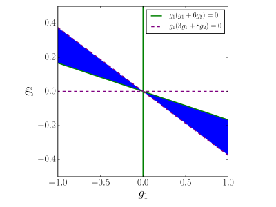
Figure 1: Parameter region consistent with the condition Eq. (15). Blue region is allowed.

4.2 Potential of $\varphi_{S}$

Next, let us turn to the $\varphi_{S}$ sector. It is convenient to work with the transformed basis:

$$\begin{pmatrix}\widetilde{\varphi}_{S1}\\ \widetilde{\varphi}_{S2}\\ \widetilde{\varphi}_{S3}\end{pmatrix}=U\begin{pmatrix}\varphi_{S1}\\ \varphi_{S2}\\ \varphi_{S3}\end{pmatrix},~{}~{}~{}~{}~{}U\equiv\begin{pmatrix}1/\sqrt{3}&1/\sqrt{3}&1/\sqrt{3}\\ 0&-1/\sqrt{2}&1/\sqrt{2}\\ -\sqrt{2}/\sqrt{3}&1/\sqrt{6}&1/\sqrt{6}\end{pmatrix}.$$ (16)

In this basis, the aligned vacuum in Eq. (3) becomes

$$\left<\widetilde{\varphi}_{S}\right>=(\widetilde{v}_{S},0,0).$$ (17)

We get a vacuum at

$$\widetilde{v}_{S}=\left(\frac{1}{5}\right)^{1/8}\left(\frac{m_{S}\Lambda^{3}}{g_{3}+g_{4}}\right)^{1/4}.$$ (18)

Again we ignore the $V_{A}$ term, which is justified as far as $m_{3/2}\ll m_{S}$. Expanding the flavon fields around the vacuum as

$$\widetilde{\varphi}_{S1}=\widetilde{v}_{S}+\frac{1}{\sqrt{2}}(\widetilde{\varphi}_{S1}^{R}+i\widetilde{\varphi}_{S1}^{I}),~{}~{}~{}\widetilde{\varphi}_{S2}=\frac{1}{\sqrt{2}}(\widetilde{\varphi}_{S2}^{R}+i\widetilde{\varphi}_{S2}^{I}),~{}~{}~{}\widetilde{\varphi}_{S3}=\frac{1}{\sqrt{2}}(\widetilde{\varphi}_{S3}^{R}+i\widetilde{\varphi}_{S3}^{I}),$$ (19)

we find out that $\widetilde{\varphi}_{S1}^{R}$ obtains a mass-squared of $8m_{S}^{2}$. On the other hand, $\varphi_{S2}^{R}$ and $\varphi_{S3}^{R}$ are mixed with each other. Their mass matrix is

$$\mathcal{M}_{R}^{2}=-\frac{m_{S}^{2}}{5(g_{3}+g_{4})^{2}}\begin{pmatrix}8g_{3}^{2}+13g_{3}g_{4}+2g_{4}^{2}&2\sqrt{3}(g_{3}+g_{4})g_{4}\\ 2\sqrt{3}(g_{3}+g_{4})g_{4}&3g_{4}(3g_{3}+2g_{4})\end{pmatrix}.$$ (20)

The condition that both of them have positive mass eigenvalues is

$$g_{3}g_{4}<0~{}~{}~{}{\rm and}~{}~{}~{}8g_{3}^{2}+17g_{3}g_{4}+8g_{4}^{2}<0.$$ (21)

Parameter regions consistent with this condition are shown in Fig. 2. The same condition also ensures that $\varphi_{S2}^{I}$ and $\varphi_{S3}^{I}$ have positive mass-squared eigenvalues. All of them have masses of $\mathcal{O}(m_{S}^{2})$. The only exception is $\varphi_{S1}^{I}$, which obtains a mass only from the $V_{A}$ term. Its mass-squared is $\mathcal{O}(m_{S}m_{3/2})$, lighter than the other scalar components, and has a positive sign if $g_{3}+g_{4}>0$ $(g_{3}+g_{4}<0)$ if $A>0$ $(A<0)$. Thus, the $\varphi_{S}$ field is successfully stabilized at the vacuum of Eq. (3).

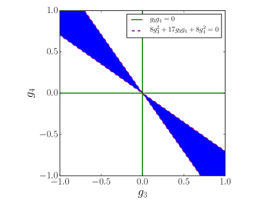
Figure 2: Parameter region consistent with the condition Eq. (21). Blue region is allowed.

4.3 Fermionic components

So far we obtained the desired aligned vacuum of Eq. (3). We now discuss the mass matrix of the fermionic components of the flavons $\varphi_{T}$ and $\widetilde{\varphi}_{S}$, which we call flavinos denoted by $\psi_{T}$ and $\widetilde{\psi}_{S}$, respectively. Flavinos become massive after flavons obtain VEVs. For the $\varphi_{T}$ sector, the flavino mass matrix is given by

$$\mathcal{M}_{\psi_{T}}=-\frac{m_{T}}{\sqrt{5}(g_{1}+4g_{2})}\begin{pmatrix}5(g_{1}+4g_{2})&0&0\\ 0&0&g_{1}-4g_{2}\\ 0&g_{1}-4g_{2}&0\end{pmatrix}.$$ (22)

For the $\widetilde{\varphi}_{S}$ sector, on the other hand, we have

$$\mathcal{M}_{\widetilde{\psi}_{S}}=-\frac{m_{S}}{\sqrt{5}(g_{3}+g_{4})}\begin{pmatrix}5(g_{3}+g_{4})&0&0\\ 0&-g_{3}+g_{4}/2&-\sqrt{3}g_{4}/2\\ 0&-\sqrt{3}g_{4}/2&g_{3}-g_{4}/2\end{pmatrix}.$$ (23)

Thus, all of them have masses of the order of the soft SUSY breaking mass scale.

4.4 Effects of other terms

We neglect many terms that are allowed by our charge assignments in the flavon superpotential Eq. (8). Thanks to the $Z_{12}$ and U(1)_R charges, the $\varphi_{T}$ sector, which gives the diagonal mass matrix of the charged leptons, is completely decoupled from the $\varphi_{S}$ and $\xi$ sector, which makes the tri-bimaximal form of the neutrino mixing matrix. There are eleven possible contractions of $\varphi_{T}^{6}$ that transform as 1 as a whole, while there are seventeen possible contractions for the $\varphi_{S}$ and $\xi$ sector.

The effect of these terms can be estimated using some symmetry argument as follows. First, we focus on the $\varphi_{T}$ sector. If we refer to one of the diagonalized elements of $A_{4}$, e.g. $T$ described in Appendix A, we can see that each component of the flavon transforms as $\{\varphi_{T1},\varphi_{T2},\varphi_{T3}\}\to\{\varphi_{T1},\omega\varphi_{T2},\omega^{2}\varphi_{T3}\}$ under $T$, where $\omega\equiv e^{2\pi i/3}$. Thus, the $\varphi_{T}$ sector of the most general flavon superpotential in our model, which should be invariant under $A_{4}$, takes the form of

$$W_{\rm f}^{(T)}\sim\frac{1}{\Lambda^{3}}\left(\varphi_{T1}^{6}+\varphi_{T1}^{4}\varphi_{T2}\varphi_{T3}+\cdots\right),$$ (24)

where the dots denote terms with more than two powers of $\{\varphi_{T2},\varphi_{T3}\}$. Here, we omit all the $\mathcal{O}(1)$ coefficients for simplicity. It is straightforward from Eq. (24) to see that $\varphi_{T}=(v_{T},0,0)$ always expresses one of the extrema of the potential with a properly chosen value of $v_{T}$ thanks to the absence of terms linear in $\{\varphi_{T2},\varphi_{T3}\}$. Regarding the curvature of the potential around the extremum, it is non-trivial to see whether the point we are considering is a local minimum, a local maximum, or a saddle point. However, we have already shown in Sec. 4.1 that the potential has a minimum at $\varphi_{T}=(v_{T},0,0)$ for some parameter spaces spanned by $g_{1}$ and $g_{2}$. Therefore, our flavon stabilization mechanism works well at least in the vicinity of such a parameter region.

Next, we consider the $\varphi_{S}$ and $\xi$ sector. Again, it is convenient to move to the basis expressed in Eq. (16). In this basis, one of the generators of $A_{4}$, which is denoted as $S$ in Appendix A, becomes diagonal:

$$\widetilde{S}\equiv USU^{-1}=\left(\begin{array}[]{ccc}1&0&0\\ 0&-1&0\\ 0&0&-1\\ \end{array}\right).$$ (28)

Therefore, the $\varphi_{S}$ and $\xi$ sector of the most general flavon superpotential has the form of

$$W_{\rm f}^{(S)}\sim\frac{1}{\Lambda^{3}}\left(\widetilde{\varphi}_{S1}^{6}+\widetilde{\varphi}_{S1}^{5}\xi+\widetilde{\varphi}_{S1}^{4}(\widetilde{\varphi}_{S2}^{2}+\widetilde{\varphi}_{S2}\widetilde{\varphi}_{S3}+\widetilde{\varphi}_{S3}^{2}+\xi^{2})+\cdots\right),$$ (29)

where the dots represent terms with more than two powers of $\{\widetilde{\varphi}_{S2},\widetilde{\varphi}_{S3},\xi\}$. Again, we omit all $\mathcal{O}(1)$ coefficients. It can be seen that the same argument as for the $\varphi_{T}$ sector follows, i.e., $\widetilde{\varphi}_{S}=(\widetilde{v}_{S},0,0)$ always remains an extremum of the potential and hence our flavon stabilization mechanism works well in some parameter regions at least in the vicinity of those shown in Sec. 4.2.

We would also like to explain the deviation from the tri-bimaximal form of the observed neutrino mixing matrix. For this purpose, we follow the procedure described in Refs. [13, 14] and consider a new flavon $\xi^{\prime}$ that has charges $\{\textbf{1}^{\prime},\rho^{2},1/3\}$ under our set up. Again, we can find out an example parameter region that stabilizes the flavon potential: we should just add a term proportional to $\xi^{{}^{\prime}6}$ to the superpotential Eq. (4) and a term $-m_{\xi^{\prime}}^{2}|\xi^{{}^{\prime}}|^{2}$ to the SUSY breaking potential Eq. (9). In this simple example, $\xi^{\prime}$ is completely decoupled from other fields in the scalar potential and the minimization condition of the potential remains unchanged except for the further condition for the $\xi^{\prime}$ VEV. When we consider other possible contractions in the superpotential, the number of allowed terms consist of $\{\varphi_{S},\xi,\xi^{\prime}\}$ is increased to twenty-nine. However, the above discussion still holds and there exists a finite volume region of the parameter space that is consistent with our scenario.

5 Solution to the domain wall problem

Although the flavor structure can be well described by the discrete flavor symmetry with proper VEV alignment of flavon fields, the domain wall problem arises if the spontaneous breaking of the flavor symmetry occurs after inflation, because there are many degenerate minima of the flavon potential. In this section, we show that our mechanism of the flavon stabilization described in Sec. 4 results in a simple and natural description of the cosmological dynamics of the flavon fields that does not lead to the formation of domain walls.

The cosmological flavon dynamics depends on the soft mass $m_{\rm soft}$, which collectively denote the soft SUSY breaking masses of flavons, and the Hubble parameter $H$. If $m_{\rm soft}\gtrsim H$ during inflation, flavons fall into one of the potential minima dynamically and such a region expands that covers the whole observable Universe without domain walls.

If $m_{\rm soft}\lesssim H$ during inflation, on the other hand, we need to include the negative Hubble-induced mass term during and after inflation as [17, 18]

$$V_{\rm SB}=-c_{T}H^{2}\sum_{i=1}^{3}|\varphi_{Ti}|^{2}-c_{S}H^{2}\sum_{i=1}^{3}|\varphi_{Si}|^{2}-c_{\xi}H^{2}|\xi|^{2},$$ (30)

where $c_{T}$, $c_{S}$, and $c_{\xi}$ are positive constants of order unity. These terms may come from the Planck-suppressed coupling among the inflaton and flavon fields in the Kähler potential. Since these negative Hubble-induced mass terms have the same form as the negative soft mass terms Eq. (9), the structure of the minima is the same as those discussed in Sec. 4 with $m_{\rm soft}$ being replaced by $H$, which is typically much larger than $m_{\rm soft}$. Then, during the inflation, the flavons will settle down into the minimum of the potential at the VEVs,

$$\left<\varphi_{T}\right>=(v^{H}_{T},0,0),~{}~{}~{}\left<\varphi_{S}\right>=(v^{H}_{S},v^{H}_{S},v^{H}_{S}),~{}~{}~{}\left<\xi\right>=v^{H}_{\xi},$$ (31)

where

$$v^{H}_{T},v^{H}_{S},v^{H}_{\xi}\sim\left(\frac{H\Lambda^{n-3}}{n-1}\right)^{1/(n-2)},$$ (32)

since the flavons have masses of $\mathcal{O}(H)$ around this temporal minimum. Domain walls are thus inflated away no matter what happens before inflation.

After inflation, as the Hubble parameter decreases, the VEV of the temporal minimum Eq. (31) becomes smaller, and we expect that the flavons will track the temporal minimum. In order for this to happen, there is a lower bound on $n$ in Eq. (4) depending on the background equation of state of the Universe as [20]

$$n\geq\frac{6p}{3p-1}=\begin{cases}4&{\rm for}~{}p=2/3,\\ 6&{\rm for}~{}p=1/2,\end{cases}$$ (33)

where $p$ is defined as the power law exponent of the cosmic scale factor: $a(t)\propto t^{p}$, hence $p=2/3$ $(1/2)$ for the matter (radiation) dominated Universe. If this condition is satisfied, flavons smoothly relax to the true potential minimum as $H$ becomes smaller than $m_{\rm soft}$. Otherwise, the flavon oscillations around the temporal minimum may be relatively enhanced as the Universe expands and flavons may overshoot the origin of the potential [20], which makes the whole flavon dynamics much more complicated and the domain wall formation may occur.

Since our model Eq. (8) corresponds to the $n=6$ case, the flavon fields do track the temporal minima of Eq. (31), and no symmetry restoration occurs after inflation if the inflaton effectively behaves as matter or radiation before the completion of reheating after inflation. Therefore, there are no domain walls in the observable Universe. This is a simple way to solve the domain wall problem in models with discrete flavor symmetry.

6 Conclusions and discussion

We have proposed a simple mechanism to stabilize the flavon potential in the model with discrete flavor symmetry. It is achieved by the balance between the negative soft mass and non-renormalizable terms with appropriate charge assignments of the flavon fields. The flavon sector is significantly simplified and the domain wall problem is naturally solved. Although we have focused on the $A_{4}$ model as a concrete setup, a similar mechanism should also work in models with other discrete symmetries in general. We leave this issue as future work.

Finally, we briefly discuss the cosmological aspects of this model. Most flavons have masses of $m_{\rm soft}$ around the vacuum and some flavons may be as light as $\sqrt{m_{3/2}m_{\rm soft}}$ if $m_{3/2}\lesssim m_{\rm soft}$ as shown in Sec. 4. Flavons in the $\varphi_{T}$ sector eventually decay into a Higgs boson plus 2 leptons (and possibly their superpartners depending on the mass spectrum), and its lifetime is typically much shorter than 1 sec, which does not affect the Big-Bang nucleosynthesis. Flavons in the $\varphi_{S}$ and $\xi$ sector decay into 2 Higgs bosons plus 2 leptons (and possibly their superpartners). Since their decay rate is suppressed by $\Lambda^{4}$, the lifetime can be much longer than 1 sec for $m_{S}\ll 1000\,$TeV and $\Lambda\sim 10^{12}\,$GeV and may affect Big-Bang nucleosynthesis. In such a case, we may need relatively low reheating temperature to avoid the overproduction of flavons, which are dominantly in the form of coherent oscillation. Flavinos, the fermionic superpartners of the flavons, also have masses of $\sim m_{\rm soft}$. For $m_{3/2}\lesssim m_{\rm soft}$, flavinos may decay into the gravitino and it can be a dominant source of the gravitino production depending on the reheating temperature. The gravitino decays into lighter SUSY particles unless the gravitino is the lightest, and the final dark matter abundance is determined either by the gravitino decay or thermal production, as usual.

Appendix A Notes on $A_{4}$ representations

It is known that all the elements of the $A_{4}$ group can be written as products of two elements $S$ and $T$, which are the generators of the subgroup $Z_{2}$ and $Z_{3}$, respectively. $A_{4}$ has a triplet representation 3 and three singlet representations 1, $\textbf{1}^{\prime}$, and $\textbf{1}^{\prime\prime}$. We adopt a basis of the triplet representation that diagonalizes $T$. In this basis, all the elements of $A_{4}$ are represented as

$$1=\begin{pmatrix}1&0&0\\ 0&1&0\\ 0&0&1\end{pmatrix},~{}~{}~{}T=\begin{pmatrix}1&0&0\\ 0&\omega&0\\ 0&0&\omega^{2}\end{pmatrix},~{}~{}~{}T^{2}=\begin{pmatrix}1&0&0\\ 0&\omega^{2}&0\\ 0&0&\omega\end{pmatrix},$$ (34)

$$S=\frac{1}{3}\begin{pmatrix}-1&2&2\\ 2&-1&2\\ 2&2&-1\end{pmatrix},~{}ST=\frac{1}{3}\begin{pmatrix}-1&2\omega&2\omega^{2}\\ 2&-\omega&2\omega^{2}\\ 2&2\omega&-\omega^{2}\end{pmatrix},~{}ST^{2}=\frac{1}{3}\begin{pmatrix}-1&2\omega^{2}&2\omega\\ 2&-\omega^{2}&2\omega\\ 2&2\omega^{2}&-\omega\end{pmatrix},$$ (35)

$$TS=\frac{1}{3}\begin{pmatrix}-1&2&2\\ 2\omega&-\omega&2\omega\\ 2\omega^{2}&2\omega^{2}&-\omega^{2}\end{pmatrix},~{}TST=\frac{1}{3}\begin{pmatrix}-1&2\omega&2\omega^{2}\\ 2\omega&-\omega^{2}&2\\ 2\omega^{2}&2&-\omega\end{pmatrix},~{}TST^{2}=\frac{1}{3}\begin{pmatrix}-1&2\omega^{2}&2\omega\\ 2\omega&-1&2\omega^{2}\\ 2\omega^{2}&2\omega&-1\end{pmatrix},$$ (36)

$$T^{2}S=\frac{1}{3}\begin{pmatrix}-1&2&2\\ 2\omega^{2}&-\omega^{2}&2\omega^{2}\\ 2\omega&2\omega&-\omega\end{pmatrix},~{}T^{2}ST=\frac{1}{3}\begin{pmatrix}-1&2\omega&2\omega^{2}\\ 2\omega^{2}&-1&2\omega\\ 2\omega&2\omega^{2}&-1\end{pmatrix},~{}T^{2}ST^{2}=\frac{1}{3}\begin{pmatrix}-1&2\omega^{2}&2\omega\\ 2\omega^{2}&-\omega&2\\ 2\omega&2&-\omega^{2}\end{pmatrix},$$ (37)

where we define $\omega\equiv e^{2\pi i/3}$. The product of two triplets are decomposed as $\textbf{3}\times\textbf{3}=\textbf{1}+\textbf{1}^{\prime}+\textbf{1}^{\prime\prime}+\textbf{3}_{S}+\textbf{3}_{A}$. For each contraction, we use the convention of the coefficient as follows:

$${\bf 1}\sim a_{1}b_{1}+a_{2}b_{3}+a_{3}b_{2}\equiv(ab),$$ (38)

$${\bf 1}^{\prime}\sim a_{3}b_{3}+a_{1}b_{2}+a_{2}b_{1}\equiv(ab)^{\prime},$$ (39)

$${\bf 1}^{\prime\prime}\sim a_{2}b_{2}+a_{3}b_{1}+a_{1}b_{3}\equiv(ab)^{\prime\prime},$$ (40)

$${\bf 3}_{S}\sim\begin{pmatrix}2a_{1}b_{1}-a_{2}b_{3}-a_{3}b_{2}\\ 2a_{3}b_{3}-a_{1}b_{2}-a_{2}b_{1}\\ 2a_{2}b_{2}-a_{3}b_{1}-a_{1}b_{3}\end{pmatrix}\equiv(ab)_{\bf 3_{S}},~{}~{}~{}{\bf 3}_{A}\sim\begin{pmatrix}a_{2}b_{3}-a_{3}b_{2}\\ a_{1}b_{2}-a_{2}b_{1}\\ a_{3}b_{1}-a_{1}b_{3}\end{pmatrix}\equiv(ab)_{\bf 3_{A}},$$ (41)

where $a=(a_{1},a_{2},a_{3})$ and $b=(b_{1},b_{2},b_{3})$ are triplets.

For the product of the same triplet $\varphi=(\varphi_{1},\varphi_{2},\varphi_{3})$, we have

$$(\varphi^{2})=\varphi_{1}^{2}+2\varphi_{2}\varphi_{3},~{}~{}~{}(\varphi^{2})^{\prime}=\varphi_{3}^{2}+2\varphi_{1}\varphi_{2},~{}~{}~{}(\varphi^{2})^{\prime\prime}=\varphi_{2}^{2}+2\varphi_{3}\varphi_{1},$$ (42)

$$(\varphi^{2})_{\bf 3_{S}}=2\begin{pmatrix}\varphi_{1}^{2}-\varphi_{2}\varphi_{3}\\ \varphi_{3}^{2}-\varphi_{1}\varphi_{2}\\ \varphi_{2}^{2}-\varphi_{3}\varphi_{1}\end{pmatrix},~{}~{}~{}(\varphi^{2})_{\bf 3_{A}}=0,$$ (43)

$$(\varphi^{3})_{\bf 1}=2(\varphi_{1}^{3}+\varphi_{2}^{3}+\varphi_{3}^{3}-3\varphi_{1}\varphi_{2}\varphi_{3}).$$ (44)

In terms of the transformed basis $\widetilde{\varphi}$ in Eq. (16), they become

$$(\widetilde{\varphi}^{2})=\widetilde{\varphi}_{1}^{2}-\widetilde{\varphi}_{2}^{2}+\widetilde{\varphi}_{3}^{2},$$ (45)

$$(\widetilde{\varphi}^{2})^{\prime}=\widetilde{\varphi}_{1}^{2}+\frac{1}{2}(\widetilde{\varphi}_{2}^{2}+2\sqrt{3}\widetilde{\varphi}_{2}\widetilde{\varphi}_{3}-\widetilde{\varphi}_{3}^{2}),$$ (46)

$$(\widetilde{\varphi}^{2})^{\prime\prime}=\widetilde{\varphi}_{1}^{2}+\frac{1}{2}(\widetilde{\varphi}_{2}^{2}-2\sqrt{3}\widetilde{\varphi}_{2}\widetilde{\varphi}_{3}-\widetilde{\varphi}_{3}^{2}),$$ (47)

$$(\widetilde{\varphi}^{2})_{\bf 3_{S}}=\begin{pmatrix}\widetilde{\varphi}_{2}^{2}+\widetilde{\varphi}_{3}^{2}-2\sqrt{2}\widetilde{\varphi}_{1}\widetilde{\varphi}_{3}\\ \widetilde{\varphi}_{2}^{2}+\widetilde{\varphi}_{3}^{2}+\sqrt{2}\widetilde{\varphi}_{1}(\sqrt{3}\widetilde{\varphi}_{2}+\widetilde{\varphi}_{3})\\ \widetilde{\varphi}_{2}^{2}+\widetilde{\varphi}_{3}^{2}+\sqrt{2}\widetilde{\varphi}_{1}(-\sqrt{3}\widetilde{\varphi}_{2}+\widetilde{\varphi}_{3})\end{pmatrix},~{}~{}~{}(\widetilde{\varphi}^{2})_{\bf 3_{A}}=0,$$ (48)

$$(\widetilde{\varphi}^{\,3})_{\bf 1}=3\sqrt{3}\widetilde{\varphi}_{1}(\widetilde{\varphi}_{2}^{2}+\widetilde{\varphi}_{3}^{2}).$$ (49)

References

• [1] G. Altarelli and F. Feruglio, Rev. Mod. Phys.  82, 2701 (2010) [arXiv:1002.0211 [hep-ph]].
• [2] H. Ishimori, T. Kobayashi, H. Ohki, Y. Shimizu, H. Okada and M. Tanimoto, Prog. Theor. Phys. Suppl.  183, 1 (2010) [arXiv:1003.3552 [hep-th]].
• [3] S. F. King, A. Merle, S. Morisi, Y. Shimizu and M. Tanimoto, New J. Phys.  16, 045018 (2014) [arXiv:1402.4271 [hep-ph]].
• [4] S. F. King, Prog. Part. Nucl. Phys.  94, 217 (2017) [arXiv:1701.04413 [hep-ph]].
• [5] A. Vilenkin and E. P. S. Shellard, “Cosmic Strings and Other Topological Defects,” Cambridge University Press.
• [6] F. Riva, Phys. Lett. B 690, 443 (2010) [arXiv:1004.1177 [hep-ph]].
• [7] S. Antusch and D. Nolde, JCAP 1310, 028 (2013) [arXiv:1306.3501 [hep-ph]].
• [8] S. Chigusa and K. Nakayama, arXiv:1808.09601 [hep-ph].
• [9] S. F. King and Y. L. Zhou, arXiv:1809.10292 [hep-ph].
• [10] G. Altarelli and F. Feruglio, Nucl. Phys. B 741, 215 (2006) [hep-ph/0512103].
• [11] P. F. Harrison, D. H. Perkins and W. G. Scott, Phys. Lett. B 530 (2002) 167 [hep-ph/0202074].
• [12] E. Ma and G. Rajasekaran, Phys. Rev. D 64, 113012 (2001) [hep-ph/0106291].
• [13] Y. Shimizu, M. Tanimoto and A. Watanabe, Prog. Theor. Phys.  126, 81 (2011) [arXiv:1105.2929 [hep-ph]].
• [14] S. K. Kang, Y. Shimizu, K. Takagi, S. Takahashi and M. Tanimoto, PTEP 2018, no. 8, 083B01 (2018) [arXiv:1804.10468 [hep-ph]].
• [15] I. de Medeiros Varzielas, T. Neder and Y. L. Zhou, Phys. Rev. D 97 (2018) no.11, 115033 [arXiv:1711.05716 [hep-ph]].
• [16] D. H. Lyth and E. D. Stewart, Phys. Rev. D 53, 1784 (1996) [hep-ph/9510204].
• [17] M. Dine, L. Randall and S. D. Thomas, Phys. Rev. Lett.  75, 398 (1995) [hep-ph/9503303].
• [18] M. Dine, L. Randall and S. D. Thomas, Nucl. Phys. B 458, 291 (1996) [hep-ph/9507453].
• [19] S. Kasuya, M. Kawasaki and F. Takahashi, JCAP 0810, 017 (2008) [arXiv:0805.4245 [hep-ph]].
• [20] Y. Ema, K. Nakayama and M. Takimoto, JCAP 1602, no. 02, 067 (2016) [arXiv:1508.06547 [gr-qc]].