Atmospheric dynamics and the variable transit of KELT-9 b

Abstract

We present a spectrally and temporally resolved detection of the optical Mg I triplet at 7.8$\sigma$ in the extended atmosphere of the ultra-hot Jupiter KELT-9 b, adding to the list of detected metal species in the hottest gas giant currently known. Constraints are placed on the density and radial extent of the excited hydrogen envelope using simultaneous observations of H$\alpha$ and H$\beta$ under the assumption of a spherically symmetric atmosphere. We find that planetary rotational broadening of $v_{\text{rot}}=8.2^{+0.6}_{-0.7}$ km s^-1 is necessary to reproduce the Balmer line transmission profile shapes, where the model including rotation is strongly preferred over the non-rotating model using a Bayesian information criterion comparison. The time-series of both metal line and hydrogen absorption show remarkable structure, suggesting that the atmosphere observed during this transit is dynamic rather than static. We detect a relative emission feature near the end of the transit which exhibits a P-Cygni-like shape, evidence of material moving at $\approx 50-100$ km s^-1 away from the planet. We hypothesize that the in-transit variability and subsequent P-Cygni-like profiles are due to a flaring event that caused the atmosphere to expand, resulting in unbound material being accelerated to high speeds by stellar radiation pressure. Further spectroscopic transit observations will help establish the frequency of such events.

1 INTRODUCTION

Massive gas giants in short orbital periods ($P_{\text{orb}}\lesssim 10$ days) are laboratories for probing unusual planetary atmospheric conditions and star-planet interactions. The high UV insolation levels experienced by these planets can cause extreme atmospheric mass loss (Vidal-Madjar et al. 2003; Murray-Clay et al. 2009; Lecavelier des Etangs et al. 2012; Owen & Jackson 2012; Kulow et al. 2014; Ehrenreich et al. 2015) and high-velocity winds and zonal jets (Showman et al. 2008; Rauscher & Menou 2010; Rauscher & Kempton 2014; Louden & Wheatley 2015; Brogi et al. 2016), while orbits near the Alfvén radius can lead to observable magnetic interactions between the planet and star (Cuntz et al. 2000; Shkolnik et al. 2005, 2008; Lanza 2009; Strugarek et al. 2014; Cauley et al. 2018a) and pre-transit signatures due to shocked stellar or planetary wind material (Fossati et al. 2010; Vidotto et al. 2010; Llama et al. 2011, 2013; Cauley et al. 2015, 2018b).

The atmospheres of transiting hot planets are readily probed via transmission spectroscopy, which can reveal the presence of individual atomic (e.g., Redfield et al. 2008; Snellen et al. 2008; Jensen et al. 2011, 2012; Pont et al. 2013; Cauley et al. 2015; Wilson et al. 2015; Wyttenbach et al. 2015, 2017; Casasayas-Barris et al. 2017, 2018; Spake et al. 2018; Jensen et al. 2018) and molecular species (e.g., Knutson et al. 2007; Snellen et al. 2010; Deming et al. 2013; Kreidberg et al. 2015; Brogi et al. 2016; Sing et al. 2016), measure the dynamics of planetary rotation and winds (Bourrier et al. 2015; Louden & Wheatley 2015; Brogi et al. 2016), and detect hazes and cloud layers (Knutson et al. 2014; Mallonn & Strassmeier 2016; Kreidberg et al. 2018; Chen et al. 2018). Optical transmission spectra generally target strong atomic lines, such as Na I D, K I 7698 Å, and H$\alpha$, which probe the thermosphere at pressures of $\approx 1\mu$bar (Heng et al. 2015; Huang et al. 2017). Recently, He I 10830 Å was detected in the extended atmospheres of WASP-107 b and HAT-P-11 b, demonstrating the line’s potential as a mass loss diagnostic for hot planets (Spake et al. 2018; Mansfield et al. 2018; Oklopc̆ić & Hirata 2018).

The hottest gas giant discovered so far is KELT-9 b (Gaudi et al. 2017), which orbits at a distance of $0.034$ AU from its A0V/B9V host star ($T_{\text{eff}}=10170\pm 450$ K) with a dayside equilibrium temperature of $T_{\text{eq}}\approx 4600$ K. Kitzmann et al. (2018) showed that KELT-9 b’s high temperature, which should dissociate most refractory molecules into their constituent atoms, could produce a suite of observable Fe I and Fe II lines in the optical. This prediction was validated by Hoeijmakers et al. (2018) who detected a strong cross-correlation signal in optical Fe I, Fe II, and Ti II lines. Yan & Henning (2018), via absorption at H$\alpha$, detected the presence of an optically thick layer of excited hydrogen around KELT-9 b and estimated the planetary mass loss rate to be $\sim 10^{12}$ g s^-1.

The metal detections from Hoeijmakers et al. (2018) were made by cross-correlating a large number of theoretical iron line absorption cross sections with in-transit spectra obtained with HARPS-N on the 3.58-meter Telescopio Nazionale Galileo (TNG). The H$\alpha$ observations of Yan & Henning (2018) were also acquired with a 3.5-meter telescope (the 3.5-meter at Calar Alto Observatory). While the cross correlation technique is powerful when a large number of lines are present in the spectrum, the detection of weak transmission spectrum absorption of individual spectral lines during a single transit, as opposed to the strong ($\approx 1\%$) signal seen in H$\alpha$ (Yan & Henning 2018), requires the use of 10-meter class telescopes combined with efficient high-resolution spectrographs.

Here we present the first exoplanet atmosphere detection of the optical Mg I triplet around KELT-9 b using the PEPSI spectrograph (Strassmeier et al. 2015) on the Large Binocular Telescope (LBT; $2\times 8.4$ m). Magnesium absorption can be used to estimate exoplanet mass loss rates (Bourrier et al. 2015) and is an important coolant in hot planet atmospheres (Huang et al. 2017). We also confirm the H$\alpha$ measurement of Yan & Henning (2018) and provide additional constraints on the extended hydrogen atmosphere using simultaneous observations of H$\beta$. Atmospheric models of the Mg I and Balmer line absorption favor non-zero planetary rotation velocities. Finally, we observe significant in-transit variability in all of the planetary absorption lines and large blue-shifted velocities in the transmission profiles near the end of the transit. We hypothesize that a stellar flare event is responsible for the variability and an increase in the planet’s mass loss rate, where the expanding material is accelerated to high velocities by stellar radiation pressure.

2 OBSERVATIONS AND DATA REDUCTION

We observed the transit of KELT-9 b between 04:07–11:20 UT on July 3, 2018 with the Large Binocular Telescope in Arizona and its high-resolution échelle spectrograph PEPSI (Strassmeier et al. 2015). PEPSI is a white-pupil échelle spectrograph with two arms (blue and red optimized) and is equipped with six cross dispersers (CD I to VI) for full optical wavelength coverage. Sky fibers for simultaneous sky and target exposures are available but were not used for the present observations. In use for the data in this paper was the new image slicer block #3. Its $R\approx 50,000$-mode employs two three-slice waveguide image slicers and a pair of 300-$\mu$m fibers with a projected sky aperture of 2.3^′′. Seeing for the night was $\approx 1^{\prime\prime}$. Two 10.3k$\times$10.3k STA1600LN CCDs with 9-$\mu$m pixels recorded a total of 34 échelle orders in CD III and V together. One spectral resolution element corresponds to 0.10 Å in the blue and 0.14 Å in the red ($\approx$6 km s^-1) and is sampled with 12.4 pixels. The dispersion changes from 8 mÅ pixel^-1 at 4000 Å to 18 mÅ pixel^-1 at 9000 Å and results in an unequally spaced pixel-step size.

PEPSI was used in its $R\approx 50,000$ mode and with cross dispersers (CD) III (blue arm) and V (red arm) simultaneously. The wavelength coverage was 4750–5430 Å in the blue arm and 6230–7430 Å in the red arm. The spectra were collected with a constant signal-to-noise of 210 in the continuum controlled by a photon counter. This results in slightly different exposure times for each CD and produced 82 blue arm spectra and 73 red arm spectra, with exposure times between 220 s and 300 s depending on air mass.

All data were reduced with the Spectroscopic Data System for PEPSI (SDS4PEPSI) which is a generic software package written in C++ under a Linux environment. The standard reduction steps include bias overscan detection and subtraction, scattered light surface extraction from the inter-order space and subsequent subtraction, definition of échelle orders, optimal extraction of spectral orders, wavelength calibration, and a self-consistent continuum fit to the full 2D image of extracted orders. Wavelength calibration was based on a standard Thorium-Argon (Th-Ar) hollow-cathode lamp. The spectrograph is located in a pressure-controlled chamber at a constant temperature and humidity to keep the refractive index of the air inside constant over a long-term period, which provides radial velocity stability of about 5 m s^-1. The ThAr spectra were taken just before observations started and no significant instabilities in radial velocity of the spectra were detected as a function of time. We employ a “super master” flat fielding procedure to correct for the spatial pixel-to-pixel noise on the CCD. The super-master flat is a polynomial fit to the amplitude of the spatial noise versus flux in each pixel of the master flat, which is an average of 5,000 flat exposures. This procedure is specific to the STA1600LN CCD. The individual science images are first flat fielded and then optimally extracted. More details on PEPSI data reduction can be found in Strassmeier et al. (2018). The extracted spectra are corrected for the Earth’s barycentric motion at the time of the observation.

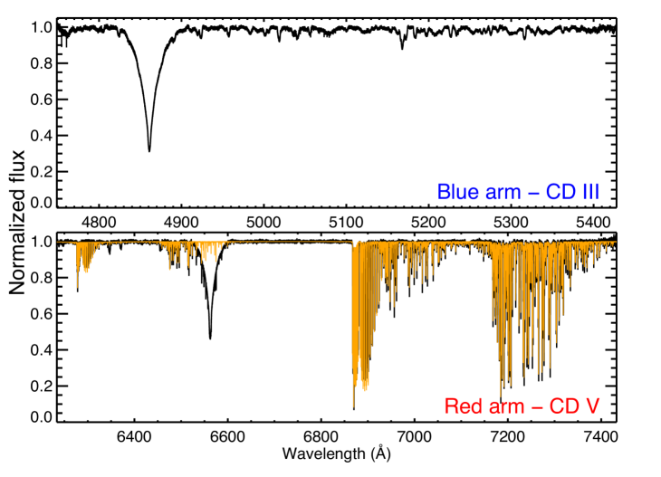
Figure 1: Individual KELT-9 spectrum (black) showing the full wavelength range of a PEPSI exposure using CDs III and V. The orange spectrum is the nominal telluric model, found with MOLECFIT, for the red arm. Note that the telluric spectrum has not been scaled to precisely match the telluric absorption lines.

2.1 Telluric line removal

Telluric line contamination is present throughout the red arm spectrum (see Figure 1). In order to remove the telluric lines, we used the software package MOLECFIT (Kausch et al. 2015; Smette et al. 2015). We fit regions of the average KELT-9 red arm spectrum that did not contain photospheric absorption. This mainly avoided the spectrum surrounding H$\alpha$ at 6562.79 Å. The nominal telluric model produced by MOLECFIT is shown in orange in Figure 1. We then fit the telluric absorption for individual exposures by scaling and shifting the nominal telluric model. We optimized the removal to focus on the telluric lines near H$\alpha$. We note that by doing this the strong telluric lines in other regions, e.g., the O₂ and H₂O band near 7200 Å, are not as cleanly removed. This is the result of line blending and imperfect model profile shapes, which exacerbates the residuals for strong lines. However, the poor correction in the strong lines does not affect the detection of transmission signatures in regions of weak or non-existant telluric absorption. The unblended weak telluric lines near H$\alpha$ are removed down to the photon noise level for individual spectra.

2.2 Center-to-limb variations

Center-to-limb variations, or CLVs, in spectral lines are the result of wavelength-dependent limb darkening across the stellar disk. CLVs can produce spurious transmission spectrum signals if not properly taken into account (e.g., Yan et al. 2015; Czesla et al. 2015; Khalafinejad et al. 2017; Yan et al. 2017; Cauley et al. 2017a). In order to remove the CLVs from our transmission spectra, we use the Spectroscopy Made Easy (SME) package (Valenti & Piskunov 1996; Piskunov & Valenti 2017) to generate synthetic spectra as a function of $\mu=\cos\theta$. We adopt the KELT-9 stellar parameters from Gaudi et al. (2017) for the model spectra (Table 1). The spectra are generated at 25 different $\mu$-values and interpolated onto the final stellar $\mu$-grid used in the transit simulations.

Table 1: KELT-9 system parameters

Parameter	Symbol	Units	Value
Stellar mass	$M_{\star}$	$M_{\sun}$	$2.52^{+0.25}_{-0.20}$
Stellar radius	$R_{\star}$	$R_{\sun}$	$2.362^{+0.075}_{-0.063}$
Effective temperature	$T_{\text{eff}}$	K	$10170\pm 450$
Metallicity	[Fe/H]	$\cdots$	$-0.03\pm 0.20$
Stellar rotational velocity	$v$sin$i$	km s-1	$111.4\pm 1.3$
Spin-orbit alignment angle	$\lambda$	degrees	$-84.8\pm 1.4$
Orbital period	$P_{\text{orb}}$	days	$1.4811235\pm 0.0000011$
Semi-major axis	$a$	AU	$0.03462^{+0.00110}_{-0.00093}$
Planetary mass	$M_{\text{p}}$	$M_{\text{J}}$	$2.88\pm 0.84$
Planetary radius	$R_{\text{p}}$	$R_{\text{J}}$	$1.891^{+0.061}_{-0.053}$
Orbital velocity†	$v_{\text{orb}}$	km s-1	$254.3\pm 8.1$

The in-transit CLV contributions are calculated by simulating the transit of KELT-9 b at the same times as our observations, taking into account the misaligned orbit of the planet and rotational broadening due to the $v$sin$i$ of the star. By taking into account stellar rotation and spin-orbit angle, we are also correcting for velocity shifts in the observed spectrum due to the Rossiter-McLaughlin (RM) effect. The planetary and orbital parameters are taken from Gaudi et al. (2017) (Table 1). We generate a spatial grid with resolution $0.01R_{\star}\times 0.01R_{\star}$ with the appropriate CLV- and RM-modified stellar spectrum assigned to each grid cell. We then integrate the in-transit stellar spectrum at the wavelengths of interest. The in-transit spectrum is then divided by the integrated out-of-transit spectrum. The result is the in-transit profile surrounding the desired spectral line. The in-transit profile can then be divided out of the observed transmission spectrum, leaving behind any atmospheric contribution from the planet (e.g., Khalafinejad et al. 2017; Yan & Henning 2018).

3 RESULTS

We identified absorption in the planetary atmosphere by creating an average transmission spectrum, which we denote as $S_{\text{T}}=S_{\text{in}}/S_{\text{out}}$, for each arm and automatically searching for significant deviations in the spectrum. The out-of-transit spectra ($N=37$ for the blue arm and $N=29$ for the red arm) were averaged to create a master $S_{\text{out}}$ spectrum. The average $S_{\text{T}}$ spectrum is the mean of all $S_{\text{T}}$ obtained between the second and third transit contact points, where the planet does not intersect the stellar limb. We shifted the individual $S_{\text{T}}$ spectra into the rest frame of the planet, eliminating the orbital velocity signature. The RV of the star is also removed. We performed the line search using Gaussian fits across the entire observed wavelength range and flagging any features with depths $\geq 1.5\sigma$ below the local continuum and FWHM values of $\geq 0.25$ Å. We then manually checked the flagged wavelengths confirm the presence of an absorption line; spurious signatures, e.g., artifacts from joined orders with overlapping wavelength regions, were discarded.

Absorption values for lines with detections at $\geq 3\sigma$ are given in Table 2, along with line depths, central velocities, and FWHM values derived by fitting a Gaussian using a Markov Chain Monte Carlo (MCMC) procedure based on the algorithm by Goodman & Weare (2010) (see also Foreman-Mackey et al. 2012). The absorption, which is given in equivalent angstroms, is calculated by integrating the transmission spectrum within $\pm 50$ km s^-1 of the line’s central air wavelength for the Balmer lines and $\pm 30$ km s^-1 for the narrower metal lines. The uncertainty in the average equivalent width $W_{\lambda}$ values is calculated by measuring the standard deviation of $S_{T}$ outside of the the absorption integration region but within $\pm 200$ km s^-1 and assigning this value as the error for each point in $S_{T}$. Detected lines with overlapping $\pm 200$ km s^-1 segments are ignored when calculating the absorption in one of the lines. The individual errors are then summed in quadrature to produce the final uncertainty given in column 4 of Table 2. The average $S_{\text{T}}$ profiles for the lines in Table 2 are shown in Figure 2 ordered by atomic weight and sub-ordered by wavelength. The uncertainties on the Gaussian line parameters are the 68% values from the marginalized posterior distributions.

Table 2: Average in-transit absorption and line parameters

	$\lambda_{0}$	$W_{\lambda}$	$\sigma_{\text{W}}$	Depth	$v_{\text{cen}}$	FWHM
Species	(Å)	(mÅ)	(mÅ)	(%)	(km s-1)	(km s-1)
Ti II	4805.09	0.60	0.15	$0.102^{+0.019}_{-0.016}$	$-5.27^{+2.61}_{-2.67}$	$30.5^{+15.1}_{-5.0}$
Fe I	4824.17	0.58	0.16	$0.134^{+0.014}_{-0.015}$	$-3.20^{+1.78}_{-1.56}$	$27.0^{+4.6}_{-3.2}$
H$\beta$	4861.35	6.45	0.27	$0.783^{+0.009}_{-0.010}$	$-0.97^{+0.35}_{-0.33}$	$49.8^{+0.7}_{-0.7}$
Fe II	4923.92	1.86	0.14	$0.414^{+0.017}_{-0.016}$	$1.76^{+0.45}_{-0.54}$	$24.7^{+1.5}_{-1.2}$
Fe I∗	4957.60	0.89	0.13	$0.121^{+0.012}_{-0.013}$	$-8.62^{+3.94}_{-7.84}$	$56.7^{+33.8}_{-13.1}$
Fe II	5018.44	2.28	0.14	$0.460^{+0.017}_{-0.015}$	$1.85^{+0.45}_{-0.64}$	$26.9^{+1.4}_{-1.1}$
Mg I	5167.32	0.99	0.13	$0.157^{+0.013}_{-0.014}$	$4.52^{+1.94}_{-1.85}$	$38.9^{+7.7}_{-4.7}$
Fe II	5169.03	2.40	0.12	$0.475^{+0.015}_{-0.014}$	$1.68^{+0.40}_{-0.44}$	$26.9^{+1.2}_{-1.0}$
Mg I	5172.68	1.01	0.13	$0.172^{+0.016}_{-0.015}$	$-1.33^{+1.25}_{-1.18}$	$30.3^{+4.8}_{-3.2}$
Mg I	5183.60	0.99	0.12	$0.157^{+0.016}_{-0.017}$	$-0.98^{+1.30}_{-1.44}$	$31.8^{+6.9}_{-4.1}$
Ti II	5188.69	0.61	0.12	$0.117^{+0.019}_{-0.016}$	$-1.30^{+1.85}_{-1.77}$	$29.6^{+11.4}_{-4.5}$
Fe II	5197.57	0.98	0.13	$0.184^{+0.015}_{-0.014}$	$1.43^{+1.08}_{-1.13}$	$28.9^{+3.8}_{-2.7}$
Ti II	5226.54	0.88	0.13	$0.142^{+0.014}_{-0.014}$	$2.89^{+1.64}_{-1.63}$	$32.8^{+6.3}_{-4.0}$
Fe II	5234.62	1.09	0.13	$0.173^{+0.012}_{-0.014}$	$0.92^{+1.23}_{-1.21}$	$34.7^{+4.7}_{-3.5}$
Fe II	5275.99	1.08	0.15	$0.268^{+0.017}_{-0.015}$	$1.18^{+0.61}_{-0.66}$	$20.9^{+1.8}_{-1.3}$
Fe II	5316.61	1.72	0.14	$0.317^{+0.015}_{-0.014}$	$2.54^{+0.60}_{-0.72}$	$28.0^{+2.1}_{-1.7}$
Fe II	5362.86	0.69	0.14	$0.154^{+0.016}_{-0.015}$	$-1.02^{+1.08}_{-1.26}$	$23.7^{+3.6}_{-2.3}$
Fe II	6456.38	1.34	0.13	$0.181^{+0.023}_{-0.017}$	$3.00^{+1.17}_{-1.46}$	$24.7^{+5.0}_{-2.7}$
H$\alpha$	6562.79	13.67	0.208	$1.103^{+0.010}_{-0.009}$	$2.67^{+0.25}_{-0.28}$	$55.1^{+0.6}_{-0.6}$

3.1 Hydrogen absorption

We confirm the H$\alpha$ absorption detected by Yan & Henning (2018) and report significant absorption in H$\beta$. The H$\alpha$ and H$\beta$ line profiles are shown in the first row of Figure 2. The depth ($1.103^{+0.010}_{-0.009}$%) and line width (FWHM $=55.1^{+0.7}_{-0.6}$ km s^-1) of H$\alpha$ is very similar to the Yan & Henning (2018) measurements ($1.15\pm 0.05$% and 51.2${}^{+2.7}_{-2.5}$ km s^-1, respectively) suggesting that the excited hydrogen layer is non-variable from epoch to epoch. H$\beta$ has a line depth of $0.783^{+0.009}_{-0.010}$% and FWHM$=49.8^{+0.7}_{-0.7}$ km s^-1. The large H$\beta$ line depth verifies that the hydrogen layer detected by Yan & Henning (2018) is optically thick.

3.2 Metal line absorption

In addition to the Fe I, Fe II, and Ti II signatures detected by Hoeijmakers et al. (2018) we report the presence of absorption in the Mg I 5167.3, 5172.7, 5183.6 Å triplet. The average $S_{T}$ spectra for all metal lines with absorption detected at $\geq 3\sigma$ are shown in Figure 2. The relative absorption depths of Fe I, Fe II, and Ti II are similar to the relative S/N of the cross-correlation functions from Hoeijmakers et al. (2018). We also analyze a control region of the spectrum where we do not expect to see planetary absorption. This region is shown in Figure 3 and consists of Cr II and Fe II lines with ground state energy levels of $E_{1}\approx 4-13$ eV, too high to be significantly populated in the atmosphere of KELT-9 b. Note that the abundance of hydrogen is what allows the $n=2$ state, which has an excitation energy of 10.2 eV, to be populated via radiative excitation (Huang et al. 2017) whereas less abundant metal species simply do not have sufficient number densities to produce observable populations of highly excited states.

The Mg I triplet shows absorption in each of the three lines. However, there is considerable contamination from nearby Fe I, Fe II, and Ti II lines (red lines in Figure 2). The triplet member at 5172.7 Å is relatively free of contaminants near the line core. The absorption in this line alone is significant at the level of $7.8\sigma$. The likelihood of the absorption being due to Mg I is strengthened by the similar absorption in the other triplet members.

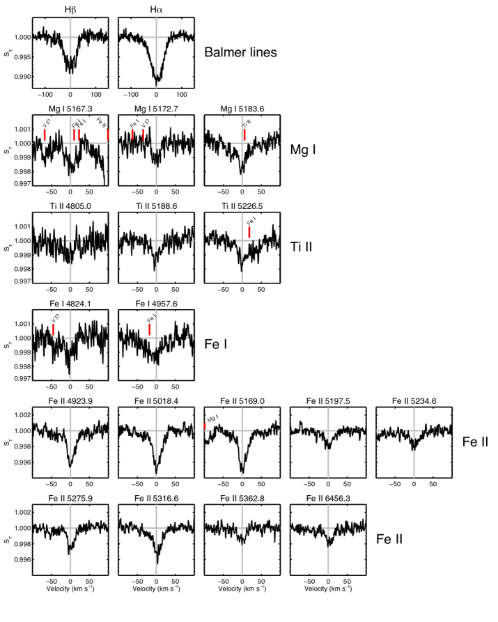
Figure 2: Average $S_{\text{T}}$ profiles for the lines with absorption detected at $\geq 3\sigma$ listed in order of atomic weight and from red to blue wavelengths within atomic species. Possible contaminating atomic transitions are marked with vertical red lines. All x-axis values are velocities in km s^-1. All lines of a particular atomic species are on the same vertical scale.

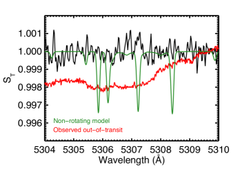
Figure 3: Average in-transit control region transmission spectrum. The green line shows the non-rotating stellar model and the presence of the strong lines Cr II 5305.85 Å, Fe II 5306.18 Å, Ca II 5307.22 Å, and Cr II 5308.41 Å in the stellar spectrum. The observed rotationally broadened KELT-9 out-of-transit spectrum is shown in red. There is no absorption present in the control region, demonstrating that the measured absorption in the metal lines is not an artifact.

3.3 Extended atmosphere models and planetary rotation

In order to place constraints on the density and structure of the extended atmosphere, we simulated the Balmer line and Mg I absorption using spherically symmetric atmospheres. We take the density in the atmosphere to be uniform. The uniform density case for hydrogen is consistent with the results of Christie et al. (2013) and Huang et al. (2017), who find that the $n=2$ hydrogen density is approximately constant across three orders of magnitude in pressure for the case of HD 189733 b’s atmosphere. For the Mg I triplet, we do not have strong constraints on the density due to the lack of additional Mg I transitions. As we will show, our Mg I measurement is consistent with an optically thin atmosphere and the density and radial extent of the atmosphere are not well constrained. Thus assuming a uniform density is a good first approximation.

The models consist of a 3-D grid, with spatial resolution $0.01R_{\star}\times 0.01R_{\star}\times 0.01R_{\star}$, filled with material of number density $n$ between $R_{\text{p}}$ and the radial extent of the atmosphere $r$. After the 3-D density grid is populated, the column density is calculated at each point intersecting the stellar disk. The 2-D column density grid is then used to extinct the stellar spectrum at the corresponding disk location. The extincted line profiles are then summed and the ratio is taken with the out-of-transit spectrum to create the model $S_{\text{T}}$ for the mean observed transit time. A Gaussian is assumed for the intrinsic line profile shape.

In addition to thermal broadening, which we take to be the intrinsic full-width at half maximum of the Gaussian $v_{\text{t}}$, we also consider the effects of atmospheric rotational broadening. KELT-9 b’s orbital period implies a tidally locked equatorial rotational velocity of 6.6 km s^-1. This is non-negligible when compared with the line profile widths and should contribute to the shapes of the lines. The planetary atmosphere is taken to be rigidly rotating with equatorial velocity $v_{\text{rot}}$ and the planet’s spin axis is assumed to be perpendicular to the orbital plane. Each absorption line profile in the planet’s atmosphere is shifted by the appropriate velocity before being applied to the stellar spectrum.

We fit the Balmer and Mg I profiles with the same MCMC procedure used to derive the Gaussian line parameters in Section 3. Due to noticeable variability in the transit absorption (see Section 3.4), we only fit the Balmer line transmission spectra between $-0.07\,\text{days}<t-t_{\text{mid}}<-0.03\,\text{days}$. This portion of the transit is well described by a spherically symmetric atmosphere while the transit variability suggests a sharp departure from this model. The Mg I transmission spectra do not have sufficient S/N to exclude any in-transit measurements. Thus with the limitations of the spherically symmetric model in mind, we fit the full Mg I in-transit profile. For the Balmer lines, we also fit a baseline model that does not include rotation. This allows a statistical comparison of the rotation versus non-rotation cases using the Bayesian information criterion for each model.

A single model line profile is calculated at the average transit time of the observations. For the Balmer lines, the chain consisted of 100 walkers that were run for 600 steps. We then discarded the first 100 steps as burn-in for a total of 50,000 independent samplings of the posterior distribution. The Mg I parameters are less constrained and thus require a longer burn-in phase. The Mg I chains are run for 3000 steps and we discard the first 1000 steps. The free parameters in the model are the number density $n$, radial extent $R_{\text{p}}+r$, thermal broadening $v_{\text{t}}$, and rotational velocity $v_{\text{rot}}$. Non-restrictive uniform priors were assumed for all parameters. We simultaneously fit both the H$\alpha$ and H$\beta$ line profiles. For Mg I, all of the triplet members have the same oscillator strength and they all show similar $S_{\text{T}}$ profiles, i.e., no information is gained by fitting all three simultaneously. For this reason, we only fit the Mg I 5172.7 Å line since it is relatively free of nearby contaminating lines.

The joint posterior distributions and marginalized histograms for each parameter are shown in Figure 4 and Figure 5 for the Balmer lines and in Figure 6 for the Mg I 5172.7 Å line. Note that in Figure 4 the posterior for $r$ appears bimodal. This parameter is semi-continuous since it can only take on values in increments of $0.01R_{*}$, the spatial resolution of the grid. The best-fit parameter values, which we take to be the median of the marginalized posterior, and their 68% confidence intervals are given in Table 3. The best-fit line profiles are shown in Figure 7 and Figure 8.

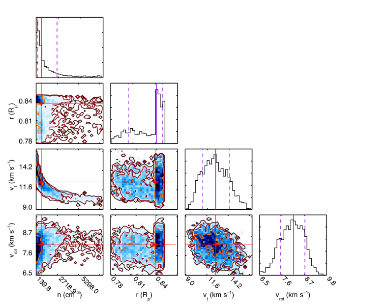
Figure 4: Posterior distributions and marginalized histograms for the atmosphere fits to the Balmer lines. The median values are marked on the posterior distributions with a red square and on the marginalized histograms with a purple line. The 68% confidence intervals for each parmeter are marked with dashed purple lines. The 68%, 95%, and 99% contours are also overplotted.

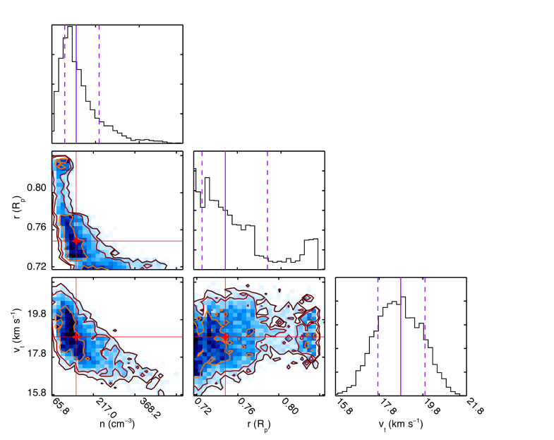
Figure 5: Posterior distributions and marginalized histograms for the atmosphere fits to the Balmer lines in the case of no rotation. The format is the same as Figure 4

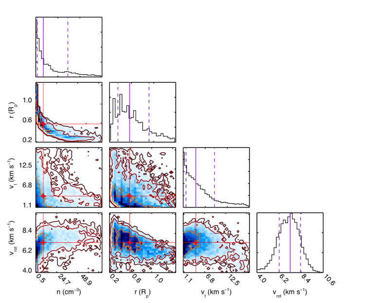
Figure 6: Same format as Figure 4 except for the Mg I lines. The density $n$ and radial atmospheric extent $r$ are directly correlated since the Mg I lines are optically thin, which allows a broad range of values for $n$ and $r$. Additional Mg I transitions are needed to better constrain the atmosphere probed by the Mg I optical triplet.

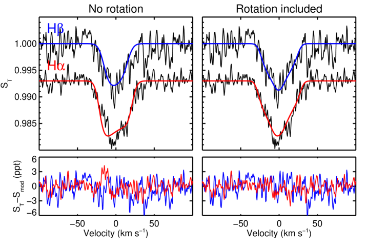
Figure 7: Best-fit Balmer line models for the case of no rotation (left panels) and including rotation (right panels). The fit residuals are shown in the bottom panels. The H$\alpha$ data is shown in black and the H$\beta$ data is shown in dark gray. The H$\alpha$ models are plotted as red lines; the H$\beta$ models as blue lines. The rotation model provides better fits to Balmer lines and has a substantially lower BIC value, indicating a statistically preferred model compared with the case of no rotation.

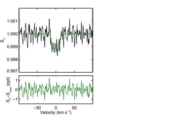
Figure 8: Best-fit atmospheric model to the Mg I line. Although non-zero rotation is preferred, the atmospheric parameters are highly uncertain and the in-transit variability calls into question the spherical symmetry assumed in the model.

Table 3: Best-fit atmospheric parameters

Parameter	Symbol	Units	Mg I	Balmer
Number density	$n$	cm-3	$10.0^{+31.9}_{-7.6}$	$836.0^{+2773.9}_{-487.8}$
Radial extent	$R_{\text{p}}+r$	$R_{\text{p}}$	$0.6^{+0.4}_{-0.2}$	$0.84^{+0.01}_{-0.04}$
Thermal broadening	$v_{\text{t}}$	km s-1	$4.4^{+5.9}_{-2.7}$	$12.6^{+1.8}_{-1.7}$
Rotational velocity	$v_{\text{rot}}$	km s-1	$7.4^{+1.1}_{-1.2}$	$8.2^{+0.6}_{-0.7}$

Including rotation in the atmospheric model results in a statistically better fit for the Balmer lines: we find a difference in the Bayesian information criterion (Schwarz 1978; Liddle 2007) of $\Delta\text{BIC}=76$ where the rotation model has the lower BIC. Since $\Delta\text{BIC}>10$ is generally considered decisive evidence in favor of the lower BIC model, we conclude that the model value of $v_{\text{rot}}=8.2^{+0.6}_{-0.7}$ km s^-1 is indeed tracing the planetary rotation. Although the Mg I model fits are less well constrained than the simultaneous fits to the Balmer lines, and may be contaminated by non-spherically symmetric atmospheric absorption, the value of $v_{\text{rot}}=7.4^{+1.1}_{-1.2}$ km s^-1 is consistent with the tidal-locked equatorial rotational velocity. The Balmer line value is suggestive of mild superrotation which may be the result of higher jet speeds at greater altitudes (e.g., Rauscher & Kempton 2014).

3.4 Absorption time series

We examine how the absorption in the various atomic species changes as a function of transit time. For the Balmer lines, the absorption is strong enough to consider the lines individually. The metal line depths are fairly shallow ($\approx 0.1-0.4$%) but there are at least two individual lines with significant absorption in the average transmission spectrum for each of the metal line species. We thus co-add the individual lines from each species to produce an average line profile at each observation time. This increases the S/N by a factor of $\approx\sqrt{N}$, where $N$ is the number of detected lines for that species. The absorption is calculated identically to the average in-transit values. To derive uncertainties for the individual time series points, we consider both the Poisson noise in the co-added spectrum and the standard deviation of the out-of-transit points used in the average out-of-transit spectrum. The larger of the two is conservatively used as the $1\sigma$ uncertainty for each point. In addition to the detected atomic species, we also perform the same time series procedure for the control region discussed in Section 3.2. This ensures that our analysis is not producing spurious absorption features. The individual in-transit spectra used to calculate the time series are given in Appendix A.

The metal time series are shown in Figure 9 and the Balmer line time series are shown in Figure 10. In both plots the transit contact points are marked with vertical gray lines. The time series absorption calculated with the favored Balmer line model from Section 3.3 is shown with solid lines in Figure 10. In Figure 9 the time series for the control region is shown in black in the bottom panel.

The timeseries show significant structure: most of the metal lines show initially weak absorption, increasing rather sharply towards mid-transit and then abruptly decreasing before third contact. The Balmer time series show very similar structure and are not well represented by the spherically symmetric atmosphere models from Section 3.3 (solid lines in Figure 10).

Strikingly, all of the lines show a marked emission-like feature immediately before third contact which disappears immediately after fourth contact. Since $S_{\text{T}}$ is a relative measurement of spectral lines observed at different times, emission features could also be the lack of absorption during one exposure compared with another. However, the stability of the out-of-transit points suggests that the emission bump is indeed a filling in of the nominal line core; a relative decrease in absorption would likely show a continuing trend during the out-of-transit exposures since these points would still be in absorption relative to the emission peak.

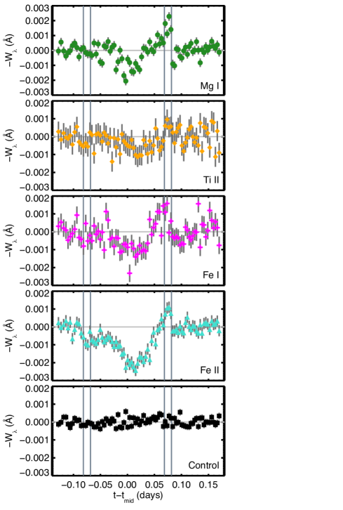
Figure 9: Timeseries absorption for average combined profiles of all the detected metal lines. The vertical gray lines mark the transit contact points and the horizontal gray line is at $-W_{\lambda}=0$. The legend is given in the lower right corner. There is significant structure in the light curves and the metal absorption tends to correlate across the various lines. The positive bump immediately before third contact is consistent across all lines and also appears in the Balmer line time series (see Figure 10).

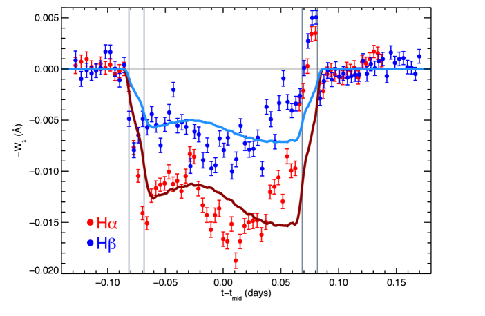
Figure 10: Timeseries of H$\alpha$ and H$\beta$ absorption. The favored atmosphere model time series is overplotted with the solid dark lines. Note the deviations from the symmetric atmosphere model and the emission feature near third contact, which is also evident in the metal line time series in Figure 9.

4 DISCUSSION

Here we discuss the atmospheric model line profiles and possible explanations for the origin of the in-transit absorption variability.

4.1 Atmospheric rotation

We showed that the Balmer line and Mg I average in-transit transmission spectra are well-fit with rotational velocities of $7.4^{+1.1}_{-1.2}$ km s^-1 and $8.2^{+0.6}_{-0.7}$ km s^-1, respectively. The Mg I value of $v_{\text{rot}}$ is consistent with KELT-9 b being tidally locked to its host. The Balmer line value, however, suggests that KELT-9 b is mildly supperotating. We do not take into account the effects of jets or day-to-nightside winds in KELT-9 b’s thermosphere, which should produce a bulk blue-shift in the transmission spectrum. These features naturally occur in hot planet atmospheres (e.g., Showman et al. 2008; Rauscher & Menou 2010) and have been marginally detected in HD 209458 b (Snellen et al. 2010) and HD 189733 b (Louden & Wheatley 2015). With the potential exception of H$\beta$, no significant net blue-shifts are seen in our spectra (see Table 2). However, as discussed in Section 3.3, velocities associated with the in-transit variability may mask the nominal atmospheric wind velocities.

The difference in the model $v_{\text{rot}}$ values may also be due to the different pressure regions probed by the Balmer lines compared with the Mg I triplet. Miller-Ricci Kempton & Rauscher (2012) showed that wind speeds of up to $\approx 15$ km s^-1 can form in atmospheres with no magnetic drag, at pressure consistent with the formation of the Balmer lines. Rotation combined with jet speeds of $\approx 2-3$ km s^-1 could be enough to explain the large $v_{\text{rot}}$ value for the Balmer lines. Future non-variable transits should provide cleaner opportunities to measure the normal atmospheric motions of KELT-9 b. Modeling efforts aimed at the optical Mg I triplet would also be helpful in breaking the degeneracy between the density and radial extent of the atmosphere.

4.2 Estimating the mass loss rate of KELT-9 b

Thermal atmospheric escape is predicted to be a ubiquitous phenomenon for hot gas giants (e.g., Murray-Clay et al. 2009; Salz et al. 2016) and has been calculated in a handful of systems using models of the high-velocity wings of Lyman-$\alpha$ (Vidal-Madjar et al. 2003; Lecavelier des Etangs et al. 2010; Ehrenreich et al. 2012; Kulow et al. 2014; Ehrenreich et al. 2015). Gaudi et al. (2017) estimated a mass loss rate of $\dot{M}\approx 10^{10}-10^{13}$ g s^-1. where the large range is due to uncertainty concerning KELT-9’s emitted non-thermal radiation and stellar activity level. Yan & Henning (2018) were able to use an analytic atmospheric model to derive a density based on their observed H$\alpha$ profile and estimate a mass loss rate of $\dot{M}\approx 10^{12}$ g s^-1.

We can use the densities derived from our atmospheric models to calculate an approximate mass loss rate for KELT-9 b. For the case of Mg I, the number density of the triplet ground state is $n=10.0$ cm^-3. We assume that the material is moving at $10$ km s^-1 as it passes through the model value $r=1.6R_{\text{p}}$. If we assume statistical equilibrium for the magnesium atoms and a thermospheric temperature of $T=10,000$ K, the ratio of Mg I triplet states to the Mg I ground state is $\approx 0.2$. If we further assume that half of all the magnesium atoms are ionized, we arrive at a total mass loss rate for magnesium of $\dot{M}_{MgI}\approx 3.6\times 10^{7}$ g s^-1. Finally, assuming a solar magnesium abundance for KELT-9 b (Asplund et al. 2009), we calculate an approximate total mass loss rate of $\dot{M}\approx 1\times 10^{12}$ g s^-1. Performing a similar exercise with the Balmer line atmospheric parameters, and assuming $n_{2}/n_{1}=10^{-6}$, we calculate $\dot{M}\approx 3\times 10^{12}$ g s^-1, similar to the Mg I value.

Mass loss calculations of this sort are highly uncertain due to assumptions concerning the level populations, outflow velocity, planetary abundances, and ionization state. However, it is encouraging that both of our estimates, which are based on the density and radial extent derived from atmospheric modeling, are within the range expected from energy deposition calculations and agree with the value from Yan & Henning (2018). Atmospheric models of ground-state Mg I absorption coupled with simultaneous observations of the excited state Mg I optical triplet could provide strict constraints on a planet’s mass loss rate.

4.3 In-transit absorption variability and the emission feature

Both the metal line and Balmer line time series display interesting sub-structure. This is most visible in the Balmer line absorption in Figure 10 but can also be clearly seen in the Fe II panel in Figure 9: the absorption is initially fairly weak and, in the case of the Balmer lines, appears to correspond to the symmetric atmosphere model and then begins to increase near mid-transit before sharply decreasing around $t-t_{\text{mid}}\approx 0.05$ days, i.e., the emission feature mentioned in Section 3.4.

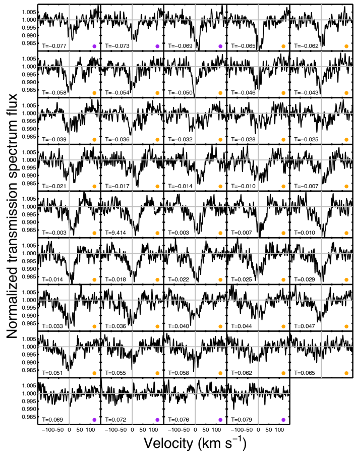
Figure 14: Individual in-transit transmission spectra of H$\alpha$. The format is the same as Figure 13.

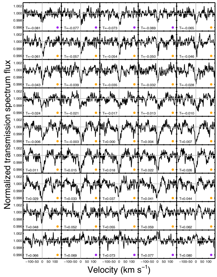
Figure 18: Individual in-transit transmission spectra of the combined Fe II line profile. The format is the same as Figure 13.

We can gain additional information by looking at the velocities of the transmission line profiles. Due to the low signal-to-noise of most of the metal lines, and some of the H$\beta$ lines, we focus on the the individual H$\alpha$ and Fe II profiles (see Figure 14 and Figure 18). The velocities, or what we will call $V_{0}$, are calculated as a flux-weighted average of the planetary-frame transmission spectrum between $\pm 50$ km s^-1. The uncertainties are the standard deviation of the velocities which contribute 68% of the transmission spectrum absorption or emission across the $\pm 50$ km s^-1 velocity range. Thus broader profiles have larger uncertainties compared with narrow profiles.

The in-transit H$\alpha$ and Fe II velocities are shown in Figure 11. Initially, $V_{0}$ is close to 0 km s^-1 for both lines, which is expected in the planet’s rest frame in the absence of other asymmetric velocity components. The velocities in both lines then become strongly red-shifted near $t-t_{\text{mid}}\approx-0.03$ days, similar to when the in-transit absorption increases. This occurs in both H$\alpha$ and Fe II, suggesting that both atomic populations are tracing similar regions in the atmosphere. Near $t-t_{\text{mid}}\approx 0.05$ days, when the emission features appear, the Fe II velocities become strongly red-shifted, due to the emission peaks in the spectra, and H$\alpha$ continues to be mildly blue-shifted, although most of the measurements are consistent with $V_{0}\approx 0.0$ km s^-1. The velocity variations cannot be caused by uncertainty in the planet’s orbital velocity: changing the in-transit line-of-sight velocity of the planet would leave a linear residual in the transmission profile velocities, not the non-uniform variations that are observed.

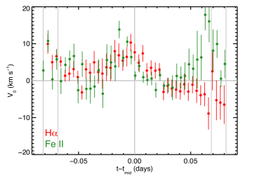
Figure 11: Flux-weighted velocity measurements $V_{0}$ for the individual H$\alpha$ and Fe II transmission spectra in Figure 14 and Figure 18. The vertical gray lines show the transit contact points and $t-t_{\text{mid}}=0.0$ days. The lines become red-shifted when the absorption increases around $t-t_{\text{mid}}\approx-0.03$ days and then gradually change to blue-shifted. The Fe II lines become sharply red-shifted when the emission features start to become prominent.

The metal and Balmer line timeseries exhibit a significant emission-like feature near third contact. Shown in Figure 12 are the average $S_{\text{T}}$ spectra for the Balmer lines, Mg I, and Fe II for times between third and fourth contact. There is remarkable consistency among the line profiles: blue-shifted absorption extending to $\approx 100$ km s^-1 and an emission peak that is red-shifted by $\approx 10$ km s^-1. The exception is H$\alpha$, which shows a weaker emission profile: two of the four spectra between third and fourth contact are in absorption, decreasing the emission strength. This is likely due to optical depth effects which prevent the absorption line core from being entirely filled in. We reiterate that the large blue-shifted velocities cannot be the result of uncertainty in the planet’s orbital velocity, which is at most $\approx 6-8$ km s^-1 (Gaudi et al. 2017; Yan & Henning 2018).

The profile shapes in Figure 12 are reminiscent of P-Cygni features, the result of strong stellar winds around luminous variable stars (e.g., Martins et al. 2015; Gillet et al. 2016) or accreting pre-main sequence stars (e.g., Edwards et al. 2003; Cauley & Johns-Krull 2014, 2015a). The blue-shifted absorption suggests a wind-like geometry where material is being accelerated away from the planet to velocities of $\approx 50-100$ km s^-1 in the direction of the observer. The P-Cygni profile disappears immediately after transit, constraining the geometry of the material to the immediate vicinity of the planet, i.e., a trailing tail of material would produce a post-transit absorption signature relative to the pre-transit observations.

Thermal expansion from the planet’s atmosphere alone cannot account for such large blue-shifted velocities (e.g., Trammell et al. 2014; Salz et al. 2016). Radiation pressure from the star is the only plausible mechanism capable of accelerating the planetary wind material to high velocities. Radiation pressure has been shown to strongly affect the geometry of planetary mass flows in other systems (e.g., Bourrier & Lecavelier des Etangs 2013; Bourrier et al. 2016; Spake et al. 2018).

Neglecting other forces, the ratio $\beta=F_{\text{rad}}/F_{\text{g}}^{\star}$, where $F_{\text{rad}}$ is the force due to radiation pressure on an atom and $F_{\text{g}}^{\star}$ is the stellar gravitational force, determines whether a particle at rest is pushed away ($\beta>1$) or falls towards the star ($\beta<1$). The value of $\beta$ for a particular atomic species is independent of the distance from the star since both $F_{\text{rad}}$ and $F_{\text{g}}^{\star}$ go like $r^{-2}$. Values of $\beta$ for some the atomic species of interest here have been calculated for systems similar to KELT-9: Beust et al. (2001) investigated the observational signatures of falling evaporating bodies around Herbig Ae/Be stars and calculated $\beta$ for Fe I, Fe II, and H I in the case of $T_{\text{eff}}=10500$ K, $M_{\star}=2.4M_{\odot}$, $R_{\star}=1.75R_{\odot}$, and log$g=4.0$. They find $\beta_{\text{FeII}}=46.4$, $\beta_{\text{FeI}}=90.9$, and $\beta_{\text{HI}}=0.43$. Although $\beta_{\text{HI}}<1$ suggests that radiation pressure is not sufficient to accelerate hydrogen atoms, the hydrogen escaping from KELT-9 b is, in addition to the thermal expansion velocity away from the planet, in orbit and thus even moderate additional radial forces are capable of pushing hydrogen to larger velocities.

If we adopt the Beust et al. (2001) $\beta$ values for the KELT-9 system, is radiation pressure capable of producing the $\approx 50-100$ km s^-1 blue-shifts seen in the line profiles? We assume that the only forces acting on the planetary material are the planetary gravity and radiation pressure. We ignore the stellar gravitational potential since $F_{\text{g}}^{\text{pl}}\approx 1.6\times F_{\text{g}}^{\star}$ and the felt centripetal acceleration on the particles, in the absence of perturbations, balances the stellar gravity. For KELT-9 b, $a_{\text{g}}^{\text{pl}}=0.020$ km s${}^{-2}=1.59a_{\text{g}}^{\star}$. For Fe II particles moving radially away along the star-planet line, the net acceleration is then $a_{\text{net}}\approx 0.56$ km s^-2 away from the planet. Under constant acceleration, an Fe II atom could reach velocities of $\approx 100$ km s^-1 in $\approx 3$ minutes.

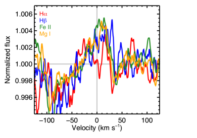
Figure 12: Average transmission spectra for H$\alpha$, H$\beta$, Mg I, and Fe II in the planetary rest frame for times between third and fourth contact where the emission peaks in Figure 9 and Figure 10. The spectra are smoothed by 10 pixels for clarity and the Fe II and Mg I spectra have been scaled to make them comparable in strength to the Balmer line spectra. The line profiles show P-Cygni-like shapes: red-shifted emission and blue-shifted absorption, indicative of outflowing material.

The above idealized calculation ignores self-shielding of the atmosphere, which reduces $\beta$ and thus the acceleration due to radiation pressure. It also ignores any initial velocity given to the particles by the planetary wind. Nonetheless, the order-of-magnitude estimates suggest that radiation is capable of producing the blue-shifted velocities seen in Figure 12. Note that the blue-shifted velocities in the line profiles in Figure 12 are outside of the velocity range used to calculate $V_{0}$ in Figure 11. Thus the values of $V_{0}$ between third and fourth contact are tracing the mildly red-shifted emission lines for Fe II. If the material is strongly accelerated radially away from the star-planet line, this could produce the geometry necessary to explain the disappearance of the absorption immediately after transit: a narrow cometary tail will form behind the planet with little azimuthal extent. This is similar to what is predicted for WASP-107 b based on the detection of He I 10830 Å (Oklopc̆ić & Hirata 2018; Spake et al. 2018).

The in-transit absorption and velocity variations are indicative of dynamic circumplanetary material or time variability in the density and structure of the extended atmosphere. Another possibility is that variations in stellar activity or the transiting of quiescent stellar active regions are affecting the transmission spectra. However, KELT-9 is an A0V/B9V star and it is unlikely that it has the active region coverage fraction or intrinsic active region contrast necessary to produce such changes in the Balmer lines via transits of bright active regions (Cauley et al. 2018). An increase in stellar brightness would cause a decrease in the transmission spectrum strength. Thus the in-transit variations are probably intrinsic to changes in the planet’s extended atmosphere.

We propose the following scenario to explain both the absorption increase near $t-t_{\text{mid}}\approx-0.03$ and the large blue-shifted velocities near the end of the transit: a stellar flare caused an inflation of the planet’s extended atmosphere and a spike in the mass loss rate, creating the enhanced absorption around $t-t_{\text{mid}}\approx-0.03$ days. The expanding material escaped and was accelerated away from the planet, which produces the P-Cygni line profiles.

Although the presence of flares on A-stars is debated (e.g., Balona 2015; Pedersen et al. 2017), we now know of spots (Böhm et al. 2015; Petit et al. 2017) and small-scale magnetic fields on normal A0V stars (e.g., Vega; Ligniéres et al. 2009; Petit et al. 2010). Thus it is not implausible that a small flare event, perhaps triggered by an interaction between the stellar and planetary magnetic fields (e.g., Lanza 2009; Strugarek et al. 2014), is responsible for the observed phenomena. Future spectroscopic transit observations with simultaneous photometry will help determine the origin of these features and quantify how common they are for this system.

5 SUMMARY AND CONCLUSIONS

We observed the transit of the ultra-hot Jupiter KELT-9 b using the high-resolution spectrograph PEPSI on the LBT. In addition to confirming the detections of Ti II, Fe I, Fe II, and H$\alpha$ in the atmosphere of KELT-9 b, we report the precense of H$\beta$ and the first detection of the optical Mg I triplet in an exoplanet atmosphere. Magnesium is an important coolant in exoplanet atmospheres (Huang et al. 2017) and may be a useful diagnostic of evaporation (Bourrier et al. 2015). Mass loss rates calculated from the Balmer line and Mg I atmospheric parameters agree well with previous estimates from Gaudi et al. (2017) and Yan & Henning (2018).

We reproduced the extended hydrogen envelope absorption with rotating atmosphere models and found that rotation velocities of $\approx 8$ km s^-1 are strongly preferred to the case of no rotation. This suggests that the Balmer lines trace a region of the atmosphere that is mildly superrotating compared with the tidally locked rotation rate. Models of the Mg I absorption suggest a rotation rate consistent with the planet being tidally locked, although the Mg I atmospheric model parameters are much more uncertain. The in-transit absorption variability likely complicates the line Mg I profile shape, with possible contributions to the profile velocity information from mass flows associated with evaporating material, making the precise interpretation of the rotational velocity difficult. Observations of a more uniform transit will allow for better constraints on the rotational information contained in the Mg I line profiles.

The time-resolved transit absorption shows significant variations in all of the detected atomic species, including the hydrogen Balmer lines, and suggests that the transiting planetary material is spatially non-uniform or varying in time. An emission feature at the end of the transit is suggestive of mass loss from the planet and shows spectroscopic features similar to strong stellar winds, evidence that the evaporating material is being rapidly accelerated away from the planet, likely by radiation pressure from the star. We suggest that the sudden in-transit absorption variability, and subsequent appearance of P-Cygni profiles in the transmission spectra, are evidence of a flaring event that resulted in enhanced mass loss and thus a larger extended atmosphere. More spectroscopic transits, combined with simultaneous photometry, are needed to determine the frequency of such behavior and help understand the physical cause of the in-transit variability.

Acknowledgments: P. W. C. and E. L. S. are grateful for support from NASA Origins of the Solar System grant No. NNX13AH79G (PI: E.L.S.). It is also our pleasure to thank the German Federal Ministry (BMBF) for the year-long support for LBT/PEPSI through their Verbundforschung with grants 05AL2BA1/3 and 05A08BAC. S. R. acknowledges support from the National Science Foundation through Astronomy and Astrophysics Research Grant AST-1313268. A. G. J. wishes to acknowledge support through NASA Exoplanet Research Program grant 14-XRP14-2-0090 to the University of Nebraska at Kearney. This work has made use of NASA’s Astrophysics Data System.

Appendix A Individual transmission spectra

In this appendix we show the in-transit spectra for each of the lines presented in Section 3. These line profiles are used to calculate the values shown in Figure 9 and Figure 10.

Figure 13: Individual in-transit transmission spectra of H$\beta$. The transit time in days from mid-transit is given in the lower left of each panel. Panels marked with a purple dot signify transit times between 1st and 2nd or 3rd and 4th contact; orange dots mark spectra taken between 2nd and 3rd contact, which are the spectra used to create the average in-transit profiles shown in Figure 2. All spectra are smoothed with a 5-pixel boxcar kernel for clarity.

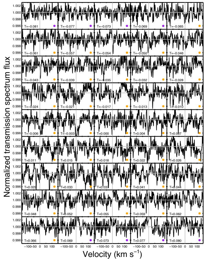
Figure 15: Individual in-transit transmission spectra of the combined Mg I line profile. The format is the same as Figure 13. Note the Fe II 5169.0 Å line near $+100$ km s^-1.

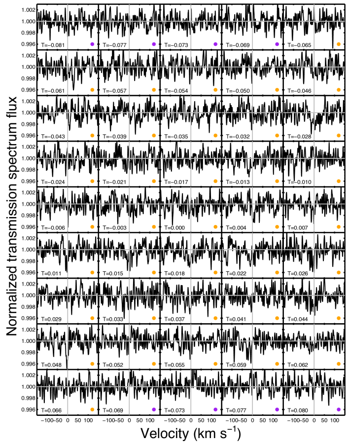
Figure 16: Individual in-transit transmission spectra of the combined Ti II line profile. The format is the same as Figure 13.

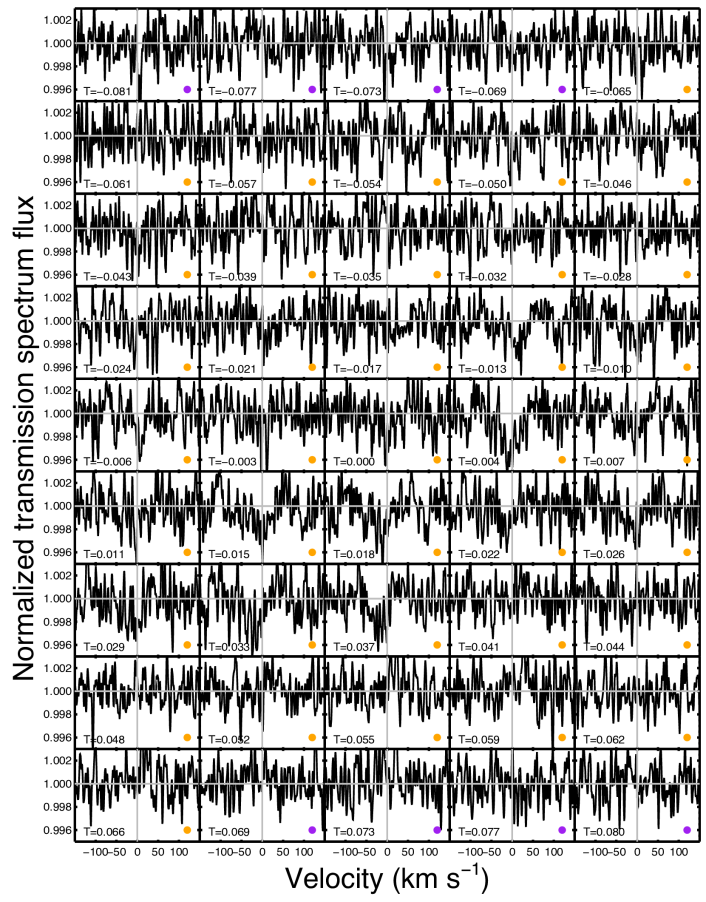
Figure 17: Individual in-transit transmission spectra of the combined Fe I line profile. The format is the same as Figure 13.

References

- Asplund et al. (2009) Asplund, M., Grevesse, N., Sauval, A. J., & Scott, P. 2009, ARAA, 47, 481
- Balona (2015) Balona, L. A. 2015, MNRAS, 447, 2714
- Beust et al. (2001) Beust, H., Karmann, C., & Lagrange, A.-M. 2001, A&A, 366, 945
- Böhm et al. (2015) Böhm, T., Holschneider, M., Ligniéres, F., et al. 2015, A&A, 577, A64
- Bourrier & Lecavelier des Etangs (2013) Bourrier, V., & Lecavelier des Etangs, A. 2013, A&A, 557, A124
- Bourrier et al. (2015) Bourrier, V., Lecavelier des Etangs, A., & Vidal-Madjar, A. 2015, A&A, 573, A11
- Bourrier et al. (2016) Bourrier, V., Lecavelier des Etangs, A., Ehrenreich, D., Tanaka, Y. A., & Vidotto, A. A. 2016, A&A, 591, A121
- Brogi et al. (2016) Brogi, M., de Kok, R. J., Albrecht, S., et al. 2016, ApJ, 817, 106
- Casasayas-Barris et al. (2017) Casasayas-Barris, N., Palle, E., Nowak, G., et al. 2017, A&A, 608, A135
- Casasayas-Barris et al. (2018) Casasayas-Barris, N., Palle, E., Yan, F., Chen, G., et al. 2018, A&A, 616, A151
- Cauley & Johns-Krull (2014) Cauley, P. W., & Johns-Krull, C. M. 2014, ApJ, 797, 112
- Cauley & Johns-Krull (2015a) Cauley, P. W., & Johns-Krull, C. M. 2015, ApJ, 810, 5
- Cauley et al. (2015) Cauley, P. W., Redfield, S., Jensen, A. G., et al. 2015, ApJ, 810, 13
- Cauley et al. (2017a) Cauley, P. W., Redfield, S., & Jensen, A. G. 2017, AJ, 153, 217
- Cauley et al. (2018) Cauley, P. W., Kuckein, C., Redfield, S., et al. 2018, AJ, in press (https://arxiv.org/abs/1808.09558)
- Cauley et al. (2018a) Cauley, P. W., Shkolnik, E. L., Llama, J., Bourrier, V., & Moutou, C. 2018, AJ, in press
- Cauley et al. (2018b) Cauley, P. W., Shkolnik, E. L., & Llama, J. 2018, RNAAS, 2, 23
- Chen et al. (2018) Chen, G., Pallé, E., Welbanks, L., et al. 2018, A&A, 616, A145
- Christie et al. (2013) Christie, D., Arras, P., & Li, Z.-Y. 2013, ApJ, 772, 144
- Cuntz et al. (2000) Cuntz, M., Saar, S. H., & Musielak, Z. E. 2000, ApJ, 533, L151
- Czesla et al. (2015) Czesla, S., Klocová, T., Khalafinejad, S., Wolter, U., & Schmitt, J. H. M. M. 2015, A&A, 582, A51
- Deming et al. (2013) Deming, D., Wilkins, A., McCullough, P., et al. 2013, ApJ, 774, 95
- Edwards et al. (2003) Edwards, S., Fischer, W., Kwan, J., Hillenbrand, L., & Dupree, A. K. 2003, ApJ, 599, L41
- Ehrenreich et al. (2012) Ehrenreich, D., Bourrier, V., Bonfils, X., et al. 2012, A&A, 547, A18
- Ehrenreich et al. (2015) Ehrenreich, D., Bourrier, V., Wheatley, P. J., et al. 2015, Nature, 522, 459
- Foreman-Mackey et al. (2012) Foreman-Mackey, D., Hogg, D. W., Lang, D., & Goodman, J. 2012, arXiv:1202.3665
- Fossati et al. (2010) Fossati, L., Haswell, C. A., Froning, C. S., et al. 2010, ApJ, 714, L222
- Gaudi et al. (2017) Gaudi, S., Stassun, K. G., Collins, K. A., et al. 2017, Nature, 546, 514
- Gillet et al. (2016) Gillet, D. Sefyani, F. L., Benhida, A., et al. 2016, A&A, 587, A134
- Goodman & Weare (2010) Goodman, J., & Weare, J. 2010, CAMCS, 5, 65
- Heng et al. (2015) Heng, K., Wyttenbach, A., Lavie, B., et al. 2015, ApJ, 803, 9
- Hoeijmakers et al. (2018) Hoeijmakers, H. J., Ehrenreich, D., Heng, K., et al. 2018, Nature, 560, 453
- Huang et al. (2017) Huang, C., Arras, P., Christie, D., & Li, Z.-Y. 2017, submitted to ApJ
- Jensen et al. (2011) Jensen, A. G., Redfield, S., Endl, M., et al. 2011, ApJ, 743, 203
- Jensen et al. (2012) Jensen, A. G., Redfield, S., & Endl, M., et al. 2012, ApJ, 751, 86
- Jensen et al. (2018) Jensen, A. G., Cauley, P. W., Redfield, S., Cochran, W. D., & Endl, M. 2018, AJ, 156,154
- Kausch et al. (2015) Kausch, W., Noll, S., Smette, A., et al. 2015, A&A, 576, A78
- Khalafinejad et al. (2017) Khalafinejad, S., von Essen, C., Hoeijmakers, H. J., et al. 2017, A&A, 598, A131
- Kitzmann et al. (2018) Kitzmann, D., Heng, K., Rimmer, P. B., et al. 2018, ApJ, 863, 183
- Knutson et al. (2007) Knutson, H. A., Charbonneau, D., Noyes, R. W., Brown, T. M., & Gilliland, R. L. 2007, ApJ, 655, 564
- Knutson et al. (2014) Knutson, H. A., Benneke, B., Deming, D., & Homeier, D. 2014, Nature, 505, 66
- Kreidberg et al. (2015) Kreidberg, L., Line, M. R., Bean, J. L., et al. 2015, ApJ, 814, 66
- Kreidberg et al. (2018) Kreidberg, L., Line, M. R., Thorngren, D., Morley, C. V., & Stevenson, K. B. 2018, ApJ, 858, 6
- Kulow et al. (2014) Kulow, J. R., France, K., Linsky, J., & Loyd, R. O. P. 2014, ApJ, 786, 132
- Lanza (2009) Lanza, A. F. 2009, A&A, 505, 339
- Lecavelier des Etangs et al. (2010) Lecavelier des Etangs, A., Ehrenreich, D., Vidal-Madjar, A., et al. 2010, A&A, 514, A72
- Lecavelier des Etangs et al. (2012) Lecavelier des Etangs, A., Bourrier, A., Wheatley, P. J., et al. 2012, A&A, 543, L4
- Liddle (2007) Liddle, A. R. 2007, MNRAS, 377, L74
- Ligniéres et al. (2009) Ligniéres, F., Petit, P., Böhm, T., & Auriére, M. 2009, A&A, 500, 41
- Llama et al. (2011) Llama, J., Wood, K., Jardine, M. et al., 2011, MNRAS, 416, L41
- Llama et al. (2013) Llama, J., Vidotto, A. A., Jardine, M., et al. 2013, MNRAS, 436, 2179
- Louden & Wheatley (2015) Louden, T., & Wheatley, P. J. 2015, ApJL, 814, L24
- Mallonn & Strassmeier (2016) Mallonn, M., & Strassmeier, K. G. 2016, A&A, 590, A100
- Mansfield et al. (2018) Mansfield, M., Bean, J. L., Oklopc̆ić, A., et al. 2018, ApJL, 868, L34
- Martins et al. (2015) Martins, F., Marcolino, W., Hillier, D. J., Donati, J.-F., & Bouret,J.-C. 2015, A&A, 574, A142
- Miller-Ricci Kempton & Rauscher (2012) Miller-Ricci Kempton, E., & Rauscher, E. 2012, ApJ, 751, 117
- Murray-Clay et al. (2009) Murray-Clay, R. A., Chiang, E. I., & Murray, N. 2009, ApJ, 693, 23
- Oklopc̆ić & Hirata (2018) Oklopc̆ić, A., & Hirata, C. M. 2018, ApJ, 855, 11
- Owen & Jackson (2012) Owen, J. E., & Jackson, A. P. 2012, MNRAS, 425, 2931
- Pedersen et al. (2017) Pedersen, M. G., Antoci, V., Korhonen, H., et al. 2017, MNRAS, 466, 3060
- Petit et al. (2010) Petit, P., Ligniéres, F., Wade, G. A., et al. 2010, A&A, 523, 41
- Petit et al. (2017) Petit, P., Hébrard, E. M., Böhm, T., Folsom, C. P., & Ligniéres, F. 2017, MNRAS, 466, 3060
- Piskunov & Valenti (2017) Piskunov, N., & Valenti, J. A. 2017, A&A, 597, A16
- Pont et al. (2013) Pont, F., Sing, D. K., Gibson, N. P., et al. 2013, MNRAS, 432, 2917
- Rauscher & Menou (2010) Rauscher, E., & Menou, K. 2010, ApJ, 714, 1334
- Rauscher & Kempton (2014) Rauscher, E., & Kempton, E. M. R. 2014, ApJ, 790, 79
- Redfield et al. (2008) Redfield, S., Endl, M., Cochran, W. D., & Koesterke, L. 2008, ApJ, 673, L87
- Salz et al. (2016) Salz, M., Czesla, S., Schneider, P. C., & Schmitt, J. H. M. M. 2016, A&A, 586, A75
- Schwarz (1978) Schwarz, G. 1978, Ann. Statist., 5, 461
- Shkolnik et al. (2005) Shkolnik, E., Walker, G. A. H., Bohlender, D. A., Gu, P.-G., & Kürster, M. 2005, ApJ, 622, 1075
- Shkolnik et al. (2008) Shkolnik, E., Bohlender, D. A., Walker, G. A. H., & Collier Cameron, A. 2008, ApJ, 676, 628
- Showman et al. (2008) Showman, A. P., Cooper, C. S., Fortney, J. J., & Marley, M. S. 2008, ApJ, 682, 559
- Sing et al. (2016) Sing, D. K., Fortney, J. J., Nikolov, N., et al. 2016, Nature, 529, 59
- Smette et al. (2015) Smette, A., Sana, H., Noll, S., et al. 2015, A&A, 576, A77
- Snellen et al. (2008) Snellen, I. A. G., Albrecht, S., de Mooij, E. J. W., & Le Poole, R. S. 2008, A&A, 487, 357
- Snellen et al. (2010) Snellen, I. A. G., de Kok, R. J., de Mooij, E. J. W., & Albrecht, S. 2010, Nature, 465, 1049
- Spake et al. (2018) Spake, J. J., Sing, D. K., Evans, T. M., et al. 2018, Nature, 557, 68
- Strassmeier et al. (2015) Strassmeier, K. G., Ilyin, I., Järvinen, A., et al. 2015, AN, 336, 324
- Strassmeier et al. (2018) Strassmeier, K. G., Ilyin, I., Steffen, M. 2018, A&A, 612, A44
- Strugarek et al. (2014) Strugarek, A., Brun, A. S., Matt, S. P., & Réville, V. 2014, ApJ, 795, 86
- Trammell et al. (2014) Trammell, G. B., Zhi-Yun, L., & Arras, P. 2014, ApJ, 788, 161
- Valenti & Piskunov (1996) Valenti, J. A., & Piskunov, N. 1996, A&ASS, 118, 595
- Vidal-Madjar et al. (2003) Vidal-Madjar, A., Lecavelier des Etangs, A., Désert, J.-M., et al. 2003, Nature, 422, 143
- Vidotto et al. (2010) Vidotto, A. A., Jardine, M., & Helling, Ch. 2010, ApJ, 722, L168
- Wilson et al. (2015) Wilson, P. A., Sing, D. K., Nikolov, N., et al. 2015, MNRAS, 450, 192
- Wyttenbach et al. (2015) Wyttenbach, A., Ehrenreich, D., Lovis, C., Udry, S., & Pepe, F. 2015, A&A, 577, A62
- Wyttenbach et al. (2017) Wyttenbach, A., Lovis, C., Ehrenreich, D., et al. 2017, A&A, 602, A36
- Yan et al. (2015) Yan, F., Fosbury, R. A. E., Petr-Gozens, M. G., Zhao, G., & Pallé, E. 2015, A&A, 574, A94
- Yan et al. (2017) Yan, F., Pallé, E., Fosbury, R. A. E, Petr-Gozens, M. G., & Henning, Th. 2017, A&A, 603, A73
- Yan & Henning (2018) Yan, F., & Henning, T. 2018, Nature Astronomy, 2, 714