Abstract

For the two-mode and $(N-1)-$bosonic Bose-Hubbard quantum system a less usual phase transition controlled by the parameter $\varepsilon$ representing the on-site energy difference is studied. In the literature the parameter is considered either real ($\varepsilon>0$) or purely imaginary (with, say, $\gamma={\rm Im}\ \varepsilon>0$), so the phase transition is analyzed here at the interface $\varepsilon=\gamma=0$. The evolution in the $\gamma-$controlled phase is required unitary so that the main task for the theory is found in the (quasi-)Hermitization of the Hamiltonian, achieved by a suitable amendment of the inner product in Hilbert space, $\langle\cdot|\cdot\rangle\to\langle\cdot|\Theta|\cdot\rangle$. In the most relevant domain of small $\gamma$ the linearized Hilbert-space metric $\Theta(\gamma)$ (constrained by the requirement $\lim_{\gamma\to 0}\Theta(\gamma)=I$ of the smoothness of the change of the Hilbert space at the phase transition) is constructed in closed form. Beyond the phase-transition instant, several forms of the systematic non-numerical recurrent construction of the exact metrics $\Theta(\gamma)$ are also shown user-friendly and feasible, at the not too large matric dimensions $N$ at least.

Keywords

quantum phase transitions; Bose-Hubbard model; non-Hermitian ${\cal PT}-$symmetric phase; unitary evolution; ad hoc  Hilbert-space metrics; non-numerical construction methods;

1 Introduction

Bosonic version of the Hubbard model is called Bose-Hubbard model [1]. It describes the zero-spin particles on a lattice at zero temperature in a way which is well adapted, in the context of solid state physics, to the study of the phase transition between its superfluid and insulator phases induced by the variation of the density [2]. In the conventional many-body setting the Bose-Hubbard (BH) Hamiltonian is, typically, able to deal with the Bose-Einstein condensation [3]. The amendments of the model can also offer a theoretical background to various other forms of the quantum phase transitions, say, in optical lattices [4].

The well known user-friendly mathematical tractability of the model [5] can be perceived as originating from its Lie-algebraic background. Thus, one can write the two-mode version of the conventional self-adjoint BH Hamiltonian in terms of the two angular-momentum generators $L_{x,z}$ of Lie algebra $su(2)$ using just three real parameters $\varepsilon,v$ and $c$ [6],

$$\mathfrak{h}_{(BH)}(\varepsilon,v,c)=2\varepsilon\,L_{z}+2v\,L_{x}+2c\,L^{2}_{z}=\mathfrak{h}^{\dagger}_{(BH)}(\varepsilon,v,c)\,.$$ (1)

Obviously, the most efficient treatment of the changes caused by the variations of the physical quantity $2c$ representing the strength of the interbosonic interactions will be provided by perturbation theory. Still, even if we restrict attention to the zero-order approximation, we are left with the variability of the two independent parameters, viz., of the quantity $2v$ which measures the intensity of the single-particle tunneling, and of the value $2\varepsilon$ which characterizes the bosonic on-site energy difference. One of these quantitites may be fixed via a suitable choice of the units. Thus, once we set, say, $v=1$, we only have to study the one-parametric problem.

In such a setting the authors of Refs. [6, 7] imagined that it is far from obvious that the parameter in question must be real. They gave several tenable arguments supporting the study of the possible inclusion of non-Hermiticities. In particular, the authors of Ref. [6] proposed the replacement of the bosonic on-site energy by a purely imaginary quantity,

$$2\varepsilon\to 2{\rm i}\gamma\,.$$ (2)

Naturally, the change opened a Pandora’s box of interpretational challenges. The main one was that the new, complexified Bose-Hubbard (CBH) Hamiltonian ceased to be a self-adjoint operator,

$$H_{(CBH)}(\gamma,v,c)=-2\,{\rm i}\gamma\,L_{z}+2v\,L_{x}+2c\,L^{2}_{z}\ \neq\ H_{(CBH)}^{\dagger}(\gamma,v,c)\,.$$ (3)

In  [6] the problem has been settled by an open-quantum-system upgrade of the underlying physics. In essence, an ad hoc  external field has been assumed to mimic the influence of the environment causing the parameter-controlled gains and/or losses of the bosons.

The authors of the idea felt inspired by the recent growth of interest in the Hamiltonians which are non-self-adjoint but ${\cal PT}-$symmetric (cf., e.g., reviews [8, 9, 10]). On this background it was possible to conclude that in the CBH model one can clearly distinguish between its “stable” and “unstable”dynamical regimes, separated by a new form of phase transition. In the former case, indeed, all of the eigen-energies remain real because the ${\cal PT}-$symmetry of the system is observed not only by the Hamiltonian but also by its eigen-states. In the “unstable” case, on the contrary, the ${\cal PT}-$symmetry becomes spontaneously broken. This means that some of the energies complexify while the related eigen-states cease to be ${\cal PT}-$symmetric.

The CBH-related research found one of its central topics in the study of the “instants” of the breakdown of ${\cal PT}-$symmetry. The existence of such “exceptional points” (EP) in the analytic quantum Hamiltonians is well know to mathematicians [11]. Still, the occurrence and the role of EPs in various physical systems has only been clarified rather recently [12]. In particular, the careful localization of the EP singularities $\gamma^{(EP)}_{(CBH)}(v,c)$ helped the authors of Ref. [6] to clarify further the connection between the CBH Hamiltonians (3) and the Bose-Einstein condensation.

In [13] we pointed out that besides the CBH class of the phenomenological models it is also possible to construct and use their various complex-symmetric $N$ by $N$ matrix generalizations for the same phenomenological purposes and in the same EP-related context. We concluded that one of the most characteristic physical features of any  Hamiltonian of the EP-supporting type is that in the apparently most interesting EP-controlled dynamical regime in which the system can perform a quantum phase transition the operator itself is strongly  non-Hermitian [14]. This leads to a rather paradoxical situation in which the study of the weakly  non-Hermitian regime (which is closer to the conventional Hermitian regime) is almost completely neglected in the literature. Now we intend to fill the gap. On an entirely abstract conceptual level such a project is promising because the popular restriction of attention to the strongly non-Hermitian EP-related quantum phase transitions is unnecessarily restrictive [15]. Here, we shall accept a different, less restrictive philosophy.

Our present project is inspired by our methodological study [16] in which a new model-building strategy has been outlined. In essence, we described there the new type of an EP-unrelated quantum phase transition using just a weak-non-Hermiticity mathematical background. Our return to this subject was recently re-encouraged when we noticed that the phenomenon of the EP-unrelated quantum phase transition was also revealed and predicted in several non-Hermitian multidimensional-oscillator examples [17] as well as in the realistic-physics context of the dissipative photonic systems [18] and/or, on experimental level of classical-physics simulations, of synthetic circuits [19].

In [16] our specific interface-passage considerations were illustrated by a schematic two-by-two matrix Hamiltonian. We in fact did not pay too much attention to the details of the evolution after  the passage. We were aware that a realistic illustration would be highly desirable and that such an illustration might have been provided by the CBH Hamiltonians (3). Still, we felt that the task might be prohibitively complicated, especially because after the passage the consistent description of the stable evolution of the system in question would necessarily  require the explicit  construction of the so called operator of charge [8] or, in a more general quasi-Hermitian setting of Refs. [20, 21], of the so called Hilbert-space metric $\Theta$.

Only recently, having reread section # 3 of paper [6] we imagined that a compromising solution might have been sought, and the purpose could have been served, by the simplified, unperturbed CBH model with $c=0$. The idea proved productive and it led to the results presented in what follows. Their presentation will be preceded by section 2 in which the reader finds a compact outline of the current stage of development of the concept of quantum phase transition, with special emphasis upon its non-Hermitian descriptions. In subsequent section 3 we shall describe the necessary technical aspects of the CBH model in its separate finite-dimensional $N$ by $N$ matrix representations. In particular, we shall point out that the consistent presentation of the model necessitates, via the construction of $\Theta_{(CBH)}$, the explicit  specification of the “standard” physical Hilbert space ${\cal H}^{(S)}_{(CBH)}$ in which one only can clarify the notion of the observability [9].

It is worth re-emphasizing that we will treat the CBH Hamiltonian (3) (with $c=0$) as the quasi-Hermitian operator [20, 22], i.e., as the generator of the evolution which is unitary in ${\cal H}^{(S)}$. In contrast to the open-system theories [23], our present version of the CBH model will be built differently, as a closed quantum system without any implicit or explicit reference to an interaction with the environment. The feasibility of such a project will be facilitated by the solvability of the model guaranteeing the reality (i.e., the potential observability) of the spectrum in a sufficiently large interval of $\gamma\in(0,\gamma_{\max})$.

As we already indicated, our main (and, in practice, almost always most difficult) technical task will be the construction of the after-the-transition Hamiltonian-dependent Hilbert space ${\cal H}^{(S)}={\cal H}^{(S)}_{(CBH)}(\gamma)$ or, more precisely, of its acceptable physical inner product. This will be done in section 4 (for the first nontrivial choice of $N=3$), in section 5 (for $N=4$) and in section 6 [where we will discuss the extrapolation of our knowledge to all $N$, with tests performed at $N=5$ (in subsection 6.1) and $N=6$ (in 6.2)]. Finally, our message will be summarized in section 7.

2 Hermitian - quasi-Hermitian phase transition

2.1 Analytic Hamiltonians and phase transitions at exceptional points

During the study of the phenomena called quantum phase transitions one might often hesitate whether certain abrupt changes of properties of a given system should still be given the name of phase transition. One not always finds a guidance in parallels between the classical and quantum physics [24]. In one direction, for a given quantum model it is not always easy to deduce the classical $\hbar\to 0$ limit. The situation is even worse in the opposite direction in which the correspondence principle leads to quantization recipes which may be ambiguous [25].

Examples of the incompleteness of the parallels abound, especially after the physics community accepted the idea that it may be useful to study stable quantum systems in their non-Hermitian (usually called ${\cal PT}-$symmetric alias  pseudo-Hermitian) representations (cf., e.g., the respective comprehensive reviews [8] and [9]). In such a framework several new theoretical ideas emerged during the last 25 years (cf., e.g., the introductory chapter in Ref. [10]). In 1992, for example, the well known, exactly solvable $N-$fermion Lipkin-Meshkov-Glick model of Ref. [26] has been generalized, by Scholtz et al [20], in a way which sampled, in the context of many-particle quantum physics, several new forms of phase transitions. Between 1997 and 1998 Bender with coauthors [27, 28] discovered, in a different context of quantum field theory, an equally interesting class of innovative quantum phase transitions which they called the spontaneous breakdown of ${\cal PT}$ symmetry.

These discoveries were followed by the identification of several quantum phase transition phenomena reflecting the presence of the Kato’s exceptional point (EP, [11]) in the Hamiltonian. In the most frequently encountered phase transition of this type the energies become complex so that the physical interpretation of the original, unitarily evolving and stable quantum system was lost. For the similar situations it is characteristic that one must introduce some new degrees of freedom so that the initial Hamiltonian $\Lambda_{0}^{(before)}$ as well as at least some of the other observables $\Lambda_{1}^{(before)},\Lambda_{2}^{(before)},\ldots$ must be replaced, after the passage of the system in question through its EP singularity, by some entirely different operators $\Lambda_{j}^{(after)}$ with $j=0,1,\ldots$.

In general, the description of the latter (also known as “‘first kind”) quantum phase transition requires also the change of the underlying physical Hilbert space, ${\cal H}^{(before)}\to{\cal H}^{(after)}$. Still, for some rather special quantum systems there also exist exceptions. In these cases one can admit the survival of kinematics (with ${\cal H}^{(before)}\equiv{\cal H}^{(after)}$) as well as of the dynamics (controlled by the same, EP-possessing and unchanged non-Hermitian Hamiltonian). This scenario (called “quantum phase transition of the second kind”, cf. [15]) is characterized by the mere partial  loss of the observability involving just a subset  of all of the relevant $\Lambda_{j}$s with $j\neq 0$.

In the latter scenario the evolution may be required to remain unitary. This is rendered possible by the fact that after the phase transition the bound-state energies are still real and observable. Nevertheless, as long as the change always involves at least some of the $j>0$ observables $\Lambda_{j}^{(before)}$, one encounters a full freedom in the choice of their descendants $\Lambda_{j}^{(after)}$. As a consequence, the change of operators $\Lambda_{j}^{(before)}\to\Lambda_{j}^{(after)}$ (which are all, under our overall unitary-evolution hypothesis, necessarily  quasi-Hermitian [20]) may imply, in general, a parallel consistent change of the metric operator, $\Theta^{(before)}\neq\Theta^{(after)}$. An analogous scenario will be also used and built in our present paper.

2.2 The instant of onset of non-Hermiticity

In the toy-model of Ref. [16] the conventional Hermiticity of observables was lost and replaced, at an ad hoc  phase-transition interface, by the so-called quasi-Hermiticity. Several features of the passage of the system through such a boundary were discussed, with emphasis upon the methodological aspects of the problem. The passage from the Hermitian to quasi-Hermitian dynamical regime was illustrated by the most elementary two-by-two-matrix toy model. Our Hamiltonian $H$ was time-dependent and non-Hermitian but ${\cal PT}-$symmetric, with real spectrum. Its elementary nature helped us to clarify the basic features of the mathematically correct treatment of the dynamics of the system. The question of a more realistic physical applicability of the formalism remained open.

Let us now return to Eq. (3) representing one of the most interesting non-Hermitian but still deeply realistic Hamiltonians. In subsequent sections we shall review some of the basic properties of the model, emphasizing the difference between its two possible physical probabilistic interpretations. We shall explain that in a way outlined in Refs. [23] and [9] this difference reflects the freedom of the choice between the non-unitarity and unitarity of the evolution or between the theoretical framework of the open and closed quantum system, respectively.

We shall restrict our attention to the unitary case. It has an advantage that our knowledge of the dynamics is complete, not involving any hypothetical environment. Due to the “hidden” form of the Hermiticity of the observables the dynamical information about the evolution may be carried not only by the Hamiltonian but also by the above-mentioned operator $\Theta$. Indeed, the latter Hilbert-space-metric operator carries such an information because it determines the correct physical inner product in the standard Hilbert space ${\cal H}^{(S)}$ [29].

Needless to add that in many models a guarantee of the compatibility between the information carried by $H$ and $\Theta$ can be nontrivial [30]. In fact, the necessity of this guarantee has been perceived, in the past, as one of the key obstructions of the applicability of the pseudo-Hermitian alias  ${\cal PT}-$symmetric constructions in realistic situations.

2.3 Non-Hermitian phase and the unitarity of its evolution

The authors of paper [6] circumvented the search for the Hilbert space ${\cal H}^{(S)}$ via the open-system physical treatment of their manifestly non-Hermitian quantum CBH Hamiltonians. They only studied the localization of the spontaneous breakdown of ${\cal PT}-$symmetry in the strongly non-Hermitian dynamical regime. In this case, the parameter $\gamma$ measuring the strength of the non-Hermiticity was assumed large, close to its maximal, transition-responsible EP value $\gamma^{(EP)}$.

Incidentally, we should add that even in the latter, truly extreme dynamical regime it should still be possible to follow the unitary-evolution philosophy and constructions, in principle at least. In practice one can of course expect that these constructions will be perceivably easier in the weakly non-Hermitian regime.

In the latter regime the main phenomenological advantages of the closed-system approach are twofold. Firstly, the unitary picture of the evolution generated by matrices $H^{(N)}_{(CBH)}(\gamma)$ is complete. There is no need of referring to an unspecified environment [31]. In ${\cal H}^{(S)}$ the underlying quantum theory becomes fully compatible with the conventional textbooks [32]. Secondly, the conservation of the unitarity during the non-EP phase transitions may open the way towards a matching of two alternative Hilbert-space representations of quantum world in a unified picture.

The replacement (2) may acquire, in this spirit, a smooth-transition meaning at an interface where $\varepsilon=\gamma=0$. For the sake of definiteness let us agree that we shall follow the very slow adiabatic change of the initially Hermitian BH model (1) in the limit of vanishing small $\varepsilon\to 0$. After the system touches the interface and after it performs the Hermiticity - non-Hermiticity phase transition (2), the subsequent evolution will be controlled by the complexified model (3), with a small $\gamma$, i.e., with the small imaginary  on-site energy difference.

In the new regime one must discuss several mathematical components of the model requiring, e.g., the reality of the energies and, secondly, a phenomenologically sufficiently well motivated choice of the correct physical Hilbert space. The latter process involves not only an explicit and correct constructive assignment of the metric $\Theta=\Theta(H)$ to the preselected Hamiltonian $H$ but also an appropriate suppression of the ambiguity of such an assignment (cf., e.g., [33] for an eligible “minimality” criterion and technique of such a suppression).

3 Hermitian vs. quasi-Hermitian Bose-Hubbard model

3.1 The matching at $\varepsilon=\gamma=0$

After the introductory considerations let us now turn attention back to the exactly solvable interaction-free (i.e., $c=0$) Bose-Hubbard model in its versions (1) and (3). No special remarks have to be added to the former case which is an entirely conventional Hermitian model. In our present notation it will be assigned, at any value of its real variable parameter $\varepsilon\geq 0$, the trivial metric $\Theta_{Hermitian}=I$.

Once we intend to speak about the Hermiticity/quasi-Hermiticity quantum phase transition in the limit $\varepsilon\to 0$ (i.e., say, at time $t=0$), we only have to describe the post-transition quantum system using the elementary complex upgrade (2) of the parameter at any $t>0$. The unitarity of the $t>0$ evolution may be then guaranteed by the proper interpretation of Schrödinger equation in an adiabatic approximation [34], i.e., for the sufficiently small times and $\gamma$s at least [35]. Our upgraded quasi-Hermitian Bose-Hubbard Hamiltonian (3) will be, subsequently, assigned a nontrivial metric $\Theta=\Theta(H)$.

The resulting pair of operators $H_{(CBH)}(\gamma)$ and $\Theta_{(CBH)}(\gamma)$ describing the dynamics after $t=0$ must necessarily satisfy the Dieudonné’s constraint

$$H^{\dagger}\Theta=\Theta H\,.$$ (4)

In what follows we intend to satisfy such a requirement constructively. Our construction will be facilitated by the knowledge of some basic properties of operators $H_{(CBH)}(\gamma)$ as provided by the authors of paper [6]. As long as they did not pay attention to the construction of $\Theta_{(CBH)}(\gamma)$, we will have to address the following questions:

• we will have to solve Dieudonné’s Eq. (4) interpreted as an implicit definition of metric;

• as long as the latter definition is ambiguous [36], we will restrict the class of solutions to the subclass of the candidates for metric which are positive definite;

• we will have to reduce the resulting set of eligible metrics $\Theta=\Theta_{j}(\gamma)$ to such a sub-family $\Theta_{j}^{(0)}(\gamma)$ for which the phase transition at $t=0$ would be smooth, i.e., for which the metric candidate trivializes in the limit $\gamma\to 0^{+}$, i.e.,

  $$\lim_{\gamma\to 0^{+}}\Theta_{j}^{(0)}(\gamma)=I\,;$$ (5)

• subsequently, we will be allowed to fix all of the remaining free parameters arbitrarily.

3.2 Quasi-Hermitian dynamical regime with $\gamma>0$

The unperturbed models with $c=0$ remain exactly solvable in both the Hermitian and non-Hermitian cases (cf. section # 3 in [6]). Their mutual relationship (2) is usually perceived as purely formal. In Ref. [6], for example, the authors claim that the study of complexified model (3) is most interesting in the strongly non-Hermitian domain, near the above-mentioned Kato’s exceptional points $\gamma^{(EP)}$, and far from the onset-of-non-Hermiticity limit $\gamma\to 0$. This makes a false impression that the model is only interesting very far from its possible phase-transition-like transmutation into its self-adjoint partner (1), say, at a hypothetical interface with $\varepsilon\approx 0\approx\gamma$. We believe that the opposite is true. A truly exciting physics might be expected to emerge at small $\varepsilon$ and $\gamma$. First of all, the passage of a quantum system in question through the $\gamma=\varepsilon=0$ interface would be a rather unusual and specific quantum phase transition. Secondly, the study of passages through an interface of such a type might throw new light on the range of validity of the recent discoveries of the failure of adiabatic hypothesis in the strongly non-Hermitian regime [35]. Thirdly, the study of the interface in a weakly non-Hermitian representation might prove technically feasible.

3.2.1 Representation by matrices

In the light of the representation theory of $su(2)$ the toy-model operator (3) may be decomposed into an infinite family of its finite-dimensional $N$ by $N$ matrix representations $H^{(N)}_{(CBH)}(\gamma)$. They may be sampled by the $N=2$ matrix

$$H^{(2)}_{(CBH)}(\gamma)=\left[\begin{array}[]{cc}-i{\it\gamma}&1\\ \vskip 6.0pt plus 2.0pt minus 2.0pt\cr 1&i{\it\gamma}\end{array}\right]\,$$ (6)

(with the bound-state spectrum $E_{\pm}=\pm\sqrt{1-\gamma^{2}}$ and EPs $\gamma^{(EP)}_{\pm}=\pm 1$) or, at $N=3$, by

$$H^{(3)}_{(CBH)}(\gamma)=\left[\begin{array}[]{ccc}-2\,i\gamma&\sqrt{2}&0\\ \vskip 6.0pt plus 2.0pt minus 2.0pt\cr\sqrt{2}&0&\sqrt{2}\\ \vskip 6.0pt plus 2.0pt minus 2.0pt\cr 0&\sqrt{2}&2\,i\gamma\end{array}\right]\,$$ (7)

(with $E_{0}=0$, $E_{\pm}=\pm 2\,\sqrt{1-\gamma^{2}}$ and $\gamma^{(EP)}_{\pm}=\pm 1$), etc. The key formal advantage of the complex symmetric structure of these matrices has been found, in Refs. [37], in a technically friendly nature of the incorporation of perturbation corrections. In this framework the authors of [6] studied the dynamical regime in which $\gamma\approx\gamma^{(EP)}$ and in which the bosons sit in a double-well potential endowed with the respective sink- and source-simulated additional couplings to an external continuum. In this language they were really able to clarify certain specific features of the Bose-Einstein condensation treated as an EP-related phase transition.

3.2.2 Physical inner product

It is easy to show that at $c=0$ and all $N$, the real line of the CBH parameter $\gamma$ splits into an open interval ${\cal D}=(-1,1)$ (in which the spectrum is real and non-degenerate), the complement $(-\infty,-1)\bigcup(1,\infty)$ of the closure of ${\cal D}$ (in which the spectrum is not real), and the boundary $\partial{\cal D}=\{-1,1\}$ formed by the Kato’s exceptional points $\gamma^{(EP)}_{\pm}=\pm 1$. In our present paper we will exclusively pay attention to the interior of ${\cal D}$, treating Hamiltonian (3) as a standard self-adjoint operator of a standard quantum observable.

In the spirit of Stone’s theorem [38] the latter operator plays just the role of the generator of unitary evolution. After the phase transition such a role will be rendered possible by the replacement of the conventional “friendly but false” Hilbert space ${\cal H}^{(F)}$ (endowed with inner product $\langle\cdot|\cdot\rangle$) by its “standard” physical amendment ${\cal H}^{(S)}$ in which the Banach-space topology remains unchanged and only the correct inner product is different,

$$\langle\cdot|\cdot\rangle\ \to\ \langle\cdot|\Theta|\cdot\rangle\,.$$

Once we are given any  diagonalizable Hamiltonian with real spectrum, the construction of the necessary physical Hilbert space can be perceived, in our present finite-dimensional cases at least, as equivalent to the construction of the Hermitizing operator $\Theta=\Theta(H)$ via Dieudonné’s equation (4). In such a unitary-evolution approach also every CBH matrix (6), (7) (etc) must be assigned its sophisticated inner product rendering this matrix Hermitian. Without an additional information about dynamics, we may simply consider any  set of the positive definite solutions of the Dieudonné’s Eq. (4) and declare any one of them “physical”.

3.2.3 Metrics at $N=2$

The insertion of Hamiltonian (6) converts Eq. (4) into the definition of all of the eligible CBH Hilbert-space metrics at $N=2$ [13],

$$\Theta^{(2)}(\beta)=I^{(2)}+\left[\begin{array}[]{cc}0&\beta+i\,\gamma\\ \vskip 6.0pt plus 2.0pt minus 2.0pt\cr\beta-i\,\gamma&0\end{array}\right]\,,\ \ \ \ \ -\sqrt{1-\gamma^{2}}<\beta<\sqrt{1-\gamma^{2}}\,.$$ (8)

The new free real parameter $\beta$ numbers the complete set of the different physical inner products, i.e., the different classes of the eligible observables $\Lambda=\Lambda^{(2)}_{j}(\beta)$ which must be compatible with the same metric, i.e., which must be self-adjoint in the same Hilbert space ${\cal H}^{(S)}$,

$$\Lambda^{\dagger}_{j}(\beta)\Theta^{(2)}(\beta)=\Theta^{(2)}({\beta})\Lambda_{j}(\beta)\,,\ \ \ \ j=1,2,\ldots\,,J\,.\,.$$ (9)

Naturally, we must satisfy conditions (9) even if we decide to pre-select the physics-dictated observables $\Lambda^{(2)}_{j}$ in advance. Nevertheless, the metric $\Theta$ compatible with all of them need not then exist at all [30].

In the conventional, Hermitian quantum mechanics the ambiguity of the assignment $H\to\Theta(H)$ is ignored. The “formally optimal” choice of trivial $\Theta=I$ is practically never put under questionmark. The situation is different for the non-Hermitian Hamiltonians with real energy spectra because it is much less obvious which one of the available Hermitizations based on the necessarily nontrivial inner product is “optimal”. One could, for example, follow our recent recommendation [33] and require that the difference $\Theta-I$ should be kept, in some sense, minimal.

This may be also required at $N=2$. The most natural measure of the difference between $\Theta$ and the unit operator $I$ may be then based on our knowledge of all of the eigenvalues of the general CBH metric,

$$\theta_{\pm}^{(2)}(\beta)=1\pm\sqrt{\beta^{2}+\gamma^{2}}\,.$$ (10)

The difference between these eigenvalues specifies, in the language of geometry, the extent of anisotropy in the vector space $\mathbb{C}^{2}(\Theta)$. The “minimal anisotropy choice” would be unique, achieved at constant $\beta=0$. This value is also sufficient and acceptable in the whole interval of $\gamma\in(0,1)$ [or rather of $\gamma\in(-1,1)$] in which the energies remain real and, hence, potentially observable.

4 Unitarity of evolution after the phase transition ($N=3$)

4.1 Matrices of the metric at small $\gamma$

After we abbreviate $G=\sqrt{2}\,\gamma$ we may insert Eq. (7), together with a general ansatz for $\Theta$, in Eq. (4). The two-parametric solution is immediate [13],

$$\Theta^{(3)}(\beta,\delta)=I^{(3)}+\left[\begin{array}[]{ccc}0&\beta+i\,G&\delta+i\,G\,\beta\\ \vskip 6.0pt plus 2.0pt minus 2.0pt\cr\beta-i\,G&\delta+{G}^{2}&\beta+i\,G\\ \vskip 6.0pt plus 2.0pt minus 2.0pt\cr\delta-i\,G\,\beta&\beta-i\,G&0\end{array}\right]\,.$$ (11)

The guarantee of the positive definiteness does have a purely algebraic form, in principle at least [39]. In practice the localization of the boundaries of the domain of positivity of the metric-operator roots remains prohibitively complicated because the underlying secular polynomial contains as many as 21 separate terms.

For our present purposes it will be sufficient to construct the metric at small $\gamma$. We will only have to require that the onset of the non-Hermiticity should be smooth, i.e., that the metric should not differ too much from the unit matrix. The inspection of Eq. (11) reveals that the free parameters $\beta$ and $\delta$ should be then small.

Once we start from $\beta=\delta=0$ we get the exact eigenvalues of $\Theta$ in closed form. Besides the constant $\theta_{0}=1$, the other two roots

$$\theta_{\pm}=1\pm\frac{1}{2}\,\sqrt{8\,{G}^{2}+{G}^{4}}+\frac{1}{2}\,{G}^{2}=1\pm\gamma\sqrt{4+\gamma^{2}})+\gamma^{2}\,,\ \ \ \ -1/\sqrt{2}<\gamma<1/\sqrt{2}\,$$ (12)

of the underlying secular polynomial are $\gamma-$dependent and positive. In the weakly non-Hermitian dynamical regime, all of the eigenvalues of the most general metrics (11) remain perturbatively close to one.

The simplest metric with trivial $\beta=\delta=0$ ceases to be invertible at the reasonably large value of $\gamma_{critical}(\beta,\delta)=1/\sqrt{2}\approx 0.707$.

4.2 Corrections

In the search for corrections let us set $\theta=1+s$ and get the polynomial secular equation

$$0={s}^{3}-{\it{\delta}}\,{s}^{2}+\left(-2\,{{\it{\beta}}}^{2}-4\,{{\it\gamma}}^{2}-{{\it{\delta}}}^{2}\right)s-2\,{\it{\delta}}\,{{\it{\beta}}}^{2}+4\,{\it{\delta}}\,{{\it\gamma}}^{2}+{{\it{\delta}}}^{3}\,$$

in which we omitted all of the fourth- and higher-order terms. This polynomial is quadratic in some parameters making the approximate solutions expressible in the elementary implicit-function forms $\gamma=\gamma(s,\beta,\ldots)$ or $\beta=\beta(s,\gamma,\ldots)$. Although the resulting formulae are slightly tedious, their graphical and/or Taylor-series analysis remains straightforward. At $\delta=0$ one obtains, in particular, the same elementary parameter-dependence as above,

$$s_{0}=0\,,\ \ \ \ \ \ s_{\pm}=\pm\sqrt{2\,\beta^{2}+4\,\gamma^{2}}\,.$$

The message delivered by such an analysis is encouraging because at the higher matrix dimensions we may expect that

• the candidates for the metric may be written in the form of the unit matrix plus corrections,

• the correction matrix may be sought in the form which is complex symmetric with respect to the second diagonal.

4.3 The metric covering the whole range of admissible $\gamma$

In contrast to the preceding $N=2$ model our $\beta=\delta=0$ formula (12) fails to hold up to the EP-supremum of $\gamma\to\gamma^{(EP)}=1$. The failure may be attributed to the trivial choice of parameter $\delta$. This may be tested at $\gamma=\gamma_{critical}(0,0)=1/\sqrt{2}$. At this value of $\gamma$, our two-parametric family of metric candidates

$$\Theta_{\gamma=1/\sqrt{2}}(\beta,\delta)=\left[\begin{array}[]{ccc}1&{\it\beta}+i&{\it\delta}+i{\it\beta}\\ \vskip 6.0pt plus 2.0pt minus 2.0pt\cr{\it\beta}-i&{\it\delta}+2&{\it\beta}+i\\ \vskip 6.0pt plus 2.0pt minus 2.0pt\cr{\it\delta}-i{\it\beta}&{\it\beta}-i&1\end{array}\right]\,$$

may be assigned the secular polynomial

$$P_{\gamma=1/\sqrt{2}}(s)={s}^{3}+\left(-4-{\it\delta}\right){s}^{2}+\left(3-{{\it\delta}}^{2}-3\,{{\it\beta}}^{2}+2\,{\it\delta}\right)s-{\it\delta}\,{{\it\beta}}^{2}+{{\it\delta}}^{3}+{\it\delta}+2\,{{\it\delta}}^{2}\,$$

for which all of the roots may happen to be positive at a nontrivial $\delta$.

After the omission of the higher, subdominant powers of parameters the localization of the amended $\delta$s degenerates to the simplified secular equation

$$0={s}^{3}+\left(-4-{\it\delta}\right){s}^{2}+\left(3+2\,{\it\delta}\right)s+{\it\delta}$$

which, incidentally, does not depend on $\beta$ at all. Numerically we localized its three roots which remained positive  inside a finite interval of negative $\delta\gtrapprox-0.382478$. On this ground one can extend the admissible interval of $\gamma$ at the expense of using a tentative and, presumably, negative $\gamma-$dependent function $\delta=\delta(\gamma)$.

In the most elementary implementation of such an idea let us set $\beta=0$ and $\delta=-\gamma$. This leads to a new $\gamma-$dependent metric candidate

$$\Theta^{(3)}(0,-\gamma)=\left[\begin{array}[]{ccc}1&i\sqrt{2}{\it\gamma}&-{\it\gamma}\\ \vskip 6.0pt plus 2.0pt minus 2.0pt\cr-i\sqrt{2}{\it\gamma}&1-{\it\gamma}+2\,{{\it\gamma}}^{2}&i\sqrt{2}{\it\gamma}\\ \vskip 6.0pt plus 2.0pt minus 2.0pt\cr-{\it\gamma}&-i\sqrt{2}{\it\gamma}&1\end{array}\right]$$

with the three (exact) eigenvalues

$$\theta_{1}=1-\gamma\,,\ \ \ \theta_{2,3}=1\pm\sqrt{5\,{{\it\gamma}}^{2}+{{\it\gamma}}^{4}-2\,{{\it\gamma}}^{3}}+{{\it\gamma}}^{2}\,.$$

These eigenvalues are, obviously, positive in the whole (open) interval of physically relevant CBH parameters $\gamma\in(0,\gamma^{(EP)})$ with $\gamma^{(EP)}=1$. The related metric remains acceptable, therefore, up to the maximally non-Hermitian domain of $\gamma\lessapprox\gamma^{(EP)}$.

The amended construction introduces a more pronounced anisotropy in the “standard”, metric-dependent physical Hilbert space ${\cal H}^{(S)}$ at the smallest $\gamma$s. Thus, the amendment is less suitable for the study of the phase-transition onset of the non-Hermiticity at $\gamma\approx 0$.

5 Constructions of metric at $N=4$

The wisdom gained via the $N=2$ and $N=3$ results (8) and (11) is that it might make sense to search for the general $N$ by $N$ metrics $\Theta^{(N)}(\gamma)$ in the form which remains complex symmetric with respect to its second diagonal.

5.1 Nine-parametric ansatz

The first nontrivial $N=4$ CBH Hamiltonian

$$H^{(4)}_{(CBH)}(\gamma)=\left[\begin{array}[]{cccc}-3\,i\gamma&\sqrt{3}&0&0\\ \vskip 6.0pt plus 2.0pt minus 2.0pt\cr\sqrt{3}&-i\gamma&2&0\\ \vskip 6.0pt plus 2.0pt minus 2.0pt\cr 0&2&i\gamma&\sqrt{3}\\ \vskip 6.0pt plus 2.0pt minus 2.0pt\cr 0&0&\sqrt{3}&3\,i\gamma\end{array}\right]\,$$ (13)

yields the bound-state energies $E_{\pm,\pm}=\pm(2\pm 1)\,\sqrt{1-\gamma^{2}}$ which are real inside a finite interval bounded by its exceptional-point boundaries $\gamma^{(EP)}_{\pm}=\pm 1$. We must find now such a “standard” Hilbert space ${\cal H}^{(S)}$ in which the evolution generated by our “closed-system” Hamiltonian $H^{(4)}_{(CBH)}(\gamma)$ would be unitary. Thus, we must find at least one invertible and Hermitian matrix

$$\Theta^{(4)}_{(CBH)}(\gamma)=\left[\begin{array}[]{cccc}1&{\it{\beta}}+ix&{\it{\delta}}+iz&{\it{\kappa}}+iy\\ \vskip 6.0pt plus 2.0pt minus 2.0pt\cr{\it{\beta}}-ix&{\it{\rho}}&{\it{\tau}}+iu&{\it{\delta}}+iz\\ \vskip 6.0pt plus 2.0pt minus 2.0pt\cr{\it{\delta}}-iz&{\it{\tau}}-iu&{\it{\rho}}&{\it{\beta}}+ix\\ \vskip 6.0pt plus 2.0pt minus 2.0pt\cr{\it{\kappa}}-iy&{\it{\delta}}-iz&{\it{\beta}}-ix&1\end{array}\right]\,$$ (14)

compatible with the Dieudonné’s hidden-Hermiticity constraint (4) in an interval of $\gamma\in(0,\gamma^{(4)}_{max})$.

Lemma 1

Up to an arbitrary overall multiplication factor, ansatz (14) leads to the fully general CBH solution of Dieudonné’s Eq. (4) at $N=4$.

Proof. Elementary linear algebra converts Eq. (4) into the set of definitions of the real diagonal element

$${\rho}=1/3\,\left(4\,{{\it\gamma}}^{2}\sqrt{3}+\sqrt{3}+2\,{\it{\delta}}\right)\sqrt{3}=1+4\,{{\it\gamma}}^{2}+2{\it{\delta}}/\sqrt{3}\,$$

as well as of all of the imaginary parts of the matrix elements,

$$x=\sqrt{3}{\it\gamma}\,,\ \ \ \ z=2\,{\it\gamma}\,{\it{\beta}}\,,\ \ \ \ u=2\,{{\it\gamma}}^{3}+2\,{\it\gamma}+{\it\gamma}\,{\it{\delta}}/\sqrt{3}\,,\ \ \ \ y={\it\gamma}\,\left(2\,{{\it\gamma}}^{2}+\sqrt{3}\,{\it{\delta}}\right)\,.$$

The last Dieudonné’s constraint

$${\tau}=\left(4\,{{\it\gamma}}^{2}{\it{\beta}}+2\,{\it{\beta}}+\sqrt{3}{\it{\kappa}}\right)/\sqrt{3}\,$$

defines the last redundant real parameter so that Eq. (14) acquires the status of the fully general three-parametric definition of the candidates $\Theta^{(4)}(\gamma)=\Theta^{(4)}(\gamma,\beta,\delta,\kappa)$ for the metric. $\square$

The latter observation can be extrapolated to any matrix dimension $N$.

Theorem 2

For the matrix form of the $c=0$ CBS Hamiltonians (3) of any dimension $N$ the Dieudonn’e’s Eq. (4) defines, recurrently, all of the matrix elements of all of the eligible (though not yet necessarily positive definite) Hamiltonian-dependent metric candidates $\Theta=\Theta(H)$ in terms of the freely variable $N-$plet of the real parts of the elements in the first row.

Proof. For the proof it is sufficient to realize that as long as our Hamiltonians are tridiagonal, the Dieudonné’s Eq. (4) can be rearranged, row-wise, as a set of recurrences. A fully detailed account of this idea and the explicit form of the arrangement of the recurrences in an analogous real-matrix case may be found in Ref. [40]. $\square$

5.2 Zero-parametric ansatz for the metric at $N=4$

When we compare the $(N-1)-$parametric candidates for the metrics as obtained at $N=2$ [cf. Eq. (8)] and at $N=3$ [cf. Eq. (11)] we notice that they are positive definite at the vanishing parameters (cf. $\beta\to 0$ at $N=2$ in Eq (10), or $\beta\to 0$ and $\delta\to 0$ at $N=3$ in Eq (12). Such a regularity feature survives also at $N=4$: for the proof we merely select ${\beta}={\delta}={\kappa}=0$ and check.

Lemma 3

For ${\beta}={\delta}={\kappa}=0$ and for the sufficiently small $\gamma$, all of the four eigenvalues of matrix (14) will be positive and will have the following leading-order form

$$\theta_{\pm,1}=1\pm\gamma+O\left({{\it\gamma}}^{2}\right)\,,\ \ \ \ \theta_{\pm,2}=1\pm 3\,\gamma+O\left({{\it\gamma}}^{2}\right)\,.$$ (15)

Proof. The leading-order minimization (15) of the physical Hilbert-space anisotropy finds its immediate inspiration in the general recipe of Ref. [33]. For our particular model the formula can be obtained directly from the reduced ${\beta}={\delta}={\kappa}=0$ version of Eq. (14),

$$\Theta^{(4)}(\gamma,0,0,0)=\left[\begin{array}[]{cccc}1&i\sqrt{3}{\it\gamma}&0&2\,i{{\it\gamma}}^{3}\\ \vskip 6.0pt plus 2.0pt minus 2.0pt\cr-i\sqrt{3}{\it\gamma}&4\,{{\it\gamma}}^{2}+1&2\,i{\it\gamma}\,\left({{\it\gamma}}^{2}+1\right)&0\\ \vskip 6.0pt plus 2.0pt minus 2.0pt\cr 0&-2\,i{\it\gamma}\,\left({{\it\gamma}}^{2}+1\right)&4\,{{\it\gamma}}^{2}+1&i\sqrt{3}{\it\gamma}\\ \vskip 6.0pt plus 2.0pt minus 2.0pt\cr-2\,i{{\it\gamma}}^{3}&0&-i\sqrt{3}{\it\gamma}&1\end{array}\right]\,.$$ (16)

Elementary algebra yields the four eigenvalues $\theta_{j}$ in the respective closed forms

$$1+2\,{{\it\gamma}}^{2}-{\it\gamma}\pm 2\,\sqrt{{{\it\gamma}}^{2}+2\,{{\it\gamma}}^{4}-{{\it\gamma}}^{3}+{{\it\gamma}}^{6}-2\,{{\it\gamma}}^{5}}\,,$$

and

$$1+{\it\gamma}+2\,{{\it\gamma}}^{2}\pm 2\,\sqrt{{{\it\gamma}}^{2}+{{\it\gamma}}^{3}+2\,{{\it\gamma}}^{4}+{{\it\gamma}}^{6}+2\,{{\it\gamma}}^{5}}$$

which can be Taylor-expanded,

$$\theta_{1}=1+{\it\gamma}+{{\it\gamma}}^{2}+O\left({{\it\gamma}}^{3}\right)\,,\ \ \ \ \theta_{2}=1-3\,{\it\gamma}+3\,{{\it\gamma}}^{2}+O\left({{\it\gamma}}^{3}\right)\,,$$

$$\theta_{3}=1+3\,{\it\gamma}+3\,{{\it\gamma}}^{2}+O\left({{\it\gamma}}^{3}\right)\,,\ \ \ \ \theta_{4}=1-{\it\gamma}+{{\it\gamma}}^{2}+O\left({{\it\gamma}}^{3}\right)\,.$$

$\square$

The low-order terms may be checked to stay unchanged when we omit the higher-order terms directly from the matrix $\Theta$. After such a simplification the secular equation yields the same leading-order roots in the closed linear form (15) more quickly. Such a simplification proves useful at the higher $N$.

At $N=4$ the confirmation of this trick may rely on the split of eigenvalues $\theta_{j}=1+s_{j}$ and on the search of the roots $s_{j}$ of the rearranged secular equation

$$0={s}^{4}-8\,{s}^{3}{{\it\gamma}}^{2}+\left(-8\,{{\it\gamma}}^{6}-10\,{{\it\gamma}}^{2}+8\,{{\it\gamma}}^{4}\right){s}^{2}+\left(32\,{{\it\gamma}}^{8}+24\,{{\it\gamma}}^{4}\right)r+24\,{{\it\gamma}}^{6}+9\,{{\it\gamma}}^{4}+40\,{{\it\gamma}}^{8}-32\,{{\it\gamma}}^{10}+16\,{{\it\gamma}}^{12}\,.$$ (17)

Under the assumption that the roots $s_{j}$ are all small for small $\gamma$s, we may now order the coefficients and keep just the leading-order terms. Eq. (17) then degenerates to the solvable problem $0=s^{4}-10\,\gamma^{2}s^{2}+9\gamma^{4}$ possessing the same leading-order roots as above, with $s_{\pm,1}=\pm\gamma+\ldots$ and $s_{\pm,2}=\pm 3\gamma+\ldots$.

On the basis of such an experience one could recognize a re-emergence of angular-momentum matrices $L_{x,y,z}^{(N)}$ and prove the following general$-N$ result.

Theorem 4

Up to the first order in $\gamma$ one of the simplest physical CBH metrics may be given, at any $N$, the closed form

$$\Theta^{(N)}(\gamma)=I-2\,\gamma\,L_{y}^{(N)}+{\cal O}(\gamma^{2})\,.$$ (18)

Proof. It is sufficient to recall Eq. (7) and the commutation relations in $su(2)$. $\square$

Corollary 5

The first-order eigenvalues of metric (18) form the equidistant set

$$\{\theta_{j}\}=\{1-2\,J\,\gamma\,,\,1-2\,(J-1)\,\gamma\,,\,\ldots\,,\,1-2\,\gamma\,,\,1,1+2\,\gamma\,,\,1+4\,\gamma\,,\,\ldots\,,\,1+2\,J\,\gamma\,\}$$

at odd $N=2J+1$, and the equidistant set

$$\{\theta_{j}\}=\{1-(2\,J+1)\,\gamma\,,\,1-(2\,J-1)\,\gamma\,,\,\ldots\,,\,1-\gamma\,,\,1+\gamma\,,\,1+3\,\gamma\,,\,\ldots\,,\,1+(2\,J+1)\,\gamma\,\}$$

at even $N=2J+2$.

The higher-power corrections will start playing a role when the strength $\gamma$ of the non-Hermiticity ceases to be small. Still, the smallest eigenvalue $1-(N-1)\gamma+c\,\gamma^{2}+\ldots$ will vanish, in the leading-order approximation, at $\gamma_{critical}\approx 1/(N-1)$. At this boundary the metric will lose its invertibility and positivity.

The estimate of $\gamma_{critical}$ decreases with $N$. Its second-order amendment becomes $c-$dependent so that once we return to the $N=4$ example (in which $c$ is positive – cf. the Taylor-series formulae in the proof of Theorem 4), the incorporation of the second order correction makes the amended estimate of $\gamma_{critical}$ slightly larger. Incidentally, for our $N=4$ matrix (16) the non-approximative, exact value of $\gamma_{cricical}=1/\sqrt{2}\$ happens to be even larger.

5.3 The $N=4$ metric covering the whole range of $\gamma$

With trivial $\beta=\kappa=0$ and a tentative choice of $\delta=\delta(\gamma)$ one obtains vanishing $z=\tau=0$ and nontrivial $y$, $u$ and $\rho$. All of the matrix elements of $\Theta$ appear to be nonzero and strictly real or purely imaginary. In a trial and error manner we verified that for $\delta(\gamma)=-\sqrt{3}(\gamma+\nu\,\gamma^{3})/(\nu+1)$ with $\nu=1$, $\nu=2$, $\nu=3$ or $\nu=4$ the metric remains regular and positive along the whole physically relevant interval of $\gamma\in(0,1)$. Even at the smallest $\nu=1$ the graphical illustration of the collapse of the invertibility in the EP limit $\gamma\to 1$ displayed in Fig. 1 is persuasive. Omitting the fourth root (such that $\lim_{\gamma\to 1}\theta_{4}(\gamma)=8$) the picture shows that all of the other eigenvalues of the metric move to zero at a very different rate with $\gamma$ reaching its EP maximum $\gamma=1$.

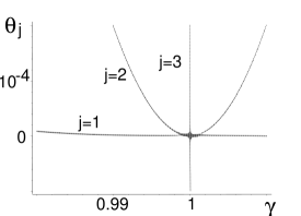
Figure 1: The decrease of the three lowest eigenvalues $\theta_{j}(\gamma)$ of the $N=4$ matrix (14) to zero for the growth of $\gamma$ to its maximal physical value $\gamma^{(EP)}=1$. The fourth root is much larger and lies out of the picture.

In the domain of small $\gamma$ and at $\delta=0$, the $\gamma-$proportionality coefficients (-3,-1,1,3) as given by Theorem 4 and its Corollary 5 get modified and replaced by the less compact set of quantities $-3/2\pm\sqrt{3}$ and $1/2\pm\sqrt{7}$, i.e., numerically, -3.23,-2.15, 0.23, 3.15, obtained as the roots of the leading-order secular polynomial $s^{4}+(2)\,s^{3}+(-21/2)\,s^{2}+(-39/2)\,s+81/16$.

6 Construction of metrics at $N\geq 5$

6.1 Physical Hilbert space at $N=5$

In the domain of very small $\gamma$ the process of the Hermitization of the CBH matrix Hamiltonians may be based on Theorem 4 at any $N$. Nevertheless, as long as the estimated $\gamma_{critical}\approx 1/(N-1)$ decreases quickly with the growth of $N$, the range of applicability of the linear approximation becomes more and more restricted. The higher-precision constructions become of an enhanced interest at $N\geq 5$.

6.1.1 General four-parametric metric

For

$$H^{(5)}_{(CBH)}(\gamma)=\left[\begin{array}[]{ccccc}-4\,i\gamma&2&0&0&0\\ \vskip 6.0pt plus 2.0pt minus 2.0pt\cr 2&-2\,i\gamma&\sqrt{6}&0&0\\ \vskip 6.0pt plus 2.0pt minus 2.0pt\cr 0&\sqrt{6}&0&\sqrt{6}&0\\ \vskip 6.0pt plus 2.0pt minus 2.0pt\cr 0&0&\sqrt{6}&2\,i\gamma&2\\ \vskip 6.0pt plus 2.0pt minus 2.0pt\cr 0&0&0&2&4\,i\gamma\end{array}\right]\,$$ (19)

we may consider the general Hermitian candidate for the metric with normalization $\Theta^{(5)}_{1,1}(\gamma)=1$,

$$\Theta^{(5)}(\gamma)=\left[\begin{array}[]{ccccc}{\it 1}&{\it{X}}+ix&{\it{Y}}+iy&{\it{Z}}+iz&{\it{W}}+iw\\ \vskip 6.0pt plus 2.0pt minus 2.0pt\cr{\it{X}}-ix&{\it{R}}&{\it{U}}+iu&{\it{V}}+iv&{\it{Z}}+iz\\ \vskip 6.0pt plus 2.0pt minus 2.0pt\cr{\it{Y}}-iy&{\it{U}}-iu&{\it{T}}&{\it{U}}+iu&{\it{Y}}+iy\\ \vskip 6.0pt plus 2.0pt minus 2.0pt\cr{\it{Z}}-iz&{\it{V}}-iv&{\it{U}}-iu&{\it{R}}&{\it{X}}+ix\\ \vskip 6.0pt plus 2.0pt minus 2.0pt\cr{\it{W}}-iw&{\it{Z}}-iz&{\it{Y}}-iy&{\it{X}}-ix&{\it 1}\end{array}\right]\,.$$ (20)

Its insertion in Eq. (4) yields the sequence of definitions of the four imaginary components of the first-row elements,

$$x=2\,{\it\gamma}\,,\ \ y=\sqrt{6}{\it\gamma}\,{\it{X}}\,,\ \ \ \ z=1/3\,{\it\gamma}\,\left(3\,{\it{Y}}+2\,{{\it\gamma}}^{2}\sqrt{6}\right)\sqrt{6}\,,\ \ \ \ w=v+{\it\gamma}\,{\it{Z}}-3\,{\it{X}}\,{\it\gamma}$$

as well as the two imaginary components of the second-row elements,

$$u=1/6\,{\it\gamma}\,\left(6+12\,{{\it\gamma}}^{2}+\sqrt{6}{\it{Y}}\right)\sqrt{6}\,,\ \ \ \ v=4\,{{\it\gamma}}^{3}{\it{X}}+3\,{\it{X}}\,{\it\gamma}+{\it\gamma}\,{\it{Z}}\,.$$

The real parts to be defined are the two off-diagonal items

$${\it{U}}=2\,{{\it\gamma}}^{2}\sqrt{6}{\it{X}}+1/2\,\sqrt{6}{\it{X}}+1/2\,\sqrt{6}{\it{Z}}\,,\ \ \ \ {\it{V}}={\it{W}}+{{\it\gamma}}^{2}\sqrt{6}{\it{Y}}+4\,{{\it\gamma}}^{4}+1/2\,\sqrt{6}{\it{Y}}$$

and their two diagonal partners

$${\it{R}}=1+1/2\,\sqrt{6}{\it{Y}}+6\,{{\it\gamma}}^{2}\,,\ \ \ \ {\it{T}}=1/6\,\left(4\,{\it{Y}}+8\,{{\it\gamma}}^{2}\sqrt{6}+8\,{{\it\gamma}}^{4}\sqrt{6}+8\,{{\it\gamma}}^{2}{\it{Y}}+\sqrt{6}+\sqrt{6}{\it{W}}\right)\sqrt{6}\,.$$

The resulting $\Theta^{(5)}(\gamma)=\Theta^{(5)}(\gamma,{X},{Y},{Z},{W})$ is a fairly compact candidate for the general four-parametric metric.

6.1.2 The requirement of positivity

The key technical obstacle arises when one wishes to specify the exact boundaries of the physical domain of the parameters for which the metric remains well defined, i.e., invertible and positive definite. For our present purposes we only need to know the metric at the small $\gamma$. In a way indicated by Corollary 5, the eigenvalues of the metric are then revealed positive and equidistant.

At $N=5$ the approximate metric candidate which is linear in $\gamma$ reads

$$\Theta^{(5)}_{0}(\gamma)=\left[\begin{array}[]{ccccc}1&2\,i{\it\gamma}&0&0&0\\ \vskip 6.0pt plus 2.0pt minus 2.0pt\cr-2\,i{\it\gamma}&1&i{\it\gamma}\,\sqrt{6}&0&0\\ \vskip 6.0pt plus 2.0pt minus 2.0pt\cr 0&-i{\it\gamma}\,\sqrt{6}&1&i{\it\gamma}\,\sqrt{6}&0\\ \vskip 6.0pt plus 2.0pt minus 2.0pt\cr 0&0&-i{\it\gamma}\,\sqrt{6}&1&2\,i{\it\gamma}\\ \vskip 6.0pt plus 2.0pt minus 2.0pt\cr 0&0&0&-2\,i{\it\gamma}&1\end{array}\right]\,.$$

The quintuplet of its exact eigenvalues $\theta_{j}=1+r_{j}$ coincides with the roots of the exact secular polynomial which gets completely factorized,

$$0=\left(\theta-1\right)\left(\theta-1+2\,{\it\gamma}\right)\left(\theta-1-2\,{\it\gamma}\right)\left(\theta-1-4\,{\it\gamma}\right)\left(\theta-1+4\,{\it\gamma}\right)\,.$$

For the proof it is sufficient to turn attention to the deviations $r_{j}$ from the unit value. Then, the exact  secular equation is again easily derived. As long as its explicit form becomes rather lengthy (containing as many as 22 terms), the detailed discussion of the mutual dependence of its parameters and roots would be a formidable task. Fortunately, once one omits all of the higher order corrections, the reduced equation reads ${r}^{5}-20\,{{\it\gamma}}^{2}{r}^{3}+64\,r{{\it\gamma}}^{4}=0$ and remains solvable easily yielding the roots $r$ proportional to $\gamma$ (i.e., small).

6.1.3 Two-parametric subfamily of metrics

In the models with $N=2$, 3 and 4 we saw that an important simplification resulted from the purely imaginary choice of $\Theta_{1,2}$. One of the consequences was the purely real form of $\Theta_{1,3}$. Let us now try to generalize this experience and introduce, tentatively, a chessboard-inspired ansatz with, in general, ${\rm Im\ }\Theta_{i,j}=0$ for $i+j=$ even and ${\rm Re\ }\Theta_{i,j}=0$ for $i+j=$ odd. At $N=5$ it reads

$$\Theta^{(5)}(y,w)=\left[\begin{array}[]{ccccc}1&ix&{\it y}&iz&{\it w}\\ \vskip 6.0pt plus 2.0pt minus 2.0pt\cr-ix&{\it{\rho}}&iu&{\it v}&iz\\ \vskip 6.0pt plus 2.0pt minus 2.0pt\cr{\it y}&-iu&{\it{\tau}}&iu&{\it y}\\ \vskip 6.0pt plus 2.0pt minus 2.0pt\cr-iz&{\it v}&-iu&{\it{\rho}}&ix\\ \vskip 6.0pt plus 2.0pt minus 2.0pt\cr{\it w}&-iz&{\it y}&-ix&1\end{array}\right]\,.$$

Here, in the light of Eq. (4) we have $x=2\,{\it\gamma}$, $z=\sqrt{6}{\it y}\,{\it\gamma}+4\,{{\it\gamma}}^{3}$, $u={\it y}\,{\it\gamma}+{\it\gamma}\,\sqrt{6}+2\,\sqrt{6}{{\it\gamma}}^{3}$ while $v=\sqrt{6}{\it y}\,{{\it\gamma}}^{2}+4\,{{\it\gamma}}^{4}+1/2\,{\it y}\,\sqrt{6}+{\it w}$. On the main diagonal we get ${\rho}=6\,{{\it\gamma}}^{2}+1+1/2\,{\it y}\,\sqrt{6}$ and ${\tau}=1+{\it w}+\left(4\,{\it y}+8\,{\it y}\,{{\it\gamma}}^{2}\right)/\sqrt{6}+8\,{{\it\gamma}}^{2}+8\,{{\it\gamma}}^{4}$. The resulting remarkable pattern of the distribution of the powers of $\gamma$ is best visible when we choose trivial $y=w=0$ and get the maximally elementary metric without free parameters,

$$\Theta^{(5)}=\left[\begin{array}[]{ccccc}1&2\,i{\it\gamma}&0&4\,i{{\it\gamma}}^{3}&0\\ \vskip 6.0pt plus 2.0pt minus 2.0pt\cr-2\,i{\it\gamma}&6\,{{\it\gamma}}^{2}+1&i{\it\gamma}\,\sqrt{6}\left(1+2\,{{\it\gamma}}^{2}\right)&4\,{{\it\gamma}}^{4}&4\,i{{\it\gamma}}^{3}\\ \vskip 6.0pt plus 2.0pt minus 2.0pt\cr 0&-i{\it\gamma}\,\sqrt{6}\left(1+2\,{{\it\gamma}}^{2}\right)&1+8\,{{\it\gamma}}^{2}+8\,{{\it\gamma}}^{4}&i{\it\gamma}\,\sqrt{6}\left(1+2\,{{\it\gamma}}^{2}\right)&0\\ \vskip 6.0pt plus 2.0pt minus 2.0pt\cr-4\,i{{\it\gamma}}^{3}&4\,{{\it\gamma}}^{4}&-i{\it\gamma}\,\sqrt{6}\left(1+2\,{{\it\gamma}}^{2}\right)&6\,{{\it\gamma}}^{2}+1&2\,i{\it\gamma}\\ \vskip 6.0pt plus 2.0pt minus 2.0pt\cr 0&-4\,i{{\it\gamma}}^{3}&0&-2\,i{\it\gamma}&1\end{array}\right]\,.$$ (21)

This matrix is positive definite (i.e., eligible metric) in the reasonably large interval of $\gamma\in(0,\gamma_{\max}^{(5)})$ where $\gamma_{\max}^{(5)}=1/2\,\sqrt{\sqrt{5}-1}\approx 0.5558929700$. The $\gamma-$dependence of the five eigenvalues $\theta_{j}$ is shown in Fig. 2.

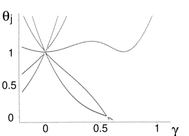
Figure 2: The $\gamma-$dependence of the eigenvalues of the $N=5$ matrix (21) and their positivity in the interval of $\gamma\in\left[0,\gamma_{\max}\right)$ with $\gamma_{\max}=1/2\,\sqrt{\sqrt{5}-1}$.

6.2 Physical Hilbert space at $N=6$

Our last explicit chessboard-inspired ansatz reads

$$\Theta^{(6)}=\left[\begin{array}[]{cccccc}1&{\rm i\,}x&{\it{y}}&{\rm i\,}z&{\it{w}}&{\rm i\,}{\mu}\\ \vskip 6.0pt plus 2.0pt minus 2.0pt\cr-{\rm i\,}x&{\it{\rho}}&{\rm i\,}u&{\it{v}}&{\rm i\,}{\it{\zeta}}&{\it{w}}\\ \vskip 6.0pt plus 2.0pt minus 2.0pt\cr{\it{y}}&-{\rm i\,}u&{\it{\tau}}&{\rm i\,}{\sigma}&{\it{v}}&{\rm i\,}z\\ \vskip 6.0pt plus 2.0pt minus 2.0pt\cr-{\rm i\,}z&{\it{v}}&-{\rm i\,}{\sigma}&{\it{\tau}}&{\rm i\,}u&{\it{y}}\\ \vskip 6.0pt plus 2.0pt minus 2.0pt\cr{\it{w}}&-{\rm i\,}{\it{\zeta}}&{\it{v}}&-{\rm i\,}u&{\it{\rho}}&{\rm i\,}x\\ \vskip 6.0pt plus 2.0pt minus 2.0pt\cr-{\rm i\,}{\mu}&{\it{w}}&-{\rm i\,}z&{\it{y}}&-{\rm i\,}x&1\end{array}\right].$$ (22)

Its imaginary matrix elements are all defined by formulae $x=\sqrt{5}{\it\gamma}$, $z=2\,\sqrt{5}{{\it\gamma}}^{3}\sqrt{2}+3\,{\it{y}}\,{\it\gamma}$ and ${\mu}=16\,{{\it\gamma}}^{5}+2\,{{\it\gamma}}^{3}\sqrt{2}\sqrt{5}{\it{y}}+\sqrt{5}{\it{w}}\,{\it\gamma}$ for the first row and by formulae $u=2\,{\it\gamma}\,\sqrt{2}-6/5\,\sqrt{5}{\it{y}}\,{\it\gamma}+3/5\,\left(2\,\sqrt{5}{{\it\gamma}}^{3}\sqrt{2}+3\,{\it{y}}\,{\it\gamma}\right)\sqrt{5}$, ${\zeta}=2/5\,\sqrt{2}\left(2\,\sqrt{5}{{\it\gamma}}^{3}\sqrt{2}+3\,{\it{y}}\,{\it\gamma}\right)\sqrt{5}+3/5\,\sqrt{5}{\it{w}}\,{\it\gamma}+16\,{{\it\gamma}}^{5}+2\,{{\it\gamma}}^{3}\sqrt{2}\sqrt{5}{\it{y}}$ and ${\sigma}=3\,{\it\gamma}-6/5\,\sqrt{2}\sqrt{5}{\it{y}}\,{\it\gamma}+3/5\,\sqrt{2}\left(2\,\sqrt{5}{{\it\gamma}}^{3}\sqrt{2}+3\,{\it{y}}\,{\it\gamma}\right)\sqrt{5}-2/5\,{{\it\gamma}}^{2}\sqrt{2}\left(2\,\sqrt{5}{{\it\gamma}}^{3}\sqrt{2}+3\,{\it{y}}\,{\it\gamma}\right)\sqrt{5}+1/5\,\sqrt{5}{\it{w}}\,{\it\gamma}+16\,{{\it\gamma}}^{5}+2\,{{\it\gamma}}^{3}\sqrt{2}\sqrt{5}{\it{y}}$ for the second and the third row. As long as $y$ and $w$ are kept as independent variables, we only have to define the remaining real matrix elements ${\rho}=8\,{{\it\gamma}}^{2}+1+2/5\,\sqrt{5}{\it{y}}\,\sqrt{2}$ and ${\tau}=3/5\,\sqrt{5}{\it{y}}\,\sqrt{2}+12\,{{\it\gamma}}^{2}-6/5\,\sqrt{2}\sqrt{5}{\it{y}}\,{{\it\gamma}}^{2}+6/5\,\sqrt{2}{\it\gamma}\,\left(2\,\sqrt{5}{{\it\gamma}}^{3}\sqrt{2}+3\,{\it{y}}\,{\it\gamma}\right)\sqrt{5}+1+3/5\,{\it{w}}\,\sqrt{5}$ on the main diagonal, and, last but not least, ${v}=4/5\,{\it\gamma}\,\left(2\,\sqrt{5}{{\it\gamma}}^{3}\sqrt{2}+3\,{\it{y}}\,{\it\gamma}\right)\sqrt{5}+3/5\,{\it{y}}\,\sqrt{5}+2/5\,\sqrt{5}{\it{w}}\,\sqrt{2}$.

These results confirm the expectations and extrapolation hypotheses. Once we accept the most natural simplification ${y}={w}=0$ and once we keep just the terms which are linear in $\gamma$ we get again the tridiagonal metric (18) with the factorized secular equation,

$$0=\left(\theta-1\right)\left(\theta-1+2\,{\it\gamma}\right)\left(\theta-1-2\,{\it\gamma}\right)\left(\theta-1-4\,{\it\gamma}\right)\left(\theta-1+4\,{\it\gamma}\right)\,.$$

After one incorporates the higher-order corrections we get the parameter-free version of the metric. The simplification of its matrix elements included $z=2\,\sqrt{5}{{\it\gamma}}^{3}\sqrt{2}$, $\mu=16\,{{\it\gamma}}^{5}$, $u=2\,{\it\gamma}\,\sqrt{2}+6\,{{\it\gamma}}^{3}\sqrt{2}$, ${\zeta}=8\,{{\it\gamma}}^{3}+16\,{{\it\gamma}}^{5}$ and $\sigma=3\,{\it\gamma}+12\,{{\it\gamma}}^{3}+8\,{{\it\gamma}}^{5}$ as well as ${\rho}=1+8\,{{\it\gamma}}^{2}$, ${\tau}=1+12\,{{\it\gamma}}^{2}+24\,{{\it\gamma}}^{4}$ and, finally, $v=8\,{{\it\gamma}}^{4}\sqrt{2}$. This enables us to display here the whole matrix, with its symmetry-determined matrix elements omitted,

$$\Theta^{(6)}_{(CBH)}=\left[\begin{array}[]{ccccc}1&i\sqrt{5}{\it\gamma}&0&\ldots&16\,i{{\it\gamma}}^{5}\\ \vskip 6.0pt plus 2.0pt minus 2.0pt\cr-i\sqrt{5}{\it\gamma}&1+8\,{{\it\gamma}}^{2}&2\,i\,\sqrt{2}\,{\it\gamma}\,\left(1+3\,{{\it\gamma}}^{2}\right)&\ldots&0\\ \vskip 6.0pt plus 2.0pt minus 2.0pt\cr 0&-2\,i\,\sqrt{2}\,{\it\gamma}\,\left(1+3\,{{\it\gamma}}^{2}\right)&1+12\,{{\it\gamma}}^{2}+24\,{{\it\gamma}}^{4}&\ldots&2\,i\sqrt{10}{{\it\gamma}}^{3}\\ \vskip 6.0pt plus 2.0pt minus 2.0pt\cr-2\,i\sqrt{10}{{\it\gamma}}^{3}&8\,\sqrt{2}\,{{\it\gamma}}^{4}&-i\,{\it\gamma}\,\left(3+12\,{{\it\gamma}}^{2}+8\,{{\it\gamma}}^{4}\right)&\ldots&0\\ \vskip 6.0pt plus 2.0pt minus 2.0pt\cr 0&-8\,i\,{{\it\gamma}}^{3}\left(1+2\,{{\it\gamma}}^{2}\right)&8\,{{\it\gamma}}^{4}\sqrt{2}&\ldots&i\sqrt{5}{\it\gamma}\\ \vskip 6.0pt plus 2.0pt minus 2.0pt\cr-16\,i{{\it\gamma}}^{5}&0&-2\,i\,\sqrt{10}\,{{\it\gamma}}^{3}&\ldots&1\end{array}\right]\,.$$ (23)

From the exact value of its smallest eigenvalue, incidentally, we managed to deduce the exact value of the domain-boundary quantity $\gamma^{(6)}_{\max}=1/2$. Moreover, we also managed to evaluate the second-order corrections to the eigenvalues of the metric $\theta_{j}=1+A_{j}\,\gamma+B_{j}\,\gamma^{2}+\ldots$. This result, summarized in Table 1, may be read as a strong encouragement of extrapolations towards $N>6$.

Table 1: Coefficients in the approximation $\theta^{(6)}_{j}(\gamma)=1+A_{j}\,\gamma+B_{j}\,\gamma^{2}+\ldots$

$j$	$A_{j}$	$B_{j}$
1	5	10
2	3	6
3	1	4
4	-1	4
5	-3	6
6	-5	10

Presumably, also many other features of the $N=6$ CBH model may be expected to find their analogues at the general matrix dimensions $N$. Among the clearest candidates, tendencies and patterns of possible extrapolations let us mention the last few hypotheses which could help us to reduce, in the future, the recurrences for the matrices $\Theta^{(N)}$ with polynomial entries to the recurrences for the mere arrays of the coefficients.

• At any $N$, the chessboard-inspired complex ansatz for $\Theta^{(N)}(\gamma)$ may be required to be a strictly real matrix after a formal analytic-continuation replacement of $\gamma$ by ${\rm i}\alpha$ with real $\alpha$;

• the powers $\gamma^{K_{n}}$ entering the matrix element $\Theta^{(N)}_{i,j}(\gamma)$ may be conjectured to be limited by the following empirical rules:

  1. $K_{n}$=even iff $i+j=$ even; $K_{n}$=odd iff $i+j=$ odd;

  2. $\min K_{n}=|i-j|$; $\max K_{n}=\min(|i+j-2|,|i+j-2N-2|)$.

7 Summary

Quantum theory offers a counterintuitive picture of reality. One has to replace, e.g., the energy of a classical system by an operator. In the most common unitary-evolution scenario such an operator (i.e., Hamiltonian) must be self-adjoint, $\mathfrak{h}=\mathfrak{h}^{\dagger}$. Once we admit a “hidden” interaction with environment, it may cause the loss of the self-adjointness of the “effective” Hamiltonian, $H\neq H^{\dagger}$ [23]. In parallel, the spectrum becomes complex and, due to the possible losses or gains from the environment, the evolution ceases to be unitary.

For a long time it escaped the attention of physicists that there also exists a fairly large family of quantum systems in which the Hamiltonians are admitted non-Hermitian but still, the system remains closed, exhibiting no interaction with an “environment”. The evolution is unitary, in an apparent contradiction with the Stone’s theorem. Fortunately, the paradox results from a misunderstanding: the “false” non-self-adjointness is detected in an ill-chosen Hilbert space ${\cal H}^{(F)}$.

Such an innovative use of non-Hermitian generators $H$ of the unitary evolution found its most persuasive success in nuclear physics [20] or in condensed-matter physics [41]. The more ambitious theoretical implementations of the idea were pursued in perturbation theory [42], in certain relativistic [43] and supersymmetric [44] extensions of quantum mechanics plus, perhaps, in quantum cosmology [45] and in quantum theory of catastrophes [46]. In all of these applications, Dieudonné relation (4) appeared to connect a given non-Hermitian observable Hamiltonian $H$ with all of its admissible Hermitizations, i.e., with all of the eligible physical Hilbert-space metrics $\Theta=\Theta(H)$. For our present Bose-Hubbard family (3) of quantum Hamiltonians, in particular, we were able to guarantee the stable, unitary evolution of the system via the construction of the operator $\Theta=\Theta(H)$ at small $\gamma$. For each representation (i.e., matrix dimension $N$) we recommended the direct solution of Dieudonné’s Eq. (4) and we showed that it is feasible.

For the first nontrivial matrix dimension $N=3$ we admit that the purely algebraic part of the task already looks rather complicated. Still, a suitable amendment of the approach made the construction feasible. The essence of the simplification lies in the ansatz for $\Theta(H)$ with symmetry with respect to the second diagonal. We revealed that such an assumption leads to the fully general three-parametric family of the candidates for the metric at $N=3$, and that it might open the way towards the study of models with general $N$.

At the higher $N\geq 4$ we encountered another obstacle during the determination of the boundary of the domain ${\cal D}$ of the “admissible” free parameters rendering the matrix of metric positive definite. This goal appeared overambitious and hopeless. It turned out that the construction could hardly be algebraic and/or non-numerical. Due to the enormous growth of the unfriendliness of secular polynomials the task of the proof of positivity of the candidates for the metric appeared next to impossible. Fortunately, in a climax of our paper we arrived at an innovative, feasible resolution of the problem. The proof has been found, thanks to the restriction of attention to the sufficiently small vicinity of the Hermitian limit $\Theta(H)\to I$, in the omission of the higher-powers of $\gamma$ and in the ultimate discovery of the elementary Lie-algebraic form of the leading-order difference $\Theta(H)-I\sim\gamma L_{y}+{\cal O}(\gamma^{2})$ and of the elementary factorizability of the secular polynomial.

References

- [1] H. Gersch and G. Knollman, Phys. Rev.. 129, 959 (1963); B. Wu and J. Liu, Phys. Rev. Lett. 96, 020405 (2006).
- [2] M. P. A. Fisher, P. B. Weichman, G. Grinstein and D. S. Fisher, Phys. Rev. B 40, 546 (1989).
- [3] L. Pitaevskii and S. Stringari, Bose-Einstein Condensation (Clarendon, Oxford, 2003); T. Giamarchi, Ch. Rüegg and O. Tchernyshyov, Nature Physics. 4, 198 (2008); V. Zapf, M. Jaime and C.-D. Batista, Rev. Mod. Phys. 86, 563 (2014); Erratum Rev. Mod. Phys. 86, 1453 (2014); M. Kreibich, J. Main, H. Cartarius and G. Wunner, Phys. Rev. A 93, 023624 (2016); L. Schwarz, H. Cartarius, Z. H. Musslimani, J. Main and G. Wunner, Phys. Rev. A 95, 053613 (2017).
- [4] O. Dutta, M. Gajda, P. Hauke, M. Lewenstein, D.-S. Lühmann, B. A. Malomed, T. Sowinski and J. Zakrzewski, Rep. Prog. Phys. 78, 066001 (2015).
- [5] J. M. Zhang and R. X. Dong, Eur. J. Phys. 31, 591 (2010).
- [6] E. M. Graefe, U. Günther, H. J. Korsch and A. E. Niederle, J. Phys. A: Math. Theor 41, 255206 (2008).
- [7] M. Hiller, T. Kottos and A. Ossipov, Phys. Rev. A 73, 063625 (2006); L. Jin and Z. Song, Ann. Phys. (NY) 330, 142 (2013).
- [8] C. M. Bender, Rep. Prog. Phys. 70, 947 (2007).
- [9] A. Mostafazadeh, Int. J. Geom. Meth. Mod. Phys. 7, 1191 (2010).
- [10] F. Bagarello, J.-P. Gazeau, F. H. Szafraniec and M. Znojil, Eds., Non-Selfadjoint Operators in Quantum Physics: Mathematical Aspects (Wiley, Hoboken, 2015).
- [11] T. Kato, Perturbation Theory for Linear Operators (Springer-Verlag, Berlin, 1966).
- [12] M. V. Berry, Czech. J. Phys. 54, 1039 (2004); S. Klaiman, U. Günther and N. Moiseyev, Phys. Rev. Lett. 101, 080402 (2008); W. D. Heiss, J. Phys. A: Math. Theor. 45, 444016 (2012); A. Fring, J. Phys. A: Math. Theor. 48, 145301 (2015); B. Peng, S. K. Ozdemir, M. Liertzer, W.-J. Chen, J. Kramer, H. Yilmaz, J. Wiersig, S. Rotter and L. Yang, Proc. NAS USA 113, 6845 (2016); K. Ding, G.-C. Ma, M. Xiao, Z.-Q. Zhang and C.-T. Chan, Phys. Rev. X 6, 021007 (2016); M. Grundmann, C. Sturm, C. Kranert et al, Phys. Status Solidi - Rapid Res. Lett. 11, 1600295 (2017).
- [13] M. Znojil, Phys. Rev. A, to appear (arXiv: 1808.07472).
- [14] F. Bagarello, Phys. Rev. A 88, 032120 (2013); M. Znojil, Ann. Phys. (NY) 336, 98 (2013); D. I. Borisov, Acta Polytech. 54, 93 (2014); E. Caliceti and S. Graffi, in [10], p. 189; D. I. Borisov, F. Růžička and M. Znojil, Int. J. Theor. Phys. 54, 4293 (2015).
- [15] D. I. Borisov and M. Znojil, in “Non-Hermitian Hamiltonians in Quantum Physics”, F. Bagarello, R. Passante and C. Trapani, eds. (Springer, Berlin, 2016), p. 201.
- [16] M. Znojil, Phys. Rev. A 97, 042117 (2018).
- [17] F. M. Fernández and J. Garcia, Ann. Phys. (NY) 342, 195 (2014); L. Jin and Z. Song, Phys. Rev. A 93, 062110 (2016); J. Garcia and R. Rossignoli, Phys. Rev. A 96, 062130 (2017).
- [18] Y. N. Joglekar and A. K. Harter, Photon. Res. 6, A51 (2018).
- [19] R. León-Montriel et al, arXiv:1805.08393.
- [20] F. G. Scholtz, H. B. Geyer and F. J. W. Hahne, Ann. Phys. (NY) 213, 74 (1992).
- [21] M. Znojil, Phys. Rev. D 78, 085003 (2008); B. Gardas, S. Deffner and A. Saxena, Phys. Rev. A 94, 022121 (2016).
- [22] J. Dieudonne, in Proc. Int. Symp. on Lin. Spaces (Pergamon, Oxford, 1961), p. 115.
- [23] N. Moiseyev, Non-Hermitian Quantum Mechanics (CUP, Cambridge, 2011); S. Garmon, M. Gianfreda and N. Hatano, Phys. Rev. A 92, 022125 (2015); I. Rotter and J. P. Bird, Rep. Prog. Phys. 78, 114001 (2015).
- [24] S. Sachdev, Quantum Phase Transitions (CUP, Cambridge, 2011).
- [25] B. C. Hall, Quantum Theory for Mathematicians (Springer, New York, 2013).
- [26] H. J. Lipkin, N. Meshkov and A. J. Glick, Nucl. Phys. 62, 188 (1965); P. Stránský, M. Dvořák, and P. Cejnar, Phys. Rev. E 97, 012112 (2018).
- [27] C. M. Bender and K. A. Milton, Phys. Rev. D 55, 3255 (1997).
- [28] C. M. Bender and S. Boettcher, Phys. Rev. Lett. 80, 5243 (1998).
- [29] M. Znojil, Symm. Integr. Geom. Methods Appl. (SIGMA) 5, 001 (2009) (e-print overlay: arXiv:0901.0700).
- [30] M. Znojil, I. Semorádová, F. Růžička, H. Moulla and I. Leghrib, Phys. Rev. A 95, 042122 (2017).
- [31] H. F. Jones, Phys. Rev. D 78, 065032 (2008).
- [32] A. Messiah, Quantum Mechanics I (North-Holland, Amsterdam, 1961).
- [33] D. Krejčiřík, V. Lotoreichik, and M. Znojil, Proc. Roy. Soc. A 20180264, in print (arXiv:1804.06766).
- [34] M. Znojil, Phys. Lett. A 379, 2013 (2015); M. Znojil, Ann. Phys. (NY) 385, 162 (2017).
- [35] T. J. Milburn, J. Doppler, C. A. Holmes et al, Phys. Rev. A 92, 052124 (2015); J. Doppler, A. A. Mailybaev, J. Böhm, et al, Nature 537, 76 (2016).
- [36] M. Znojil, Symm. Integr. Geom. Methods Appl. (SIGMA) 4, 001 (2008) (arXiv overlay: 0710.4432v3).
- [37] Y. Ma and A. Edelman, Linear Algebr. Appl. 273, 45 (1998); M. Znojil, Phys. Rev. A 97, 032114 (2018).
- [38] M. H. Stone, Ann. Math. 33, 643 (1932).
- [39] M. Znojil, J. Phys. A: Math. Theor. 41, 244027 (2008).
- [40] M. Znojil, J. Phys. A: Math. Theor. 45, 085302 (2012).
- [41] F. J. Dyson, Phys. Rev. 102, 1217 (1956).
- [42] V. Buslaev and V. Grechi, J. Phys. A: Math. Gen. 26, 5541 (1993).
- [43] A. Mostafazadeh, Ann. Phys. (New York) 309, 1 (2004).
- [44] A. A. Andrianov, M. V. Ioffe, F. Cannata et al., Int. J. Mod. Phys. A 14, 2675 (1999); M. Znojil, F. Cannata, B. Bagchi et al., Phys. Lett. B 483, 284 (2000); P. Dorey, C. Dunning and R. Tateo, J. Phys. A: Math. Gen. 34, L391 (2001); M. Znojil and V. Jakubský, Pramana - J. Phys. 73, 397 (2009); B. Bagchi, A. Banerjee and A. Ganguly, J. Math. Phys. 54, 022101 (2013).
- [45] A. A. Andrianov, Ch. Lan and O. O. Novikov, in “Non-Hermitian Hamiltonians in Quantum Physics”, F. Bagarello, R. Passante and C. Trapani, eds. (Springer, Berlin, 2016), p. 29; M. Znojil, in “Non-Hermitian Hamiltonians in Quantum Physics”, F. Bagarello, R. Passante and C. Trapani, eds. (Springer, Berlin, 2016), p. 383.
- [46] M. Znojil, J. Phys. A: Math. Theor. 45, 444036 (2012); G. Lévai, F. Růžička and M. Znojil, Int. J. Theor. Phys. 53, 2875 (2014); M. Znojil, Symmetry 8, 52 (2016); S. Longhi, Optics Lett. 43, 2929 (2018).