A Model for
Auto-Programming for General Purposes

Abstract: The Universal Turing Machine (TM) is a model for VonNeumann computers — general-purpose computers. A human brain can inside-skull-automatically learn a universal TM so that he acts as a general-purpose computer and writes a computer program for any practical purposes. It is unknown whether a machine can accomplish the same. This theoretical work shows how the Developmental Network (DN) can accomplish this. Unlike a traditional TM, the TM learned by DN is a super TM — Grounded, Emergent, Natural, Incremental, Skulled, Attentive, Motivated, and Abstractive (GENISAMA). A DN is free of any central controller (e.g., Master Map, convolution, or error back-propagation). Its learning from a teacher TM is one transition observation at a time, immediate, and error-free until all its neurons have been initialized by early observed teacher transitions. From that point on, the DN is no longer error-free but is always optimal at every time instance in the sense of maximal likelihood, conditioned on its limited computational resources and the learning experience. This letter also extends the Church-Turing thesis to automatic programming for general purposes and sketchily proved it.

Keywords: Auto-programming, AI, machine learning, Turing machines, universal Turing machines, neural networks, GENISAMA, vision, audition, natural language understanding

It remains elusive how a biological brain represents, computes, learns, memorizes, updates, and abstracts through its life-long experience—from a zygote, to embryo, fetus, newborn, infancy, childhood, and adulthood. Gradually, the brain produces behaviors that are increasingly rule-like [1, 2, 3] and can perform auto-programming for general purposes. By auto-programming, we mean that a brain automatically generates a sequence of procedures, from tying shoelaces, to making a business plan, to writing a computer program. Such programs are not just random shufflers. They must relate to meanings of the world — namely physics gives rise to meanings [4, 5].

Here, we greatly simplify such rich processes of co-development of brain and body through activities, assisted by innate (i.e., prenatally developed) reflexes and innate motivations [6, 7], to realize auto-programming from facts, education, engineering, thinking, fiction, and discovery. We ask only: What is a minimal set of mechanisms that enables a biological or silicon machine to learn auto-programming for general purposes? Some early examples from an answer below are in a companion paper.

Three conceptual steps guide us toward this answer. We first extend Finite Automata (FAs) [8, 9] to agents in the sense that states are not hidden but are open as actions. Then we extend such agent FAs to attentive agent FAs, so that the machines can automatically attend only a subset of current inputs (e.g., some words among all words on this page). Finally we introduce the GENISAMA TM by replacing all symbols in such attentive agent FAs with patterns that naturally emerge from the real world.

Agent FA: Two variants of FA, Moore machines and Mealy machines [8, 9] output actions but not their states. We extend an FA to agent [10], called Agent FA, by simply requiring it to output its current state entirely, but its current actions are included in the current state. This extension is conceptually important because the current state is now teachable as actions so that we are ready to address the issue of internal representations in neural networks below. In psychology, all skills and knowledge fall into two categories [11], declarative (e.g., verbal) and non-declarative (e.g., bike riding). Therefore, all skills and knowledge can be expressed as actions.

Attentive Agent FA: Suppose that a symbolic street scene at time $t$ has multiple objects. E.g.,

$$S(t)=\{\mbox{car1, car2, sign1, sign2, pedestrian1, ...}\}$$

Instead of taking only one input symbol $\sigma$ at a time (e.g., $\sigma=\mbox{car1}$), an attentive agent FA attends to a set of symbols at a time (e.g., $s(t)=\{\mbox{car1, pedestrian1\}}\subset S(t)$). The control of any TM is an Attentive Agent FA as we will discuss below.

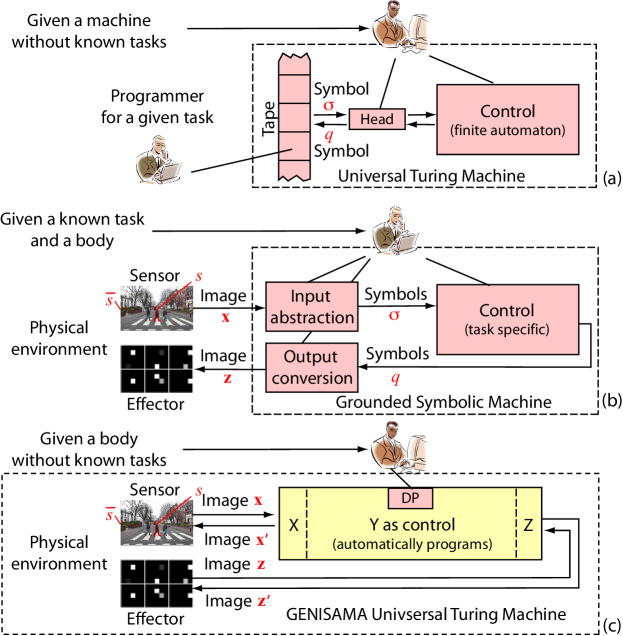
Figure 1: Three categories of agents, (a) Universal Turing Machines that is symbolic and cannot auto-program, (b) Grounded Symbolic Machines that are task-specific and cannot auto-program, and (c) GENISAMA Universal Turing Machines whose Developmental Program are task-nonspecific. A GENISAMA Universal Turing Machines can auto-program for general purposes. The tape in (a) becomes the real world and all the symbols in (a) and (b) become natural patterns. DP: Developmental Program. $X$: the sensory port. $Z$: the effector port. $Y$: the hidden “bridge for “banks” $X$ and $Z$. Pink block: human handcrafted. Yellow blocks: emerge automatically.

In order to understand auto-programming for general purposes, we need to first discuss the Universal TM [12, 8, 9].

Recently, it has been proved [13] that the control of any TM is an FA as illustrated in Fig. 1(a). Using this new result, our examples in Methods are much simpler.

Theorem 1

The control of a TM is not only an Agent FA, but also an Attentive Agent FA.

The proof is in Methods.

A Universal TM is for general purposes [8, 9]. The input tape of a Universal TM has two parts, the program as instructions and the data for the program to use, not just data like a regular TM. Theorem 1 is also true for any Universal TM because it is a special kind of TM.

Because the input is a set of symbols instead of a symbol, the transition table of an Attentive Agent FA, especially as the control of a Universal TM, is typically extremely large — impractical to handcraft.

Next, we drop symbols altogether for our machine. Why? A symbol is atomic, whose meanings are in the programmer’s document, not told to the symbolic TM. They are also too static for real-time tasks. Suppose you, assisted by a symbolic TM, drive into a new country that uses a new language (e.g., new signs) but the programmer of your symbolic TM has not considered this new language. Your biological brain immediately deals with the patterns (e.g., images) of new signs directly without the programmer’s document because you can pull your car over and start to learn. Namely, your brain starts to auto-reprogram itself. But your symbolic TM in Fig. 2(b) cannot because all its symbols are static and your programmer has left you! Weng [14] proved that your brain is free of symbols for a complexity reason.

For auto-programming, we need a new theory that uses exclusively natural patterns (e.g., image patches of cars and signs). The six necessary conditions are in the acronym GENISAMA below.

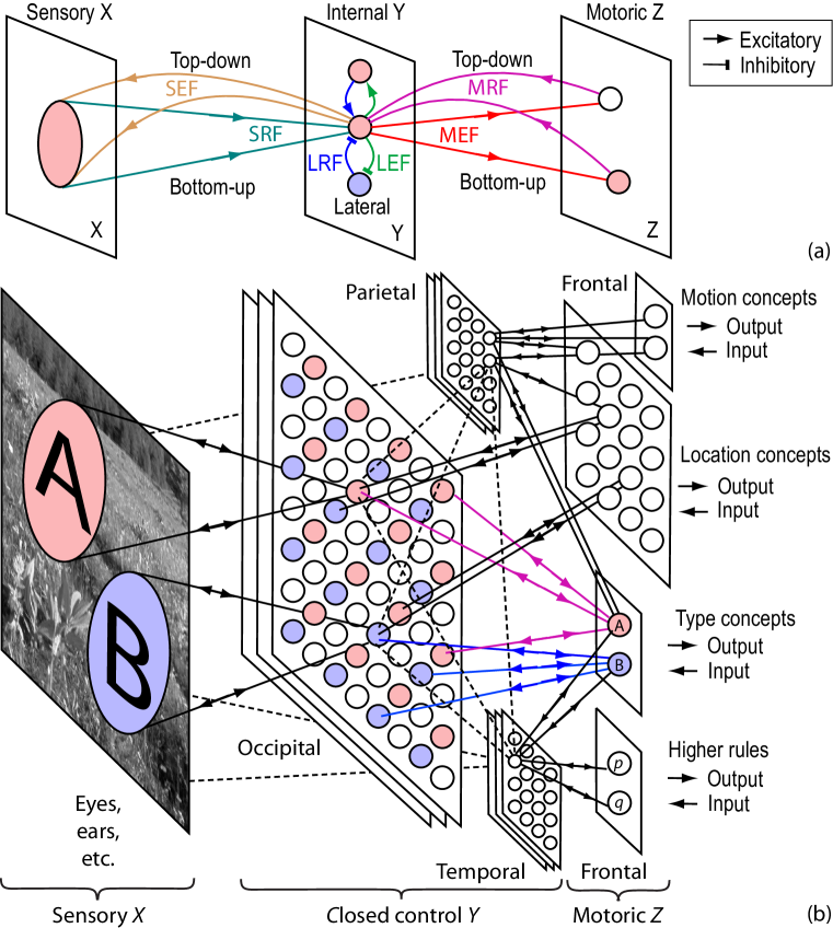
Figure 2: Brain $Y$ is theoretically modeled as the two-way bridge of the sensory bank $X$ and the motor bank $Z$. The bridge, mathematically denoted by Eq. (3), is extremely rich: Self-wiring within a Developmental Network (DN) as the control of GENISAMA TM, based on statistics of activities through “lifetime”, without any central controller, Master Map, handcrafted features, and convolution. (a) Each feature neuron has six fields in general. S: Sensory; M: motoric; L: lateral; R: receptive; E: effective; F: field. But simulated neurons in $X$ do not have Sensory Receptive Field (SRF) and Sensory Effective Field (SEF) because they only effect $Y$ and those in $Z$ do not have Motor Receptive Field (MRF) and Motoric Effective Field (MEF) because they only receive from $Y$. (b) The resulting self-wired architecture of DN with Occipital, Temporal, Parietal, and Frontal lobes. Regulated by a general-purpose Developmental Program (DP), the DN self-wires by “living” in the physical world. The $X$ and $Z$ areas are supervised by physics, including self, teachers, and other physical events. Through the synaptic maintenance [15, 16], some $Y$ neurons gradually lost their early connections (dashed lines) with $X$ ($Z$) areas and become “later” (early) $Y$ areas. In the (later) Parietal and Temporal lobes, some neurons further gradually lost their connections with the (early) Occipital area and become rule-like neurons. These self-wired connections give rise to a complex dynamic network, with shallow and deep connections instead of a deep cascade of areas. Object location and motion are non-declarative concepts and object type and language sequence are declarative concepts [11]. Concepts and rules are abstract with the desired specificities and invariances. See Methods for why DN do not have any static Brodmann areas.

GENISAMA TM: As illustrated in Fig. 1(c) it has a Developmental Network (DN) as its control and the real (physical) world as its “tape”. The DN has three areas, sensory $X$, hidden $Y$ and motoric $Z$ with details shown in Fig. 2. We also use $X$, $Y$, $Z$ to denote the spaces, respectively, of the corresponding neuronal response patterns.

If $X$ and $Z$ contain all sensors and effectors of an agent, $Y$ models the entire hidden “brain”. If $X$ and $Z$ correspond to a subpart of the brain areas, $Y$ models the brain area that connect $X$ and $Z$ as a two-way “bridge”. The computational meanings of the acronym GENISAMA are as follows:

Grounded: All patterns $\mathbf{z}\in Z$ and $\mathbf{x}\in X$ are from the external environment (i.e., the body and the extra-body world), not from any symbolic tape.

Emergent: All patterns $\mathbf{z}\in Z$ and $\mathbf{x}\in X$ emerge from activities (e.g., images). All vectors $\mathbf{y}\in Y$ emerge automatically from $\mathbf{z}\in Z$ and $\mathbf{x}\in X$.

Natural: All patterns $\mathbf{z}\in Z$ and $\mathbf{x}\in X$ are natural from real sensors and real effectors, without using any task-specific encoding, as illustrated in Fig. 2.

Incremental: The machine incrementally updates at times $t=1,2,...$. Namely DN uses $(\mathbf{z}(t),\mathbf{x}(t))$ for update the network and discard it before taking the next $(\mathbf{z}({t+1}),\mathbf{x}({t+1}))$. We avoid storing images for offline batch training (e.g., as in ImageNet) because the next image $\mathbf{x}({t+1})$ is unavailable without first generating and executing the agent action $\mathbf{z}(t)$ which typically alters the scene that determines $\mathbf{x}({t+1})$.

Skulled: As the skull closes the brain to the environment, everything inside the $Y$ area (neurons and connections) are initialized at $t=0$ and off limit to environment’s direct manipulation after $t=0$.

Attentive: In every cluttered sensory image $\mathbf{x}\in X$ only the attended parts correspond to the current attended symbol set $s$. In every cluttered motoric image $\mathbf{z}\in Z$ only the attended parts correspond to the current state symbol $q$ (e.g., firing muscle neurons in the mouth and arms). Two symbols correspond to a pattern (not necessarily connected, as in $s=\{\mbox{car2, pedestrian1\}}$).

Motivated: Different neural transmitters have different effects to different neurons, e.g., resulting in (a) avoiding pains, seeking pleasures and speeding up learning of important events and (b) uncertainty- and novelty-based neuronal connections (synaptic maintenance for auto-wiring) and behaviors (e.g., curiosity).

Abstractive: Each learned concept (e.g., object type) in $Z$ are abstracted from concrete examples in $\mathbf{z}\in Z$ and $\mathbf{x}\in X$, invariant to other concepts learned in $Z$ (e.g., location, scale, and orientation). E.g., the type concept “dog” is invariant to “location” on the retina (dogs are dogs regardless where they are). Invariance is different from correlation: dog-type and dog-location are correlated (e.g., dogs are typically on ground).

The GENISAMA control as DN: Assume a human knowledge base is representable by a grand TM, whose FA control has alphabet $\Sigma=\{\sigma_{1},\sigma_{2},...,\sigma_{n}\}$, a set of states $Q=\{q_{1},q_{2},...,q_{m}\}$, and a static lookup table as its transition function $\delta:Q\times\Sigma\mapsto Q$. The lookup table has $n$ columns for $n$ input symbols and $m$ rows for $m$ states. Each transition of the FA control is from state $q_{i}$ and input $\sigma_{j}$, to the next state $q_{k}$, denoted as $(q_{i},\sigma_{j})\rightarrow q_{k}$, corresponding to the $q_{k}$ entry stored at row $i$ and column $j$, in the lookup table.

Required by GENISAMA, let grounded $n$ (emergent) vectors $X=\{\mathbf{x}_{1},\mathbf{x}_{2},...,\mathbf{x}_{n}\}$ represent the $n$ (static) symbols in $\Sigma$, so that $\mathbf{x}_{j}\equiv\sigma_{j},j=1,2,...,n$ where $\equiv$ means “corresponds to”. Likewise, let $m$ (emergent) vectors $Z=\{\mathbf{z}_{1},\mathbf{z}_{2},...,\mathbf{z}_{m}\}$ represent the $m$ (static) symbols in $Q$, so that $\mathbf{z}_{i}\equiv q_{i},i=1,2,...,m$. Thus, each symbolic transition (left, static) in FA corresponds to the vector mapping (right, emergent) in DN:

$$[(q_{i},\sigma_{j})\rightarrow q_{k}]\equiv[(\mathbf{z}_{i},\mathbf{x}_{j})\rightarrow\mathbf{z}_{k}].$$

Because of the reasons in Weng [14], the lookup table for the human common-sense base is exponentially wide and exponentially high, but also extremely sparse. Yet, the right-side in the above equation uses only observed sparse entries emerged, where each entry corresponds to a neuron in DN.

Denote $\dot{\mathbf{v}}=\mathbf{v}/\|\mathbf{v}\|$, i.e., normalizing the Euclidean length of $\mathbf{v}$.

The neurons in $X$ and $Z$ are open to the environment, supervisable by the environment.

Next, let the Grand TM in the environment teach the DN by supervising its $X$ and $Z$ ports while TM runs, one transition at a time in real time. The DN has its brain area $Y$ area hidden (i.e., skulled).

The simplest DN learns incrementally as follows. Given each observation $(\mathbf{z},\mathbf{x})$ from the teacher TM, all $Y$ neurons compute their goodness of match. Each $Y$ neuron $(i,j)$ corresponds to an observed transition at the $(i,j)$ entry of the lookup table. In order to match both $\mathbf{z}$ and $\mathbf{x}$, it has a two-part weights $\mathbf{v}_{ij}=(\mathbf{t}_{ij},\mathbf{b}_{ij})$. When the best match is not perfect explained below, $(\mathbf{z},\mathbf{x})$ is the left-side of a new transition; so DN incrementally adds one more $Y$ neuron by setting its $\mathbf{t}_{ij}=\mathbf{z}_{i}$ and $\mathbf{b}_{ij}=\mathbf{x}_{j}$. So, DN adds up to (finite) $mn$ hidden neurons, but typically much fewer because the lookup table is sparse.

The top-down match value is $v_{t}=\dot{\mathbf{t}}\cdot\dot{\mathbf{z}}$; and bottom-up match $v_{b}=\dot{\mathbf{b}}\cdot\dot{\mathbf{x}}$. We know that $\dot{\mathbf{a}}\cdot\dot{\mathbf{b}}=\cos\theta$, where $\theta$ is the angle between the two unit vectors $\dot{\mathbf{a}}$ and $\dot{\mathbf{b}}$. $\cos\theta=1$ is maximized if and only iff $\dot{\mathbf{a}}=\dot{\mathbf{b}}$, namely $\theta=0$. The match between the current context input $(\mathbf{z},\mathbf{x})$ with the weight $(\mathbf{t},\mathbf{b})$ of a $Y$ neuron is the sum (or product) of the bottom-up and top-down match values, as its pre-response value:

$$f(\mathbf{z},\mathbf{x}\;|\;\mathbf{t},\mathbf{b})=v_{t}+v_{b}=\dot{\mathbf{t}}\cdot\dot{\mathbf{z}}+\dot{\mathbf{b}}\cdot\dot{\mathbf{x}}$$

Only the best matched $Y$ neuron fires (with response value 1), determined by a highly nonlinear competition:

$$(i^{\prime},j^{\prime})=\arg\max_{(i,j)\in Y}f(\mathbf{z},\mathbf{x}\;|\;\mathbf{t}_{ij},\mathbf{b}_{ij})=\arg\max_{(i,j)\in Y}\{\dot{\mathbf{t}}_{ij}\cdot\dot{\mathbf{z}}+\dot{\mathbf{b}}_{ij}\cdot\dot{\mathbf{x}}\}.$$

All other loser $Y$ neurons do not fire (response value 0), because otherwise these neurons not only create more noise but also lose their own long-term memory (since all firing neurons must update using input).

The area $Z$ incrementally updates so that the firing $Y$ neuron $(i^{\prime},j^{\prime})$ is linked to all firing components (i.e., 1 not 0) in $\mathbf{z}_{k}$, so DN accomplishes every observed transition $(\mathbf{z}_{i},\mathbf{x}_{j})\rightarrow\mathbf{z}_{k}$, error-free, as proved in Weng [13].

Using the optimal Hebbian learning in Methods, Weng [13] further proved that (1) the weight vector of each $Y$ neuron in the optimal (maximum likelihood) estimate of observed samples in $(X,Z)$, (2) the weight from each $Y$ neuron $(i^{\prime},j^{\prime})$ to each $Z$ neuron $k$ is the probability for $(i^{\prime},j^{\prime})$ to fire, conditioned on $k$ fired, and (3) overall, the response vectors $\mathbf{y}$ and $\mathbf{z}$ are both optimal (maximum likelihood).

Thus, DN uses at most $mn$ $Y$ neurons, observes each symbolic transition $(q_{i},\sigma_{j})\rightarrow q_{k}$ in TM represented by vector transition $(\mathbf{z}_{i},\mathbf{x}_{j})\rightarrow\mathbf{z}_{k}$, and learns each error-free if each input $(\mathbf{z},\mathbf{x})$ is noise-free. If input $(\mathbf{z},\mathbf{x})$ is noisy, DN is optimal. Namely, DN both “overfits” and is optimal, regardless input is noisy or noise-free. This is a new proof for TM emerging from DN, shorter but less formal than Weng [13].

Attention corresponds to weights $\mathbf{t}$ and $\mathbf{b}$ partially connected with $Z$ area and $X$ area, respectively, — thanks to naturally emerging patterns $\mathbf{z}$ and $\mathbf{x}$.

Auto-programming: Consider two learning modes. Mode 1: Learn from a teacher TM supervised. Mode 2: Learn from the real physical world without any explicit teacher. For early learning in Mode 1 to be useful for further learning in Mode 2, assume that the patterns in Mode 1 are grounded in (i.e., consistent with) the physical world of Mode 2.

Theorem 2

By learning from any teacher TM (regular or universal) through patterns (Modes 1 and 2) with top-1 firing in $Y$, the DN control enables a learner GENISAMA TM to emerge inside it with the following properties.

1. Sufficient neurons situation: The GENISAMA TM is error-free for all learned TM transitions (Mode 1) and resubstitution of all observed physical experiences (Mode 2).

2. Insufficient neurons situation: This happens when the finite $n$ $Y$ neurons have all been activated. The action at time $t+1$ is optimal in the sense of maximum likelihood (but not error-free) in representing the observed context space $(\mathbf{z},\mathbf{x})$, conditioned on the amount of computational resource $n$ and the experience of learning for all discrete times $0,1,2,...,t$.

The proof sketch is available in Methods.

Next, consider auto-programming for general purposes. We represent each purpose as a TM. Suppose a Grand Transition Table $G$ represents the FA control of a grand TM. This $G$ contains a Universal TM $T_{u}$ and a finite number of tasks as TMs, $T_{i}$, $i=1,2,...$. Traditionally, $T_{u}$ is based on a (symbolic) computer language, but here $T_{u}$ can be in a (non-symbolic) natural language if it is GENISAMA.

Theorem 3

A GENISAMA TM inside DN automatically programs for general purposes $T_{i},i=1,2,...$, after it has learned a Universal TM $T_{u}$ and the related purposes $T_{i},i=1,2,...$. However, the DN algorithm (developmental program) itself is task-independent and language-independent (e.g., English or Chinese).

The proof sketch is available in Methods.

The Church-Turing thesis is a hypothesis that (A) a function on natural numbers is computable by a human using a pencil-and-paper method if and only if (B) it is computable by a TM. This hypothesis is considered not provable because (A) involves a human who senses and acts in the real world whose process was not sufficiently formulated before to make a proof possible. The GENISAMA TM sufficiently formulates human auto-programming in the real-world and therefore a full proof now becomes possible. The following theorem extends the Church-Turing thesis.

Theorem 4

For any machine, natural or artificial, the following (a), (b) and (c) are equivalent in terms of computing engine: (a) Its GENISAMA augmentation learns and does auto-programing for general purposes in the real world. (b) It computes all functions that are computable using a pencil-and-paper method. (c) It computes all functions computable by TMs.

The proof sketch is in Methods. Therefore, it has been constructively proved (sketchy) in theory that a machine can perform auto-programming for general purposes. These constructive proofs explain also how to. The companion paper shows how to practically approach strong AI.

Methods

Before we discuss the detail of the new methods, let us first review major methods in the literature.

In Artificial Intelligence, there are two schools, symbolic and connectionist [17, 14, 18]. On one hand, the meanings of symbolic representations (e.g., Bayesian Nets [19, 20], Markov models [21, 22], graphic models by many) are static (before probability measures) in the human designer’s mind and design documents, but are not told to the machine. For example, such symbolic representations prevent the machine from learning the meanings of new concepts beyond those having already been statically handcrafted. On the other hand, representations in artificial neural networks can emerge from activities but lack [17, 18] clearly understandable logic, such as abstraction, invariance, and the hierarchy of relationships. For example, deep learning networks [23, 24, 25, 26, 27, 28] and other brain inspired network models [29, 30] have shown impressive capabilities. However, they lack a crucial function that appears to be necessary to scale up from a human fetus, to human infant, to human adulthood: a system automatically and directly learns from physical world for open domains.

The work there demonstrate, through a constructive (sketchy) proof, that this requires a framework that is beyond from-pixels-to-handcrafted-text [23, 24, 29, 30, 25, 26, 27, 28], that is not an emergent-and-symbolic-hybrid [29, 27, 28, 31] either, but rather whose representations are exclusively emergent and there are no symbols in DN at all. In such a drastically different architecture and its representations, detection, recognizing, attention, and action on individual object(s) all take place in parallel in cluttered environments where background pixels are often many more than object pixels.

Unique in this regard, representations in DN [32], supported by a series of embodiments called Where-What Networks, WWN-1 through WWN-9, take the best of both AI schools: not only emergent, but also logic; not only logic, but also complete in the sense of TM [13]. However, it is unknown whether a DN can auto-program for general purposes. The work here takes up this fundamental issue: Can machines automatically learn to think for general purposes — not relying on any handcrafted symbols, let alone any world models?

In Natural Intelligence, the task-nonspecificity of an innate Developmental Program (DP) is highly debatable [33, 34, 35, 36, 37, 38, 39]. It is still unclear computationally how a DP can regulates a neural network, natural or artificial, to enable the network to auto-program concepts and rules from the cluttered physical environment. This paper proposes a computational theory for that without claiming to be biologically complete. Since spontaneous neuronal activities are present prenatally [40, 41], the activity-dependent wiring mechanisms here could take place both before and after birth. The model proposed here contains supports for both nativism and empiricism, but more explicit and precise computationally.

Theories of machine-learning logical computations have been fruitfully studied (e.g., [42, 43, 44]) to deal with propositions and predicates, whose answers are, yes or no (e.g., fraud or not fraud), but not both. The full automation of machine learning in the real world — e.g., the emergence of representations (i.e., skull closed, through lifetime learning of an open series of unpredictable tasks) and automatic scaffolding (i.e., early-learned simple skills automatically assist later learning of more complex skills) — has not received sufficient attention. However, this is the way for brains to autonomously learn from infancy to adulthood. Since the Autonomous Mental Development (AMD) direction was proposed in [39], a major progress in this direction, represented by the Where-What Networks [32] as embodiments of DN, has not received sufficient attention either (see, e.g., recent reviews [26, 25, 44]). However, the full automation of machine learning seems to be a practical way for machines to become as versatile as a 3-year-old human child in the three well acknowledged bottleneck areas of AI — vision, audition and natural language understanding. The theory here is necessary for the full automation of machine learning.

Through Finite Automata [8, 9], we extend such logic to spatiotemporal sensorimotor actions, to deal with kinds of intelligence that require behaviors, including vision, audition (recognition of not only speech, but also music, etc.), natural language acquisition, and vision-guided navigation. Namely, not only logic, but also interactive actions where logic is a special case. This letter focuses on theory and algorithm; a companion paper submitted concurrently focuses on experiments. We will see that auto-programming is necessary for the full automation of machine learning and also explains how a human adult can do so.

There are two types of approaches to modeling a brain. The first type assumes that the genome rigidly dictates all Brodmann areas (e.g., V1 and V2) inside the brain so such a model starts with static existence of the Brodmann areas such as those reported by [45]. The second type, which this model belongs to, does not assume so. Such a model does not have static brain areas because the formation of, and the existence of, brain areas depend on activities, as demonstrated by the following studies:

1. Cells in the V1 area selectively respond to the left eye, the right eye, and both eyes in a normal kitten; but they respond only to one eye if the other eye is closed from birth [46]. Namely, where an area connects from is plastic.

2. A pathway amputation early in life enabled the auditory cortex to receive visual signals through actively growing neurons so that the auditory cortex emerged visual representations and the animal demonstrated visual capabilities using rewired auditory cortex [47]. Namely, what an area does is plastic.

3. The visual cortex is reassigned to audition and touch in the born blind [48]. Namely, visual areas may completely disappear.

Therefore, the DP of this model does not specify Brodmann areas. It enables “general purpose” neurons to wire, trim, and re-wire. But the experimental demonstration for the formation of the spinal cord and the detailed Brodmann areas in the DN, as well as the plasticity thereof, remains to be future work.

The following questions are: Is there a central controller in the brain? Is there a Master Map in the brain? Does the genome rigidly specify features or instead features emerge from both prenatal (i.e., innate) and postnatal development? Does the brain uses convolution — replication of neural weights across different neurons? Does the brain consist of a rigid deep cascade of processing modules? Inspired by the above plasticity studies, the new theory here does not assume the static existence of a Master Map proposed by Anne Treisman 1980 [49, 50] and used by others [51, 52, 53, 54]. Such a Master Map requires a central controller who is already intelligent, so that it selects every attended object image-patch from each figure-ground-mixed image on the retina and feeds only attended figure patch into the Master Map. In the Master Map, the location and scale of the figure are normalized so that remaining issue is only classification. In some sense, the “normalization” that we hope is performed by the motoric area $Z$ in the theory area, but $Z$ is not a feature map but an action map.

In the Computational Vision literature, such a central controller is a human. Bottom-up features [55, 56] and their saliencies have been proposed [52, 54, 57] to partially serve the role of this central controller — a salient patch is fed into the Master Map. Another example of human central controller is Cresceptron [58, 24] and much later work where the human trainer manually draws a polygon on the sensed image that segments a human attended figure from the ground so that the system learns bottom-up from only pixels inside the polygon. However, the brain anatomy [45, 59] appears to allude to us that the brain network contains various shallow and deep circuits in which bi-directional connections are almost everywhere, not just a cascade. The new theory here assumes that neurons automatically connect, not only bottom-up, but also top-down [60, 61, 62, 63, 64, 65] and lateral, all using accumulated statistics in neuronal activities.

Deep learning convolutional networks [66] with max-pooling [24, 67] and other techniques [68, 69, 70, 26, 27, 25, 44] have shown their power in pattern classification — output class labels. They all imposed a cascade of processing modules/layers. The max-pooling is meant to reduce the location resolution from each early layer to the next layer to avoid the exponential explosion of the template size of convolution. However, the amount of computation can be contained by enabling each $Y$ feature neuron — in early and later layers — to have two input sources, bottom-up from $X$ and top-down from $Z$. Therefore, not only location “resolution” is automatically reduced from early to later $Y$ areas through the ventral pathway (for outputting class information), but also the type “resolution” is also automatically reduced from early to later $Y$ areas through the dorsal pathway (for outputting location- and manipulation-information). This top-down and bottom-up two-input $(\mathbf{z},\mathbf{x})$ architecture seems to provide a more flexible architecture for dealing with pattern recognition, either from monolithic or from cluttered scenes. Such a non-cascade network seems to be consistent with neuroanatomical studies reviewed in [45].

Agent FA To understand how a symbolic state can abstract both spatial and temporal contexts, consider Task 1: Produce the truth-value of an input logic-AND expression like:

$$T\wedge F\wedge T\wedge T$$

written on a tape. A regular FA only has an input string not a tape but this tape-view is useful next. We allow the tape head to read the input sequence by moving only right, a symbol at a time, and to read only. In general, such a logic-AND expression consists of a finite number of input symbols from alphabet $\Sigma=\{T,F,\wedge\}$, where $T$ and $F$ represent true and false, respectively, and $\wedge$ denotes logic AND. Let $Q$ be the set of states of the FA handcrafted by a human programmer.

The control of an Agent FA is a function $\delta:Q\times\Sigma\mapsto Q$, a mapping from domain $Q\times\Sigma$ to codomain $Q$.

Table I gives the control for Task 1, where the meaning of each state is denoted by the subscript of $q$. The patterns for $\mathbf{x}$ and $\mathbf{z}$ will be needed later in the paper. At row $q$ and column $\sigma$ is the next state $q^{\prime}=\delta(q,\sigma)$, or denoted graphically as $(q,\sigma)\rightarrow q^{\prime}$. E.g., at the initial state $q_{0}$, receiving an input $T$, the next state is $q_{T}$ to memorize the context $T$. This gives $\delta(q_{0},T)=q_{T}$. Similarly, $\delta(q_{T},\wedge)=q_{T\wedge}$ to memorize context $T\wedge$. Then, $q^{\prime}=\delta(q_{T\wedge},F)=q_{F}$, because $T\wedge F=F$. The transition sequence for the above input $T\wedge F\wedge T\wedge T$ is

$$q_{0}\stackrel{{\scriptstyle T}}{{\longrightarrow}}q_{T}\stackrel{{\scriptstyle\wedge}}{{\longrightarrow}}q_{T\wedge}\stackrel{{\scriptstyle F}}{{\longrightarrow}}q_{F}\stackrel{{\scriptstyle\wedge}}{{\longrightarrow}}q_{F\wedge}\stackrel{{\scriptstyle T}}{{\longrightarrow}}q_{F}\stackrel{{\scriptstyle\wedge}}{{\longrightarrow}}q_{F\wedge}\stackrel{{\scriptstyle T}}{{\longrightarrow}}q_{F}.$$ (1)

The state $q_{-}$ represents that the input sequence is an invalid logic-AND expression, e.g., $\wedge TF$ or $F\wedge\wedge$.

TABLE I: Control $\delta$ of FA for Task 1 and the pattern representations of state $q$ and input $\sigma$.

$\delta(q,\sigma)$		Input $\sigma$	$T$	$F$	$\wedge$
State $q$	State pattern $\mathbf{z}$	Input pattern $\mathbf{x}$	010	011	100
$q_{0}$	001		$q_{T}$	$q_{F}$	$q_{-}$
$q_{T}$	010		$q_{-}$	$q_{-}$	$q_{T\wedge}$
$q_{F}$	011		$q_{-}$	$q_{-}$	$q_{F\wedge}$
$q_{T\wedge}$	100		$q_{T}$	$q_{F}$	$q_{-}$
$q_{F\wedge}$	101		$q_{F}$	$q_{F}$	$q_{-}$
$q_{-}$	110		$q_{-}$	$q_{-}$	$q_{-}$

This is temporal abstraction from examples: Each state memorizes only the necessary context information for the specific Task 1. The abstraction in the previous state facilitates the abstraction of the next state. In natural language acquisition, the temporal context for each state is similar but more complex.

As spatial abstraction from examples, we can extend the Task 1 so as to handle symbol $\tau$ as $T$ and $\phi$ as $F$, respectively. All we need to do is expand Table I by adding two additional columns for inputs $\tau$ and $\phi$, respectively, but using the same next states as $T$ and $F$. During vision-guided autonomous driving, different traffic semaphores are like $T$ and $\tau$ here, but more complicated.

Thus, both spatial and temporal abstractions take place concurrently in each transition: $(q,\sigma)\rightarrow q^{\prime}$. We will see in Table IV below that when a brain applies this mechanism to patterns, the brain deals with space and time in a unified way, independent of meanings.

It is useful below to see how the control implements Table I: Given any state $q$ and input $\sigma$, the control finds the matched row $q$ at row and matched column $\sigma$. The table cell stores the information for the next state $q^{\prime}$. Below, each table cell will correspond to a neuron whose inputs are the original patterns (not symbols) of $q$ and $\sigma$ as shown in Table I.

In Task 1, inputs $T$ and $T\wedge T$ lead to the same state $q_{T}$. This process requires state design and equivalent-state finding for spatiotemporal abstraction. Handcrafted by humans, such symbolic representations are logic and clean [17, 18]. But they become manually intractable and thus error-prone (brittle) when the transition table has exponentially many rows and columns for natural languages or autonomous driving [71, 72, 14, 73, 74]. Below, we will see that the natural world can supervise each transition $(q,\sigma)\rightarrow q^{\prime}$ but using directly patterns which are without human handcrafting.

Attentive Agent FA An Attentive Agent FA has a set of input symbols, called alphabet $\Sigma$, of a finite size. At each time $t$, $t=1,2,...$, it attends to a set $\Sigma(t)\subset\Sigma$ of symbols from the symbolic environment $E(t)$ [75, 76, 77, 78, 79, 80, 64]. The set $\Sigma(t)$ can be a 2-D patch of text (e.g., of this page) or a substring of the input sequence (e.g., $T\wedge F$ of $T\wedge T\wedge F\wedge T$). The state/action from the machine may change the environment and also the next sensed $\Sigma(t+1)$.

In Task 1, the single-letter-right-only scan is only one of many ways of the Attentive Agent FA. For an unconstrained Attentive Agent FA, a human programmer must handcraft a large lookup table $\delta:Q\times 2^{\Sigma}\mapsto Q$ so that the output state $q(t)\in Q$ at every time $t$ enables the Attentive Agent FA to sequentially complete the given task. The number of columns of the transition table of $\delta$ is exponential in the size of $\Sigma$ because of the power set $2^{\Sigma}$ in the domain of $\delta$. The number of rows, the size of $Q$, may potentially also be exponential in the size of $\Sigma$.

Task 1 does not need this freedom of attention. However, an Attentive Agent FA is useful for the more challenging Task 2: Produce the truth value of an input sequence that includes logic operators $\wedge$, $\vee$, and parentheses, such as:

$$T\wedge((T\vee F)\wedge T\vee F).$$

It is known [8, 9] that the single-letter-right-only scan can still accomplish Task 2 if the machine has an infinite-size stack so that it can store an unbounded number of left parentheses.

If the machine can write onto the tape, the machine is a TM illustrated in Fig. 1(a) without the need for the stack. A human can program a TM to perform Task 2 [8, 9].

Proof of Theorem 1: The control of a TM has a transition function $\delta:Q\times\Gamma\mapsto Q\times\Gamma\times D$, where $Q$, $\Gamma$ and $D=\{R,L,S\}$ are the sets of states, the tape alphabet, and head moves, respectively. We extend $\delta$ to $\delta^{\prime}:Q^{\prime}\times\Gamma\mapsto Q^{\prime}$ which is the form of the control of an Agent FA, where $Q^{\prime}=Q\times\Gamma\times D$. We have proved that the control of a TM is an Agent FA. The above extension of domain from $Q\times\Gamma$ of $\delta$ to $Q^{\prime}\times\Gamma$ of $\delta^{\prime}$ means that for all $q^{\prime}=(q,\gamma,d)\in Q\times\Gamma\times D$ and $\gamma^{\prime}\in\Gamma$, $\delta^{\prime}(q^{\prime},\gamma^{\prime})=\delta(q,\gamma^{\prime})$. Namely $\delta^{\prime}$ is independent of, or does not attend to, the last written symbol $\gamma$ and head move $d$ in its domain (as they are often encoded in state). But this attention is dynamic, as the head can scan multiple positions to reach a state. Namely, the control is an Attentive Agent FA. This ends the proof.

A Grounded Symbolic Machine illustrated in Fig. 1(b) can deal with additionally input patterns (image, lidar, sound, etc.), but it cannot automatically program for general purposes because it still requires a human programmer to handcraft the meanings of every input symbol $\sigma$ used to represent its input features, internal states $q$, and output actions. A probability version [81] alleviates the uncertainty in such symbols, but cannot address the inadequacy of static symbols to represent a new town, or a new situation (e.g., rain or hacker laser [82] for lidar)

Neural networks (e.g., [83, 84] and many others) have been using patterns directly; but traditional neural networks do not have grounded symbol-like capabilities [4, 17, 11]. Bridging this gap requires a machine to learn not only symbol-like concepts directly from non-symbols but also attention rules — to quickly capture relevant patches (e.g., $s$ in Fig 1(b)) that are necessary for immediate action and disregard remainders (e.g., $\bar{s}$ in Fig 1(b)). Such attention rules are implicit; we often attend without knowing reasons. The intractability of handcrafting such implicit rules demands general-purpose auto-programming.

GENISAMA TM. Early neural network models for FA [85, 86, 87] and for TM [88, 89] are laudable for computing the automata mapping using networks but they used special encodings and do not learn, having none of GENISAMA. E.g., the TM in [88, 89] used 2-D registered inputs (one signal line and the other line means the presence of signal in the signal line). In contrast, the inputs in $X$ here are unregistered (e.g., an object can appear anywhere in the image) and cluttered (typically more noise/background dimensions than signal dimensions). The TM in [89] extends to irrational numbers using infinitely long numbers, but words of a finite length should be sufficient for a practical GENISAMA TM (e.g., it recognizes and understand the irrational number $\sqrt{2}$ by the shape $\sqrt{2}$ and its rules instead of the infinitely long number).

The environment of the control DN is divided into internal environment (e.g., the network that learns an equivalent lookup table for the control but more efficient than exponential) and external environment. The external environment includes the body of the agent and extra-body environment.

Each area of DN control may have multiple subareas: $X$ may contain two retinae, two cochlear hair cell arrays, somatosensory arrays, and receptor arrays of other sensory modalities. $Z$ may contain muscle arrays for the mouth, the arms, and effectors of other motor modalities. $Y$ as the internal representation of the control senses the pattern in its input space $Z\times X=\{(\mathbf{z},\mathbf{x})\;|\;\mathbf{z}\in Z,\mathbf{x}\in X\}$ to produce $Y$ patterns. In turn, each of $X$ and $Z$ uses the $Y$ pattern to further predict the pattern in themselves. Motivated by brain plasticity discussed below, we let subareas in $Y$ to automatically emerge (like Brodmann areas [59, 90]) instead of statically handcrafted.

Suppose, in Table II, a GENISAMA TM learns from a teacher TM. The teacher is via its Attentive Agent FA control and the learner is via its DN control. For clarity, suppose that each area of DN finishes an update computation in a unit time. Then, let every area of DN run in discrete times $t=0,1,2,...$ in parallel. The Attentive Agent FA does not have any internal area because it is symbolic—a lookup table is sufficient. The DN takes an additional unit time for the $Y$ area to update and interpolate. That is why Table II only needs to specify the Attentive Agent FA at even time instants.

TABLE II: The correspondence between the symbolic Attentive Agent FA and the DN control of GENISAMA TM

$\left[\begin{array}[]{c}q(0)\\ \sigma(0)\end{array}\right]$	$\rightarrow$	$\rightarrow$	$\rightarrow$	$\left[\begin{array}[]{cc}\emptyset&\overline{q(2)}\\ \emptyset&\underline{\sigma(2)}\end{array}\right]$	$\rightarrow$	$\rightarrow$	$\rightarrow$	$\left[\begin{array}[]{cc}\emptyset&\overline{q(4)}\\ \emptyset&\underline{\sigma(4)}\end{array}\right]$	$\rightarrow$	$\cdots$
$\left[\begin{array}[]{c}\mathbf{z}(0)\\ \mathbf{x}(0)\end{array}\right]$	$\rightarrow$	$\mathbf{y}(1)$	$\rightarrow$	$\left[\begin{array}[]{cc}\emptyset&\overline{\mathbf{z}^{\prime}(2)}\\ \emptyset&\underline{\mathbf{x}^{\prime}(2)}\end{array}\right]$	$\rightarrow$	$\mathbf{y}(3)$	$\rightarrow$	$\left[\begin{array}[]{cc}\emptyset&\overline{\mathbf{z}^{\prime}(4)}\\ \emptyset&\underline{\mathbf{x}^{\prime}(4)}\end{array}\right]$	$\rightarrow$	$\cdots$
$\mathbf{y}(0)$	$\rightarrow$	$\left[\begin{array}[]{cc}\emptyset&\overline{\mathbf{z}^{\prime}(1)}\\ \emptyset&\underline{\mathbf{x}^{\prime}(1)}\end{array}\right]$	$\rightarrow$	$\mathbf{y}(2)$	$\rightarrow$	$\left[\begin{array}[]{cc}\emptyset&\overline{\mathbf{z}^{\prime}(3)}\\ \emptyset&\underline{\mathbf{x}^{\prime}(3)}\end{array}\right]$	$\rightarrow$	$\mathbf{y}(4)$	$\rightarrow$	$\cdots$

In Table II, the first row is the time flow of the Attentive Agent FA control of the teacher TM where $q(t)$ and $\sigma(t)$, $t=0,2,4,...$, are the attended state/action and input, respectively.

A traditional FA does not predict input at all (see Eq. (1)), but we require an FA or Attentive Agent FA to predict not only the next state $q^{\prime}$ but also the next input $\sigma^{\prime}$. New here is that we use $q$ and $\sigma$ both to predict also $\sigma^{\prime}$:

$$\left[\begin{array}[]{c}q\\ \sigma\end{array}\right]\rightarrow\left[\begin{array}[]{c}q^{\prime}\\ \sigma^{\prime}\end{array}\right].$$ (2)

The more obstructively complete $q$ is, the better the prediction for $\sigma^{\prime}$. When such a prediction of $\sigma^{\prime}$ is not unique, the agent is immature to explain the attended environment. A calf might be mature in terms of finding food, but immature in terms of avoiding its predators.

With the real time indices in Table II, the framework of Bayesian Networks [19, 10] can be applied to the Attentive Agent FA while avoid cyclic graphs in graphical models because each cycle occurs at a different time instance above. This deals with the problem of cyclic graphs that static graphic models have avoided.

In each $2\times 2$ array inside Table II, the first column is predicted by the control and the second has been affected by supervision from the environment. $\emptyset$ means an empty set—the prediction is undetermined. An underline for input (e.g., $\underline{\sigma(2)}$) or overline for state/action (e.g., $\overline{q(2)}$) means the environment supervises and the supervision is different from what the control predicted.

The control DN of GENISAMA TM learns from the teacher TM by taking one taught $(q^{\prime},\sigma^{\prime})$ at a time in Eq. (2), but dealing with patterns directly. Symbolically, it learns a mapping $\delta:Q\times\Sigma\mapsto Q\times\Sigma$ from the teacher TM (e.g., mother or school instructor).

The DN uses original patterns $\mathbf{z}(t)$ and $\mathbf{x}(t)$ whose attended parts correspond to symbols $q(t)$ and $\sigma(t)$, respectively, denoted as $a(\mathbf{z}(t))\equiv q(t)$ and $a(\mathbf{x}(t))\equiv\sigma(t)$ where function $a$ is a dynamically learned function that marks off the unattended components.

Running at times $t=0,1,2,3,4,...$, the 2nd and 3rd rows in Table II are two flows that run in parallel to predict the corresponding patterns $\mathbf{x},\mathbf{y},\mathbf{z}$ in all the three areas of the DN. The $Y$ area takes input from $(\mathbf{z},\mathbf{x})$ to produce a response vector $\mathbf{y}$ which is then used by $Z$ and $X$ areas to predict $\mathbf{z}$ and $\mathbf{x}$ respectively:

$$\left[\begin{array}[]{c}\mathbf{z}\\ \mathbf{x}\end{array}\right]\rightarrow\mathbf{y}\rightarrow\left[\begin{array}[]{c}\mathbf{z}^{\prime}\\ \mathbf{x}^{\prime}\end{array}\right]$$ (3)

where the first $\rightarrow$ denotes the update in the left side using the left side as input. Like the FA, each prediction in Eq. (3) is called a transition. The same principle is also used to predict the binary (or real-valued) $\mathbf{x}^{\prime}\in X$ in Eq. (3). The quality of prediction depends on how state/action $\mathbf{z}$ abstracts the external world sensed by $\mathbf{x}^{\prime}$.

Learning As the simplest version, we use a highly recurrent, winner-take-all computation to simulate parallel lateral inhibition in $Y$: the $Y$ area with $n$ neurons responds with $\mathbf{y}=(y_{1},y_{2},...y_{n})$ where

$$y_{j}=\begin{cases}1&\mbox{if $j=\underset{1\leq i\leq n}{\operatorname{argmax}}\{f_{i}(\mathbf{z},\mathbf{x})\}$}\\ 0&\mbox{otherwise}\end{cases}$$ (4)

$j=1,2,...n$, where each $f_{i}$ measures the goodness of match between its input patch in $(\mathbf{z},\mathbf{x})$ and its weight vector $(\mathbf{z}_{i},\mathbf{x}_{i})$. The Hebbian learning together with the synaptic maintenance explained below initialize, update, cut-and-grow, all weight vectors $(\mathbf{z}_{i},\mathbf{x}_{i})$, $i=1,2,...,n$, resulting the rich connections illustrated in Fig. 2.

Let the FA control of the teacher TM have $r$ rows and $c$ columns. Suppose that in the learner GENISAMA TM, the $Y$ area has at least $n=rc$ $Y$ neurons. For Table I, $n=rc=6\times 3=18$. Without any central controller, all $Y$ neurons start with random weights at time $t=0$. At each time $t$, $t=1,2,...$, only the winner $Y$ neuron fires at response value 1 and incrementally updates its weight vector $(\mathbf{z}_{i},\mathbf{x}_{i})$ as the vector average of attended part of $(\mathbf{z},\mathbf{x})$. Then, the $i$-th $Y$ neuron memorizes perfectly the $i$-th distinct input pair $(\mathbf{z},\mathbf{x})$ observed in life.

The learner GENISAMA TM is taught by the teacher TM through the supervision of $(\mathbf{z},\mathbf{x})$. Each $Z$ neuron represents a unique component in $\mathbf{z}$. It should fire at 1 (instead of not firing at 0) if and only if it has been taught to fire right after the firing $Y$ neuron. This is true regardless in how many $Z$ patterns this $Z$ neuron appears. In general, if the number of $Y$ neurons is insufficient and input in $(\mathbf{z},\mathbf{x})$ has noise, the weight from the firing $Y$ neuron to each $Z$ neuron is the incrementally updated probability for the pre-synaptic $Y$ neuron to fire conditioned on that the post-synaptic $Z$ neuron fires.

Therefore, the roles of working memory and long-term memory in each area $Y$ are dynamic — the firing neurons are the current working memory and all other currently non-firing neurons are the current long-term memory. In this way, it is always the best matched neurons to update while other non-firing neurons keep their memory intact. When the number of $Y$ neurons is large, the finite-size DN appears to never run out of memory because the top-matched neurons are near and the forgetting/update is for the nearest memory only.

Top-k and brain areas In general, top-$k$ $(k>1)$ neurons fire, as members of a distributed $Y$ “committee” in which only $k$ experts fire to vote, as illustrated in Fig. 2(b). The top-$k$ mechanism itself is not biologically plausible, but it simulates mutual inhibitions among neurons (see Fig. 2(a)) so that much fewer $Y$ neurons fire in the presence of mutual inhibitions (see sparse coding idea [91]).

The top-$k$ voting in Eq. (3) was called the “bridged-islands” model [92]. In general, the “bridge” $Y$ area can be considered any brain area where neurons fire to be used by its connected islands — top islands $Z$ and bottom islands $X$. The complex brain network hierarchy (e.g., see [45]) is not a cascade as modeled in deep learning. Each area is a bridge that provides feature detectors for all neurons that are statistically correlated through excitatory connections and anti-correlated through inhibitory connections (see [93]). Consequently, the sensory end of DN is the most concrete, having 100% sensory content and 0% motoric content. The motor end of DN is the most abstract, 0% sensory and 100% motoric. Other areas in DN are in-between, developing intermediate abstract features that correspond to intermediate invariances (see, e.g., Figs. 6.5 and 6.6 in [93]). This avoids the forced feedback loop in electrical engineering — from the most abstract $Z$ back to the most concrete $X$ (see, e.g., [27]).

Dynamic learning modes The open ports $Z$ and $X$ are supervised or free, depending on the external and internal environments. By “supervised”, we mean that, as soon as the port predicts a pattern as the left-column in each $2\times 2$ array in Table II, the external world overrides it as the right column of the $2\times 2$ array. Otherwise, the $Z$ port is “free”, predicting/generating actions from within. If the “eye” is closed, the $X$ port is not supervised by the external environment and the $X$ port predicts “mental images”. (But “mental images” can, in principle, emerge also from early subareas in $Y$ like LGN, V1 etc. or written on a piece of paper through actions in $Z$, not requiring the eyes to close.)

Never directly supervised, the closed $Y$ uses unsupervised learning—optimal Hebbian learning explained below, although the agent’s action maybe supervised by a teacher through the $Z$ area. Namely, the body of the agent always supervises DN, but the $Y$ area always uses unsupervised learning!

Let us look at the example in Eq. (1). We must let $q$ and $\sigma$ predict in parallel:

$$\left[\begin{array}[]{c}q_{0}\\ \underline{T}\end{array}\right] \rightarrow \left[\begin{array}[]{cc}\emptyset&\overline{q_{T}}\\ \emptyset&\underline{\wedge}\end{array}\right]\rightarrow\left[\begin{array}[]{cc}\emptyset&\overline{q_{T\wedge}}\\ \emptyset&\underline{F}\end{array}\right]\rightarrow\left[\begin{array}[]{cc}\emptyset&\overline{q_{F}}\\ \emptyset&\underline{\wedge}\end{array}\right]\rightarrow\left[\begin{array}[]{cc}\emptyset&\overline{q_{F\wedge}}\\ \emptyset&\underline{T}\end{array}\right]$$ (15)

$$\rightarrow \left[\begin{array}[]{cc}\emptyset&\overline{q_{F}}\\ \emptyset&\underline{\wedge}\end{array}\right]\rightarrow\left[\begin{array}[]{cc}q_{F\wedge}&q_{F\wedge}\\ T&T\end{array}\right]\rightarrow\left[\begin{array}[]{c}q_{F}\\ \wedge\end{array}\right].$$ (22)

where the last two predictions are perfect because of two reasons: (a) the two predictions of state are unique due to the teacher consistency; (b) the two predictions of input are unique since the learner is still naive — only $T$ follows $(q_{F},\wedge)$ and it has not seen illegal input. (Without better states that model the physical causality of input sequence, such symbolic prediction of input is not guaranteed to be unique.)

Using the patterns in Table I, which are meaningless here but should correspond to naturally emerging images, the DN learns the above teacher sequence one transition at a time, but through original patterns only and via $Y$ neurons:

$$\left[\begin{array}[]{c}001\\ \underline{010}\end{array}\right] \rightarrow y_{1}\rightarrow \left[\begin{array}[]{cc}\emptyset&\overline{010}\\ \emptyset&\underline{100}\end{array}\right]\rightarrow y_{2}\rightarrow\left[\begin{array}[]{cc}\emptyset&\overline{100}\\ \emptyset&\underline{011}\end{array}\right]\rightarrow y_{3}\rightarrow\left[\begin{array}[]{cc}\emptyset&\overline{011}\\ \emptyset&\underline{100}\end{array}\right]\rightarrow y_{4}\rightarrow\left[\begin{array}[]{cc}\emptyset&\overline{101}\\ \emptyset&\underline{010}\end{array}\right]$$ (33)

$$\rightarrow y_{5}\rightarrow \left[\begin{array}[]{cc}\emptyset&\overline{011}\\ \emptyset&\underline{100}\end{array}\right]\rightarrow y_{4}\rightarrow\left[\begin{array}[]{cc}101&101\\ 010&010\end{array}\right]\rightarrow y_{5}\rightarrow\left[\begin{array}[]{c}011\\ {100}\end{array}\right]$$ (40)

where $y_{i}$, $i=1,2,...,5$, corresponds to the first five initialized $Y$ neurons. Two $Y$ neurons $y_{4}$ and $y_{5}$ predict perfectly when the same (or similar) pattern of $(q,\sigma)$ appears again. The term “similar” means interpolation that is impossible in Eq. (22).

Attention For simplicity, we have assumed above that $\mathbf{z}$ and $\mathbf{x}$ do not contain unattended parts. Of course, in general the prediction of $\mathbf{x}$ pattern can cover fewer than all sensory bits (3 bits above), amounting to experienced-based global-or-local sensory attention — predicted bits are attended. Namely, how the learner machine attended in the past “lifetime” shapes how it likely attends in the future “lifetime”.

This example shows the model’s separation of DP mechanisms (i.e., table lookup) from the meanings of the learned task. Namely, the human programmer of the DP does not need to know the meanings of patterns in Eq. (40) that emerge. A regular TM and a Universal TM differ in the meanings of input symbols and state symbols, but they use the same domain $Q^{\prime}\times\Sigma$ and codomain $Q^{\prime}$ (i.e., table lookup) for their control function $\delta^{\prime}$. Therefore, the table lookup mechanism for Eq. (40) is sufficient for not only a regular TM but also a Grand TM that contains many TMs and some Universal TMs.

Scaffolding Scaffolding means simple skills learned early assist the learning of complex skills later [94, 95]. Imagine that while the automaton grows from “embryo” to “adult”, such meanings become increasingly sophisticated and are internalized as clusters in the later $Y$ areas (see Fig. 2). These state/action patterns may also be of any complex meanings, e.g., “goals” and “intents” [65] that are taught/learned in the “language” of actions. In rats goals have been found in the pre-frontal cortex [96]. Such meanings may entail creativities, as self-generated programs through predictions like those in Eq. (40). Off-task processes [97] (i.e., the automaton takes a short break from task execution to “think”) allow generalizations/creativities, through the seemingly-rigid pattern prediction in Eq. (40).

Computational complexity Assume that the dimension (e.g., number of pixels) of $X$ is $\alpha$. Each component of $X$ has $10$ possible (e.g., color) values. Then, there are $c=10^{\alpha}$ possible $X$ patterns.

Let the $Z$ area has $\beta$ concept zones (4 in Fig. 2), where each zone has $10$ concept values. There are $r=10^{\beta}$ possible $Z$ patterns.

Then, there are $rc=10^{\alpha}10^{\beta}=10^{\alpha+\beta}$ possible patterns in $(\mathbf{z},\mathbf{x})$, exponential in $\alpha$ and $\beta$. For example, when $\alpha=640\times 480$ (pixels) and $\beta=4$ (zones), the transition table for FA already requires $10^{1228800}$ entries, $10^{1228789}$ times more than the number of neurons in a human brain! Note, the table is sparse as many entries are not observed but could appear in “life”.

In contrast, the control DN uses a large (e.g., $n=10^{11}$ for a human brain) but constant number $n$ of $Y$ neurons to interpolate among observed patterns for dealing with exponentially many $rc=10^{\alpha+\beta}$ patterns. It may use $n\beta$ bottom-up weights of $Z$ to interpolate among observed $Y$ patterns for exponentially many possible $Z$ patterns. Similarly, it uses $n\alpha$ top-down weights of $X$ to interpolate among observed $Y$ patterns for exponentially many possible $X$ patterns.

Namely, the update for each DN takes a (large) constant amount of time, so DN has a linear time complexity $O(nt)$ in $t$ while running in real time $t$ and $n$ is a large constant.

The GENISAMA TM uses a constant resource to optimally (maximum likelihood) interpolate a potentially exponential and unbounded number of observed patterns of $(\mathbf{z},\mathbf{x})$, conditioned on $k$ in top-$k$ competition, the network size, and training [13]. For this highly nonlinear optimization problem, local minima may take place in the given $k$ value, the given network size (larger is always better as over-fitting is not a problem with the nearest neighbor matching), and the given teaching experience (e.g., teaching complex ideas earlier instead of simple ones earlier).

This is not a solution to the P=NP? problem [8, 9]. But it suggests that if each NP problem is investigated in terms of original patterns, not symbolic, (e.g., Euclidean space [98] as $X$ and learned skills as $Z$), fast and approximate solutions to some NP problems might be available.

Proof sketch for Theorem 2: The two properties 1) through 2) have been constructively proved as Theorems 1 through 3 in [13] for the DN to learn from any FA. But here the teacher is a TM whose control is an Attentive Agent FA according to Theorem 1. We fill this gap. From the condition that the patterns from the teacher TM are grounded, the supervision from the teacher TM are the attended pattern patches. All the new proof needs to do is to replace, everywhere, the attended patch for the monolithic vectors $(\mathbf{z},\mathbf{x})$ in the original proofs of [13] (whose main ideas are explained above). From Theorems 1 through 3 in [13], the DN learns the pattern-version of the TM transition table with the above properties. This ends the proof.

Proof sketch for Theorem 3: According to [8, 9], a universal TM $T_{u}$ corresponds to a subset of transitions in $G$. It enables the machine to read some $T_{i}$ and apply the $T_{i}$ on data in the environment (i.e., tape for TM but the real-world for GENISAMA TM). $T_{u}$ treats some information in the environment as rules and others as data. However, the mechanism of G table lookup is independent with, and sufficient for, any $T_{i}$’s and $T_{u}$ in $G$, as well as sharing skills across $T_{i}$’s and $T_{u}$ within the G. Auto-programming for general purposes then corresponds to learning and executing the G, here “programming” because of $T_{i}$’s, “general-purpose” because of $T_{u}$, and “auto” because of sharing transitions among $T_{i}$’s and $T_{u}$. (See Table III for a sharing example where any of the two sub-machines can be replaced by a $T_{u}$. ) This ends the proof.

Unlike a traditional TM, Theorem 3 allows any practical language of representation, computer languages or natural languages. In Eq. (22), symbols have a static representation, e.g., $q_{T\wedge}$ means $T$ state followed by $\wedge$. However in Eq. (40), such symbolic meanings are all hidden in patterns. Namely, the meanings of patterns, coded by a language, are in the eyes of the physical world, including teachers. But the human programmer of the DP does not need to know about such languages or tasks, as shown in Fig. 1(c).

Proof sketch for Theorem 4: Prove from (a) to (b) to (c) and then back to (a): Supposing (a), then (b) follows as a special case of (a) because actions in (b) are for a pencil and the real world in (b) is a piece of paper. Supposing (b), then (c) holds as a special case because the TM tape with symbols as a special case of paper and a hand can describe computing steps of any TM transitions. Finally, suppose (c). From (c) to (a) is accomplished by a GENISAMA augmentation based on DN: Let the computing engine simulate the TM that computes DN and augment the TM for GENISAMA (e.g., equip real world sensors and real world effectors). Theorem 3 states this GENISAMA TM inside DN can learn and do auto-programing for general purposes which is (a). This ends the proof.

We can see that the major enabling technology here is a successful, complete, and provable decoupling between computing and rich meanings of computing. Therefore, the algorithm below of DN (i.e., computing) is capable of doing automatic programming for any practically meanings. This paper does not deal with meanings of computing but the companion paper does.

Next, let us discuss the Developmental Program (DP) for the controller of the GENISAMA TM:

Algorithm

Algorithm 1 (DP)

Input areas: $X$ and $Z$. Output areas: $X$ and $Z$. The dimension and representation of $X$ and $Z$ areas are determined by the sensors and effectors of the species (or from evolution in biology). They should also be plastic during prenatal development but for simplicity we assume that they are fixed. $Y$ is skull-closed (inside the brain), not directly accessible by the outside.

1. At time $t=0$, for each area $A$ in $\{X,Y,Z\}$ (i.e., $A=X$, $A=Y$ and $A=Z$) initialize its adaptive part $N=(V,G)$ and the response vector $\mathbf{r}$, where $V$ contains all the synaptic weight vectors and $G$ stores all the neuronal ages. For example, use the generative DN method discussed below.

2. At time $t=1,2,...$, for each $A$ in $\{X,Y,Z\}$ repeat:

   1. Every area $A$ performs mitosis-equivalent if it is needed, using its bottom-up input $\mathbf{b}$, lateral input $\mathbf{r}$, and top-down input $\mathbf{t}$, respectively. The order from bottom to top is $X$, $Y$, and $Z$. $X$ does not have bottom-up input. $Z$ does not have top-down input. $X$ does not link with $Z$ directly. The lateral input $\mathbf{r}$ for each neuron includes responses from other neurons in the same area only.

   2. Every area $A$ computes using a globally uniform form of area function $f$, described below,

      $$(\mathbf{r}^{\prime},N^{\prime})=f(\mathbf{t},\mathbf{r},\mathbf{b},N)$$

      where $\mathbf{t}$ is the top-down input (not present for the $Z$ area); $\mathbf{b}$ the bottom-up input (not present for the $X$ area); $\mathbf{r}$ and $\mathbf{r}^{\prime}$ are area $A$’s old and new response vectors, respectively; and $N$ and $N^{\prime}$ are the adaptive parts of area $A$, before and after the area update, respectively. To avoid iterations, lateral inhibitions that use $A$ to $A$ connection are modeled by top-k competition in Hebbian-like learning below.

   3. As asynchronous computation, every area $A$ in $\{X,Y,Z\}$ replaces: $N\leftarrow N^{\prime}$ and $\mathbf{r}\leftarrow\mathbf{r}^{\prime}$.

The DN must update at least twice for the effects of each new signal pattern in $X$ and $Z$, respectively, to go through one update in $Y$ and then one update in $Z$ to appear in $X$ and $Z$.

If $X$ is a sensory area, $\mathbf{x}\in X$ is always supervised. The $\mathbf{z}\in Z$ is supervised only when the teacher chooses to. Otherwise, $\mathbf{z}$ gives (predicts) motor output.

The area function $f$ is based on the theory of Lobe Component Analysis (LCA) [56], a model for self-organization by a neural area.

Each area neuron with weight $\mathbf{v}=(\mathbf{v}_{t},\mathbf{v}_{b})$ (both only when exists) in area $A$ has an input vector $\mathbf{p}=(\mathbf{t},\mathbf{b})$ properly trimmed and weighted by synaptic maintenance discussed below. Its pre-response vector is the sum (or product):

$$r(\mathbf{t},\mathbf{b}\;|\;\mathbf{v}_{t},\mathbf{v}_{b})=v_{t}+v_{b}=\dot{\mathbf{v}_{t}}\cdot\dot{\mathbf{t}}+\dot{\mathbf{v}_{b}}\cdot\dot{\mathbf{b}}$$ (41)

which measures the degree of match between the directions of $\mathbf{v}$ and $\mathbf{p}$, both normalized. Area $X$ does not have bottom-up part and area $Z$ does not have the top-down part.

To simulate lateral inhibitions (winner-take-all) within each area $A$, only top $k$ winners among the $n$ competing neurons fire. Considering $k=1$, the winner neuron $j$ is identified by:

$$j=\underset{1\leq i\leq n}{\operatorname{argmax}}\{\dot{\mathbf{v}}_{i}\cdot\dot{\mathbf{p}}\}.$$ (42)

Only the single winner fires with response value $r^{\prime}_{j}=1$ and all other neurons in $A$ do not fire. The response value $r^{\prime}_{j}$ approximates the probability for $\dot{\mathbf{p}}$ to fall into the Voronoi region of its $\dot{\mathbf{v}}_{j}$ where the “nearness” is $\dot{\mathbf{v}}_{j}\cdot\dot{\mathbf{p}}$.

All the connections in a DN are learned incrementally based on Hebbian learning [99, 100] — cofiring of the pre-synaptic activity $\dot{\mathbf{p}}$ and the post-synaptic activity $r^{\prime}$ of the firing neuron. If the pre-synaptic end and the post-synaptic end fire together, the synaptic vector of the neuron has a synapse gain $r^{\prime}\dot{\mathbf{p}}$. Other non-firing neurons do not modify their memory. When a neuron $j$ fires, its firing age is incremented $n_{j}\leftarrow n_{j}+1$ and then its synapse vector is updated by a Hebbian-like mechanism:

$$\mathbf{v}_{j}\leftarrow w_{1}(n_{j})\mathbf{v}_{j}+w_{2}(n_{j})r^{\prime}_{j}\dot{\mathbf{p}}$$ (43)

where $w_{2}(n_{j})$ is the learning rate depending on the firing age (counts) $n_{j}$ of the neuron $j$ and $w_{1}(n_{j})$ is the retention rate with $w_{1}(n_{j})+w_{2}(n_{j})\equiv 1$. Note that a component in the gain vector $r^{\prime}_{j}\dot{\mathbf{p}}$ is zero if the corresponding component in $\dot{\mathbf{p}}$ is zero.

The simplest version for $w_{2}(n_{j})$ is $w_{2}(n_{j})=1/n_{j}$. If the neuron $j$ fires at time $t_{i}$, $r^{\prime}_{j}=1$:

$$\mathbf{v}_{j}^{(i)}=\frac{i-1}{i}\mathbf{v}_{j}^{(i-1)}+\frac{1}{i}1\dot{\mathbf{p}}(t_{i}),\;i=1,2,...,n_{j},$$ (44)

where $t_{i}$ is the firing time (not the real time $t=1,2,3,...$) of the post-synaptic neuron $j$. Gene expressions appear to be involved at different times of memory formation [101]. The above is the recursive way of computing the equally weighted batch average of experience $\dot{\mathbf{p}}(t_{i})$:

$$\mathbf{v}_{j}^{(n_{j})}=\frac{1}{n_{j}}\sum_{i=1}^{n_{j}}\dot{\mathbf{p}}(t_{i})$$ (45)

In a motivated system, aversive stimuli (e.g., pain) and appetitive stimuli (e.g., pleasure) increase the learning rate, which corresponds to increasing the relative weight for $\dot{\mathbf{p}}(t_{i})$ in Eq.(45) for the $Y$ area so that the experience is better memorized. However, their effects on actions in the $Z$ area are different: the former and the later inhibits and excites, respectively, the pre-response values of the corresponding firing neurons in $Z$.

The initial condition is as follows. The smallest $n_{j}$ in Eq. (43) is 1 since $n_{j}=0$ after initialization. When $n_{j}=1$, the initial value of $\mathbf{v}_{j}$ on the right side of Eq. (43) is used for pre-response competition to find this winner $j$ but the initial value of $\mathbf{v}_{j}$ does not affect the first-time updated $\mathbf{v}_{j}$ on the left side since $w_{1}(1)=1-1=0$.

In other words, any initialization of weight vectors will only determine who win (i.e., which newly born neurons take the current role) but the initialization will not affect the distribution of weights at all. In this sense, all random initializations of synaptic weights will work equally well — all resulting in weight distributions that are computationally equivalent. Biologically, we do not care which neurons (in a small 3-D neighborhood) take the specific roles, as long as the distribution of the synaptic weights of these neurons lead to the same computational effect.

If DN learns an Attentive Agent FA as the control of any TM in which each symbol in $Q$ and $\Gamma$ is represented by a unique natural pattern, the simplest top-1 firing rule is sufficient to be error-free because the number of sample patterns from the TM is finite. If DN learns as the control of a GENISAMA TM in the real world, the number of samples is infinite. Then, the limited number of neurons in the control become an optimal representation of the observed probability distribution in the input-state/action space and the top-$k$, $k>1$, firing neurons serve as voting of a committee with dynamically changing $k$-member, where the composition of the committee is the top-$k$ best-fit experts. The number $k$ should be a dynamic number but when fixed it is a conditional parameter of the optimality.

The “in-place” Hebbian learning biologically observed [102, 103, 100, 104] allows each neuron to learn in its own place using its pre-synaptic and post-synaptic activities. It does not require a central controller that is “aware” of how to replicate weights across corresponding neurons. Convolution is more restricted than the in-place Hebbian learning DN uses here because pattern shifts in convolution only deal with location invariance but not other invariance (e.g., type invariance in location output). The max-pooling technique originally designed for convolution for reducing spatial resolution [58] lead to gaps of “blind” locations as shown in [24]. The in-place Hebbian learning here dynamically tolerates shape distortion by taking inputs from not only $X$ but also early and later $Y$ neurons. Early $Y$ neurons detect smaller object patches (e.g., head, torso, and limbs for human body detection in this neuron); later neurons detect action features that consist of multiple muscle neurons (e.g., action bundles, like syllables in vocal pronunciation). Only statistically highly correlated $Y$ neurons will fire and be linked with this neuron because of the synaptic maintenance explained below.

All the $Z$ neurons may be supervised to fire according to the binary code of $Z(t_{i})$. Consider a $Z$ subarea, where each subarea represents a concept (e.g., where, what, or scale) in which only one neuron fires to represent the $i$-th value of the concept. For simplicity, consider top-1 firing in the $Y$ area. Because there is only one $Y$ neuron firing with value 1 at any time and all other $Y$ neurons respond with value 0, the input to $Z$ is $\dot{\mathbf{p}}=\dot{\mathbf{y}}=\mathbf{y}$. We can see that the $Z$ neuron $i$ has weight vector $\mathbf{v}=(v_{1},v_{2},...,v_{c})$ in which $v_{j}$ is the accumulated frequency $f_{j}/a_{i}$ for $Y$ neuron $j$ to fire right before the $Z$ neuron $i$ fires, $f_{j}$ is the number of firings of $Y$ neuron $j$, and $a_{i}$ is the firing age of $Z$ neuron $i$:

$$\mathbf{v}=\left(\frac{f_{1}}{a_{i}},\frac{f_{2}}{a_{i}},...,\frac{f_{c}}{a_{i}}\right),\mbox{ with }\frac{f_{1}}{a_{i}}+\frac{f_{2}}{a_{i}}+...+\frac{f_{c}}{a_{i}}=1.$$

Therefore, as long as the pre-action value of a $Z$ neuron is positive, the $Z$ neuron fires with value 1. Other $Z$ neurons do not fire. We can see that the DN prediction of $Z$ firing pattern is always perfect, as long as DN has observed the transition $(q,\sigma)$ from the FA and has been supervised on its $Z$ for $q^{\prime}=\delta(q,\sigma)$ when the transition $(q,\sigma)$ is observed for the first time. No supervision is necessary later for the same transition $(q,\sigma)$.

The prediction for $X$ is similar to that for $Z$, if the $X$ patterns are binary. Unlike $Z$, $X$ prediction is not always perfect because FA states are defined for producing the required symbols $q$, but not meant to predict $X$ perfectly.

Next, let us discuss how the task information is imbedded in a Grand FA, or the control of a Grand TM. Suppose the task information is coded by dedicated neurons, although any action patterns associated with $S_{i}$ can serve as task context. In symbols, each state has two components $q=(q^{\prime},q^{\prime\prime})$ where $q^{\prime}$ is the task context, and $q^{\prime\prime}$ is a state within the task. For simplicity, consider task 3: count whether the number of inputs of $T,F,\wedge$ is even $q^{\prime\prime}=q_{e}$ or odd $q^{\prime\prime}=q_{o}$. Let $s_{1}\in S_{1}$ and $s_{3}\in S_{3}$ be the sensory stimuli for tasks 1 and 3, respectively, but the default is task 1. The Grand transition table is shown in Table III.

TABLE III: Grand Transition Table for Tasks 1 and 3

$\delta(q,\sigma)$		Input $\sigma$	$s_{1}$	$s_{3}$	$T$	$F$	$\wedge$
State $(q^{\prime},q^{\prime\prime})=q$	State pattern $\mathbf{z}$	Input pattern $\mathbf{x}$	101	111	010	011	100
$(q_{1},q_{0})$	01001		$(q_{1},q_{0})$	$(q_{3},q_{e})$	$(q_{1},q_{T})$	$(q_{1},q_{F})$	$(q_{1},q_{-})$
$(q_{1},q_{T})$	01010		$(q_{1},q_{T})$	$(q_{3},q_{e})$	$(q_{1},q_{-})$	$(q_{1},q_{-})$	$(q_{1},q_{T\wedge})$
$(q_{1},q_{F})$	01011		$(q_{1},q_{F})$	$(q_{3},q_{e})$	$(q_{1},q_{-})$	$(q_{1},q_{-})$	$(q_{1},q_{F\wedge})$
$(q_{1},q_{T\wedge})$	01100		$(q_{1},q_{T\wedge})$	$(q_{3},q_{e})$	$(q_{1},q_{T})$	$(q_{1},q_{F})$	$(q_{1},q_{-})$
$(q_{1},q_{F\wedge})$	01101		$(q_{1},q_{F\wedge})$	$(q_{3},q_{e})$	$(q_{1},q_{F})$	$(q_{1},q_{F})$	$(q_{1},q_{-})$
$(q_{1},q_{-})$	01110		$(q_{1},q_{-})$	$(q_{3},q_{e})$	$(q_{1},q_{-})$	$(q_{1},q_{-})$	$(q_{1},q_{-})$
$(q_{3},q_{e})$	11000		$(q_{1},q_{0})$	$(q_{3},q_{e})$	$(q_{3},q_{o})$	$(q_{3},q_{o})$	$(q_{3},q_{o})$
$(q_{3},q_{o})$	11001		$(q_{1},q_{0})$	$(q_{3},q_{o})$	$(q_{3},q_{e})$	$(q_{3},q_{e})$	$(q_{3},q_{e})$

Table IV gives the pattern-only transition table. We can see that the mechanism of table lookup is independent of the meanings of the machines inside. Namely, the GENISAMA TM’s control DN is for general purposes.

TABLE IV: Pattern-Only Grand Transition Table for Tasks 1 and 3

State pattern $\mathbf{z}$	Input pattern $\mathbf{x}$	101	111	010	011	100
01001		01001	11000	01010	01011	01110
01010		01010	11000	01110	01110	01100
01011		01011	11000	01110	01110	01101
01100		01100	11000	01010	01011	01110
01101		01101	11000	01011	01011	01110
01110		01110	11000	01110	01110	01110
11000		01001	11000	11001	11001	11001
11001		01001	11001	11000	11000	11000

An experienced teacher would teach simpler skills first so that they facilitate the learning of more complex skills later—a process known as scaffolding [94, 95]. In particular, the Grand Teacher TM should teach $T_{i}$ before teach $T_{u}$ because the latter calls the former.

The generality of the GENISAMA TM formulation instantiated by the above Table IV example casts light on the popular nature-nurture debate [105]. In the formulation, the genome-like (largely nature) DP is body-specific (which may include body-specific inborn behaviors) but task-nonspecific. The DP enables table lookup using exclusively patterns like Table IV (which may include tasks and discoveries that the parents never knew). The contents inside the table are task-specific (largely nurture), emerging automatically from the interactions among the external world (sensed and effected environment) through the sensors and effectors, the internal world (inside DN), and the DP. Nature and nurture are inseparable but their roles are clear in the model.

Motivation is very rich. It has two major aspects (a) and (b) in the current DN model. All reinforcement learning methods other than DN, as far as we know, are for symbolic methods (e.g., Q-learning [106, 27]) and are in aspect (a) exclusively. DN uses concepts (e.g., important events) instead of the rigid time-discount in Q-learning to avoid the failure of far goals.

(a) Pain avoidance and pleasure seeking to speed up learning important events. Signals from pain (aversive) sensors release a special kind of neural transmitters (e.g., serotonin [107]) that diffuse into all neurons that suppress $Z$ firing neurons but speed up the learning rates of the firing $Y$ neurons. Signals from sweet (appetitive) sensors release a special kind of neural transmitters (e.g., dopamine [108]) that diffuse into all neurons that excite $Z$ firing neurons but also speed up the learning rates of the firing $Y$ neurons. Higher pains (e.g., loss of loved ones and jealousy) and higher pleasure (e.g., praises and respects) develop at later ages from lower pains and pleasures, respectively.

(b) Synaptic maintenance —grow and trim the spines of synapses [15, 16] — to segment object/event and motivate curiosity. Each synapse incrementally estimates the average error $\beta$ between the pre-synaptic signal and the synaptic conductance (weight), represented by a kind of neural transmitter (e.g., acetylcholine [109]). Each neuron estimates the average deviation $\bar{\beta}$ as the average across all its synapses. The ratio $\beta/\bar{\beta}$ is the novelty represented by a kind of neural transmitters (e.g., norepinephrine, [109]) at each synapse. The synaptogenic factor $f(\beta,\bar{\beta})$ at each synaptic spine and full synapse enables the spine to grow if the ratio is low (1.0 as default) and to shrink if the ratio is high (1.5 as default). Each area $X$, $Y$, and $Z$ has a prenatal (default) hierarchy of subareas and subsubareas (e.g. Brodmann areas and its subareas for $Y$) that continuously adapt postnatally. Each area, subarea, subsubarea, has its own synaptogenic factor. This network of synaptogenic factors dynamically organize the complex brain network (e.g., [45]). See Fig. 2(b) for how a neuron can cut off their direct connections with $Z$ to become early areas in the occipital lobe or their direct connections with the $X$ areas to become latter areas inside the parietal and temporal lobes. However, we cannot guarantee that such “cut off” are 100% based on the statistics-based wiring theory here.

Table V compares TMs, Universal TMs, Grounded Symbolic Machines, prior neural networks, and GENISAMA TMs.

TABLE V: Different Types of Machines

Type of Machines	TMs	Universal TMs	Grounded Symbolic Machines	Prior Neural Networks	GENISAMA TMs
Unknown Tasks	No	Yes	No	Pattern recognition only	Yes
General purpose	No	Yes	No	No	Yes
Grounded	No	No	Yes	Yes (can be)	Yes
Auto-program	No	No	No	No	Yes

The experimental results are reported in the companion letter which shows how far we are toward fully automatic machine learning — fully automatic programming occurs as short transitions of TM. However, the theory here shows that the length and the complexity of the learned knowledge are not limited by the methodology. Thus, strong AI is now possible in the presented theory.

Addendum

This version of the writing was submitted June 13, 2017 to Nature as one of the two joint letters. The other letter is experimental, about vision, audition, and natural language acquisition using the theory and methods here. The author would like to thank Drs. Matt Mutka, Jiayu Zhou, Hu Ding, Min Jiang and Mr. Sorrachai Yingchar for reading earlier versions of the manuscript and provided valuable comments that improved the presentation. Correspondence and requests for materials should be addressed to J. Weng (weng@cse.msu.edu).

References

- [1] Piaget, J. The Construction of Reality in the Child (Basic Books, New York, 1954).
- [2] Cole, M. & Cole, S. R. The Development of Children (Freeman, New York, 1996), 3rd edn.
- [3] Sur, M. & Rubenstein, J. L. R. Patterning and plasticity of the cerebral cortex. Science 310, 805–810 (2005).
- [4] Harnad, S. The symbol grounding problem. Physica D 42, 335–346 (1990).
- [5] Müller, V. The hard and easy grounding problems. AMD Newsletter 7, 8–9 (2010).
- [6] Blakemore, C. & Cooper, G. F. Development of the brain depends on the visual environment. Nature 228, 477–478 (1970).
- [7] Li, Y., Fitzpatrick, D. & White, L. E. The development of direction selectivity in ferret visual cortex requires early visual experience. Nature Neuroscience 9, 676 – 681 (2006).
- [8] Hopcroft, J. E., Motwani, R. & Ullman, J. D. Introduction to Automata Theory, Languages, and Computation (Addison-Wesley, Boston, MA, 2006).
- [9] Martin, J. C. Introduction to Languages and the Theory of Computation (McGraw Hill, New York, 2011), 4th edn.
- [10] Russell, S. & Norvig, P. Artificial Intelligence: A Modern Approach (Prentice-Hall, Upper Saddle River, New Jersey, 2010), 3rd edn.
- [11] Sun, R., Slusarz, P. & Terry, C. The interaction of the explicit and the implicit in skill learning: A dual-process approach. Psychological Review 112, 59–192 (2005).
- [12] Turing, A. M. On computable numbers with an application to the Entscheidungsproblem. Proc. London Math. Soc., 2nd series 42, 230–265 (1936). A correction, ibid., 43, pp. 544-546.
- [13] Weng, J. Brain as an emergent finite automaton: A theory and three theorems. International Journal of Intelligent Science 5, 112–131 (2015). Received Nov. 3, 2014 and accepted by Dec. 5, 2014.
- [14] Weng, J. Symbolic models and emergent models: A review. IEEE Trans. Autonomous Mental Development 4, 29–53 (2012).
- [15] Wang, Y., Wu, X. & Weng, J. Synapse maintenance in the where-what network. In Proc. Int’l Joint Conference on Neural Networks, 2823–2829 (San Jose, CA, 2011).
- [16] Guo, Q., Wu, X. & Weng, J. Cross-domain and within-domain synaptic maintenance for autonomous development of visual areas. In Proc. the Fifth Joint IEEE International Conference on Development and Learning and on Epigenetic Robotics, +1–6 (Providence, RI, 2015).
- [17] Minsky, M. Logical versus analogical or symbolic versus connectionist or neat versus scruffy. AI Magazine 12, 34–51 (1991).
- [18] Gomes, L. Machine-learning maestro Michael Jordan on the delusions of big data and other huge engineering efforts. IEEE Spectrum (Online article posted Oct. 20, 2014).
- [19] Pearl, J. Fusion, propagation, and structuring in belief networks. Artificial Intelligence 29, 241–288 (1986).
- [20] Lake, B. M., Salakhutdinov, R. & Tenenbaum, J. B. Human-level concept learning through probabilistic program induction. Science 350, 1332–1338 (2016).
- [21] Rabiner, L. R., Wilpon, L. G. & Soong, F. K. High performance connected digit recognition using hidden Markov models. IEEE Trans. Acoustics, Speech and Signal Processing 37, 1214–1225 (1989).
- [22] Puterman, M. L. Markov Decision Processes (Wiley, New York, 1994).
- [23] Fukushima, K. Cognitron: A self-organizing multilayered neural network. Biological Cybernetics 20, 121–136 (1975).
- [24] Weng, J., Ahuja, N. & Huang, T. S. Learning recognition and segmentation using the Cresceptron. International Journal of Computer Vision 25, 109–143 (1997).
- [25] Schmidhuber, J. Deep learning in neural networks: An overview. Neural Networks 61, 85–117 (2015).
- [26] LeCun, Y., Bengio, L. & Hinton, G. Deep learning. Nature 521, 436–444 (2015).
- [27] Mnih, V. et al. Human-level control through deep reinforcement learning. Nature 518, 529–533 (2015).
- [28] Krause, J., Johnson, J., Krishna, R. & Fei-Fei, L. A hierarchical approach for generating descriptive image paragraphs. Tech. Rep. arXiv:1611.06607v1, Department of Computer Science, Stanford University, Stanford, CA (2016).
- [29] Albus, J. S. A model of computation and representation in the brain. Information Science 180, 1519–1554 (2010).
- [30] Eliasmith, C. et al. A large-scale model of the functioning brain. Science 338, 1202–1205 (2012).
- [31] Sun, R. The importance of cognitive architectures: An analysis based on CLARION. Journal of Experimental and Theoretical Artificial Intelligence 19, 159–193 (2007).
- [32] Weng, J. Why have we passed “neural networks do not abstract well”? Natural Intelligence: the INNS Magazine 1, 13–22 (2011).
- [33] Chomsky, N. Rules and Representation (Columbia University Press, New York, 1978).
- [34] Elman, J. Learning and development in neural networks: The importance of starting small. Cognition 48, 71–99 (1993).
- [35] Elman, J. L. et al. Rethinking Innateness: A connectionist perspective on development (MIT Press, Cambridge, Massachusetts, 1997).
- [36] Quartz, S. & Sejnowski, T. J. The neural basis of cognitive development: A constructivist manifesto. Behavioral and Brain Sciences 20, 537–596 (1997).
- [37] Bates, E. A. et al. Innateness and Emergentism: A Companion to Cognitive Science (Basil Blackwell, Oxford, 1998).
- [38] Pinker, S. How the Mind Works (WW Norton, New York, 2009).
- [39] Weng, J. et al. Autonomous mental development by robots and animals. Science 291, 599–600 (2001).
- [40] Katz, L. C. & Shatz, C. J. Synaptic activity and the construction of cortical circuits. Science 274, 1133–1138 (1996).
- [41] Feller, M. B., Wellis, D. P., Stellwagen, D., Werblin, F. S. & Shatz, C. J. Requirement for cholinergic synaptic transmission in the propagation of spontaneous retinal waves. Science 272, 1182–1187 (1996).
- [42] Valiant, L. G. A theory of the learnable. Communications of the ACM 27, 1134–1142 (1984).
- [43] Valiant, L. G. A neuroidal architecture for cognitive computation. Journal of the ACM 47, 854 – 882 (2000).
- [44] Jordan, M. I. & Mitchell, T. M. Machine learning: Trends, perspectives, and prospects. Science 349, 255–260 (2015).
- [45] Felleman, D. J. & Van Essen, D. C. Distributed hierarchical processing in the primate cerebral cortex. Cerebral Cortex 1, 1–47 (1991).
- [46] Wiesel, T. N. & Hubel, D. H. Comparison of the effects of unilateral and bilateral eye closure on cortical unit responses in kittens. Journal of Neurophysiology 28, 1029–1040 (1965).
- [47] VonMelchner, L., Pallas, S. L. & Sur, M. Visual behaviour mediated by retinal projections directed to the auditory pathway. Nature 404, 871–876 (2000).
- [48] Voss, P. Sensitive and critical periods in visual sensory deprivation. Frontiers in Psychology 4, 664 (2013). Doi: 10.3389/fpsyg.2013.00664.
- [49] Treisman, A. M. A feature-integration theory of attention. Cognitive Science 12, 97–136 (1980).
- [50] Treisman, A. M. Features and objects in visual processing. Scientific American 255, 114–125 (1986).
- [51] Anderson, C. H. & Van Essen, D. C. Shifter circuits: A computational strategy for dynamic aspects of visual processing. Proc. Natl. Acad. Sci. USA 84, 6297–6301 (1987).
- [52] Olshausen, B. A., Anderson, C. H. & Van Essen, D. C. A neurobiological model of visual attention and invariant pattern recognition based on dynamic routing of information. Journal of Neuroscience 13, 4700–4719 (1993).
- [53] Tsotsos, J. K. et al. Modeling visual attention via selective tuning. Artificial Intelligence 78, 507–545 (1995).
- [54] Itti, L., Koch, C. & Niebur, E. A model of saliency-based visual attention for rapid scene analysis. IEEE Trans. Pattern Analysis and Machine Intelligence 20, 1254–1259 (1998).
- [55] Lee, T. W., Girolami, M. & Sejnowski, T. J. Independent component analysis using an extended infomax algorithm for mixed sub-gaussian and super-gaussian sources. Neural Computation 11, 417–441 (1999).
- [56] Weng, J. & Luciw, M. Dually optimal neuronal layers: Lobe component analysis. IEEE Trans. Autonomous Mental Development 1, 68–85 (2009).
- [57] Itti, L. & Koch, C. Computational modelling of visual attention. Nature Reviews Neuroscience 2, 194–203 (2001).
- [58] Weng, J., Ahuja, N. & Huang, T. S. Cresceptron: a self-organizing neural network which grows adaptively. In Proc. Int’l Joint Conference on Neural Networks, vol. 1, 576–581 (Baltimore, Maryland, 1992).
- [59] Kandel, E. R., Schwartz, J. H., Jessell, T. M., Siegelbaum, S. & Hudspeth, A. J. (eds.) Principles of Neural Science (McGraw-Hill, New York, 2012), 5th edn.
- [60] Li, W., Piëch, V. & Gilbert, C. D. Perceptual learning and top-down influences in primary visual cortex. Nature Neuroscience 7, 651–657 (2004).
- [61] Buschman, T. J. & Miller, E. K. Top-down versus bottom-up control of attention in the prefrontal and posterior parietal cortices. Science 315, 1860–1862 (2007).
- [62] Reddy, L., Moradi, F. & Koch, C. Top-down biases win against focal attention in the fusiform face area. Neuroimage 38, 730–739 (2007).
- [63] Saalmann, Y. B., Pigarev, I. N. & Vidyasagar, T. R. Neural mechanisms of visual attention: How top-down feedback highlights relevant locations. Science 316, 1612 – 1615 (2007).
- [64] Luciw, M. & Weng, J. Where What Network 3: Developmental top-down attention with multiple meaningful foregrounds. In Proc. IEEE Int’l Joint Conference on Neural Networks, 4233–4240 (Barcelona, Spain, 2010).
- [65] Weng, J. & Luciw, M. D. Brain-inspired concept networks: Learning concepts from cluttered scenes. IEEE Intelligent Systems Magazine 29, 14–22 (2014).
- [66] Fukushima, K., Miyake, S. & Ito, T. Neocognitron: A neural network model for a mechanism of visual pattern recognition. IEEE Trans. Systems, Man and Cybernetics 13, 826–834 (1983).
- [67] Serre, T., Wolf, L., Bileschi, S., Riesenhuber, M. & Poggio, T. Robust object recognition with cortex-like mechanisms. IEEE Trans. Pattern Analysis and Machine Intelligence 29, 411–426 (2007).
- [68] LeCun, Y., Bottou, L., Bengio, Y. & Haffner, P. Gradient-based learning applied to document recognition. Proceedings of IEEE 86, 2278–2324 (1998).
- [69] Krizhevsky, A., Sutskever, I. & Hinton, G. Imagenet classification with deep convolutional neural networks. In Advances in Neural Information Processing Systems 25, 1106–1114 (2012).
- [70] Schmidhuber, J. Deep learning in neural networks: An overview. Tech. Rep. IDSIA-03-14, The Swiss AI Lab IDSIA, Manno-Lugano, Switzerland (2014).
- [71] Lenat, D. B. CYC: A large-scale investment in knowledge infrastructure. Communications of the ACM 38, 33–38 (1995).
- [72] Saygin, A. P., Cicekli, I. & Akman, V. Turing test: 50 years later. Minds and Machines 10, 463–518 (2000).
- [73] Harnad, S. Debunking Eugene: Montreal cognitive scientist doubts UK university’s Turing test claim. CBC Canada: As It Happens (2014).
- [74] You, J. Beyond the Turing Test. Science 247, 116 (2015).
- [75] Posner, M. I., Snyder, C. R. R. & Davison, B. J. Attention and the detection of signals. Journal of Experimental Psychology: General 109, 160–174 (1980).
- [76] Koch, C. & Ullman, S. Shifts in selective visual attention: Towards the underlying neural circuitry. Human Neurobiology 4, 219–227 (1985).
- [77] Desimone, R. & Duncan, J. Neural mechanisms of selective visual attention. Annual Review of Neuroscience 18, 193–222 (1995).
- [78] Corbetta, M. & Shulman, G. L. Control of goal-directed and stimulus-driven attention in the brain. Nature Reviews Neural Science 3, 201–215 (2002).
- [79] Itti, L., Rees, G. & Tsotsos, J. K. (eds.) Neurobiology of Attention (Elsevier Academic, Burlington, MA, 2005).
- [80] Ji, Z. & Weng, J. WWN-2: A biologically inspired neural network for concurrent visual attention and recognition. In Proc. IEEE Int’l Joint Conference on Neural Networks, +1–8 (Barcelona, Spain, 2010).
- [81] Russell, S. & Norvig, P. Artificial Intelligence: A Modern Approach (Prentice-Hall, Upper Saddle River, New Jersey, 2003), 2nd edn.
- [82] Harris, M. Researchers hacks self-driving car sensors. IEEE Spectrum (2015). Online.
- [83] Rumelhart, D. E., McClelland, J. L. & the PDP Research Group. Parallel Distributed Processing, vol. 1 (MIT Press, Cambridge, Massachusetts, 1986).
- [84] McClelland, J. L., Rumelhart, D. E. & The PDP Research Group (eds.) Parallel Distributed Processing, vol. 2 (MIT Press, Cambridge, Massachusetts, 1986).
- [85] Frasconi, P., Gori, M., Maggini, M. & Soda, G. Unified integration of explicit knowledge and learning by example in recurrent networks. IEEE Trans. on Knowledge and Data Engineering 7, 340–346 (1995).
- [86] Frasconi, P., Gori, M., Maggini, M. & Soda, G. Representation of finite state automata in recurrent radial basis function networks. Machine Learning 23, 5–32 (2006).
- [87] Omlin, C. W. & Giles, C. L. Constructing deterministic finite-state automata in recurrent neural networks. Journal of the ACM 43, 937–972 (1996).
- [88] Siegelmann, H. T. & Sontag, E. D. On the computational power of neural nets. Journal of Computer and System Sciences 50, 132–150 (1995).
- [89] Siegelmann, H. T. Computation beyond the Turing limit. Science 286, 545–548 (1995).
- [90] Gluck, M. A., Mercado, E. & Myers, C. (eds.) Learning and Memory: From Brain to Behavior (Worth Publishers, New York, 2013), 2nd edn.
- [91] Olshaushen, B. A. & Field, D. J. Emergence of simple-cell receptive field properties by learning a sparse code for natural images. Nature 381, 607–609 (1996).
- [92] Weng, J. A bridge-islands model for brains: Developing numeric circuits for logic and motivation. In Proc. International Joint Conference on Neural Networks, +1–8 (Beijing, 2014).
- [93] Weng, J. Natural and Artificial Intelligence: Introduction to Computational Brain-Mind (BMI Press, Okemos, Michigan, 2012).
- [94] Vygotsky, L. S. Thought and language (MIT Press, Cambridge, Massachussetts, 1962). Trans. E. Hanfmann & G. Vakar.
- [95] Wood, D. J., Bruner, J. S. & Ross, G. The role of tutoring in problem-solving. Journal of Child Psychology and Psychiatry 89–100 (1976).
- [96] Ito, H. T., Zhang, S. J., Witter, M. P., Moser, E. I. & Moser, M. B. A prefrontal??thalamo??hippocampal circuit for goal-directed spatial navigation. Nature 522, 50–55 (2015).
- [97] Solgi, M., Liu, T. & Weng, J. A computational developmental model for specificity and transfer in perceptual learning. Journal of Vision 13, ar. 7, pp. 1–23 (2013).
- [98] Arora, S. Polynomial time approximation schemes for euclidean traveling salesman and other geometric problems. Journal of the ACM 45, 753–782 (1998).
- [99] Kandel, E. R., Schwartz, J. H. & Jessell, T. M. (eds.) Principles of Neural Science (McGraw-Hill, New York, 2000), 4th edn.
- [100] Bi, G. & Poo, M. Synaptic modification by correlated activity: Hebb’s postulate revisited. Annual Review of Neuroscience 24, 139–166 (2001).
- [101] Cho, J. et al. Multiple repressive mechanisms in the hippocampus during memory formation. Science 350, 82–87 (2015).
- [102] Kandel, E. R., Schwartz, J. H. & Jessell, T. M. (eds.) Principles of Neural Science (Appleton & Lange, Norwalk, Connecticut, 1991), 3rd edn.
- [103] Montague, P. R., Dayan, P., Person, C. & Sejnowski, T. J. Bee foraging in uncertain environments using predictive Hebbian learning. Nature 377, 725–728 (1995).
- [104] Dan, Y. & Poo, M. Spike timing-dependent plasticity: From synapses to perception. Physiological Review 86, 1033–1048 (2006).
- [105] McClelland, J. L. The interaction of nature and nurture in development: A parallel distributed processing perspective. In Bertelson, P., Eelen, P. & d’Ydewalle, G. (eds.) International Perspectives on Psychological Science, vol. 1: Leading Themes, 57–88 (Erlbaum, Hillsdale, New Jersey, 1994).
- [106] Sutton, R. S. & Barto, A. Reinforcement Learning (MIT Press, Cambridge, Massachusetts, 1998).
- [107] Daw, N. D., Kakade, S. & Dayan, P. Opponent interactions between serotonin and dopamine. Neural Networks 15, 603–616 (2002).
- [108] Kakade, S. & Dayan, P. Dopamine: generalization and bonuses. Neural Network 15, 549–559 (2002).
- [109] Yu, A. J. & Dayan, P. Uncertainty, neuromodulation, and attention. Neuron 46, 681–692 (2005).