Explaining Black Boxes on Sequential Data using Weighted Automata

Abstract

Understanding how a learned black box works is of crucial interest for the future of Machine Learning. In this paper, we pioneer the question of the global interpretability of learned black box models that assign numerical values to symbolic sequential data. To tackle that task, we propose a spectral algorithm for the extraction of weighted automata (WA) from such black boxes. This algorithm does not require the access to a dataset or to the inner representation of the black box: the inferred model can be obtained solely by querying the black box, feeding it with inputs and analyzing its outputs. Experiments using Recurrent Neural Networks (RNN) trained on a wide collection of 48 synthetic datasets and 2 real datasets show that the obtained approximation is of great quality.

1 Introduction

Recent successes of Machine Learning, in particular the so-called deep learning approach, and their growing impact on numerous fields, have risen questions about the induced decision process. Indeed, the most efficient models are often black boxes whose inner ruling system is not accessible to human understanding. However, explainability and interpretability are crucial issues for the future developments of Machine Learning: to be able to explain how a learned black box works, or at least how it takes a decision on a particular datum, is a needed element for the development of the field [DVK17], when it is not a legal requirement [GDP16].

A large debate on the meaning and limitations of explainability is currently occurring in Machine Learning [Lip16, DVK17]. We follow in this paper the recent survey from Guidotti et al.  [GMT⁺18] that describes two types of interpretability: the local one, that aims at explaining how a decision is taken on a given datum, and the global one, that tries to provide a general explanation of a black box model. In the framework of feed-forward models, several ideas have been studied. A well-known example of local interpretability would be to exhibit regions of a given image to justify its classification [CRAOMGO13, OSJ⁺18] based on saliency detection methods and/or attention models. On the other hand, global interpretability could, for instance, take the form of the extraction of a decision tree or of a sparse linear model that maps black box inputs to its outputs [Fre14, RSG16], usually based on distillation or compression approaches [HVD15, BCNM06] that allow the learning of a possibly lighter and more interpretable student model from a teacher one.

In this paper, we focus on the harder problem of global interpretability for black boxes learned on sequential symbolic/categorial data. We also assume a general scenario where we do not have access to its training samples.

Few related works exist in that framework, most of which aim at extracting a deterministic finite state automaton (DFA) from a particular type of black boxes called recurrent neural network (RNN) [Jac05]. For instance, [GMC⁺92] propose a quantization algorithm to extract DFA from second order RNN; [OG96] use a clustering algorithm on the output of a recurrent layer to infer a DFA; [WZI⁺17] empirically compare different algorithms to get a DFA from a second order RNN; [WGY18] query a RNN to get pairs of (input, output) and use a recursive procedure to test the equivalence between their hypothesis and the RNN.

An important limitation of these works is that they all target RNN trained for binary classification, since DFA are non-probabilistic language models: as RNNs are not usually used for that task, this only gives some insights on the potential expressibility of RNNs, not on the interpretation of an existing RNN. An exception is the extension of the work of Omli & Giles  [OG96] to the extraction of Weighted Automata (WA) from second-order RNN [LM12]. However, this last paper only focuses on a particular NLP task and lacks a general perspective.

The second important limitation of all these works is that they rely on finding a finite partition of the latent representation generated and used by the black box model: they all access the inside of the black box and differ mainly on the method to cluster this inner representation, from which they determine the states of the DFA they are extracting.

The work presented here handles a more common type of black boxes: we aim at extracting a finite state model from any black box that computes a real valued function on sequential symbolic data. Moreover, our approach does not need to access the inside of the black box: we use it as an oracle, feeding it an input to get an output that is then analyzed.

The core of the proposed algorithm relies on the use of a spectral approach that allows the extraction of a Weighted Automaton from any black box of the considered type. WAs [Moh09] admit a graphical representation (see Figure 1 for an example) while being more expressive than widely used formalisms, like Hidden Markov’s Models [DE08]. Furthermore, they have been heavily studied in theoretical computer science and thus both their behavior and their gist are well-understood [DKV09].

After introducing the necessary preliminary definitions in Section 2, we detail our algorithm for the spectral extraction of a WA from a black box in Section 3. Section 4 presents the type of black boxes we use for the experiments, the RNNs, together with the used training protocol. Section 5 describes the experiments while Section 6 details the obtained results. Finally, we discuss in Section 7 the limits and the potential impact of this work.

2 Preliminaries

2.1 Elements of Language Theory

In theoretical computer science, a finite set of symbols is called an alphabet and is usually denoted by the Greek letter $\Sigma$. Language theory mainly deals with finite sequences on an alphabet that are called strings and are usually denoted by the letters $w$, $v$, or $u$. We denote the set of all possible strings on $\Sigma$ by $\Sigma^{*}$. For instance, the alphabet can be the ASCII characters, the 4 main nucleobases of DNA, Part-of-Speech tags or lemmas from Natural Language Processing, or even a set of symbols obtained by the discretization of a time series [DLML10].

Throughout the paper, we will use other notions from language theory: the length of a string $w$ is the number of symbols of the sequence (denoted $|w|$); the string of length zero is denoted $\lambda$; given 2 strings $u$ and $v$ we note $uv$ their concatenation; if a string $w$ is the concatenation of $u$ and $v$, $w=uv$, we say that $u$ is a prefix of $w$ and that $v$ is a suffix of $w$.

2.2 Functions on sequences

In this paper, we consider functions that assign real values to strings: $f:\Sigma^{*}\to\mathbb{R}$. These functions are known under the name of rational series [Sak09]. In particular, probability distributions over strings are such functions. Each of these functions is associated with a specific object that had been proven to be extremely useful:

Definition 1 (Hankel Matrix [BCLQ14]).

Let $f$ be a rational series over $\Sigma^{*}$. The Hankel matrix of $f$ is a bi-infinite matrix $\mathcal{H}\in\mathbb{R}^{\Sigma^{*}\times\Sigma^{*}}$ whose entries are defined as $\mathcal{H}(u,v)=f(uv)$, $\forall u,v\in\Sigma^{*}$. Rows are thus indexed by prefixes and columns by suffixes.

For obvious reasons, only finite sub-blocks of Hankel matrices are of interest. An easy way to define such sub-blocks is by using a basis $\mathcal{B}=(\mathcal{P},\mathcal{S})$, where $\mathcal{P},\mathcal{S}\subseteq\Sigma^{*}$. If we note $p=|\mathcal{P}|$ and $s=|\mathcal{S}|$, the sub-block of $\mathcal{H}$ defined by $\mathcal{B}$ is the matrix $H_{\mathcal{B}}\in\mathbb{R}^{p\times s}$ with $H_{\mathcal{B}}(u,v)=\mathcal{H}(u,v)$ for any $u\in\mathcal{P}$ and $v\in\mathcal{S}$. We may write $H$ if the basis $\mathcal{B}$ is arbitrary or obvious from the context.

2.3 Weighted Automata

Definition 2 (Weighted automaton [Moh09]).

A weighted automaton (WA) is a tuple $\langle\Sigma,Q,\mathcal{T},\gamma,\rho\rangle$ such that: $\Sigma$ is a finite alphabet; $Q$ is a finite set of states; $\mathcal{T}:Q\times\Sigma\times Q\to\mathbb{R}$ is the transition function; $\gamma:Q\to\mathbb{R}$ is an initial weight function; $\rho:Q\to\mathbb{R}$ is a final weight function.

A weighted automaton assigns weights to strings, that is, it computes a real value to each element of $\Sigma^{*}$. WAs admit an equivalent representation using linear algebra:

Definition 3 (Linear representation [BCLQ14]).

A linear representation of a WA $A$ is a triplet $\langle\alpha_{0},(M_{\sigma})_{\sigma\in\Sigma},\alpha_{\infty}\rangle$ where the vector $\alpha_{0}$ provides the initial weights (i.e. the values of the function $\gamma$ for each state), the vector $\alpha_{\infty}$ is the terminal weights (i.e. the values of function $\rho$ for each state), and each matrix $M_{\sigma}$ corresponds to the $\sigma$-labeled transition weights ($M_{\sigma}(q_{1},q_{2})=p\Longleftrightarrow\mathcal{T}(q_{1},\sigma,q_{2})=p$).

Figure 1 shows the same WA using the two representations. In what follows, we will confound the two notions and consider that WAs are defined in terms of linear representations.

$\begin{matrix}\alpha_{0}\;\;\;=&\begin{bmatrix}1\\ 0\end{bmatrix}&\alpha_{\infty}\;\;=&\begin{bmatrix}0\\ 1/4\end{bmatrix}\\ M_{a}=&\begin{bmatrix}1/2&1/6\\ 0&1/4\end{bmatrix}&M_{b}=&\begin{bmatrix}0&1/3\\ 1/4&1/4\end{bmatrix}\\ \ &\ &\ \\ \ &\ &\ \\ \ &\ &\ \\ \ &\ &\ \\ \ &\ &\ \\ \ &\ &\ \\ \ &\ &\ \end{matrix}$

Figure 1: A WA in its graphical form and its equivalent linear representation.

To compute the weight that a WA $A$ assigns to a string $w=\sigma_{1}\sigma_{2}\ldots\sigma_{m}$ using a linear representation, it suffices to compute the product $A(w)=\alpha_{0}^{\top}M_{w}\alpha_{\infty}=\alpha_{0}^{\top}M_{\sigma_{1}}M_{\sigma_{2}}\ldots M_{\sigma_{m}}\alpha_{\infty}$. This can be interpreted as a projection into $\mathbb{R}^{r}$, where $r$ is the number of states of $A$, followed by a inner product [RBP17]. Indeed, $\alpha^{1}=\alpha_{0}^{\top}$ is a vector that corresponds to the initial projection; each of the following steps computes a new vector $\alpha^{i+1}$ in the same space, moving from one vector to the next one by computing the product with the corresponding symbol matrix ($\alpha^{i+1}=\alpha^{i}M_{\sigma_{i}})$; the final projection is $\alpha^{m+1}=\alpha_{0}^{\top}M_{w}$; the output of of the WA on $w$ is given by the inner product $\langle\alpha^{m+1},\alpha_{\infty}\rangle$.

If a WA computes a probability distribution over $\Sigma^{*}$, it is called a stochastic WA. In this case, it can easily be used to compute the probability of each symbol to be the next one of a given prefix [BCLQ14]: the probability of $\sigma$ being the next symbol of the prefix $w$ is given by $\alpha_{0}^{\top}M_{w}M_{\sigma}\tilde{\alpha}_{\infty}=\alpha^{|w|+1}M_{\sigma}\tilde{\alpha}_{\infty}$, where $\tilde{\alpha}_{\infty}=(Id-(\sum_{\sigma\in\Sigma}M_{\sigma}))^{-1}\alpha_{\infty}$.

The following theorem is at the core of the spectral learning of WA [HKZ09, BDR09] and of our approach:

Theorem 1 ([CP71, Fli74]).

A function $f:\Sigma^{*}\to\mathbb{R}$ can be defined by a WA iff the rank of its Hankel matrix is finite. In that case this rank is equal to the minimal number of states of any WA that computes $f$.

3 Extracting WA from a black box

We recall we want to extract a WA from a given black box. Our setting is such that we only have access to an already learned model — the black box — but not to its training samples.

3.1 From Hankel to WA

The proof of Theorem 1 is constructive: it provides a way to generate a WA from its Hankel matrix $\mathcal{H}$. Moreover, the construction can be used on particular finite sub-blocks of this matrix: the ones defined by a complete and prefix-close basis. Formally, a basis $\mathcal{B}=(\mathcal{P},\mathcal{S})$ is prefix-close iff for all $w\in\mathcal{P}$, all prefixes of $w$ are also elements of $\mathcal{P}$; $\mathcal{B}$ is complete if the rank of the sub-block $H_{\mathcal{B}}$ is equal to the rank of $\mathcal{H}$.

Explicitly, from such sub-block $H_{\mathcal{B}}$ of $\mathcal{H}$ of rank $r$, one can compute a minimal WA using a rank factorization $PS=H_{\mathcal{B}}$, with $P\in\mathbb{R}^{p\times r}$, $S\in\mathbb{R}^{r\times s}$. If we denote $H_{\sigma}$ the sub-block defines over $\mathcal{B}$ such that $H_{\sigma}(u,v)=\mathcal{H}(u\sigma,v)$, and $h_{\mathcal{P},\lambda}$ the $p$-dimensional vector with coordinates $h_{\mathcal{P},\lambda}(u)=\mathcal{H}(u,\lambda)$, and $h_{\lambda,\mathcal{S}}$ the $s$-dimensional vector with coordinates $h_{\lambda,\mathcal{S}}(v)=\mathcal{H}(\lambda,v)$, then the WA $A=\langle\alpha_{0},(M_{\sigma})_{\sigma\in\Sigma},\alpha_{\infty}\rangle$, with:

$\alpha_{0}^{\top}=h_{\lambda,\mathcal{S}}^{\top}S^{+}$, $\alpha_{\infty}=P^{+}h_{\mathcal{P},\lambda}$, and, for all $\sigma\in\Sigma$, $M_{\sigma}=P^{+}H_{\sigma}S^{+}$,

is a minimal WA whose Hankel matrix is exactly the initial one [BCLQ14].

This procedure is the core of the theoretically founded spectral learning algorithm [BDR09, HKZ09, BCLQ14], where the content of the sub-blocks is estimated by counting the occurrences of strings in a learning sample. Contrary to that, the work presented here uses an already trained black box to compute $H_{\mathcal{B}}$ and $H_{\sigma}$ on a carefully selected basis $\mathcal{B}$.

3.2 Proposed Algorithm

Our algorithm can be broken down into three steps: first, we build a basis $\mathcal{B}$; second, we fill the required sub-blocks $H_{\mathcal{B}}$ and $(H_{\sigma})_{\sigma\in\Sigma}$ with the values computed by a black box model trained on some data; and third, we extract a WA from the Hankel matrix sub-blocks.

Input : Black box model $\mathcal{M}$, $p$, $s$ numbers of prefixes and suffixes, $r$ rank approximation

Output : $A$, a Weighted Automaton

$(\mathcal{P},\mathcal{S})$           $\leftarrow$ $Generate\_Basis(\mathcal{M},p,s)$;

$H_{\mathcal{B}},(H_{\sigma})_{\sigma\in\Sigma}$ $\leftarrow$ $Fill\_Hankels(\mathcal{M},\mathcal{P},\mathcal{S})$;

$A$                 $\leftarrow$ $Spectral\_Extraction(H_{\mathcal{B}},(H_{\sigma})_{\sigma\in\Sigma},r)$;

  // using equations from 3.1

return $A$;

Algorithm 1 Extraction of a WA from a black box model on sequential data

Choosing the right basis $\mathcal{B}=(\mathcal{P},\mathcal{S})$ is an important task and different possibilities have been studied in the context of spectral learning [QCG17, Bai11]. For scalability reasons we chose to compute $Generate\_Basis()$ by sampling. If the black box is a generative device, we can use it to build a basis, for instance by recursively sampling a symbol from the next symbol distribution given by the black box. Otherwise, we can obtain a basis by using the uniform distribution on symbols and a maximum length parameter, or by sampling a dataset if available. Once a string is obtained, we add all its prefixes to $\mathcal{P}$ (to be prefix-close) and all its suffixes to $\mathcal{S}$. The process is reiterated until $|\mathcal{P}|\geq p$. If needed, the set of suffixes is then completed in the same way until $|\mathcal{S}|\geq s$.

Once we have a basis $\mathcal{B}$, the procedure $Fill\_Hankels()$ uses the black box to compute the content of the sub-blocks: it queries each string made of a selected prefix and suffix to the black box and fill the corresponding cells in the sub-blocks with its answer.

Finally, a rank factorization $H_{\mathcal{B}}=PS$ for a given rank parameter $r$, has to be obtained: the function $Spectral\_Extraction()$ performs a Singular Value Decomposition on $H_{\mathcal{B}}$ and truncated the result to obtain the needed rank factorization (see [BCLQ14] for details). It then generates a WA using the formulas described in Section 3.1.

4 Black Box Learning

This paper does not primarily focuses on learning a particular black box model: our approach is generic to any model that assigns real values to sequential symbolic data. However, to evaluate the quality of our algorithm for WA extraction, we need to have beforehand a learned model: we chose to use Recurrent Neural Network (RNN).

4.1 Recurrent Neural Network

Recurrent Neural Networks (RNNs) are artificial neural networks designed to handle sequential data. To do so, a RNN incorporates an internal state that is used as memory to take into account the influence of previous elements of the sequence when computing the output for the current one.

Two type of architecture units are mainly used: the widely studied Long Short Term Memory (LSTM) [HS97] and the recent Gated Recurrent Unit (GRU) [CvMG⁺14]. In both cases, these models realize a non-linear projection of the current input symbol into $\mathbb{R}^{d}$, where $d$ is the number of neurons on the penultimate layer: this vector is usually called the embedding or the latent representation of the part of the sequence seen so far. The last layer — several layers can potentially be used here — specializes the RNN to its targeted task from this final latent layer.

A RNN is often trained to perform the next symbol prediction task: given a prefix of a sequence, it outputs the probabilities for each symbol to be the next symbol of the sequence (a special symbol denoted $\rtimes$ [resp. $\ltimes$] is added to mark the start [resp. the end] of a sequence). Notice that it is easy to use such RNNs to compute the probability given to a string $w=\sigma_{1}\sigma_{2}\ldots\sigma_{m}$: $P(w)=P(\rtimes)P(\sigma_{1}|\rtimes)P(\sigma_{2}|\rtimes\sigma_{1})\ldots P(\ltimes|\rtimes\sigma_{1}\sigma_{2}\ldots\sigma_{m})$

4.2 Training

We base the architecture on the work of [SH17], who won the SPiCe competition [BEL⁺17], and of [SVL14]. The architecture is quite simple: it is composed of an initial embedding layer (with $3*|\Sigma|$ neurons), two GRU layers with tanh activation, two dense layers using ReLU activations, followed by a final dense layer with softmax activation composed of $|\Sigma|+1$ neurons.

Given this framework, we consider several hyper-parameters to tune. First, the number of neurons in the recurrent layers and the following dense layer: for GRU layers, we tested a number of neurons in ${30,50,120}$, the first following dense layer uses half of it, the second dense layer is set as the size of the input embedding layer. We trained our networks during 40 epochs. We do witness expected over-fitting before this limit, confirming that this is an adequate number of maximum iterations. Finally, the model is trained using the categorical cross-entropy objective function.

For each problem, we keep the model (number of neurons, epoch’s value) that scores the best categorical cross-entropy on a validation set. The evaluation of this protocol shows good learning results (see top left plot of Figure 2) but it is also clear that better learning results could be obtained using RNNs on the chosen data. We decide to not push to its limits this learning part since it is not central in this work. Moreover, having RNNs with various learning abilities is interesting from the standpoint of the evaluation of the WA extraction: we expect the WA to be as good — or, thus, as bad — as the RNN.

5 Experimentations

5.1 Synthetic Data

We chose to primarily evaluate our approach on the data from the PAutomaC learning competition [VEdlH14]. The goal of the competition was to learn a model from strings generated by a stochastic synthetic machine. The 48 instances of the competition equally featured Deterministic Probabilistic Finite Automata (DPFA), non-deterministic Probabilistic Finite Automata (PFA), and Hidden Markov’s Models (HMM), which are all strictly less expressive than stochastic WA [DE08]. Their alphabet size range from 4 to 23 and their number of states from 6 to 73. They are intended, and the competition results proved it, to cover a wide range of difficulty levels.

For each of the 48 problems, we have access to a training set (20 000 or 100 000 sequences), that we use to learn the RNN, a test set, and a description of the target machine.

5.2 Real data

In addition to synthetic data, we test our approach on two different real-world datasets: English verbs at character level from the Penn Treebank [MSM94] and discretized sensor signal of fuel consumption in trucks [VdWW11]. The first dataset contains 5 987 learning examples on 33 different symbols and was problem 4 of the SPiCe competition [BEL⁺17]. The second one is made of 20 000 strings on an alphabet of size 18 and was used as PAutomaC Natural problem 2. In both cases, we use the preprocessed version of these data given by the corresponding competition.

5.3 Metrics

On the synthetic data, in order to not bias the evaluation by picking a particular data generator, we use two evaluation sets to compute the different metrics chosen to evaluate the quality of the WA extraction. $S_{test}$ is the test set given in PAutomaC, and $S_{RNN}$ consists of generated sequences sampled using the learned RNN. $S_{test}$ contains 1 000 strings while $S_{RNN}$ is made of 2 000 elements.

For the real data, we use a set $S_{test}$ of 2 000 sequences that we randomly selected from the available data, and a set $S_{RNN}$ of 2 000 sequences that we sampled using the RNN.

We evaluate the quality of the extraction using two types of metrics.

The first one consists in evaluating the similarity between the probability distribution $P_{RNN}$ of the RNN and the one of the WA, $P_{WA}$. To do so we compute the perplexity (as in PAutomaC) and the Kullback-Leibler divergence (KLD), where $\mbox{Perplexity}(P_{RNN},P_{WA})=2^{-(\sum_{w\in EvalSet}P_{RNN}(w)log(P_{WA}(w)))}$, and $D_{KL}(P_{RNN},P_{WA})=\sum_{w\in EvalSet}P_{RNN}(w)log(\frac{P_{RNN}(w)}{P_{WA}(w)})$.

The second type of metrics aims at evaluating the proximity of the two models on the task that consists in guessing the next symbol in a sequence. We handle this part by computing the word error rate (WER), and normalized discounted cumulative gain (NDCG, as in SPiCe). This last metrics is given by: for each prefix $w^{i}$ of an element in an evaluation set, $\mbox{NDCG}_{n}(\widehat{\sigma}_{1}^{i},...,\widehat{\sigma}_{n}^{i})=\sum_{k=0}^{n}\frac{P_{RNN}(\widehat{\sigma}_{k}^{i}|w^{i})}{log(k+1)}/\sum_{k=0}^{n}\frac{P_{RNN}(\sigma_{k}^{i}|w^{i})}{log(k+1)}$ where $\sigma^{i}_{k}$ [resp. $\widehat{\sigma}^{i}_{k}$] is the k-th most likely next symbol following $P_{RNN}$ [resp. $P_{WA}]$. The NDCG_n score of an extraction is the sum of NDCG_n on each prefix in the evaluation set, normalized by the number these prefixes. We compute NDCG₁ and NDCG₅ scores.

For completeness reasons, on the synthetic data we also compute these metrics to compare the RNN and the WA with the target machine, whose distribution over strings is denoted $P_{Target}$

5.4 Hyper-parameters for extraction

We test different values for the hyper-parameters of the extraction algorithm: size $p$ and $s$ of the basis is taken between $(300,300)$, $(400,400)$, and $(800,800)$, the rank value ranges from 1 to 100.

Some values of the size of the basis exceed what is reasonably computable on our limited computation capacities for some datasets. However, as it is shown in Section 6, small values already allow the extracted WA to be a great approximation of the RNN.

All experiments are conducted using the Scikit-SpLearn toolbox [ABDE17] to handle WA and their extraction, and the Keras API [C⁺15], running on TensorFlow [Aeaea15] backend, for RNN learning.

6 Results

6.1 Overall behavior

As the value of the best possible perplexity depends on the problem (for instance, the target perplexity for PAutomaC problem 47 is $4.12$ while for problem 2 it is $168.33$), we look at the ratio between the perplexity of the RNN and the one of the WA: $\mbox{Perplexity}(P_{Target},P_{RNN})/\mbox{Perplexity}(P_{Target},P_{WA})$. Figure 2 shows the best obtained ratio and NDCG₅, both on $S_{RNN}$ and $S_{test}$.

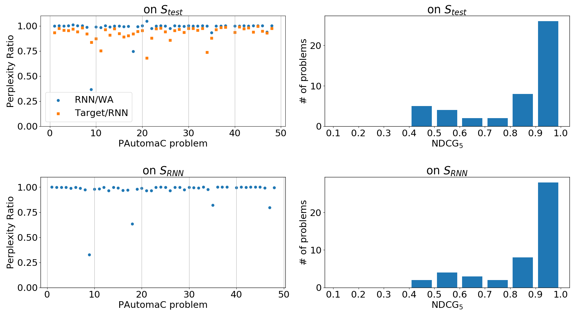
Figure 2: Perplexity ratio and NDCG₅ for synthetic problems on the 2 evaluation sets. Top-left plot shows ratios $\mbox{Perplexity}(P_{Target},P_{RNN})/\mbox{Perplexity}(P_{Target},P_{WA})$ in blue circles, and $\mbox{Perplexity}(P_{Target},P_{Target})/\mbox{Perplexity}(P_{Target},P_{RNN})$ in orange squares, both on the evaluation set $S_{test}$. Bottom-left plot shows ratio $\mbox{Perplexity}(P_{RNN},P_{RNN})/\mbox{Perplexity}(P_{RNN},P_{WA})$ on $S_{RNN}$. The right plots show the number of problems per NDCG₅ decile on the 2 evaluation sets.

The perplexity ratio shows a remarkable proximity between RNNs and WAs on all but 2 datasets (problems 9 and 18). In addition, this closeness between the 2 distributions does not seem to depend on the quality of the learning process, given by the perplexity ratio between the PAutomaC target model and the RNN. In particular, we can notice that problems 11, 21 and 34 have a low Target/RNN perplexity ratio, whereas RNN/WA is closed to the optimum, meaning that WA extraction works also well for poor RNN performances.

Regarding the distribution of NDCG₅ scores over 48 PAutomaC problems, we note that a large majority of the WA score higher than $0.9$ and about $70\%$ of problems with a score higher than $0.8$. This indicates that the WA estimations of next symbol probability are close to the RNN outputs.

6.2 Influence of the hyper-parameters

We analyze in this section the impact of the sizes of $\mathcal{P}$ and $\mathcal{S}$, as well as the rank for WA extraction on 2 synthetic and the 2 real datasets.

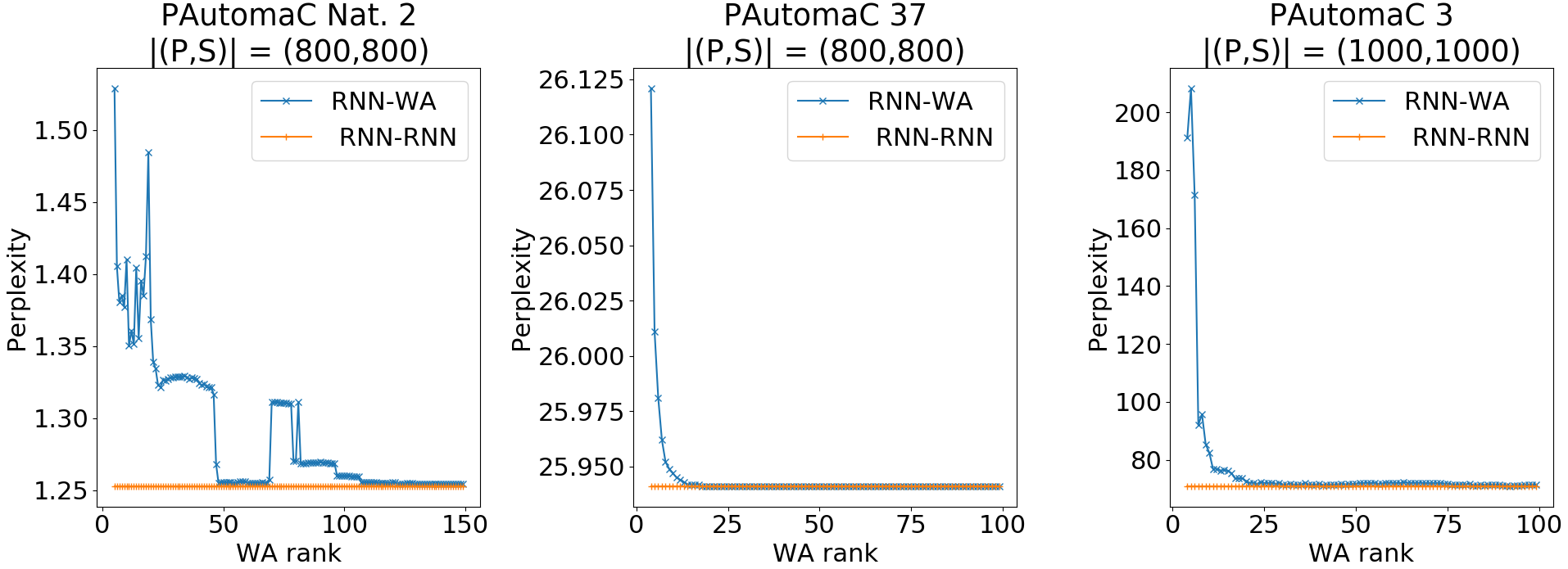
Figure 3: Influence of the rank parameter on the perplexity of 3 problems. PAutomaC Nat. 2 is the second real dataset presented in Section 5.2. PAutomaC 37 and PAutomaC 3 both correspond to a PFA target: the first one has 69 states on 8 symbols, the second 25 on 4.

Figure 3 shows the influence of rank on the quality of extracted WA, measured by the perplexity. We give both $\mbox{Perplexity}(P_{RNN},P_{RNN})$ and $\mbox{Perplexity}(P_{RNN},P_{WA})$. We notice that $\mbox{Perplexity}(P_{RNN},P_{RNN})$ corresponds to the RNN’s entropy, that is, the best possible score. We do not show results with rank values less than 5 in order to make the plots readable: for instance, the perplexity at rank 1 was higher than 20, for PAutomaC Nat. 2.

As expected, it appears that the higher the rank is, the better the quality of WA extraction becomes. Notice however that reasonable perplexity is obtained for small rank values. Our extracted WAs seem almost optimal with as few as 25 states.

On real problem PAutomaC Nat. 2, the quality of the extracted WA behaves more chaotically with rank variations, but still tends to converge to the optimum. We notice that variations are negligible since a perplexity of $1.35$ is already acceptable when the best possible is $1.25$.

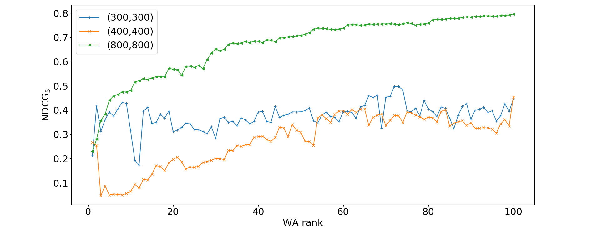
Figure 4: Influence of the size of the basis and the rank on NDCG₅ for problem SPiCe 4 (NLP). Each curve correspond to a different size of basis.

Figure 4 illustrates the impact of the size of the basis $\mathcal{B}$ and of the rank used to extract the WA. It appears that the quality of the WA approximation, measured in terms of NDCG₅, seems to increase with the number of prefixes and suffixes in the basis. The difference between configurations (300,300) and (400,400) is not significant, but doubling the basis size significantly improves the NDCG₅ score. This suggest that using even a larger basis might be useful on some tasks.

7 Discussion

Experiments show that our approach allows good approximations of black boxes, demonstrating that the linear projection defined by a WA can be close to the non-linear one of a RNN. Furthermore, we want to emphasize the fact that we dis not chose the most favorable framework: for instance, using RNNs to generate the basis could lead to better suited basis and thus to better approximation (for this future work, we may need RNNs specifically trained to generate sequences [Gra13] to avoid the autoregressive behavior). Using larger bases could also allow better results as our experiments tend to show (see Figure 4): this was not doable in reasonable time using our configuration (CPU, 4 cores, ~25Go RAM) but it is likely to not be a problem on state-of-the-art computers.

It is also worth noticing that, though we tested it on probabilistic models, the algorithm works on any black boxes that assign real values to sequences (or that can emulate this scheme, like the RNNs of our experiments) since WAs are not limited to probability distributions.

Another point that needs to be discussed is the interpretability of WAs: though they admit a graphical representation and are widely used in many fields, their non-deterministic nature can make them hard to read when the number of states increases. A first answer to that remark is that the algorithm described in this paper depends on a parameter, the rank, that can be tweaked: as the approximations for small rank values are already of acceptable quality, one can prefer readability to performance and chose a small rank value to obtain a small WA (see the example of a low rank extracted WA in Appendix). Our algorithm can then be seen as a way to compute a limited development of a black box function into WAs: by fixing the rank, one decides how detailed, and thus how close to the learned model, the extracted WA has to be.

A second answer to that point is that computing a weight (or the probability of the next symbol) is less expensive with WAs than with black boxes like RNNs. Indeed, the computation requires only matrix products, one per symbol in the input sequence, while non-linear models necessitate for each symbol several such products and the computation of non-linear functions. This is why the proposed algorithm share characteristics with distillation processes [HVD15]: from a complex, computationally costly model, it generates a simpler and more efficient one whose abilities are comparable.

Acknowledgements.

We want to thanks François Denis and Guillaume Rabusseau for fruitful discussions on WA and Benoit Favre for his help on RNN.

Appendix

Example of an extracted WA

Figure 5 gives the graphical representation on a WA extracted from a RNN trained on PAutomaC problem 24. This is not the best obtained WA on that dataset, but the metrics show that it is still a good approximation of the RNN.

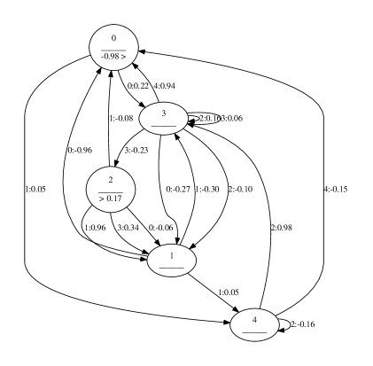
Figure 5: WA extracted for problem 24, at rank 5, with basis size 800x800. Its perplexity ratio is $0.99849$ while its NDCG₅ is 0.99848. Input weights are given on state before the $>$ symbol, while output ones appear after $>$. Transitions with absolute weight under 0.05 are not shown.

Metrics for best parameters

Figures 6, 7, 8, and 9 are analogues of Figure 2 where the best parameters for only one of the experimental condition is given. For instance, Figure 6 gives the perplexity ratios and the NDCG₅ on the two evaluation sets for the parameters allowing the best perplexity ratio on $S_{test}$.

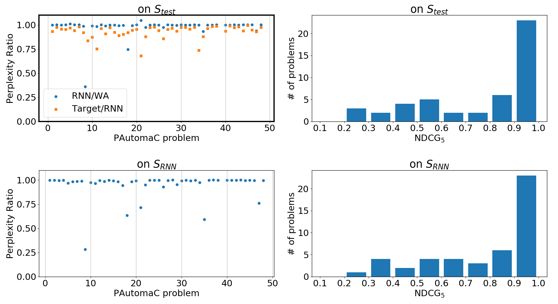
Figure 6: Perplexity ratio and NDCG₅ for the PAutomaC problems on the 2 evaluation sets using the parameter scoring the best perplexity ratio on $S_{test}$.

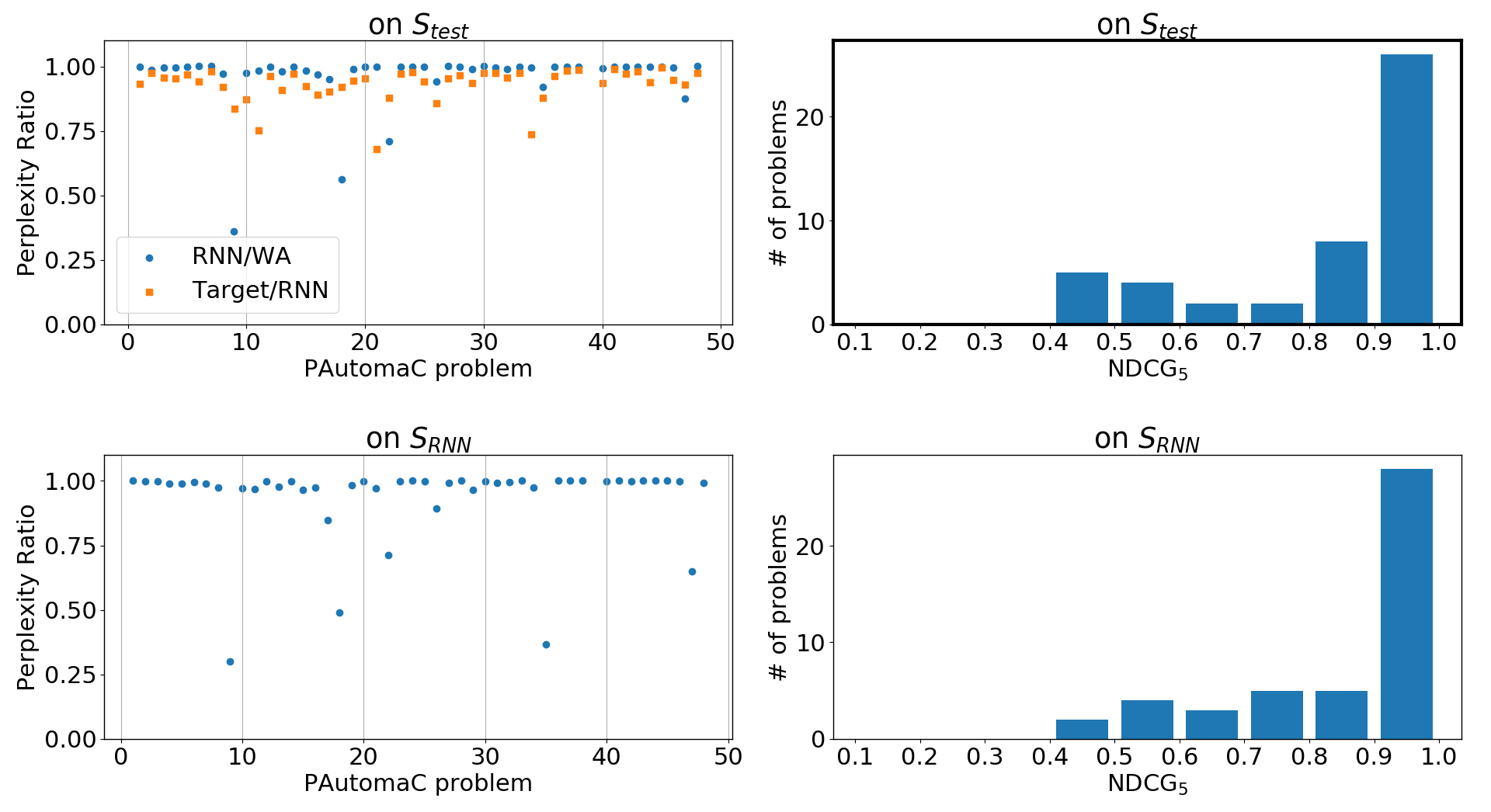
Figure 7: Perplexity ratio and NDCG₅ for the PAutomaC problems on the 2 evaluation sets using the parameter scoring the best NDCG on $S_{test}$.

Figure 8: Perplexity ratio and NDCG₅ for the PAutomaC problems on the 2 evaluation sets using the parameter scoring the best perplexity ratio on $S_{RNN}$.

Figure 9: Perplexity ratio and NDCG₅ for the PAutomaC problems on the 2 evaluation sets using the parameter scoring the best NDCG on $S_{RNN}$.

Influence of WA negative weights

A known and intensively studied [DE08, BD11, BCLQ14, ABDE17, BM18] behavior of Weighted Automata is their ability to assign negative weights to some strings. This is the counter-part of their great expressive power: when the Hankel matrix is not complete, or when its rank is not finite, or when its values are too noisy, the obtained WA might not represent exactly a probability distribution. It is important to understand that the absolute value of a negative weight does not carry any semantic: a negative weight for a WA approximating a probability distribution is exactly equivalent to having a probability of $0$.

This has no impact on the computation of NDCG, but it causes problem for the one of the perplexity since one needs to compute $\log(P_{WA}(w))$. As it cannot be replaced by $0$ either, we follow a commonly accepted path and chose to replace all negative values by a tiny $\epsilon$. In the experiments presented here, we set $\epsilon=10^{-30}$.

Figures 10 and 11 gives the evolution of the perplexity and the KL-divergence, respectively, when the rank increases on 3 different datasets, together with the percentage of epsilon use. On PAutomaC 37, almost no element of the evaluation is given a negative weight, whatever the rank is. On PAutomaC 3, the number of zeros rapidly decreases and tends to stabilize around $10\%$, which is an usually accepted rate.

On PAutomaC Natural Problem 2, the number of zeros increases with the rank, finishing above the $40\%$ rate for large rank values. However, the perplexity is not affected since it stays close to the best possible perplexity (the one of the RNN, given by the flat orange line). The natural explanation is that epsilons are given to extremely unlikely strings in the RNN. Indeed, if the WA assigns a negative weight to a string $w$, $\epsilon$ is use for $P_{WA}(w)$, which means that $log(P_{WA})$ is negative with a huge absolute value. As $\mbox{Perplexity}(\{w\})=2^{-P_{RNN}(w)log(P_{WA})}$, if $P_{RNN}(w)$ is not exceptionally small, then this perplexity would be extremely high, inexorably damaging the overall perplexity (it is not uncommon to witness models with perplexity over a million on some benchmarks). The fact that it does not happen here implies that $P_{RNN}(w)$ has to be small for strings of negative weights. Therefore, by assigning a zero probability to these strings, the WA realizes a good approximation of the RNN.

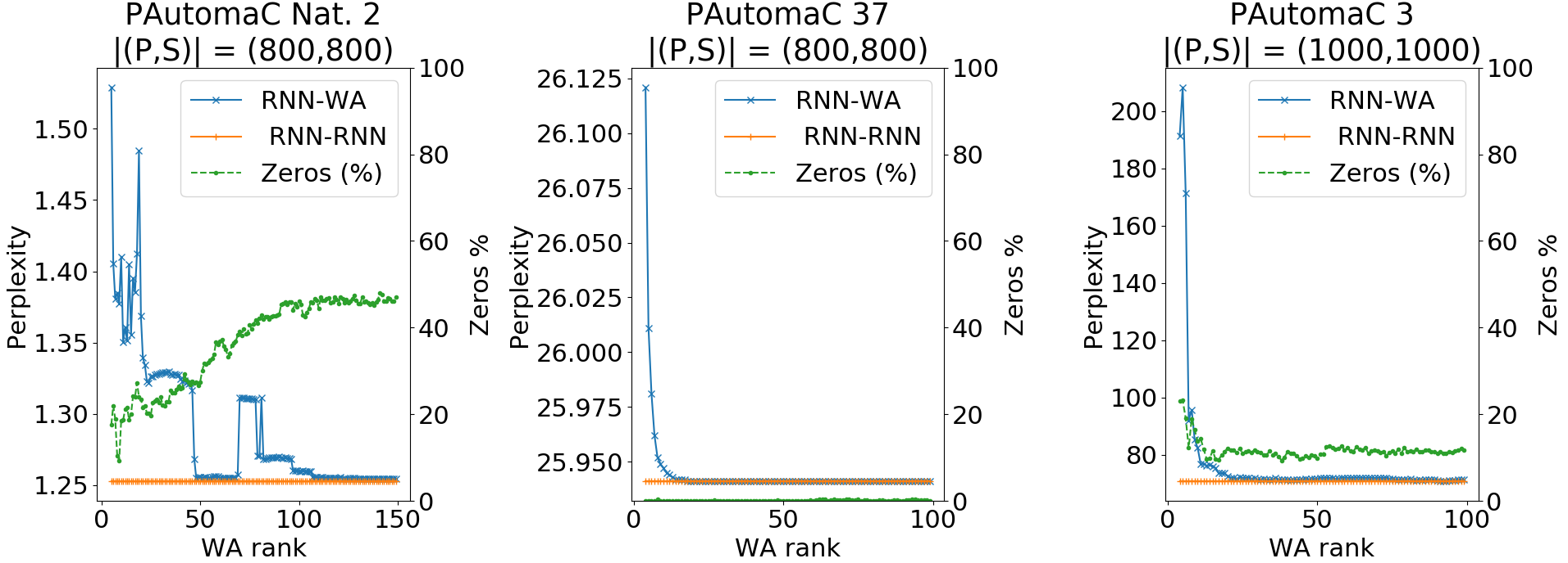
Figure 10: Influence of the rank parameter on the perplexity of 3 datasets, together with the number of zeros.

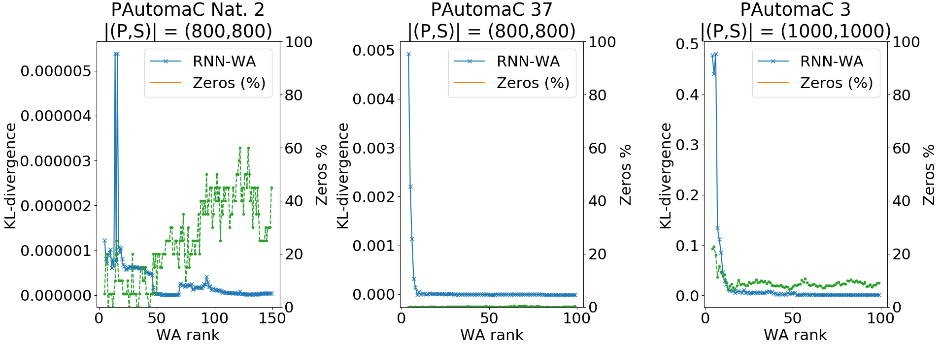
Figure 11: Influence of the rank parameter on the Kullback-Leibler divergence of 3 datasets, together with the number of zeros.

WER and NDCG₁

Figure 12 shows the best WER and NDCG₁ obtained on the evaluation sets on the synthetic problems.

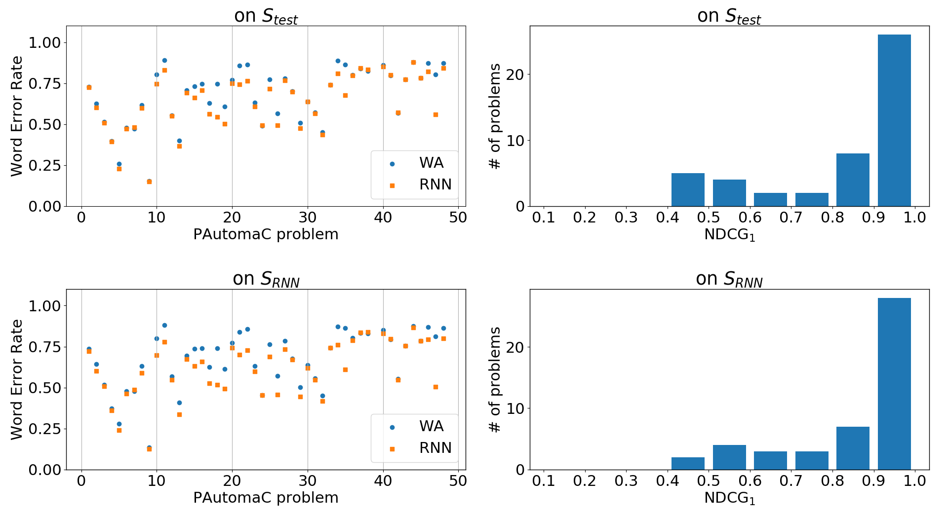
Figure 12: Results of WER and NDCG₁ with best parameters for each task and each PAutomaC problem.

Best extraction parameters on PAutomaC

Tables 1 and 2 give, for each problem of the PAutomaC dataset, the extraction parameters that obtain the best corresponding metric on $S_{test}$ and $S_{RNN}$, respectively. Columns Rank and $(P,S)$ contain respectively the rank value and the size of the basis that achieve the Value. Column Zeros gives the percentage of negative weights obtained when parsing a string of the evaluation set with the WA (see discussion about Figure 10 for details on that matter).

Pb.	Perplexity Ratio				NDCG5
#	Rank	(P,S)	Value	Zeros	Rank	(P,S)	Value
1	32	(1400,1400)	1.00009	4.2 %	96	(1400,1400)	0.95324
2	10	(1400,1400)	1.00162	2.2 %	12	(1400,1400)	0.92548
3	71	(800,800)	1.00012	5.0 %	75	(1400,1400)	0.99268
4	79	(800,800)	1.00073	2.1 %	42	(800,800)	0.99615
5	49	(800,800)	1.01140	0.6 %	51	(800,800)	0.98552
6	80	(1400,1400)	1.00114	6.5 %	57	(1400,1400)	0.98719
7	18	(800,800)	1.00296	0.0 %	17	(800,800)	0.99654
8	100	(1000,1000)	0.98765	15.2 %	100	(1400,1400)	0.91531
9	16	(1400,1400)	0.36845	24.6 %	19	(1400,1400)	0.79179
10	96	(1000,1000)	0.99008	30.5 %	39	(1400,1400)	0.71537
11	99	(1400,1400)	0.98284	36.4 %	98	(1400,1400)	0.61458
12	60	(1000,1000)	1.00044	8.6 %	35	(1400,1400)	0.97362
13	100	(1400,1400)	0.99040	8.0 %	58	(1400,1400)	0.97375
14	83	(800,800)	0.99967	5.0 %	47	(1000,1000)	0.94324
15	62	(1000,1000)	0.99979	23.0 %	32	(1400,1400)	0.76211
16	96	(1000,1000)	0.99283	19.3 %	88	(1000,1000)	0.83098
17	27	(1000,1000)	0.99520	14.3 %	28	(1000,1000)	0.83255
18	88	(1400,1400)	0.74500	24.2 %	95	(1000,1000)	0.59521
19	96	(1400,1400)	0.99375	18.3 %	100	(1400,1400)	0.83020
20	16	(1000,1000)	1.00102	30.1 %	65	(1000,1000)	0.90750
21	12	(800,800)	1.04705	37.1 %	69	(1400,1400)	0.54177
22	77	(1400,1400)	0.97386	36.6 %	97	(800,800)	0.57218
23	56	(1400,1400)	1.00000	9.4 %	76	(1400,1400)	0.94410
24	15	(800,800)	1.00030	0.0 %	39	(800,800)	0.99999
25	99	(800,800)	0.99996	17.0 %	95	(1400,1400)	0.81833
26	100	(1000,1000)	0.97447	14.6 %	89	(1400,1400)	0.88117
27	27	(1400,1400)	1.00174	11.9 %	21	(1000,1000)	0.87799
28	65	(1400,1400)	1.00000	3.3 %	95	(1400,1400)	0.98394
29	71	(1400,1400)	0.99554	7.8 %	95	(1400,1400)	0.95355
30	21	(1000,1000)	1.00051	3.5 %	43	(1400,1400)	0.96598
31	38	(800,800)	1.00000	3.2 %	68	(1400,1400)	0.98993
32	86	(1000,1000)	0.99836	5.1 %	98	(1400,1400)	0.97969
33	8	(1400,1400)	1.00046	0.9 %	71	(1000,1000)	0.99381
34	96	(1400,1400)	0.99867	41.0 %	97	(1400,1400)	0.57356
35	84	(800,800)	0.93308	37.3 %	77	(1400,1400)	0.44417
36	14	(1000,1000)	1.00008	10.0 %	91	(1400,1400)	0.95274
37	11	(800,800)	1.00000	0.0 %	98	(1400,1400)	0.99914
38	5	(1000,1000)	1.00028	1.5 %	82	(1400,1400)	0.99774
40	84	(1000,1000)	0.99959	24.0 %	99	(1400,1400)	0.82376
41	6	(800,800)	1.00007	0.0 %	85	(800,800)	0.99998
42	8	(1000,1000)	1.00158	0.2 %	19	(800,800)	0.99515
43	11	(800,800)	1.00003	0.0 %	74	(800,800)	0.99999
44	5	(1000,1000)	1.00064	2.4 %	39	(1000,1000)	0.94511
45	2	(800,800)	1.00021	0.4 %	62	(1400,1400)	0.99904
46	33	(1400,1400)	1.00143	34.2 %	64	(1400,1400)	0.64332
47	84	(1400,1400)	0.93862	31.3 %	57	(1400,1400)	0.48529
48	15	(800,800)	1.00154	23.5 %	52	(1400,1400)	0.72140

Table 1: Parameters for best obtained WA for each PAutomaC problems on $S_{test}$

Pb.	Perplexity Ratio				NDCG5
#	Rank	(P,S)	Value	Zeros	Rank	(P,S)	Value
1	90	(1400,1400)	0.99995	6.8 %	91	(1400,1400)	0.95030
2	65	(800,800)	0.99972	3.1 %	12	(1400,1400)	0.92548
3	92	(1000,1000)	0.99756	7.7 %	98	(1400,1400)	0.99232
4	94	(800,800)	0.99901	1.9 %	54	(1400,1400)	0.99407
5	32	(1000,1000)	0.99064	0.1 %	51	(800,800)	0.98552
6	100	(1400,1400)	0.99912	3.1 %	35	(1400,1400)	0.98669
7	29	(800,800)	0.98952	0.6 %	17	(800,800)	0.99654
8	100	(1400,1400)	0.97525	12.5 %	98	(1400,1400)	0.91287
9	16	(1400,1400)	0.31197	24.6 %	22	(1400,1400)	0.79165
10	70	(1400,1400)	0.97911	32.0 %	40	(1400,1400)	0.71336
11	66	(1400,1400)	0.98303	34.4 %	88	(1400,1400)	0.60401
12	93	(1400,1400)	0.99879	7.2 %	34	(1400,1400)	0.96598
13	89	(1000,1000)	0.96508	10.4 %	56	(1400,1400)	0.96758
14	53	(1400,1400)	0.99683	7.0 %	9	(1000,1000)	0.93522
15	100	(1400,1400)	0.99204	25.6 %	28	(1400,1400)	0.75812
16	97	(1400,1400)	0.96902	25.0 %	97	(1000,1000)	0.82633
17	72	(1000,1000)	0.97144	25.6 %	26	(1400,1400)	0.80701
18	88	(1400,1400)	0.63316	24.2 %	95	(1000,1000)	0.59521
19	99	(800,800)	0.97982	23.2 %	100	(1400,1400)	0.83020
20	74	(800,800)	0.98953	30.8 %	98	(1000,1000)	0.88840
21	85	(1000,1000)	0.96581	39.9 %	69	(1400,1400)	0.54177
22	95	(1000,1000)	0.96631	39.7 %	100	(1000,1000)	0.56973
23	57	(800,800)	0.99905	13.3 %	68	(1400,1400)	0.93060
24	24	(1000,1000)	0.99993	0.0 %	32	(800,800)	0.99997
25	95	(1000,1000)	0.99921	19.6 %	99	(1400,1400)	0.81832
26	90	(1000,1000)	0.96623	14.1 %	81	(1400,1400)	0.87139
27	100	(1000,1000)	0.99796	18.6 %	63	(1400,1400)	0.85724
28	87	(800,800)	0.99932	12.0 %	97	(1400,1400)	0.98082
29	81	(1400,1400)	0.97509	7.3 %	97	(1400,1400)	0.94998
30	91	(1400,1400)	0.99976	5.3 %	80	(1000,1000)	0.95873
31	26	(1000,1000)	0.99650	4.3 %	95	(1400,1400)	0.98882
32	97	(1000,1000)	0.99303	9.5 %	99	(1400,1400)	0.97968
33	73	(1000,1000)	0.99998	11.5 %	77	(1000,1000)	0.98977
34	100	(1400,1400)	0.97584	37.4 %	92	(1400,1400)	0.56693
35	87	(1400,1400)	0.82007	40.2 %	62	(800,800)	0.44097
36	57	(800,800)	0.99997	11.3 %	100	(1400,1400)	0.95238
37	18	(800,800)	1.00000	0.1 %	100	(1400,1400)	0.99914
38	19	(1400,1400)	1.00000	7.2 %	93	(1400,1400)	0.99760
40	75	(800,800)	0.99560	27.6 %	100	(1400,1400)	0.82201
41	15	(800,800)	1.00000	0.0 %	83	(800,800)	0.99997
42	80	(800,800)	0.99968	6.4 %	7	(1000,1000)	0.99442
43	17	(1400,1400)	1.00000	0.0 %	72	(800,800)	0.99998
44	24	(800,800)	1.00000	6.1 %	99	(1000,1000)	0.94282
45	19	(1400,1400)	1.00000	0.2 %	4	(1400,1400)	0.99885
46	46	(1000,1000)	0.99110	37.2 %	72	(1400,1400)	0.64257
47	100	(1400,1400)	0.79781	33.7 %	57	(1400,1400)	0.48529
48	51	(800,800)	0.99561	37.6 %	50	(1400,1400)	0.71464

Table 2: Parameters for best obtained WA for each PAutomaC problems on $S_{RNN}$

References

- [ABDE17] D. Arrivault, D. Benielli, F. Denis, and R. Eyraud. Scikit-SpLearn: a toolbox for the spectral learning of weighted automata compatible with scikit-learn. In Conférence francophone en Apprentissage, 2017.
- [Aeaea15] M. Abadi, et al., and et al. TensorFlow: Large-scale machine learning on heterogeneous systems, 2015. Software available from tensorflow.org.
- [Bai11] R. Bailly. Méthodes spectrales pour l’inférence grammaticale probabiliste de langages stochastiques rationnels. PhD thesis, 2011. Aix-Marseille Univ.
- [BCLQ14] B. Balle, X. Carreras, F. Luque, and A. Quattoni. Spectral learning of weighted automata. Machine Learning, 96(1-2):33–63, 2014.
- [BCNM06] C. Buciluǎ, R. Caruana, and A. Niculescu-Mizil. Model compression. In Proc. of the ACM SIGKDD International Conference on Knowledge Discovery and Data Mining, pages 535–541, 2006.
- [BD11] R. Bailly and F. Denis. Absolute convergence of rational series is semi-decidable. Inf. Comput., 209(3):280–295, 2011.
- [BDR09] R. Bailly, F. Denis, and L. Ralaivola. Grammatical inference as a principal component analysis problem. In International Conference on Machine Learning, pages 33–40, 2009.
- [BEL+17] B. Balle, R. Eyraud, F. M. Luque, A. Quattoni, and S. Verwer. Results of the sequence prediction challenge (SPiCe): a competition on learning the next symbol in a sequence. In Proc. of the International Conference on Grammatical Inference, volume 57 of PMLR, pages 132–136, 2017.
- [BM18] B. Balle and M. Mohri. Generalization bounds for learning weighted automata. Theor. Comput. Sci., 716:89–106, 2018.
- [C+15] F. Chollet et al. Keras. https://keras.io, 2015.
- [CP71] J.W. Carlyle and A. Paz. Realizations by stochastic finite automata. Journal of Computer and System Sciences, 5(1):26 – 40, 1971.
- [CRAOMGO13] A. Cruz-Roa, J. Arevalo Ovalle, A. Madabhushi, and F. González Osorio. A deep learning architecture for image representation, visual interpretability and automated basal-cell carcinoma cancer detection. In Medical Image Computing and Computer-Assisted Intervention, pages 403–410, 2013.
- [CvMG+14] K. Cho, B. van Merriënboer, Ç. Gülçehre, D. Bahdanau, F. Bougares, H. Schwenk, and Y. Bengio. Learning phrase representations using rnn encoder–decoder for statistical machine translation. In Proc. of the Conference on Empirical Methods in Natural Language Processing, pages 1724–1734. ACL, 2014.
- [DE08] F. Denis and Y. Esposito. On rational stochastic languages. Fundamenta Informaticae, 86(1-2):41–77, 2008.
- [DKV09] M. Droste, W. Kuich, and H. Vogler. Handbook of Weighted Automata. Springer Publishing Company, Incorporated, 1st edition, 2009.
- [DLML10] E. S. Dimitrova, M. P. Vera Licona, J. McGee, and R. Laubenbacher. Discretization of time series data. Journal of Computational Biology, 17(6):853–868, 2010.
- [DVK17] F. Doshi-Velez and B. Kim. Towards a rigorous science of interpretable machine learning. CoRR, abs/1702.08608, 2017.
- [Fli74] M. Flies. Matrice de hankel. Journal de Mathématique Pures et Appliquées, 5:197–222, 1974.
- [Fre14] A. A. Freitas. Comprehensible classification models: A position paper. SIGKDD Explor. Newsl., 15(1):1–10, 2014.
- [GDP16] GDPR. Regulation (EU) 2016/679 of the European Parliament and of the Council of 27 April 2016 on the protection of natural persons with regard to the processing of personal data and on the free movement of such data (General Data Protection Regulation). Official Journal of the European Union, L119:1–88, May 2016.
- [GMC+92] C. L. Giles, C. B. Miller, D. Chen, H. H. Chen, G. Z. Sun, and Y. C. Lee. Learning and extracting finite state automata with second-order recurrent neural networks. Neural Computation, 4(3):393–405, 1992.
- [GMT+18] R. Guidotti, A. Monreale, F. Turini, D. Pedreschi, and F. Giannotti. A survey of methods for explaining black box models. CoRR, abs/1802.01933, 2018.
- [Gra13] A. Graves. Generating sequences with recurrent neural networks. CoRR, abs/1308.0850, 2013.
- [HKZ09] D. Hsu, S. Kakade, and T. Zhang. A spectral algorithm for learning hidden markov models. In Conference on Computational Learning Theory, 2009.
- [HS97] S. Hochreiter and J. Schmidhuber. Long short-term memory. Neural Computation, 9(8):1735–1780, 1997.
- [HVD15] G. Hinton, O. Vinyals, and J. Dean. Distilling the knowledge in a neural network. In NIPS Deep Learning and Representation Learning Workshop, 2015.
- [Jac05] H. Jacobsson. Rule extraction from recurrent neural networks: A taxonomy and review. Neural Comput., 17(6):1223–1263, 2005.
- [Lip16] Z. C. Lipton. The mythos of model interpretability. CoRR, abs/1606.03490, 2016.
- [LM12] G. Lecorvé and P. Motlícek. Conversion of recurrent neural network language models to weighted finite state transducers for automatic speech recognition. In Proc. of the Conference of the International Speech Communication Association, pages 1668–1671, 2012.
- [Moh09] M. Mohri. Handbook of Weighted Automata, chapter Weighted Automata Algorithms, pages 213–254. Springer Berlin Heidelberg, 2009.
- [Moo20] E. H. Moore. On the reciprocal of the general algebraic matrix. Bulletin of the American Mathematical Society, 26:394–395, 1920.
- [MSM94] M. P. Marcus, B. Santorini, and M. A. Marcinkiewicz. Building a large annotated corpus of english: The penn treebank. Computational Linguistics, 19(2):313–330, 1994.
- [OG96] C. W. Omlin and C. L. Giles. Extraction of rules from discrete-time recurrent neural networks. Neural Networks, 9(1):41 – 52, 1996.
- [OSJ+18] C. Olah, A. Satyanarayan, I. Johnson, S. Carter, L. Schubert, K. Ye, and A. Mordvintsev. The building blocks of interpretability. Distill, 2018.
- [QCG17] A. Quattoni, X. Carreras, and M. Gallé. A maximum matching algorithm for basis selection in spectral learning. In Proc. of the 20th International Conference on Artificial Intelligence and Statistics, volume 54 of PMLR, pages 1477–1485, 2017.
- [RBP17] G. Rabusseau, B. Balle, and J. Pineau. Multitask spectral learning of weighted automata. In Advances in Neural Information Processing Systems, pages 2585–2594, 2017.
- [RSG16] M. Túlio Ribeiro, S. Singh, and C. Guestrin. "why should I trust you?": Explaining the predictions of any classifier. In Proc. of the International Conference on Knowledge Discovery and Data Mining, pages 1135–1144, 2016.
- [Sak09] J. Sakarovitch. Rational and Recognisable Power Series, pages 105–174. 2009.
- [SH17] C. Shibata and J. Heinz. Predicting sequential data with LSTMs augmented with strictly 2-piecewise input vectors. In Proc. of the International Conference on Grammatical Inference, volume 57 of PMLR, pages 137–142, 2017.
- [SVL14] I. Sutskever, O. Vinyals, and Q. V. Le. Sequence to sequence learning with neural networks. CoRR, abs/1409.3215, 2014.
- [VdWW11] S. Verwer, M. de Weerdt, and C. Witteveen. Learning driving behavior by timed syntactic pattern recognition. In Proc. of the 22nd International Joint Conference on Artificial Intelligence, pages 1529–1534, 2011.
- [VEdlH14] S. Verwer, R. Eyraud, and C. de la Higuera. PAutomaC: a probabilistic automata and hidden markov models learning competition. Machine Learning, 96(1-2):129–154, 2014.
- [WGY18] G. Weiss, Y. Goldberg, and E. Yahav. Extracting automata from recurrent neural networks using queries and counterexamples. In Proc. of the International Conference on Machine Learning, volume 80, pages 5244–5253. PMLR, 2018.
- [WZI+17] Q. Wang, K. Zhang, A. G. Ororbia II, X. Xing, X. Liu, and C. L. Giles. An empirical evaluation of recurrent neural network rule extraction. CoRR, abs/1709.10380, 2017.