Improving Generalization of Sequence Encoder-Decoder Networks for
Inverse Imaging of Cardiac Transmembrane Potential

Abstract

Deep learning models have shown state-of-the-art performance in many inverse reconstruction problems. However, it is not well understood what properties of the latent representation may improve the generalization ability of the network. Furthermore, limited models have been presented for inverse reconstructions over time sequences. In this paper, we study the generalization ability of a sequence encoder-decoder model for solving inverse reconstructions on time sequences. Our central hypothesis is that the generalization ability of the network can be improved by 1) constrained stochasticity and 2) global aggregation of temporal information in the latent space. First, drawing from analytical learning theory, we theoretically show that a stochastic latent space will lead to an improved generalization ability. Second, we consider an LSTM encoder-decoder architecture that compresses a global latent vector from all last-layer units in the LSTM encoder. This model is compared with alternative LSTM encoder-decoder architectures, each in deterministic and stochastic versions. The results demonstrate that the generalization ability of an inverse reconstruction network can be improved by constrained stochasticity combined with global aggregation of temporal information in the latent space.

Introduction

There has been an upsurge in the use of deep learning based methods in inverse problems in computer vision and medical imaging (?). Examples include image denoising (?), inpainting (?), super resolution (?) and image reconstructions in a variety of medical imaging modalities such as magnetic resonance imaging, X-ray, and computed tomography (?; ?; ?). A common deep network architecture for inverse reconstructions is a encoder-decoder network, which learns to encodes an input measurement into a latent representation that is then decoded into a desired inverse solution (?; ?). Despite significant successes of these models, two important questions remain relatively unexplored. First, it is not well understood what properties of the latent representation improve the generalization ability of the network. Second, existing works mostly focus on solving single-image problems, while limited models exist for solving inverse problems on image or signal sequences. The latter, however, is important because the incorporation of temporal information can often help alleviate the ill-posedness of an inverse reconstruction problem.

In this paper, we present a probabilistic sequence encoder-decoder model for solving inverse problems on time sequences. Central to the presented model is an emphasis on the generalization ability of the network in order to learn a general inverse mapping from the measurement to reconstruction results. Our main hypothesis is that the generalization ability of the sequence encoder-decoder network can be improved by the following two properties of the latent space: 1) constrained stochasticity, and 2) global aggregation of information throughout the long time sequence.

First, we theoretically show that using stochastic latent space during training helps to learn a decoder that is less sensitive to local changes in the latent space and that, based on analytical learning theory (?), leads to good generalization ability of the network . Second, while it is common in a sequence model to use the last unit of a recurrent encoder network for decoding, we hypothesize that – in the presence of long time sequences – the last hidden unit code may not be able to retain global information and may act as a bottleneck in information flow. This shares a fundamental idea with recent works in which alternative architectures were presented with attention mechanism to consider information from all the hidden states of long-short-term-memory (LSTM) networks (?; ?). Alternative strategies were also presented to back-propagate the loss through all hidden states addressing the issue of gradient vanishing (?; ?). Here, to arrive at a compact latent space that globally summarizes a long time sequence, we present an architecture (termed as svs) to combine and compress all LSTM units into a vector representation.

While the presented methodology applies for general sequence inverse problems, we test it on the problem of inverse reconstruction of cardiac transmembrane potential (TMP) sequence from high-density electrocardiogram (ECG) sequence acquired on the body surface (?; ?; ?). In this setting, the measurement at each time instant is a spatial potential map on the body surface, and the reconstruction output is a spatial potential map throughout the three-dimensional heart muscle. The problem at each time instant is severely ill-posed, and incorporating temporal information is recognized as a main approach to alleviate this issue.

To investigate the generalization ability of the presented model, we analyzed in-depth the benefits brought by each of the two key components within the presented model. In specific, we compared the presented svs architecture with two alternatives: one that decodes directly from the sequence produced by the LSTM encoder (termed as sss) and one that decodes from the output of the last unit of the LSTM encoder, as mostly commonly used in language models (termed as svs-L) (?). We also compared between deterministic and stochastic versions of svs and svs-L. The experiments results suggest that the generalization ability of the network in inverse reconstruction can be improved by constrained stochasticity combined with global aggregation of sequence information in the latent space. These findings may set a foundation for investigating the generalization ability of deep networks in sequence inverse problems and inverse problems in general.

Related Work

There is a large body of work in the the use of deep learning in inverse imaging in both general computer vision (?; ?; ?; ?; ?) and medical imaging (?; ?; ?). Some of these deep inverse reconstruction networks are based on an encoder-decoder structure (?; ?), similar to that investigated in this paper. Among these works in the domain of medical image reconstruction, the presented work is the closest to Automap (?), in that the output image is reconstructed directly from the input measurements without any domain-specific intermediate transformations. However, all of these works employ a deterministic architecture which, as we will show later, can be improved with the introduction of stochasticity. Nor do these existing works handle inverse reconstructions of images or signals over time sequences.

Different elements of the presented work are conceptually similar to several works across different domains of machine learning. The use of encoder-decoder architectures for sequential signals is related to existing works in language translation (?). However, we investigate an alternative global aggregation of sequence information by utilizing and compressing knowledge from all the units in the last layer of the LSTM encoder. This is in concept similar to the works in (?; ?), where information from all the units of an LSTM encoder are used for language translation. However, to our knowledge, no existing works have analyzed in-depth the difference in the generalization ability of sequence encoder-decoder models with respect to these different designs of the latent space.

The presented theoretical analysis of stochasticity in generalization utilizes analytical learning theory (?), which is fundamentally different from classical statistical learning theory in that it is strongly instance-dependent. While statistical learning theory deals with data-independent generalization bounds or data dependent bounds for certain hypothesis space of problems, analytical learning theory provides the bound on how well a model learned from a dataset should perform on true (unknown) measures of variable of interest. This makes it aptly suitable for measuring the generalization ability of a stochastic latent space for the given problem and data.

The presented work is related to variational autoencoder (VAE) in using stochastic latent space with regularization (?). Similarly, (?) present a sequence-to-sequence VAE based on LSTM encoder and decoders to generate coherent and diverse sentences from continuous sampling of latent code. However, it is not well understood why stochasticity of the latent space is so important. In this paper, we intend to provide a justification from the learning theory perspective. In addition, while VAE by nature is concerned with the reconstruction of the same input data, the presented network is concerned with the ill-posed problem of inverse signal/image reconstruction from their (often weak) measurements.

Preliminaries

Inverse Imaging of cardiac transmembrane potential (TMP)

Body-surface electrical potential is produced by TMP in the heart. Their mathematical relation is defined by the quasi-static approximation of electromagnetic theory (?) and, when solved on patient-specific heart-torso geometry, can be derived as (?):

$$\boldsymbol{y}=\boldsymbol{Hx}$$ (1)

where $\boldsymbol{y}$ denotes the body-surface potential map, $\boldsymbol{x}$ the 3D TMP map over the heart muscle, and $\boldsymbol{H}$ the measurement matrix specific to the heart-torso geometry of an individual.

The inverse reconstruction of $\boldsymbol{x}$ from $\boldsymbol{y}$ can be carried out at each time instant independently, which however is notoriously ill-posed since surface potential provides only a weak projection of the 3D TMP. A popular approach is thus to reconstruct the time sequence of TMP propagation over a heart beat, with various strategies to incorporate the temporal information to alleviate the ill-posedness of the problem (?; ?). Here, we examine the sequence setting, where $\boldsymbol{x}$ and $\boldsymbol{y}$ represents sequence matrices with each column denoting the potential map at one time instant. This problem has important clinical applications in supporting the diagnosis and treatment for diseases such as ischemia (?) and ventricular arrhythmia (?).

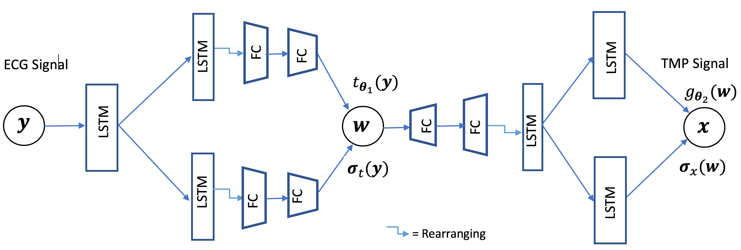
Figure 1: Presented svs stochastic architecture with mean and variance network in both encoder and decoder.

RNN and LSTM

Recurrent neural networks (RNN) (?; ?) generalize the traditional neural networks for sequential data by allowing passage of information over time. Compared to traditional RNNs, LSTM networks (?; ?) can better handle long term dependency in the data by architectural changes such as using a memory line called the cell state that runs throughout the whole sequence, the ability to forget information deemed irrelevant using a forget gate, and the ability to selectively update the cell state.

Variational Autoencoder (VAE)

VAE (?) is a probabilistic generative model that is typically trained by optimizing the variational lower bound of the data log likelihood. A VAE is distinctive from the traditional autoencoder in two aspects : 1) the use of stochastic latent space realized by sampling with a reparameterization trick, 2) the use of Kullback-Leibler (KL) divergence to regularize the latent distribution.

Methodology

We train a probabilistic sequence encoder-decoder network to learn to reconstruct the time sequence of TMP, $\boldsymbol{x}$, from input body-surface potential, $\boldsymbol{y}$. In a supervised setting, we maximize the log likelihood as follows:

$$\underset{\boldsymbol{\theta}}{argmax}\hskip 5.69046pt{E_{P(\boldsymbol{x},\boldsymbol{y})}\log p_{\boldsymbol{\theta}}(\boldsymbol{x}|\boldsymbol{y})}$$ (2)

where $P(\boldsymbol{x},\boldsymbol{y})$ is the joint distribution of the input-output pair. We introduce a latent random variable $\boldsymbol{w}$ and express the conditional distribution as:

$$p_{\boldsymbol{\theta}}(\boldsymbol{x}|\boldsymbol{y})=\int p_{\boldsymbol{\theta}_{2}}(\boldsymbol{x}|\boldsymbol{w})p_{\boldsymbol{\theta}_{1}}(\boldsymbol{w}|\boldsymbol{y})d\boldsymbol{w}$$ (3)

where $\boldsymbol{\theta}=\{\boldsymbol{\theta}_{1},\boldsymbol{\theta}_{2}\}$. We model both $p_{\boldsymbol{\theta}_{2}}(\boldsymbol{x}|\boldsymbol{w})$ and $p_{\boldsymbol{\theta}_{1}}(\boldsymbol{w}|\boldsymbol{y})$ with Gaussian distributions, with mean and variance parameterized by neural networks:

$$p_{\boldsymbol{\theta}_{1}}(\boldsymbol{w}|\boldsymbol{y})=\mathcal{N}(\boldsymbol{w}|\boldsymbol{t}_{\theta_{1}}(y),\boldsymbol{\sigma_{t}}^{2}(\boldsymbol{y}))$$ (4)

$$p_{\boldsymbol{\theta}_{2}}(\boldsymbol{x}|\boldsymbol{w})=\mathcal{N}(\boldsymbol{x}|\boldsymbol{g}_{\theta_{2}}(\boldsymbol{w}),\boldsymbol{\sigma_{x}}^{2}(\boldsymbol{w}))$$ (5)

where $\boldsymbol{\sigma_{x}}^{2}$ denotes a matrix of the same dimension as that of $\boldsymbol{x}$. We implicitly assume that each elements in $\boldsymbol{x}$ is independent and Gaussian with variance given by the corresponding element in $\boldsymbol{\sigma_{x}}^{2}$; and similarly for $\boldsymbol{w}$. Introduction of the latent random variable in the network allows us to constrain it in two means to improve the generalization ability of inverse reconstructions. First, we constrain the conditional distribution $p_{\boldsymbol{\theta}_{1}}(\boldsymbol{w}|\boldsymbol{y})$ to be close to an isotropic Gaussian distribution. Second, we design it to be a concise vector representation compressed from the whole input time sequence.

Regularized stochasticity

Drawing from the VAE (?), we regularize the latent space by constraining the conditional distribution $p_{\boldsymbol{\theta}_{1}}(\boldsymbol{w}|\boldsymbol{y})$ to be close to an isotropic Gaussian distribution. Training of the network can then be formulated as a constrained optimization problem as follows:

$$\textrm{minimize}-{E_{P(x,y)}\log\int p_{\boldsymbol{\theta}_{2}}}(\boldsymbol{x}|\boldsymbol{w})p_{\boldsymbol{\theta}_{1}}(\boldsymbol{w}|\boldsymbol{y})d\boldsymbol{w}$$

$$\textrm{such}\hskip 2.84544pt\textrm{that}\hskip 2.84544ptD_{KL}(p_{\boldsymbol{\theta}_{1}}(\boldsymbol{w}|\boldsymbol{y})||\mathcal{N}(\boldsymbol{w}|\boldsymbol{0},\boldsymbol{I}))<\delta$$ (6)

Using the method of Lagrange multipliers, we reformulate the objective function into:

$$\mathcal{L} =-{E_{P(x,y)}\log\Big{[}\int p_{\boldsymbol{\theta}_{2}}}(\boldsymbol{x}|\boldsymbol{w})p_{\boldsymbol{\theta}_{1}}(\boldsymbol{w}|\boldsymbol{y})d\boldsymbol{w}$$

$$+\lambda.(D_{KL}(p_{\boldsymbol{\theta}_{1}}(\boldsymbol{w}|\boldsymbol{y})||\mathcal{N}(\boldsymbol{w}|\boldsymbol{0},\boldsymbol{I}))-\delta)\Big{]}$$

$$\leq-{E_{P(x,y)}\Big{[}E_{w\sim p_{\boldsymbol{\theta}_{1}}(\boldsymbol{w}|\boldsymbol{y})\}}[\log p_{\boldsymbol{\theta}_{2}}}(\boldsymbol{x}|\boldsymbol{w})]$$

$$+\lambda.(D_{KL}(p_{\boldsymbol{\theta}_{1}}(\boldsymbol{w}|\boldsymbol{y})||\mathcal{N}(\boldsymbol{w}|\boldsymbol{0},\boldsymbol{I}))-\delta)\Big{]}$$ (7)

where the inequality in eq.(Regularized stochasticity) is due to Jensen’s inequality as the negative logarithm is a convex function. We use reparameterization $\boldsymbol{w}=\boldsymbol{t}+\boldsymbol{\sigma}_{t}\odot\boldsymbol{\epsilon}$ as described in (?) to compute the inner expectation in the first term. The KL divergence in the second term is analytically available for two Gaussian distributions. We thus obtain the upper bound for the loss function as:

$$\mathcal{L}\leq E_{P(\boldsymbol{x},\boldsymbol{y})}\Big{[}E_{\boldsymbol{\epsilon}\sim\mathcal{N}(\boldsymbol{0},\boldsymbol{I})}\Big{(}\sum_{i}\frac{1}{\boldsymbol{\sigma_{x}}_{i}^{2}}(x_{i}-g_{i}(\boldsymbol{t}+\boldsymbol{\sigma_{t}}\odot\boldsymbol{\epsilon}))^{2}$$

$$+\log\boldsymbol{\sigma_{x}}_{i}^{2}\Big{)}+\lambda.D_{KL}(p_{\boldsymbol{\theta}_{1}}(\boldsymbol{w}|\boldsymbol{y})||\mathcal{N}(\boldsymbol{w}|\boldsymbol{0},\boldsymbol{I}))\Big{]}+constant$$ (8)

where $g_{i}$ is the $i^{th}$ function mapping latent variable to the $i^{th}$ element of mean of $\boldsymbol{x}$, such that $\boldsymbol{g}_{\boldsymbol{\theta}_{2}}=[g_{1},g_{2}...g_{U}]$.

Global aggregation of sequence information

In sequence inverse problems where the measurement at each time instant provides only a weak projection of the reconstruction solution, utilizing the temporal information in the sequence becomes important for better inverse reconstructions. This motivate us to design an architecture that can distill from the input sequence a global, time-invariant, and low dimensional latent representation from which the entire TMP sequence can be reconstructed.

To do so, we present an architecture with two LSTM networks followed by two fully connected neural networks (FC), each respectively for the mean and variance in the encoder network. The decoder then consists of two FC followed by two LSTM networks for the mean and variance of the output. In the encoder, each LSTM decreases spatial dimensions while keeping temporal dimensions constant; the last-layer outputs from all the units in each LSTM are reshaped into a vector, the length of which is decreased by the FC. The structure and dimension of the decoder mirrors that of the encoder. The overall architecture of the presented network is illustrated in Fig. 1.

Encoder-Decoder Learning from the Perspective of Analytical Learning Theory

In this section we look at the encoder-decoder inverse reconstructions from the analytical learning theory (?). We start with a deterministic latent space setting and then show that having a stochastic latent space with regularization helps in generalization.

Let $\boldsymbol{z}=(\boldsymbol{y},\boldsymbol{x})$ be an input-output pair, and let $D_{n}=\{\boldsymbol{z}^{(1)},\boldsymbol{z}^{(2)},...,\boldsymbol{z}^{(n)}\}$ denote the total set of training and validation data and $Z_{m}\subset D_{n}$ be a validation set. During training, a neural network learns the parameter $\boldsymbol{\theta}$ by using an algorithm $\mathcal{A}$ and dataset $D_{n}$, at the end of which we have a mapping $h_{\mathcal{A}(D_{n})}(.)$ from $\boldsymbol{y}$ to $\boldsymbol{x}$. Typically, we stop training when the model performs well in the validation set. To evaluate this performance, we define a loss function based on our notion of goodness of prediction as $\ell(\boldsymbol{x},h_{\mathcal{A}(D_{n})}(\boldsymbol{y}))$. The average validation error is given by ${E_{Z_{m}}\ell(\boldsymbol{x},h_{\mathcal{A}(D_{n})}(\boldsymbol{y}))}$.

However, there exists a gap between how well the model performs in the validation set versus in the true distribution of the input-output pair; this gap is called the generalization gap. To be precise let $(\mathcal{Z},\mathcal{S},\mu)$ be a measure space with $\mu$ being a measure on $(\mathcal{Z},\mathcal{S})$. Here, $\mathcal{Z}=\mathcal{Y}\times\mathcal{X}$ denotes the input-output space of all the observations and inverse solutions. The generalization gap is given by:

$${E_{\mu}\ell(\boldsymbol{x},h_{\mathcal{A}(D_{n})}(\boldsymbol{y}))}-{E_{Z_{m}}\ell(\boldsymbol{x},h_{\mathcal{A}(D_{n})}(\boldsymbol{y}))}$$ (9)

Note that this generalization gap depends on the specific problem instance. Theorem 1 (?) provides an upper bound on equation (9) in terms of data distribution in the latent space and properties of the decoder.

Theorem 1 ((?)).

For any $\ell$, let $(\mathcal{T},f)$be a pair such that $\mathcal{T}:(\mathcal{Z},\mathcal{S})\rightarrow([0,1]^{d},\mathcal{B}([0,1]^{d}))$ is a measurable function, $f:([0,1]^{d},\mathcal{B}([0,1]^{d}))\rightarrow(\mathbb{R},\mathcal{B}(\mathbb{R}))$ is of bounded variation as $V[f]<\infty$, and $\ell(\boldsymbol{x},h(\boldsymbol{y}))=(f\circ\mathcal{T})(\boldsymbol{z})\forall\boldsymbol{z}\in\mathcal{Z}$, where $\mathcal{B}(A)$ indicates the Borel $\sigma$- algebra on $A$. Then for any dataset pair $(D_{m},Z_{m})$ and any $\ell(\boldsymbol{x},h_{\mathcal{A}(D_{n})}(\boldsymbol{y}))$,

$${E_{\mu}\ell(\boldsymbol{x},h_{\mathcal{A}(D_{m})}(\boldsymbol{y}))}-{E_{Z_{m}}\ell(\boldsymbol{x},h_{\mathcal{A}(D_{n})}(\boldsymbol{y}))}$$

$$\leq V[f]\mathcal{D}^{*}[\mathcal{T}_{*}\mu,\mathcal{T}(Z_{m})]$$

where $\mathcal{T}_{*}\mu$ is pushforward measure of $\mu$ under the map $\mathcal{T}$.

For an encoder-decoder setup, $\mathcal{T}$ is the encoder which maps the observation to the latent space and $f$ becomes the composition of loss function and decoder which maps latent representation to the reconstruction loss. Note that the $[0,1]^{d}$ latent domain can be easily extended to a d-orthotope – as long as the latent variables are bounded – using a function $s$ composed of scaling and translation in each dimension. Since $s$ is uniformity preserving and affects the partial derivative of $f$ only up to a scaling factor and thus does not affect our analysis. In practice, there always exists intervals such that the latent representations are bounded.

Theorem 1 provides two ways to decrease the generalization gap in our problem: by decreasing the variation $V[f]$ or the discrepancy $\mathcal{D}^{*}[\mathcal{T}_{*}\mu,\mathcal{T}(Z_{m})]$. Here, we show that constrained stochasticity of the latent space helps decrease the variation $V[f]$. The variation of $f$ on $[0,1]^{d}$ in the sense of Hardy and Krause (?) is defined as:

$$V[f]=\sum_{k=1}^{d}\sum_{1\leq j_{1}<...<j_{k}\leq d}V^{k}[f_{j_{1}...j_{k}}]$$ (10)

where $V^{k}[f_{j_{1}...j_{k}}]$ is defined with following proposition.

Proposition 1 ((?)).

Suppose that $f_{j_{1},..j_{k}}$ is a function for which $\partial_{1,...k}f_{j_{1},..j_{k}}$ exists on $[0,1]^{k}$. Then,
$V^{k}[f_{j_{1}...j_{k}}]\leq\underset{\boldsymbol{t}_{j_{1}},..,\boldsymbol{t}_{j_{k}}\in[0,1]^{k}}{sup}|\partial_{1,...k}f_{j_{1},..j_{k}}(\boldsymbol{t}_{j_{1}},..,\boldsymbol{t}_{j_{k}})|$.
If $\partial_{1,...k}f_{j_{1},..j_{k}}$ is also continuous on $[0,1]^{k}$,

$$V^{k}[f_{j_{1}...j_{k}}]=\int_{[0,1]^{k}}|\partial_{1,...k}f_{j_{1},..j_{k}}(\boldsymbol{t}_{j_{1}},..,\boldsymbol{t}_{j_{k}})|dt_{j_{1}}..dt_{j_{k}}.$$

The function $f$ for the encoder decoder network is the loss $\ell$ as a function of latent representations. Thus, we have,

$$\partial_{1,...k}f_{j_{1},..j_{k}}(\boldsymbol{t}_{j_{1}},..,\boldsymbol{t}_{j_{k}})=\frac{\partial^{k}\ell}{\partial\boldsymbol{t}_{j_{1}},..,\partial\boldsymbol{t}_{j_{k}}}$$ (11)

We use a simple sum of square loss: $\ell(\boldsymbol{x},h(\boldsymbol{y}))=||\boldsymbol{x}-\boldsymbol{g}_{\boldsymbol{\theta}_{2}}(\boldsymbol{t})||^{2}=\sum_{i}(\boldsymbol{x}_{i}-g_{i}(\boldsymbol{t}))^{2}$ where the norm is frobenius norm for matrix $\boldsymbol{x}$, and $g$ is a function from latent space to each element of estimated $\bar{\boldsymbol{x}}$. Writing $\ell_{i}=(\boldsymbol{x}_{i}-g_{i}(\boldsymbol{t}))^{2}$,

$$\ell(\boldsymbol{x},h(\boldsymbol{y}))=\sum_{i}\ell_{i}$$ (12)

Theorem 1 and Proposition 1 implies that if the cross partial derivative of loss with respect to the latent vector at all order is low in all directions throughout the latent space, then the approximated validation loss would be closer to the actual loss over the true unknown distribution of the dataset. Intuitively, we want the loss curve as a function of latent representation to be flat if we want a good generalization.

Using stochastic latent space

In our formulation, the latent space is a random variable with the cost function given by eq.(8), which makes the latent vector stochastic by design. The inner expectation of first term in the cost function is given by

$$T_{1} =E_{\boldsymbol{\epsilon}\sim\mathcal{N}(\boldsymbol{0},\boldsymbol{I})}[\sum_{i}\frac{1}{\boldsymbol{\sigma}_{xi}^{2}}(\boldsymbol{x}_{i}-g_{i}(\boldsymbol{t}+\boldsymbol{\sigma}_{t}\odot\boldsymbol{\epsilon}))^{2}]$$

$$=\sum_{i}\frac{1}{\boldsymbol{\sigma}_{xi}^{2}}(\boldsymbol{x}_{i}-g_{i}(\boldsymbol{t}+\boldsymbol{\eta}))^{2}=\sum_{i}\frac{1}{\boldsymbol{\sigma}_{xi}^{2}}E_{\boldsymbol{\epsilon}}[\ell_{i}(\boldsymbol{x}_{i},\boldsymbol{t}+\boldsymbol{\eta})]$$

where $\boldsymbol{\eta}=\boldsymbol{\sigma}_{t}\odot\boldsymbol{\epsilon}$.

Result 1.

$$T_{1} =\sum_{i}\frac{1}{\boldsymbol{\sigma}_{xi}^{2}}\Big{[}\ell_{i}(\boldsymbol{x}_{i},\boldsymbol{t})+\langle\boldsymbol{\sigma}_{t}\odot E_{\epsilon}[\boldsymbol{\epsilon}],\frac{\partial}{\partial t}\ell_{i}(\boldsymbol{x}_{i},\boldsymbol{t})\rangle$$

$$+\frac{1}{2}\langle[\boldsymbol{\sigma}_{t}\otimes\boldsymbol{\sigma}_{t}]\odot E_{\epsilon}[\boldsymbol{\epsilon}\otimes\boldsymbol{\epsilon}],\Big{[}\frac{\partial^{2}}{\partial\boldsymbol{t}_{j_{1}},\partial\boldsymbol{t}_{j_{2}}}\ell_{i}(\boldsymbol{x}_{i},\boldsymbol{t})\Big{]}\rangle+..$$

$$+\frac{1}{k!}\langle[\boldsymbol{\sigma}_{t}\otimes^{k}\boldsymbol{\sigma}_{t}]\odot E_{\epsilon}[\boldsymbol{\epsilon}\otimes^{k}\boldsymbol{\epsilon}],\Big{[}\frac{\partial^{k}}{\partial\boldsymbol{t}_{j_{1}},..,\partial\boldsymbol{t}_{j_{k}}}\ell_{i}(\boldsymbol{x}_{i},\boldsymbol{t})\Big{]}\rangle+..\Big{]}$$

where $[\boldsymbol{\sigma}_{t}\otimes^{k}\boldsymbol{\sigma}_{t}]$ denotes k order tensor product of a vector $\boldsymbol{\sigma}_{t}$ by itself.

Proof.

Using Taylor series expansion for $\ell_{i}(\boldsymbol{x}_{i},\boldsymbol{t}+\boldsymbol{\eta})$,

$$E_{\epsilon}[\ell_{i}(\boldsymbol{x}_{i},\boldsymbol{t}+\boldsymbol{\eta})]=E_{\epsilon}\Big{[}\ell_{i}(\boldsymbol{x}_{i},\boldsymbol{t})+\langle\boldsymbol{\eta},\frac{\partial}{\partial\boldsymbol{t}}\ell_{i}(\boldsymbol{x}_{i},\boldsymbol{t})\rangle$$

$$+\frac{1}{2}\langle[\boldsymbol{\eta}\otimes\boldsymbol{\eta}],\Big{[}\frac{\partial^{2}}{\partial\boldsymbol{t}_{j_{1}},\partial\boldsymbol{t}_{j_{2}}}\ell_{i}(\boldsymbol{x}_{i},\boldsymbol{t})\Big{]}\rangle+..$$

$$+\frac{1}{k!}\langle[\boldsymbol{\eta}\otimes^{k}\boldsymbol{\eta}],\Big{[}\frac{\partial^{k}}{\partial\boldsymbol{t}_{j_{1}},..,\partial\boldsymbol{t}_{j_{k}}}\ell_{i}(\boldsymbol{x}_{i},\boldsymbol{t})\Big{]}\rangle+..\Big{]}$$ (13)

We move expectation operator inside both brackets and take expectation of only the first term in the inner product. Using $\boldsymbol{\eta}=\boldsymbol{\sigma}_{t}\odot\boldsymbol{\epsilon}$, we get $E_{\epsilon}[\boldsymbol{\eta}\otimes^{k}\boldsymbol{\eta}]=[\boldsymbol{\sigma}_{t}\otimes^{k}\boldsymbol{\sigma}_{t}]\odot E_{\epsilon}[\boldsymbol{\epsilon}\otimes^{k}\boldsymbol{\epsilon}]$. Using these in eq.(13) yields the required result. ∎

The first term of Result 1, $\ell_{i}(\boldsymbol{x}_{i},\boldsymbol{t})$ (after ignoring $\frac{1}{\boldsymbol{\sigma}_{xi}^{2}}$), would be the only term in the cost function if the latent space were deterministic. Thus, the rest of the terms in Result 1 are additional in stochastic training. Each of these terms is an inner product of two tensor, the first being $[\boldsymbol{\sigma}_{t}\otimes^{k}\boldsymbol{\sigma}_{t}]\odot E_{\epsilon}[\boldsymbol{\epsilon}\otimes^{k}\boldsymbol{\epsilon}]$, and the second being the $k^{th}$ order partial derivative tensor $\Big{[}\frac{\partial^{k}}{\partial\boldsymbol{t}_{j_{1}},..,\partial\boldsymbol{t}_{j_{k}}}\ell_{i}(\boldsymbol{x}_{i},\boldsymbol{t})\Big{]}$. We can thus consider the first tensor as providing penalizing weights to different partial derivatives in the second tensor. Since each inner product is added to the cost, we are minimizing them during optimization. This gives two important implications:

1. For sufficiently large samples, $E_{\epsilon}[\boldsymbol{\epsilon}\otimes^{k}\boldsymbol{\epsilon}]$ must be close to central moments of isotropic Gaussian. However, in practice, the number of samples remains constant, but the number of parameters to be estimated keeps increasing for higher order tensors and reaches the order of the number of samples pretty quickly (forth order in our case). When the number of parameters is high, we can expect that those higher moments do not converge to that of standard Gaussian. This, luckily, works in our favor. Since we are minimizing $\frac{1}{k!}\langle[\boldsymbol{\sigma}_{t}\otimes^{k}\boldsymbol{\sigma}_{t}]\odot E_{\epsilon}[\boldsymbol{\epsilon}\otimes^{k}\boldsymbol{\epsilon}],\Big{[}\frac{\partial^{k}}{\partial\boldsymbol{t}_{j_{1}},..,\partial\boldsymbol{t}_{j_{k}}}\ell_{i}(\boldsymbol{x}_{i},\boldsymbol{t})\Big{]}\rangle$ for each order, the inner product can be vanished for arbitrary $\epsilon$ only by driving partial derivative tensors towards zero. Therefore, minimizing the sum of all the inner product for arbitrary $\epsilon$ would minimize most of the terms in the partial derivative tensor. From Proposition 1, minimizing each of these partial derivatives corresponds to minimization of variation of of function $\ell_{i}$, and consequently variation of the total loss $\ell$ according to eq.(12). Hence, additional terms in the stochastic latent space formulation contributes in decreasing variation of the loss.

2. Not all the partial derivatives are equally weighted in the cost function. Due to the presence of weighting tensor $[\boldsymbol{\sigma}_{t}\otimes^{k}\boldsymbol{\sigma}_{t}]$ in the first tensor of inner product, different partial derivative terms are penalized differently according to the value of $\boldsymbol{\sigma}_{t}$. Combination of the KL divergence term in eq.(8) with $T_{1}$ thus tries to increase variance towards 1 whenever it does not significantly increase the cost $T_{1}$: higher value of $\boldsymbol{\sigma}_{t}$ penalizes the partial derivatives of a certain direction more heavily, making the cost flatter in some directions than other.

Strictly speaking, Proposition 1 requires cross partial derivatives to be small throughout the domain of latent variable, which is not included in the above analysis. It however should not significantly affect the observation that, compared to deterministic formulation, the stochastic formulation decreases the variation $V[f]$.

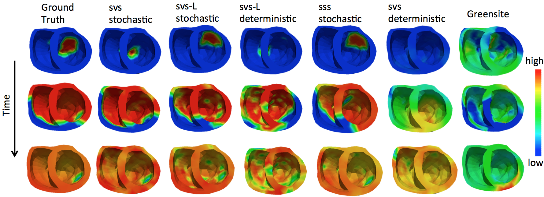
Figure 2: Comparison of TMP propagation over heart reconstructed from same ECG using different architecture. The propagation sequence is closer to ground truth in case of TMP reconstruction with svs stochastic architecture

Experiments & Results

Dataset

We simulated training and test sets using three human-torso geometry models. Spatiotemporal TMP sequences were generated using the Aliev-Panfilov (AP) model (?), and projected to the body-surface potential data with 40dB SNR noises. Two parameters were varied when simulating the TMP data : the origin of excitation and abnormal tissue properties representing myocardial scar.

The training set was randomly selected with regard to these two parameters. To test generalization ability, test data were selected with different origins of excitation and shape/location of abnormal tissues than those used in training. In particular, we prepared test datasets of four types: 1) Scar: Low, Exc: Low, 2) Scar: Low, Exc: High, 3) Scar:High, Exc: Low, and 4) Scar: High, Exc: High, where Scar/Exc indicates the parameter being varied and High/Low denotes the level of difference from the training data.

Implementation Details

For all five models being compared (svs stochastic/deterministic, svs-L stochastic/ deterministic, and sss stochastic), we used ReLU activation functions in both the encoder and decoder, ADAM optimizer (?), and a learning rate of $10^{-3}$. Each neural network was trained on approximately 2500 TMP simulations on each geometry. In addition to the five neural networks, we included a classic TMP inverse reconstruction method (Greensite) designed to incorporate temporal information (?). On each geometry, a random set of 100 test cases was selected from the test set and the process was repeated 120 times. We report the average and standard deviation of the results across all three geometry models.

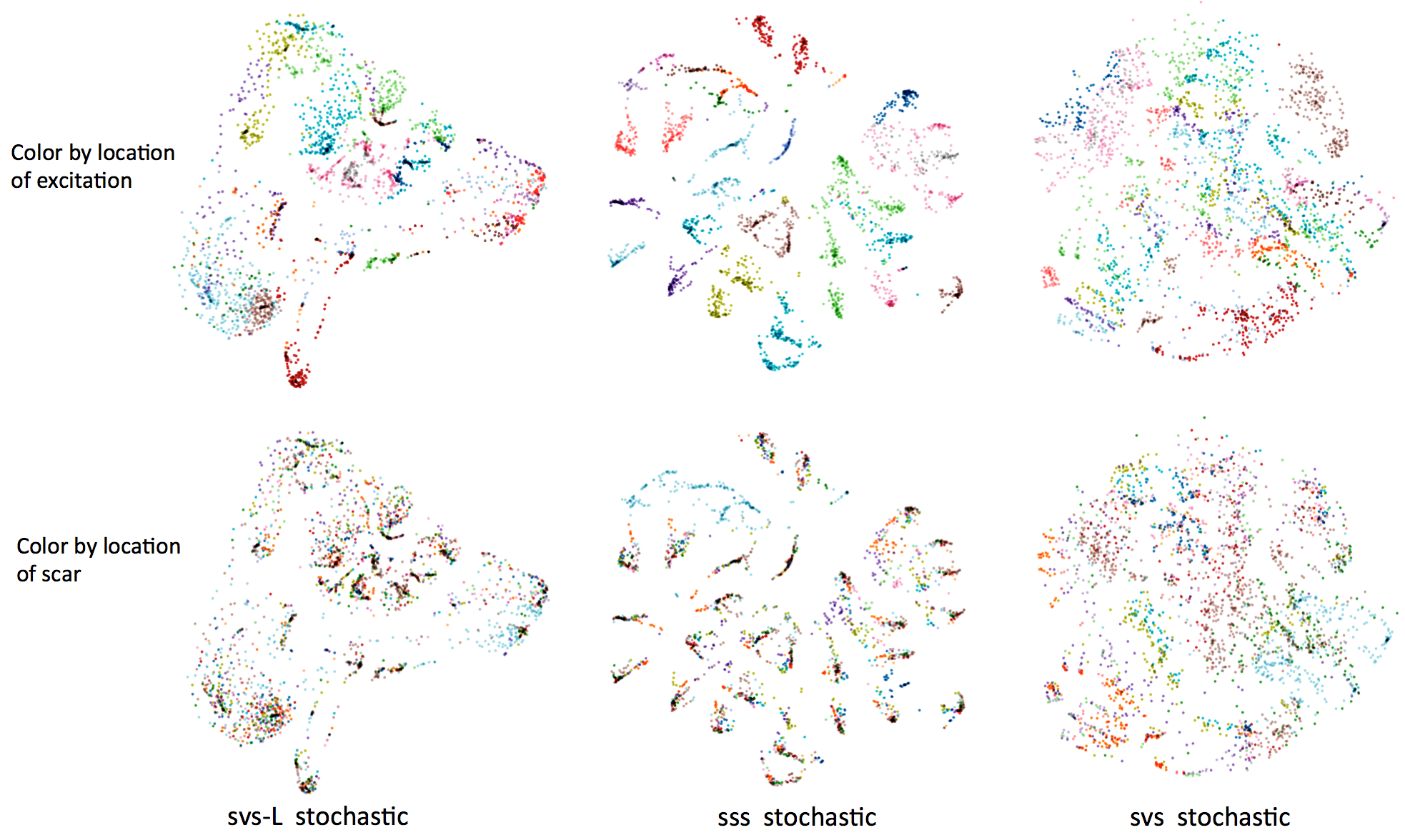
Figure 3: Visualization of latent point cloud corresponding to whole dataset: training and validation dataset.

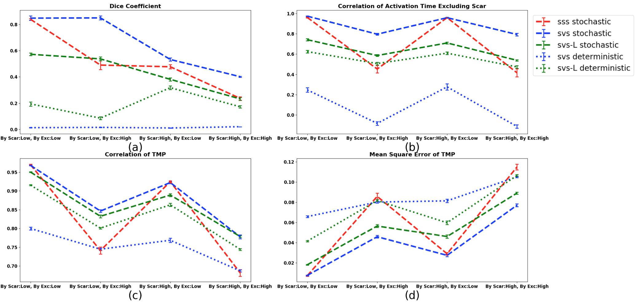
Figure 4: Comparison of reconstruction ability of different architecture at the presence of different types of unseen test data.

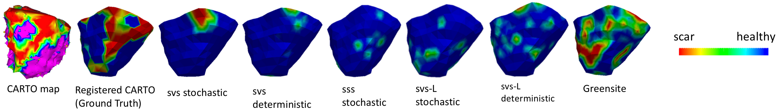
Figure 5: Comparison of scar region identified by different architectures and Greensite method with reference to in vivo CARTO map.

Results

Table 1: Metric for each method

o 0.48 — p1.7cm—— X[c] —X[c] — X[c] — X[r] — Metric	MSE	TMP Corr.	AT Corr.	Dice Coeff.
svs stochastic	$\mathbf{0.037}\pm\mathbf{0.021}$	$\mathbf{0.885}\pm\mathbf{0.061}$	$\mathbf{0.885}\pm\mathbf{0.072}$	$\mathbf{0.645}\pm\mathbf{0.181}$
svs deterministic	$0.075\pm 0.013$	$0.77\pm 0.038$	$0.12\pm 0.13$	$0.01\pm 0.006$
sss stochastic	$0.052\pm 0.035$	$0.847\pm 0.09$	$0.731\pm 0.21$	$0.531\pm 0.198$
svs-L stochastic	$0.068\pm 0.023$	$0.838\pm 0.053$	$0.601\pm 0.074$	$0.28\pm 0.154$
svs-L deterministic	$0.067\pm 0.02$	$0.84\pm 0.053$	$0.57\pm 0.052$	$0.165\pm 0.092$
Greensite	–	–	$0.514\pm 0.006$	$0.138\pm 0.005$

The reconstruction accuracy was measured with four metrics: 1) mean square error (MSE) of the TMP sequence, 2) correlation of the TMP sequence, 3) correlation of TMP-derived activation time (AT), excluding late activation due to abnormal scar tissue to focus the measure on the accuracy related to excitation points, and 4) dice coefficients of the abnormal scar tissue identified from the TMP sequence.

Table 1 summarizes the results from the three geometry models on all datasets. As shown, accuracy of the svs stochastic architecture was significantly higher than other architectures in all metrics. Similarly, the stochastic version of each architecture was more accurate than its deterministic counterpart. Most of the networks delivered a higher accuracy than the classic Greensite method (which does not preserve TMP signal shape and thus its MSE and correlation of TMP was not reported). These observations are reflected in the example of reconstructed TMP sequences in Fig. 2.

Analysis of latent representation:

To understand the difference in the latent representations obtained among different architectures, we computed latent projections of the training and validation sets for each method, and visualized the point cloud in the latent space with t-SNE (?) as shown in Fig.3. Each data point has an excitation label and scar label corresponding to their locations in the heart. The first row shows latent points colored by the excitation label, suggesting that all three stochastic models were able to cluster data points in the latent space according to the origin of excitation. The second row shows latent points colored by scar label. In this case, only the latent cloud from the svs stochastic model was clustered. This suggests that the latent representation of the presented svs stochastic model considered information of both the scar location and origin of excitation, while the other models were more focused on the excitation point.

Analysis of performance under different test conditions:

Figure 4 compares the performance of different methods in the four aforementioned types of test dataset, considering two levels of differences in each of the two parameters (excitation points and scar tissue) relative to the training data.

When only the level of unseen excitation points increases in the new data (see Fig. 4.a first two points on x axis), the dice coefficient decreased in all architectures except for the svs stochastic model. This suggests that the representation of scar location in the svs stochastic model is more robust to errors in the excitation point. On the other hand, correlation of AT shows that when only the level of unseen scar tissues varies (see Fig. 4.b first and third points on x axis), the performance of all methods stay at a constant level showing that they all encode the origin of excitation. These two findings were also consistent with the visualization of latent cloud in Fig. 3.

Comparing all the metrics, we observed that even though all the models were trained on scaled mean square loss, the stochastic models and svs stochastic performed better in identifying origin of excitation and region of scar. This suggests that stochasticity combined with aggregation of sequence information helps capture global generative factors and thus improves generalization ability.

Performance on Real Data:

We present a real-data case study on a patient who underwent catheter ablation due to scar-related ventricular tachycardia. First, the presented models were trained on data simulated on this patient as described earlier. Then, TMP was reconstructed from the real ECG data using the trained networks, from which the scar region was delineated based on TMP duration and compared with low-voltage regions from in-vivo mapping data. As shown in Fig. 5, the identified region of scar from the svs stochastic model is the closest to the in-vivo data, which is consistent with simulated results.

Conclusion

To our knowledge, this is the first work connecting VAE type of stochastic regularization with the generalization ability of a neural network. We have shown both theoretically and experimentally on inverse TMP reconstruction that the stochasticity and global aggregation of temporal information indeed improves inverse reconstruction. Future works will extend these analyses on a wider variety of image and signal reconstruction problems over time sequences.

References

- [Aliev and Panfilov 1996] Aliev, R. R., and Panfilov, A. V. 1996. A simple two-variable model of cardiac excitation. Chaos, Solitons & Fractals 7(3):293–301.
- [Bahdanau, Cho, and Bengio 2014] Bahdanau, D.; Cho, K.; and Bengio, Y. 2014. Neural machine translation by jointly learning to align and translate. arXiv preprint arXiv:1409.0473.
- [Bowman et al. 2015] Bowman, S. R.; Vilnis, L.; Vinyals, O.; Dai, A. M.; Jozefowicz, R.; and Bengio, S. 2015. Generating sentences from a continuous space. arXiv preprint arXiv:1511.06349.
- [Chen et al. 2017] Chen, H.; Zhang, Y.; Zhang, W.; Liao, P.; Li, K.; Zhou, J.; and Wang, G. 2017. Low-dose ct via convolutional neural network. Biomedical optics express 8(2):679–694.
- [Fischer et al. 2015] Fischer, P.; Dosovitskiy, A.; Ilg, E.; Häusser, P.; Hazırbaş, C.; Golkov, V.; Van der Smagt, P.; Cremers, D.; and Brox, T. 2015. Flownet: Learning optical flow with convolutional networks. arXiv preprint arXiv:1504.06852.
- [Graves 2013] Graves, A. 2013. Generating sequences with recurrent neural networks. arXiv preprint arXiv:1308.0850.
- [Greensite and Huiskamp 1998] Greensite, F., and Huiskamp, G. 1998. An improved method for estimating epicardial potentials from the body surface. IEEE TBME 45(1):98–104.
- [Hardy 1906] Hardy, G. H. 1906. On double fourier series and especially those which represent the double zeta-function with real and incommensurable parameters. Quart. J. Math 37(5).
- [Jin et al. 2017] Jin, K. H.; McCann, M. T.; Froustey, E.; and Unser, M. 2017. Deep convolutional neural network for inverse problems in imaging. IEEE Transactions on Image Processing 26(9):4509–4522.
- [Kalchbrenner and Blunsom 2013] Kalchbrenner, N., and Blunsom, P. 2013. Recurrent continuous translation models. In Proceedings of the 2013 Conference on Empirical Methods in Natural Language Processing, 1700–1709.
- [Kawaguchi and Bengio 2018] Kawaguchi, K., and Bengio, Y. 2018. Generalization in machine learning via analytical learning theory. arXiv preprint arXiv:1802.07426.
- [Kingma and Ba 2014] Kingma, D. P., and Ba, J. 2014. Adam: A method for stochastic optimization. arXiv preprint arXiv:1412.6980.
- [Kingma and Welling 2013] Kingma, D. P., and Welling, M. 2013. Auto-encoding variational bayes. arXiv preprint arXiv:1312.6114.
- [Lipton et al. 2015] Lipton, Z. C.; Kale, D. C.; Elkan, C.; and Wetzel, R. 2015. Learning to diagnose with lstm recurrent neural networks. arXiv preprint arXiv:1511.03677.
- [Lucas et al. 2018] Lucas, A.; Iliadis, M.; Molina, R.; and Katsaggelos, A. K. 2018. Using deep neural networks for inverse problems in imaging: beyond analytical methods. IEEE Signal Processing Magazine 35(1):20–36.
- [Luong, Pham, and Manning 2015] Luong, M.-T.; Pham, H.; and Manning, C. D. 2015. Effective approaches to attention-based neural machine translation. arXiv preprint arXiv:1508.04025.
- [Maaten and Hinton 2008] Maaten, L. v. d., and Hinton, G. 2008. Visualizing data using t-sne. JMLR 9(Nov):2579–2605.
- [MacLeod et al. 1995] MacLeod, R. S.; Gardner, M.; Miller, R. M.; and HORÁC̆UEK, B. M. 1995. Application of an electrocardiographic inverse solution to localize ischemia during coronary angioplasty. Journal of cardiovascular electrophysiology 6(1):2–18.
- [Mao, Shen, and Yang 2016] Mao, X.; Shen, C.; and Yang, Y.-B. 2016. Image restoration using very deep convolutional encoder-decoder networks with symmetric skip connections. In Advances in neural information processing systems, 2802–2810.
- [Pathak et al. 2016] Pathak, D.; Krahenbuhl, P.; Donahue, J.; Darrell, T.; and Efros, A. A. 2016. Context encoders: Feature learning by inpainting. In Proceedings of the IEEE Conference on Computer Vision and Pattern Recognition, 2536–2544.
- [Plonsey 1969] Plonsey, R. 1969. Bioelectric phenomena.
- [Ramanathan et al. 2004] Ramanathan, C.; Ghanem, R. N.; Jia, P.; Ryu, K.; and Rudy, Y. 2004. Noninvasive electrocardiographic imaging for cardiac electrophysiology and arrhythmia. Nature medicine 10(4):422.
- [Sutskever, Vinyals, and Le 2014] Sutskever, I.; Vinyals, O.; and Le, Q. V. 2014. Sequence to sequence learning with neural networks. In Advances in neural information processing systems, 3104–3112.
- [Wang et al. 2010] Wang, L.; Zhang, H.; Wong, K. C.; Liu, H.; and Shi, P. 2010. Physiological-model-constrained noninvasive reconstruction of volumetric myocardial transmembrane potentials. IEEE Transactions on Biomedical Engineering 57(2):296–315.
- [Wang et al. 2013] Wang, L.; Dawoud, F.; Yeung, S.-K.; Shi, P.; Wong, K. L.; Liu, H.; and Lardo, A. C. 2013. Transmural imaging of ventricular action potentials and post-infarction scars in swine hearts. IEEE TMI 32(4):731–747.
- [Wang et al. 2015] Wang, Z.; Liu, D.; Yang, J.; Han, W.; and Huang, T. 2015. Deep networks for image super-resolution with sparse prior. In Proceedings of the IEEE International Conference on Computer Vision, 370–378.
- [Wang et al. 2016] Wang, S.; Su, Z.; Ying, L.; Peng, X.; Zhu, S.; Liang, F.; Feng, D.; and Liang, D. 2016. Accelerating magnetic resonance imaging via deep learning. In Biomedical Imaging (ISBI), 2016 IEEE 13th International Symposium on, 514–517. IEEE.
- [Wang et al. 2018] Wang, L.; Gharbia, O. A.; Horacek, B. M.; Nazarian, S.; ; and Sapp, J. L. 2018. Noninvasive epicardial and endocardial electrocardiographic imaging of scar-related ventricular tachycardia. EP Europace under review after major revision.
- [Werbos 1990] Werbos, P. J. 1990. Backpropagation through time: what it does and how to do it. Proceedings of the IEEE 78(10):1550–1560.
- [Yao et al. 2017] Yao, H.; Dai, F.; Zhang, D.; Ma, Y.; Zhang, S.; Zhang, Y.; and Tian, Q. 2017. Dr2-net: Deep residual reconstruction network for image compressive sensing. arXiv preprint arXiv:1702.05743.
- [Yue-Hei Ng et al. 2015] Yue-Hei Ng, J.; Hausknecht, M.; Vijayanarasimhan, S.; Vinyals, O.; Monga, R.; and Toderici, G. 2015. Beyond short snippets: Deep networks for video classification. In Proceedings of the IEEE conference on computer vision and pattern recognition, 4694–4702.
- [Zhu et al. 2018] Zhu, B.; Liu, J. Z.; Cauley, S. F.; Rosen, B. R.; and Rosen, M. S. 2018. Image reconstruction by domain-transform manifold learning. Nature 555(7697):487.