Tilt Rotations and the Tilt Phase Space

Abstract

In this paper, the intuitive idea of tilt is formalised into the rigorous concept of tilt rotations. This is motivated by the high relevance that pure tilt rotations have in the analysis of balancing bodies in 3D, and their applicability to the analysis of certain types of contacts. The notion of a ‘tilt rotation’ is first precisely defined, before multiple parameterisations thereof are presented for mathematical analysis. It is demonstrated how such rotations can be represented in the so-called tilt phase space, which as a vector space allows for a meaningful definition of commutative addition. The properties of both tilt rotations and the tilt phase space are also extensively explored, including in the areas of spherical linear interpolation, rotational velocities, rotation composition and rotation decomposition.

I Introduction

Tilt rotations first arose in the context of the fused angles and tilt angles rotation representations, as a way of partitioning 3D rotations into independent yaw and tilt components [1]. They are highly relevant for situations like the analysis of balancing bodies in 3D—e.g. bipedal robots [2] [3], as the yaw component does not contribute to the body-local state of balance—but can also be used for other purposes. For example, tilt rotations can be used to represent the relative orientations of contacting bodies, or the relative rotations of two planar surfaces, such as for instance the foot of a robot and the ground. This paper seeks to comprehensively investigate tilt rotations, the parameterisations and properties they have, and their possible algorithmic applications. As part of this, the novel tilt phase space representation is introduced, which amongst other things allows for tilt rotations to be commutatively combined in a way akin to addition. Complete definitions of tilt rotations and the tilt phase space can be found in Section IV–V, but as an illustrative guide, Fig. 1 shows three different tilt rotations applied to a robot, along with the corresponding axes of rotation. For tilt rotations, by definition the axis of rotation must lie in the horizontal $\mathbf{xy}$ plane, as shown, and plotting the magnitude of the rotation at the polar angle corresponding to the axis of rotation gives the three 2D tilt phase space points shown on the right hand side in Fig. 1. When combined with a yaw component, e.g. to form the 3D tilt phase space, tilt rotations can be used to quantify and analyse any general 3D rotation.

In addition to the formalisation of the idea of referenced rotations (see Section III-B), the main contributions of this paper lie in the systematisation of the concept of tilt rotations, the introduction of the novel tilt phase space, and the investigation of the many properties and results of both. Open source software libraries in C++ and Matlab have also been released to explicitly support tilt rotations, and computations and conversions involving the tilt phase space.

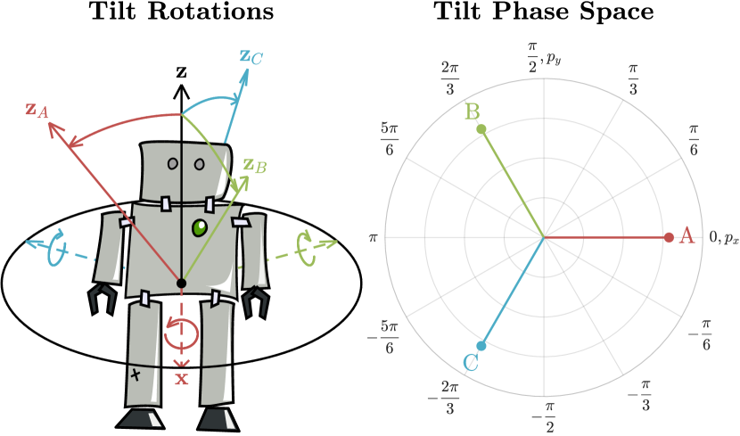
Figure 1: Diagram showing three different example tilt rotations A, B and C (left), and the corresponding points in the tilt phase space (right). More details on the definitions of both concepts follow in Section IV–V.

II Related Work

Tilt rotations have been used in previous works, for example for the modelling of heading-independent balance states while walking [3], and for the modelling of foot orientations and ground contacts [4]. The tilt phase space has also been used as the fundamental basis for an entire bipedal walking feedback controller [2], which was possible only due to its unique set of properties. Tilt rotations were first formulated as part of the definition of fused angles and tilt angles, but were not significantly further investigated in their own right. These two representations, in addition to the tilt phase space representation presented here, were developed to provide a robust and geometrically intuitive way of quantifying the components of rotation of a body in each of the three major planes, namely the $\mathbf{xy}$, $\mathbf{yz}$ and $\mathbf{xz}$ planes [1]. This is something that quaternions and Euler angles do not do, as discussed in extensive detail in [5]. As a result, any attempt to define the concept of a ‘tilt rotation’ for example as the combination of Euler pitch and roll, would be mathematically unhelpful, and not correspond to human intuition of ‘tilt’. A thorough review of all kinds of rotation representations, such as for example quaternions, rotation matrices, axis-angle pairs [6] and vectorial parameterisations [7] [8], can be found in [1]. The representation most closely related to the tilt phase space is the rotation vector [9]. Two of the tilt phase parameters can be expressed as the rotation vector parameters of the tilt rotation component (see Section IV-A) of a rotation. There is no correspondence to the rotation vector parameters of the full rotation however.

III Preliminaries

This section introduces the notation and basic identities that are used throughout the remainder of this paper.

III-A Notation and Conventions

As is standard for the analysis of fused angles and tilt angles, we use the convention that the z-axis points ‘up’, where this is generally defined to be in the opposite direction to gravity, or along a particular surface normal, as required. The global fixed frame is taken to be {G}, and the body-fixed frame of interest is taken to be {B}. The rotation $\tensor*[^{G}_{B}]{R}{}$ refers to the rotation from {G} to {B}, namely

$$\tensor*[^{G}_{B}]{R}{}=\begin{bmatrix}\tensor*[^{G}]{\mathbf{x}}{{}_{B}}&\tensor*[^{G}]{\mathbf{y}}{{}_{B}}&\tensor*[^{G}]{\mathbf{z}}{{}_{B}}\end{bmatrix}=\begin{bmatrix}\tensor*[^{B}]{\mathbf{x}}{{}_{G}}&\tensor*[^{B}]{\mathbf{y}}{{}_{G}}&\tensor*[^{B}]{\mathbf{z}}{{}_{G}}\end{bmatrix}^{T}\!\!,$$ (1)

where for example $\tensor*[^{G}]{\mathbf{z}}{{}_{B}}$ is the unit vector corresponding to the positive z-axis of {B}, expressed in the coordinates of {G}. We further follow the convention that, for example,

$$\tensor*[^{G}]{\mathbf{z}}{{}_{B}}=\bigl{(}\tensor*[^{G}]{z}{{}_{Bx}},\tensor*[^{G}]{z}{{}_{By}},\tensor*[^{G}]{z}{{}_{Bz}}\bigr{)}.$$ (2)

If the superscript basis frame is omitted, e.g. like in ‘$\tensor*{\mathbf{z}}{{}_{B}}$’, by default it is the global fixed frame {G}.

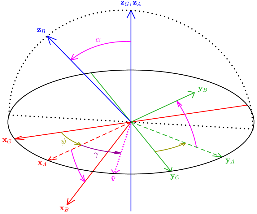
Figure 2: Diagram of the tilt angles parameters $(\psi,\gamma,\alpha)$. A z-rotation by $\psi$ from {G} to {A} is followed by a rotation by $\alpha$ about $\mathbf{\hat{v}}$ from {A} to {B}.

III-B Referenced Rotations

Given frames {A} and {B} relative to a global frame {G}, the global rotation that maps {A} onto {B} is given by

$$\tensor*[^{GA}_{B}]{R}{}=\tensor*[^{G}_{B}]{R}{}\,\tensor*[^{A}_{G}]{R}{},$$ (3)

where $\tensor*[^{GA}_{B}]{R}{}$ is new notation for the rotation from frame {A} to {B} referenced by {G}. Alternative mathematical formulations for this so-called referenced rotation include

$$\tensor*[^{GA}_{B}]{R}{}=\tensor*[^{G}_{A}]{R}{}\,\tensor*[^{A}_{B}]{R}{}\,\tensor*[^{G}_{A}]{R}{}^{T}\!=\tensor*[^{G}_{B}]{R}{}\,\tensor*[^{A}_{B}]{R}{}\,\tensor*[^{G}_{B}]{R}{}^{T}\!.$$ (4)

It should be noted that referenced rotations are just a direct generalisation of standard rotations, as from (3) we have

$$\tensor*[^{G}_{B}]{R}{} \equiv\tensor*[^{GG}_{B}]{R}{}, \tensor*[^{A}_{G}]{R}{} \equiv\tensor*[^{GA}_{G}]{R}{}, \tensor*[^{GA}_{A}]{R}{} =\mathbb{I}.$$ (5)

Basic identities involving referenced rotations include

$$\tensor*[^{GA}_{B}]{R}{}\,\tensor*[^{G}_{A}]{R}{} =\tensor*[^{G}_{B}]{R}{}, \tensor*[^{G}_{A}]{R}{}^{T}\!\,\tensor*[^{GA}_{B}]{R}{}\,\tensor*[^{G}_{A}]{R}{} =\tensor*[^{A}_{B}]{R}{},$$ (6)

$$\tensor*[^{B}_{G}]{R}{}\,\tensor*[^{GA}_{B}]{R}{} =\tensor*[^{A}_{G}]{R}{}, \tensor*[^{G}_{B}]{R}{}^{T}\!\,\tensor*[^{GA}_{B}]{R}{}\,\tensor*[^{G}_{B}]{R}{} =\tensor*[^{A}_{B}]{R}{}.$$ (7)

Composition and inversion is given by

$$\tensor*[^{GA}_{C}]{R}{} =\tensor*[^{GB}_{C}]{R}{}\,\tensor*[^{GA}_{B}]{R}{}, \tensor*[^{GA}_{B}]{R}{}^{T}\! =\tensor*[^{GB}_{A}]{R}{}.$$ (8)

Finally, a change of referenced frame is given by

$$\tensor*[^{HA}_{B}]{R}{}=\tensor*[^{H}_{G}]{R}{}\,\tensor*[^{GA}_{B}]{R}{}\,\tensor*[^{H}_{G}]{R}{}^{T}\!.$$ (9)

Referenced rotations are required for Section VI-G.

IV Definition of Tilt Rotations

In the fused angles and tilt angles representations, the yaw component of rotation is quantified using the fused yaw [1], defined below in Section IV-A. Tilt rotations are exactly the rotations that have a zero fused yaw component. As such, all rotations can be neatly partitioned into their fused yaw and tilt rotation components, as described later in Section VI-E. Tilt rotations can however also be characterised as precisely the rotations that can be expressed as a pure rotation about a vector in the $\mathbf{xy}$ plane. The following sections detail the various available parameterisations of tilt rotations.

IV-A Definition of Fused Yaw

Given a rotation from {G} to {B}, as illustrated in Fig. 2, we define a frame {A} by rotating {B} in such a way that $\tensor*{\mathbf{z}}{{}_{B}}$ rotates onto $\tensor*{\mathbf{z}}{{}_{G}}$ in the most direct way possible, within the plane that contains these two vectors. Note that this rotation of {B} is in the opposite direction to the arrow labelled ‘$\alpha$’ in the figure. The fused yaw $\psi\in(-\pi,\pi]$ is then given by the angle of the pure z-rotation from {G} to {A}. The remaining rotation from {A} to {B} is a tilt rotation, and is referred to as the tilt rotation component of the total rotation. If $\tensor*[^{G}_{B}]{q}{}=(w,x,y,z)\in\mathbb{Q}$ is the quaternion rotation from {G} to {B}, then mathematically the fused yaw is given by

$$\psi=\operatorname{wrap}\bigl{(}2\operatorname{atan2}(z,w)\bigr{)},$$ (10)

where $\operatorname{wrap}(\cdot)$ is a function that wraps an angle to $(-\pi,\pi]$. The fused yaw has an essential discontinuity at $w=z=0$, which is simply referred to as the fused yaw singularity.

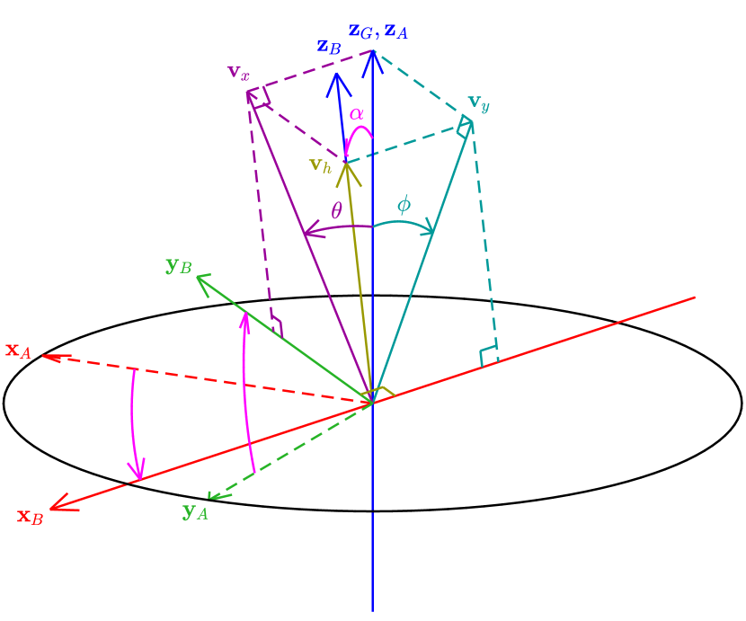
Figure 3: Diagram of the fused angles parameters $(\theta,\phi,h)$. The rotation by $\alpha$ from {A} to {B} is reparameterised by the angles $\theta$ and $\phi$, defined between $\tensor*{\mathbf{z}}{{}_{G}}$ and the $\tensor*{\mathbf{y}}{{}_{B}}\tensor*{\mathbf{z}}{{}_{B}}$ and $\tensor*{\mathbf{x}}{{}_{B}}\tensor*{\mathbf{z}}{{}_{B}}$ planes respectively. The hemisphere $h$ is $1$ if $\tensor*{\mathbf{v}}{{}_{h}}$ is parallel to $\tensor*{\mathbf{z}}{{}_{B}}$, and $-1$ if it is antiparallel.

IV-B Parameterisations of Tilt Rotations

IV-B1 Tilt Angles Parameterisation

The tilt rotation component, i.e. the rotation from {A} to {B}, can be parameterised by the two parameters $(\gamma,\alpha)$. The tilt angle $\alpha$ is the magnitude of the rotation, and the tilt axis angle $\gamma$ defines the tilt axis $\mathbf{\hat{v}}$ in the $\tensor*{\mathbf{x}}{{}_{G}}\tensor*{\mathbf{y}}{{}_{G}}$ plane about which the rotation occurs, as shown in Fig. 2. Together with the fused yaw $\psi$, these two parameters define the tilt angles representation

$$\tensor*[^{G\mspace{2.0mu}}_{B}]{T}{}=(\psi,\gamma,\alpha)\in(-\pi,\pi]{\times}(-\pi,\pi]{\times}[0,\pi]\equiv\mathbb{T}.$$ (11)

If $\tensor*[^{G}_{B}]{R}{}\in\text{SO}(3)$ is the rotation matrix for the rotation from {G} to {B}, and $R_{ij}$ are the corresponding rotation matrix entries, then mathematically, $\gamma$ and $\alpha$ are given by

$$\gamma =\operatorname{atan2}(-R_{31},R_{32}), \alpha =\operatorname{acos}(R_{33}).$$ (12)

By extending the domain of $\alpha$ to $[0,\infty)$, tilt rotations of arbitrary magnitude can be parameterised. This allows the magnitude of rotations greater than half a revolution to be captured, instead of just regarding the final resulting coordinate frame as a plain orientation.

IV-B2 Fused Angles Parameterisation

The tilt rotation component from {A} to {B} can also be parameterised using the three parameters $(\theta,\phi,h)$. The fused pitch $\theta$ and fused roll $\phi$ are defined as the signed angles between $\tensor*{\mathbf{z}}{{}_{G}}$ and the $\tensor*{\mathbf{y}}{{}_{B}}\tensor*{\mathbf{z}}{{}_{B}}$ and $\tensor*{\mathbf{x}}{{}_{B}}\tensor*{\mathbf{z}}{{}_{B}}$ planes respectively, as shown in Fig. 3. The hemisphere $h\in\{-1,1\}$ is a binary parameter specifying whether $\tensor*{\mathbf{z}}{{}_{G}}$ and $\tensor*{\mathbf{z}}{{}_{B}}$ are in the same hemisphere or not. The complete fused angles representation is then given by

$$\mspace{-8.0mu}\tensor*[^{G\mspace{1.0mu}}_{B}]{\mspace{-2.0mu}F}{}\mspace{-5.0mu}=\mspace{-4.0mu}(\psi,\theta,\phi,h)\mspace{-4.0mu}\in\mspace{-4.0mu}(\!-\pi,\pi]{\times}[\mspace{-1.0mu}-\tfrac{\pi}{2},\tfrac{\pi}{2}]{\times}[\mspace{-1.0mu}-\tfrac{\pi}{2},\tfrac{\pi}{2}]{\times}\{\!-1,1\}\mspace{-1.0mu}.\mspace{-3.0mu}$$ (13)

Mathematically, the fused angles parameters are given by

$$\mspace{-6.0mu}\theta =\operatorname{asin}(-R_{31}), \phi =\operatorname{asin}(R_{32}), h =\operatorname{sign}(R_{33}).$$ (14)

The relationship between $(\theta,\phi)$ and $(\gamma,\alpha)$ is given by

$$\theta =\operatorname{asin}(\sin\alpha\sin\gamma), \phi =\operatorname{asin}(\sin\alpha\cos\gamma).$$ (15)

IV-B3 Z-Vector Parameterisation

Recalling (1), it can be seen from (12) and (14) that tilt rotations are a unique function of the corresponding z-vector $\tensor*[^{B}]{\mathbf{z}}{{}_{G}}$—at least away from the fused yaw singularity. In fact,

$$\tensor*[^{B}]{\mathbf{z}}{{}_{G}} =\bigl{(}-\sin\alpha\sin\gamma,\,\sin\alpha\cos\gamma,\,\cos\alpha\bigr{)}$$ (16)

$$=\Bigl{(}-\sin\theta,\,\sin\phi,\,h\sqrt{1-\sin^{2}\theta-\sin^{2}\phi}\,\Bigr{)}\mspace{-2.0mu}.$$ (17)

IV-B4 Quaternion Parameterisation

A rotation is a tilt rotation if and only if the z-component of the corresponding quaternion is zero. As such, a tilt rotation can be parameterised by its quaternion parameters

$$\mspace{-6.0mu}q=(w,x,y,0)=(\cos\tfrac{\alpha}{2},\,\sin\tfrac{\alpha}{2}\cos\gamma,\,\sin\tfrac{\alpha}{2}\sin\gamma,\,0).$$ (18)

V Definition of the Tilt Phase Space

When working with tilt rotations and how to combine them, the tilt angles parameterisation is frequently the representation of choice. In addition to providing an intuitive notion of the direction of tilt, which is helpful in many applications, the tilt angle parameter can also be extended to the domain $\alpha\in[0,\infty)$, allowing tilt rotations of unbounded magnitude to be represented and used for analysis. Rotation composition as a method of combining tilt rotations is unsuitable however, as the composition of tilt rotations is not closed, not commutative, and invariantly returns a bounded $\alpha$ for the rotation output. This shortcoming is one of the features that is addressed by the tilt phase space.

The tilt angles parameterisation also has the problem that it has a discontinuity in the tilt axis angle $\gamma$ at the identity rotation, and that the tilt angle $\alpha$ is not differentiable there due to a cusp [1]. This leads to numerical and algorithmic difficulties, in particular if attempting to express tilt angles velocities, and attempting to relate them to angular velocities. This problem is similarly addressed by the tilt phase space.

There are two main variations of the tilt phase space, relative and absolute, and for each there is a choice of 2D or 3D, depending on whether the fused yaw is included or not. All four of these spaces are entirely analogous, however, so we can speak of just ‘the’ tilt phase space.

V-A Relative Tilt Phase Space

This is the default variant of the tilt phase space. By convention, the qualifier ‘relative’ is only ever used if it is required to explicitly differentiate between the relative and absolute variants. Given the tilt angles representation $T=(\psi,\gamma,\alpha)$ of a rotation, the equivalent 3D tilt phase space representation is given by

$$P=(p_{x},p_{y},p_{z})=(\alpha\cos\gamma,\,\alpha\sin\gamma,\,\psi)\in\mathbb{R}^{3}\equiv\mathbb{P}^{3}.$$ (19)

Often when working with tilt rotations, the fused yaw component is not required. In such cases, the 2D tilt phase space representation can be used instead, given by

$$P=(p_{x},p_{y})=(\alpha\cos\gamma,\,\alpha\sin\gamma)\in\mathbb{R}^{2}\equiv\mathbb{P}^{2}.$$ (20)

This is the predominant formulation of the tilt phase space that is used in analysis. Note that in (19–20), a domain of $\mathbb{R}$ has been specified for the parameters, to naturally be able to represent rotations of more than 180^∘. The conversion from the relative tilt phase space to tilt angles is given by

$$\psi =p_{z}, \gamma =\operatorname{atan2}(p_{y},p_{x}), \alpha =\sqrt{p_{x}^{2}+p_{y}^{2}}\mspace{2.0mu}.$$ (21)

The relationship between the 2D tilt phase parameters and the tilt angles parameters is shown visually in Fig. 4. The 2D tilt phase is to the tilt angles $(\gamma,\alpha)$ for tilt rotations, what cartesian coordinates is to polar coordinates for points.

It should be noted that the tilt phase parameters are globally continuous and smooth functions of the underlying rotation, in the sense that they are infinitely differentiable. This is a critically important property, and it is not trivial to see why this holds at $p_{x}=p_{y}=0$, but it provably does. As such, differentiated quantities, such as for example tilt phase velocities and accelerations, are well-defined everywhere and can be smoothly converted to other representations, such as for example angular velocities and angular accelerations.

V-B Absolute Tilt Phase Space

The absolute tilt phase space shares the same definition as the relative tilt phase space, only with the absolute tilt axis angle ${\tilde{\gamma}}={\gamma+\psi}$ being used instead of $\gamma$. That is,

$$\tilde{P} =(\tilde{p}_{x},\tilde{p}_{y},\tilde{p}_{z}) =(\alpha\cos{\tilde{\gamma}},\,\alpha\sin{\tilde{\gamma}},\,\psi) \in\mathbb{R}^{3}\equiv\tilde{\mathbb{P}}^{3},$$ (22)

$$\tilde{P} =(\tilde{p}_{x},\tilde{p}_{y}) =(\alpha\cos{\tilde{\gamma}},\,\alpha\sin{\tilde{\gamma}}) \in\mathbb{R}^{2}\equiv\tilde{\mathbb{P}}^{2}.$$ (23)

The conversions to the relative space and back are given by

$$p_{x} = c_{\psi}\tilde{p}_{x}+s_{\psi}\tilde{p}_{y}, \tilde{p}_{x} =c_{\psi}p_{x}-s_{\psi}p_{y},$$ (24)

$$p_{y} =- s_{\psi}\tilde{p}_{x}+c_{\psi}\tilde{p}_{y}, \tilde{p}_{y} =s_{\psi}p_{x}+c_{\psi}p_{y},$$

where $c_{\ast}\equiv\cos\ast$ and $s_{\ast}\equiv\sin\ast$. As the two spaces are so tightly linked, all of the results that hold for one space correspond trivially to analogous results for the other. The two spaces are also negative inverses of one another, i.e.

$$P^{-1} =-\tilde{P}, \tilde{P}^{-1} =-P.$$ (25)

As $\tilde{P}\equiv P$ for pure tilt rotations, as a corollary

$$p_{z}=0\mspace{12.0mu}\implies\mspace{10.0mu}P^{-1}=-P.$$ (26)

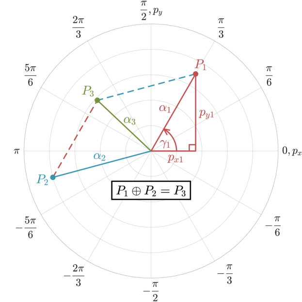
Figure 4: Tilt phase plot demonstrating tilt vector addition (see Section V-D), and the link between the tilt phase and tilt angles parameters.

V-C Fundamental Properties of the Tilt Phase Space

Similar to fused angles, the tilt phase space has numerous properties [5] that set it apart from alternatives such as for example Euler angles. The parameters are mutually independent and correspond to different major planes of rotation, the yaw, i.e. $p_{z}$, is axisymmetric, and the two remaining tilt parameters are axisymmetric and correspond to each other in behaviour. A unique property of the tilt phase space however, is magnitude axisymmetry. This relates to the fact that equal angle magnitude rotations in any tilt direction have equal norms in the 2D tilt phase space. This is not the case for the pitch and roll components of fused angles.

V-D Tilt Vector Addition

Although the composition of tilt rotations is not commutative and in general does not produce a tilt rotation as an output, the 2D tilt phase space provides a way of defining a useful and meaningful addition operator for tilt rotations that is closed, commutative and associative. This is referred to as tilt vector addition, and for $P_{1},P_{2}\in\mathbb{P}^{2}$ is given by

$$\begin{split}P_{3}=P_{1}\oplus P_{2}&=(p_{x1}+p_{x2},\,p_{y1}+p_{y2})\in\mathbb{P}^{2}\\ &=(\alpha_{1}c_{\gamma_{1}}+\alpha_{2}c_{\gamma_{2}},\,\alpha_{1}s_{\gamma_{1}}+\alpha_{2}s_{\gamma_{2}}).\end{split}$$ (27)

(21) can be used to calculate the tilt angles parameters $(\gamma_{3},\alpha_{3})$ corresponding to $P_{3}$. In abbreviated form, we write

$$(\gamma_{1},\alpha_{1})\oplus(\gamma_{2},\alpha_{2})=(\gamma_{3},\alpha_{3}).$$ (28)

The action of tilt vector addition is illustrated in Fig. 4. Completely analogous definitions of tilt vector addition hold for the absolute tilt phase space, where it should be noted that the addition of absolute phases is consistent with the addition of relative phases, as long as it is being done for a fixed fused yaw. In other words, if any two tilt rotations $(\gamma,\alpha)$ are converted to both relative and absolute tilt phases, and added in each representation, then the outputs expressed as, for example, quaternions are identical.

V-E Vector Space of Tilt Rotations

Based on (27), it is easy to see that $(\mathbb{P}^{2},\oplus)$ is an abelian group. For $\lambda\in\mathbb{R}$, we define scalar multiplication as

$$\lambda P=(\lambda p_{x},\lambda p_{y}).$$ (29)

This completes $\mathbb{P}^{2}$ as a vector space over $\mathbb{R}$ that is isomorphic to $\mathbb{R}^{2}$, as suggestively written in (20). This is referred to as the vector space of tilt rotations. The vector space of absolute tilt rotations is similarly defined. It is easy to verify that the additive inverses in these vector spaces in fact correspond to the true inverses of the corresponding tilt rotations. The identity vector, i.e. the zero vector, also corresponds to the true identity tilt rotation.

Given that tilt rotations can be formulated as a vector space, many useful properties, results, concepts and algorithms come for ‘free’. For instance, combining tilt vector addition with scalar multiplication leads to a trivial definition of the mean of a set of tilt rotations. Other useful corollaries of having a vector space, that are however outside of the scope of this paper, include results involving differentiation, integration, metrics and general linear algebra.

Having a vector space of tilt rotations also allows cubic spline interpolation to be performed, with the guarantee that all produced intermediate rotations are indeed tilt rotations. Other methods of orientation spline interpolation—involving for example the logarithmic and exponential map and working with the Lie algebra $\mathfrak{so}(3)$—in general do not have this required property, are significantly more computationally expensive, and cannot deal with rotations above 180^∘, albeit for the benefit of often being bi-invariant [10]. In the inherently asymmetrical situation where there is a clear notion of ‘up’, however, bi-invariance is not seen as a decisive advantage, especially when observing that tilt phase space cubic spline interpolation is in fact invariant about the ‘up’ z-axis. It should be noted that the optimal minimum angular acceleration interpolating curve between orientations is an involved three-dimensional, fourth-order nonlinear two-point boundary value problem, does not in general admit a closed form solution [10], and is thus frequently not an option.

VI Properties of Tilt Rotations and
the Tilt Phase Space

In this section, various results pertaining to tilt rotations and the tilt phase space are explored and presented.

VI-A Spherical Linear Interpolation Between Tilt Rotations

Spherical linear interpolation (slerp) is a way of interpolating rotations that is torque-minimal and constant angular velocity. Given $q_{0},q_{1}\in\mathbb{Q}$ and $u\in[0,1]$, slerp is given by

$$\operatorname{slerp}(q_{0},q_{1},u)=\left[\frac{\sin((1-u)\Omega)}{\sin{\Omega}}\right]\!q_{0}+\left[\frac{\sin u\Omega}{\sin{\Omega}}\right]\!q_{1},$$ (30)

where $\Omega=\operatorname{acos}(q_{0}\mathchoice{\mathbin{\vbox{\hbox{\scalebox{0.5}{$\displaystyle\bullet$}}}}}{\mathbin{\vbox{\hbox{\scalebox{0.5}{$\textstyle\bullet$}}}}}{\mathbin{\vbox{\hbox{\scalebox{0.5}{$\scriptstyle\bullet$}}}}}{\mathbin{\vbox{\hbox{\scalebox{0.5}{$\scriptscriptstyle\bullet$}}}}}q_{1})$, and $q_{0}$, $q_{1}$ need to be mutually in the same 4D hemisphere. It can be demonstrated that slerp between any two tilt rotations always produces a tilt rotation—a property that is less trivial than it may seem. As such, tilt rotations can always cleanly and easily be interpolated, without affecting the fused yaw. Furthermore, for any $\hat{q}\in\mathbb{Q}$,

$$\operatorname{slerp}(\hat{q}q_{0},\hat{q}q_{1},u)=\hat{q}\operatorname{slerp}(q_{0},q_{1},u).$$ (31)

Thus, by choosing $\hat{q}=q_{z}(\psi)$, i.e. the quaternion corresponding to a z-rotation by $\psi$, it follows that slerp between any two rotations of equal fused yaw always produces an output rotation of exactly the same fused yaw. That is,

$$\Psi\bigl{(}q_{0}\bigr{)}=\Psi\bigl{(}q_{1}\bigr{)}=\psi\implies\Psi\bigl{(}\operatorname{slerp}(q_{0},q_{1},u)\bigr{)}=\psi,$$ (32)

where the function $\Psi(\cdot)$ returns the fused yaw of a rotation.

VI-B Relation Between Fused Angles and the Tilt Phase Space

Just like the fused roll $\phi$ and fused pitch $\theta$ can be seen to quantify the amount of tilt rotation about the x and y-axes respectively, the tilt phase space parameters $(p_{x},p_{y})$ also do exactly that. From (21), a tilt rotation of pure $p_{x}$ corresponds by definition to a $\gamma$ of 0 or $\pi$, and hence corresponds to a pure x-rotation, as the tilt axis $\mathbf{\hat{v}}$ (see Fig. 2) is then parallel or antiparallel to the x-axis. Similarly, a tilt rotation of pure $p_{y}$ corresponds to a $\gamma$ of $\pm\tfrac{\pi}{2}$, and hence corresponds to a pure y-rotation. Furthermore, from (15),

$$\sin\phi =\sin\alpha\cos\gamma, \sin\theta =\sin\alpha\sin\gamma.$$ (33)

Applying the small angle approximation to $\phi$, $\theta$ and $\alpha$ yields

$$\phi \approx\alpha\cos\gamma=p_{x}, \theta \approx\alpha\sin\gamma=p_{y}.$$ (34)

In fact, $p_{x}$ and $p_{y}$ are from a mathematical perspective the $\mathcal{O}(\alpha^{3})$ Taylor series approximations of $\phi$ and $\theta$, respectively. As such, the 2D tilt phase parameters mimic fused angles for tilt rotations of small magnitudes, but increase linearly to infinity for large magnitudes. This is unlike $\phi$ and $\theta$, which loop around to correctly represent the resulting orientation. For example, $(\gamma,\pi)$ and $(\gamma,-\pi)$ both correspond to the same orientation in terms of fused angles, but are completely different tilt phase rotations. Put concisely, the tilt phase space is for unbounded tilt rotations, i.e. tilt rotations of more than 180^∘, what fused angles is for bounded tilt rotations—a way of concurrently quantifying in an axisymmetric manner the amount of rotation about each of the coordinate axes.

The relative differences between the fused angles and tilt phase space parameters are plotted in Fig. 5 as a function of $p_{x}$ and $p_{y}$. The plotted values are expressed as ratios of the tilt rotation magnitude $\alpha$. It can be observed that the errors in the approximations $p_{x}\approx\phi$ and $p_{y}\approx\theta$ are in fact notably less than the error involved in assuming $\sin\alpha\approx\alpha$, showing how close the parameters are for even medium rotations.

VI-C Interpretation of Tilt Vector Addition

The definition used for tilt vector addition is in part motivated by the unambiguous commutative way in which angular velocities, unlike angular rotations, can be added. The interpretation thereof as the addition of instantaneous angular velocities extends naturally to unbounded tilt rotations, as angular velocities can also have arbitrary magnitude, and do not ‘wrap around’ like rotations do. Suppose we wish to add two tilt rotations $(\gamma_{1},\alpha_{1})$ and $(\gamma_{2},\alpha_{2})$, as in (28). The tilt rotation given by $(\gamma_{1},\alpha_{1})$ is equivalent to applying an angular velocity of $\tensor*[^{G}]{\mathbf{\Omega}}{{}_{1}}$ for $t$ seconds, where

$$\tensor*[^{G}]{\mathbf{\Omega}}{{}_{1}}=\tfrac{1}{t}(\alpha_{1}c_{\gamma_{1}},\,\alpha_{1}s_{\gamma_{1}},\,0).$$ (35)

Similarly, $(\gamma_{2},\alpha_{2})$ is equivalent to $t$ seconds of

$$\tensor*[^{G}]{\mathbf{\Omega}}{{}_{2}}=\tfrac{1}{t}(\alpha_{2}c_{\gamma_{2}},\,\alpha_{2}s_{\gamma_{2}},\,0).$$ (36)

Thus, if both angular velocities are applied at the same time, the resulting total angular velocity is given by $\tensor*[^{G}]{\mathbf{\Omega}}{{}_{3}}$, where

$$\begin{split}\tensor*[^{G}]{\mathbf{\Omega}}{{}_{3}}&=\tensor*[^{G}]{\mathbf{\Omega}}{{}_{1}}+\tensor*[^{G}]{\mathbf{\Omega}}{{}_{2}}\\ &=\tfrac{1}{t}(\alpha_{1}c_{\gamma_{1}}+\alpha_{2}c_{\gamma_{2}},\,\alpha_{1}s_{\gamma_{1}}+\alpha_{2}s_{\gamma_{2}},\,0).\end{split}$$ (37)

Given that $\tensor*[^{G}]{\mathbf{\Omega}}{{}_{3}}$ is then applied for $t$ seconds, the parallel to the definition (27) of tilt vector addition is clear.

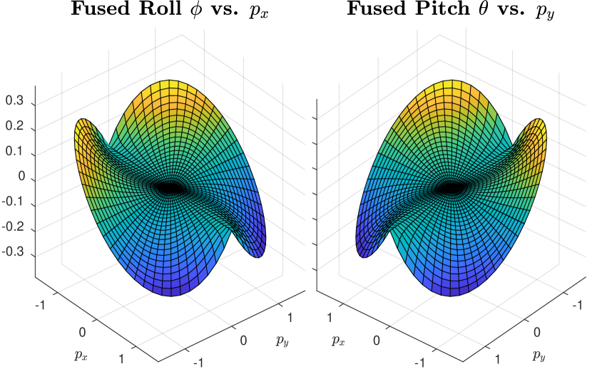
Figure 5: Plots of the relative difference, as a ratio of the tilt rotation magnitude $\alpha$, between the fused angles and tilt phase space parameters. For $\alpha=1\approx 57.3^{\circ}$, the maximum relative difference is just 7.1%, compared to 15.9% for the equivalent small angle approximation $\sin\alpha\approx\alpha$. For $\alpha=\tfrac{\pi}{2}=90^{\circ}$, these numbers are 21.1% and 36.3%, respectively.

VI-D Rotational Velocities

When working with trajectories in either the 2D tilt rotation space or the full 3D rotation space, like for example for cubic spline interpolation, it is necessary to be able to relate rotational velocities between the various representations. In particular, the relationships between the tilt phase velocities $\dot{P}=\bigl{(}\dot{p}_{x},\dot{p}_{y},\dot{p}_{z}\bigr{)}$ and $\dot{\tilde{P}}=\bigl{(}\dot{\tilde{p}}_{x},\dot{\tilde{p}}_{y},\dot{\tilde{p}}_{z}\bigr{)}$, tilt angles velocities $\dot{T}=\bigl{(}\dot{\psi},\dot{\gamma},\dot{\alpha}\bigr{)}$, absolute tilt axis angle velocity $\dot{{\tilde{\gamma}}}$, and angular velocity $\tensor*[^{G}]{\mathbf{\Omega}}{}$, are of great interest, and are thus presented here. All velocity conversions are shown for $T=(\psi,\gamma,\alpha)$.

To begin, we note that ${\tilde{\gamma}}={\gamma+\psi}$ and $\psi=p_{z}=\tilde{p}_{z}$, so

$$\dot{{\tilde{\gamma}}} =\dot{\gamma}+\dot{\psi}, \dot{\psi} =\dot{p}_{z}=\dot{\tilde{p}}_{z}.$$ (38)

As a result of the latter equation, for conversions between $\dot{T}$, $\dot{P}$ and $\dot{\tilde{P}}$, we only need to focus on the x and y-components.

VI-D1 Tilt Phase Velocity Conversions

Keeping (38) in mind, the conversion from the relative tilt phase velocity $\dot{P}$ to the absolute tilt phase velocity $\dot{\tilde{P}}$ is given by

$$\dot{\tilde{p}}_{x} =c_{\psi}\dot{p}_{x}-s_{\psi}\dot{p}_{y}-\tilde{p}_{y}\dot{p}_{z},$$ (39)

$$\dot{\tilde{p}}_{y} =s_{\psi}\dot{p}_{x}+c_{\psi}\dot{p}_{y}+\tilde{p}_{x}\dot{p}_{z}.$$

The conversion from absolute back to relative is given by

$$\dot{p}_{x} = c_{\psi}\dot{\tilde{p}}_{x}+s_{\psi}\dot{\tilde{p}}_{y}+p_{y}\dot{\tilde{p}}_{z},$$ (40)

$$\dot{p}_{y} =- s_{\psi}\dot{\tilde{p}}_{x}+c_{\psi}\dot{\tilde{p}}_{y}-p_{x}\dot{\tilde{p}}_{z}.$$

VI-D2 Tilt Phase Velocity $\leftrightarrow$ Tilt Angles Velocity

Together with (38), the conversion from the tilt phase velocities $\dot{P}$, $\dot{\tilde{P}}$ to the tilt angles velocity $\dot{T}$ is given by

$$\dot{\gamma} =\tfrac{1}{\alpha}\bigl{(}c_{\gamma}\dot{p}_{y}-s_{\gamma}\dot{p}_{x}\bigr{)}, \dot{{\tilde{\gamma}}} =\tfrac{1}{\alpha}\bigl{(}c_{\tilde{\gamma}}\dot{\tilde{p}}_{y}-s_{\tilde{\gamma}}\dot{\tilde{p}}_{x}\bigr{)},$$ (41)

$$\dot{\alpha} =c_{\gamma}\dot{p}_{x}+s_{\gamma}\dot{p}_{y}, \dot{\alpha} =c_{\tilde{\gamma}}\dot{\tilde{p}}_{x}+s_{\tilde{\gamma}}\dot{\tilde{p}}_{y}.$$ (42)

We note that $\gamma$, ${\tilde{\gamma}}$ have essential singularities at $\alpha=0$, so as expected, the velocities in (41) are infinite in this case. The reverse conversions are always stable, however, and given by

$$\dot{p}_{x} =c_{\gamma}\dot{\alpha}-s_{\gamma}\alpha\dot{\gamma},\mspace{24.0mu} \mspace{24.0mu}\dot{\tilde{p}}_{x} =c_{\tilde{\gamma}}\dot{\alpha}-s_{\tilde{\gamma}}\alpha\dot{{\tilde{\gamma}}},$$ (43)

$$\dot{p}_{y} =s_{\gamma}\dot{\alpha}+c_{\gamma}\alpha\dot{\gamma},\mspace{24.0mu} \mspace{24.0mu}\dot{\tilde{p}}_{y} =s_{\tilde{\gamma}}\dot{\alpha}+c_{\tilde{\gamma}}\alpha\dot{{\tilde{\gamma}}}.$$

VI-D3 Tilt Angles Velocity $\leftrightarrow$ Angular Velocity

Being able to convert a rotational velocity to an angular velocity is important, for example, if one wishes to convert a 6D inverse kinematics velocity to a joint space velocity. For the tilt angles velocity $\dot{T}$, the conversion is given by

$$\tensor*[^{G}]{\mathbf{\Omega}}{}=\bigl{(}c_{\tilde{\gamma}}\dot{\alpha}-s_{\tilde{\gamma}}s_{\alpha}\dot{\gamma},\,s_{\tilde{\gamma}}\dot{\alpha}+c_{\tilde{\gamma}}s_{\alpha}\dot{\gamma},\,\dot{\psi}+(1-c_{\alpha})\dot{\gamma}\bigr{)}.$$ (44)

The reverse conversion from $\tensor*[^{G}]{\mathbf{\Omega}}{}$ to $\dot{T}$ is given by

$$\mspace{-24.0mu}\begin{aligned} \dot{\psi}&=\tensor*[^{G}]{\mathbf{\Omega}}{}\mathchoice{\mathbin{\vbox{\hbox{\scalebox{0.5}{$\displaystyle\bullet$}}}}}{\mathbin{\vbox{\hbox{\scalebox{0.5}{$\textstyle\bullet$}}}}}{\mathbin{\vbox{\hbox{\scalebox{0.5}{$\scriptstyle\bullet$}}}}}{\mathbin{\vbox{\hbox{\scalebox{0.5}{$\scriptscriptstyle\bullet$}}}}}\tensor*{\mathbf{v}}{{}_{\psi}},&\mspace{36.0mu}\dot{\gamma}&=\tensor*[^{G}]{\mathbf{\Omega}}{}\mathchoice{\mathbin{\vbox{\hbox{\scalebox{0.5}{$\displaystyle\bullet$}}}}}{\mathbin{\vbox{\hbox{\scalebox{0.5}{$\textstyle\bullet$}}}}}{\mathbin{\vbox{\hbox{\scalebox{0.5}{$\scriptstyle\bullet$}}}}}{\mathbin{\vbox{\hbox{\scalebox{0.5}{$\scriptscriptstyle\bullet$}}}}}\tensor*{\mathbf{v}}{{}_{\gamma}},\\ \dot{\alpha}&=\tensor*[^{G}]{\mathbf{\Omega}}{}\mathchoice{\mathbin{\vbox{\hbox{\scalebox{0.5}{$\displaystyle\bullet$}}}}}{\mathbin{\vbox{\hbox{\scalebox{0.5}{$\textstyle\bullet$}}}}}{\mathbin{\vbox{\hbox{\scalebox{0.5}{$\scriptstyle\bullet$}}}}}{\mathbin{\vbox{\hbox{\scalebox{0.5}{$\scriptscriptstyle\bullet$}}}}}\tensor*{\mathbf{v}}{{}_{\alpha}},&\mspace{36.0mu}\dot{{\tilde{\gamma}}}&=\tensor*[^{G}]{\mathbf{\Omega}}{}\mathchoice{\mathbin{\vbox{\hbox{\scalebox{0.5}{$\displaystyle\bullet$}}}}}{\mathbin{\vbox{\hbox{\scalebox{0.5}{$\textstyle\bullet$}}}}}{\mathbin{\vbox{\hbox{\scalebox{0.5}{$\scriptstyle\bullet$}}}}}{\mathbin{\vbox{\hbox{\scalebox{0.5}{$\scriptscriptstyle\bullet$}}}}}\tensor*{\mathbf{v}}{{}_{{\tilde{\gamma}}}},\end{aligned}$$ (45)

$$\tensor*{\mathbf{v}}{{}_{\psi}} =\tfrac{1}{1+c_{\alpha}}\bigl{(}s_{\alpha}s_{\tilde{\gamma}},\,-s_{\alpha}c_{\tilde{\gamma}},\,1+c_{\alpha}\bigr{)},$$ (46)

$$\tensor*{\mathbf{v}}{{}_{{\tilde{\gamma}}}} =\tfrac{1}{s_{\alpha}}\bigl{(}-c_{\alpha}s_{\tilde{\gamma}},\,c_{\alpha}c_{\tilde{\gamma}},\,s_{\alpha}\bigr{)},$$ (47)

$$\tensor*{\mathbf{v}}{{}_{\gamma}} =\tfrac{1}{s_{\alpha}}\bigl{(}-s_{\tilde{\gamma}},\,c_{\tilde{\gamma}},\,0\bigr{)},$$ (48)

$$\tensor*{\mathbf{v}}{{}_{\alpha}} =\bigl{(}c_{\tilde{\gamma}},\,s_{\tilde{\gamma}},\,0\bigr{)}.$$ (49)

Geometrically, it can be seen that $\tensor*{\mathbf{v}}{{}_{\psi}}$ is along the angle bisector of $\tensor*{\mathbf{z}}{{}_{G}}$ and $\tensor*{\mathbf{z}}{{}_{B}}$—the two vectors that define the plane of the tilt rotation component (see Fig. 2). The vector $\tensor*{\mathbf{v}}{{}_{\alpha}}$ corresponds geometrically to the unit normal vector of this plane, as expected from the definition of $\alpha$, and is in fact orthogonal to all three of the remaining vectors. The expressions for $\tensor*{\mathbf{v}}{{}_{\psi}}$, $\tensor*{\mathbf{v}}{{}_{{\tilde{\gamma}}}}$ and $\tensor*{\mathbf{v}}{{}_{\gamma}}$ are valid away from $\alpha=\pi$, as the fused yaw $\psi$ has an unavoidable singularity there. The latter two also have problems when $\alpha=0$, due to the tilt axis angle singularity. This shortcoming is addressed in the context of the tilt phase space in Section VI-D4 below.

If we consider a rotation trajectory in the 2D tilt rotation space, it is clear that at every point on the trajectory we must have $\psi=0$ and $\dot{\psi}=0$. From (45–46), and the quaternion expression $q=(w,x,y,0)$ given in (18), we can deduce that at every point on the trajectory we must have

$$\tensor*[^{G}]{\mathbf{\Omega}}{}\mathchoice{\mathbin{\vbox{\hbox{\scalebox{0.5}{$\displaystyle\bullet$}}}}}{\mathbin{\vbox{\hbox{\scalebox{0.5}{$\textstyle\bullet$}}}}}{\mathbin{\vbox{\hbox{\scalebox{0.5}{$\scriptstyle\bullet$}}}}}{\mathbin{\vbox{\hbox{\scalebox{0.5}{$\scriptscriptstyle\bullet$}}}}}(y,-x,w)=0.$$ (50)

This equation characterises what can be considered to be the tangent space to the differentiable manifold of tilt rotations.

VI-D4 Tilt Phase Velocity $\leftrightarrow$ Angular Velocity

When converting between tilt phase velocities and angular velocities, it is natural to convert via tilt angles velocities. This causes unnecessary problems with the tilt axis angle singularity however, as neither the tilt phase representation nor the angular velocity actually has a singularity at $\alpha=0$, but the tilt angles representation does. By combining the required conversion equations, and taking care of the resulting removable singularity at $\alpha=0$, robust conversions between tilt phase velocities and angular velocities can be achieved.

Together with (38) and (42), the conversion from the tilt phase velocities $\dot{P}$, $\dot{\tilde{P}}$ to an angular velocity $\tensor*[^{G}]{\mathbf{\Omega}}{}$ is given by

$$\tensor*[^{G}]{\mathbf{\Omega}}{}=\bigl{(}c_{\tilde{\gamma}}\dot{\alpha}-Ss_{\tilde{\gamma}}\dot{\gamma}_{\alpha},\,s_{\tilde{\gamma}}\dot{\alpha}+Sc_{\tilde{\gamma}}\dot{\gamma}_{\alpha},\,\dot{\psi}+C\dot{\gamma}_{\alpha}\bigr{)},$$ (51)

$$\dot{\gamma}_{\alpha}\equiv\alpha\dot{\gamma}=c_{\gamma}\dot{p}_{y}-s_{\gamma}\dot{p}_{x}=c_{\tilde{\gamma}}\dot{\tilde{p}}_{y}-s_{\tilde{\gamma}}\dot{\tilde{p}}_{x}-\alpha\dot{\tilde{p}}_{z},$$ (52)

$$\begin{aligned} S&=\begin{cases}\tfrac{s_{\alpha}}{\alpha},&\text{if $\alpha\neq 0$,}\\ 1,&\text{if $\alpha=0$,}\end{cases}\mspace{18.0mu}&C&=\begin{cases}\tfrac{1-c_{\alpha}}{\alpha},&\text{if $\alpha\neq 0$,}\\ 0,&\text{if $\alpha=0$.}\end{cases}\mspace{-18.0mu}\end{aligned}$$ (53)

S and C are smooth functions of $\alpha$, as the removable singularity at the origin is in each case remedied by manual definition. This leads to a globally robust and smooth expression for $\tensor*[^{G}]{\mathbf{\Omega}}{}$, including for $\alpha=0$. In fact,

$$\alpha=0\implies\tensor*[^{G}]{\mathbf{\Omega}}{}=\dot{\tilde{P}}.$$ (54)

This result exemplifies the link between angular velocities and the tilt phase space, as was discussed in the context of tilt vector addition in Section VI-C. The conversion from $\tensor*[^{G}]{\mathbf{\Omega}}{}$ to the corresponding tilt phase velocities is given by

$$\mspace{-60.0mu}\begin{aligned} \dot{p}_{x}&=\tensor*[^{G}]{\mathbf{\Omega}}{}\mathchoice{\mathbin{\vbox{\hbox{\scalebox{0.5}{$\displaystyle\bullet$}}}}}{\mathbin{\vbox{\hbox{\scalebox{0.5}{$\textstyle\bullet$}}}}}{\mathbin{\vbox{\hbox{\scalebox{0.5}{$\scriptstyle\bullet$}}}}}{\mathbin{\vbox{\hbox{\scalebox{0.5}{$\scriptscriptstyle\bullet$}}}}}\tensor*{\mathbf{v}}{{}_{x}},\mspace{9.0mu}&\dot{p}_{y}&=\tensor*[^{G}]{\mathbf{\Omega}}{}\mathchoice{\mathbin{\vbox{\hbox{\scalebox{0.5}{$\displaystyle\bullet$}}}}}{\mathbin{\vbox{\hbox{\scalebox{0.5}{$\textstyle\bullet$}}}}}{\mathbin{\vbox{\hbox{\scalebox{0.5}{$\scriptstyle\bullet$}}}}}{\mathbin{\vbox{\hbox{\scalebox{0.5}{$\scriptscriptstyle\bullet$}}}}}\tensor*{\mathbf{v}}{{}_{y}},\mspace{9.0mu}&\dot{p}_{z}&=\tensor*[^{G}]{\mathbf{\Omega}}{}\mathchoice{\mathbin{\vbox{\hbox{\scalebox{0.5}{$\displaystyle\bullet$}}}}}{\mathbin{\vbox{\hbox{\scalebox{0.5}{$\textstyle\bullet$}}}}}{\mathbin{\vbox{\hbox{\scalebox{0.5}{$\scriptstyle\bullet$}}}}}{\mathbin{\vbox{\hbox{\scalebox{0.5}{$\scriptscriptstyle\bullet$}}}}}\tensor*{\mathbf{v}}{{}_{\psi}},\end{aligned}\mspace{-36.0mu}$$ (55)

$$\tensor*{\mathbf{v}}{{}_{x}} =\bigl{(}c_{\gamma}c_{\tilde{\gamma}}+\tfrac{1}{S}s_{\gamma}s_{\tilde{\gamma}},\,c_{\gamma}s_{\tilde{\gamma}}-\tfrac{1}{S}s_{\gamma}c_{\tilde{\gamma}},\,0\bigr{)},$$ (56)

$$\tensor*{\mathbf{v}}{{}_{y}} =\bigl{(}s_{\gamma}c_{\tilde{\gamma}}-\tfrac{1}{S}c_{\gamma}s_{\tilde{\gamma}},\,s_{\gamma}s_{\tilde{\gamma}}+\tfrac{1}{S}c_{\gamma}c_{\tilde{\gamma}},\,0\bigr{)}.$$ (57)

The corresponding equations for $\dot{\tilde{P}}$ are given by

$$\mspace{-60.0mu}\begin{aligned} \dot{\tilde{p}}_{x}&=\tensor*[^{G}]{\mathbf{\Omega}}{}\mathchoice{\mathbin{\vbox{\hbox{\scalebox{0.5}{$\displaystyle\bullet$}}}}}{\mathbin{\vbox{\hbox{\scalebox{0.5}{$\textstyle\bullet$}}}}}{\mathbin{\vbox{\hbox{\scalebox{0.5}{$\scriptstyle\bullet$}}}}}{\mathbin{\vbox{\hbox{\scalebox{0.5}{$\scriptscriptstyle\bullet$}}}}}\tensor*{\mathbf{v}}{{}_{\tilde{x}}},\mspace{9.0mu}&\dot{\tilde{p}}_{y}&=\tensor*[^{G}]{\mathbf{\Omega}}{}\mathchoice{\mathbin{\vbox{\hbox{\scalebox{0.5}{$\displaystyle\bullet$}}}}}{\mathbin{\vbox{\hbox{\scalebox{0.5}{$\textstyle\bullet$}}}}}{\mathbin{\vbox{\hbox{\scalebox{0.5}{$\scriptstyle\bullet$}}}}}{\mathbin{\vbox{\hbox{\scalebox{0.5}{$\scriptscriptstyle\bullet$}}}}}\tensor*{\mathbf{v}}{{}_{\tilde{y}}},\mspace{9.0mu}&\dot{\tilde{p}}_{z}&=\tensor*[^{G}]{\mathbf{\Omega}}{}\mathchoice{\mathbin{\vbox{\hbox{\scalebox{0.5}{$\displaystyle\bullet$}}}}}{\mathbin{\vbox{\hbox{\scalebox{0.5}{$\textstyle\bullet$}}}}}{\mathbin{\vbox{\hbox{\scalebox{0.5}{$\scriptstyle\bullet$}}}}}{\mathbin{\vbox{\hbox{\scalebox{0.5}{$\scriptscriptstyle\bullet$}}}}}\tensor*{\mathbf{v}}{{}_{\psi}},\end{aligned}\mspace{-36.0mu}$$ (58)

$$\tensor*{\mathbf{v}}{{}_{\tilde{x}}} =\bigl{(}c_{\tilde{\gamma}}^{2}+\tfrac{c_{\alpha}}{S}s_{\tilde{\gamma}}^{2},\,c_{\tilde{\gamma}}s_{\tilde{\gamma}}(1-\tfrac{c_{\alpha}}{S}),\,-\alpha s_{\tilde{\gamma}}\bigr{)},$$ (59)

$$\tensor*{\mathbf{v}}{{}_{\tilde{y}}} =\bigl{(}c_{\tilde{\gamma}}s_{\tilde{\gamma}}(1-\tfrac{c_{\alpha}}{S}),\,s_{\tilde{\gamma}}^{2}+\tfrac{c_{\alpha}}{S}c_{\tilde{\gamma}}^{2},\,\alpha c_{\tilde{\gamma}}\bigr{)}.$$ (60)

We note that $S\neq 0$ away from the fused yaw singularity, so $\tfrac{1}{S}$ is also smooth on this domain, and, critically, there is no cusp or irregularity at $\alpha=0$. This is expected, given (54).

VI-E Rotation Decomposition into Yaw and Tilt

As mentioned previously, all rotations can be decomposed into their fused yaw and tilt rotation components, where these two components are then completely independent entities. For the tilt angles rotation $T=(\psi,\gamma,\alpha)$, the fused angles rotation $F=(\psi,\theta,\phi,h)$, and the quaternion $q$, we have

$$T =T_{y}\circ T_{t} =T(\psi,0,0)\circ T(0,\gamma,\alpha),$$ (61)

$$F =F_{y}\circ F_{t} =F(\psi,0,0,1)\circ F(0,\theta,\phi,h),$$ (62)

$$q =q_{y}q_{t} =(c_{\bar{\psi}},0,0,s_{\bar{\psi}})(c_{\bar{\alpha}},\,s_{\bar{\alpha}}c_{\gamma},\,s_{\bar{\alpha}}s_{\gamma},\,0),$$ (63)

where ‘$\circ$’ represents rotation composition, $\bar{\psi}\equiv\tfrac{1}{2}\psi$, and ${\bar{\alpha}\equiv\tfrac{1}{2}\alpha}$. For the rotation matrix R, we have

$$\mspace{-9.0mu}R =\tensor*{R}{{}_{y}}\tensor*{R}{{}_{t}},$$

$$=\mspace{-5.0mu}\begin{bmatrix}c_{\psi}&-s_{\psi}&0\\ s_{\psi}&c_{\psi}&0\\ 0&0&1\end{bmatrix}\mspace{-12.0mu}\begin{bmatrix}c_{\gamma}^{2}+c_{\alpha}s_{\gamma}^{2}&c_{\gamma}s_{\gamma}(1\!-\!c_{\alpha})&s_{\alpha}s_{\gamma}\\ c_{\gamma}s_{\gamma}(1\!-\!c_{\alpha})&s_{\gamma}^{2}+c_{\alpha}c_{\gamma}^{2}&-s_{\alpha}c_{\gamma}\\ -s_{\alpha}s_{\gamma}&s_{\alpha}c_{\gamma}&c_{\alpha}\end{bmatrix}\mspace{-8.0mu}.\mspace{-9.0mu}$$ (64)

By definition, $T_{y}$, $F_{y}$, $q_{y}$ and $R_{y}$ are all pure z-rotations, i.e.

$$T_{y} =T_{z}(\psi), \mspace{48.0mu}F_{y} =F_{z}(\psi),$$ (65)

$$q_{y} =q_{z}(\psi), \mspace{48.0mu}R_{y} =R_{z}(\psi),$$

where for example $R_{z}(\psi)$ is the rotation about the z-axis by $\psi$. $T_{t}$, $F_{t}$, $q_{t}$ and $R_{t}$ all quantify and parameterise the tilt rotation component of the respective full rotations.

VI-F Rotation Composition from Yaw and Tilt

Given that the fused yaw and tilt rotation component cleanly partition a 3D rotation, it is desired to be able to compose two arbitrary such components to construct a full rotation. This is trivial, using (61–63), if the required tilt rotation component is specified in the tilt angles, fused angles and/or quaternion parameterisations. If the tilt rotation component is specified in terms of the z-vector $\tensor*[^{B}]{\mathbf{z}}{{}_{G}}$, then (12) and (14) can be used to generate the required tilt angles and fused angles representations, respectively. If the quaternion or rotation matrix representation is desired, the most direct and numerically safe method, however, is to directly construct the quaternion as follows.

The w and z-components are first calculated using

$$N_{wz} =\tfrac{1}{2}(1+\tensor*[^{B}]{z}{{}_{Gz}}), \begin{aligned} w&=c_{\bar{\psi}}\sqrt{N_{wz}}\mspace{1.0mu},\\ z&=s_{\bar{\psi}}\sqrt{N_{wz}}\mspace{1.0mu}.\end{aligned}$$ (66)

The x and y-components are then calculated as

$$\begin{split}\tilde{x}&=\tensor*[^{B}]{z}{{}_{Gx}}z+\tensor*[^{B}]{z}{{}_{Gy}}w,\\ \tilde{y}&=\tensor*[^{B}]{z}{{}_{Gy}}z-\tensor*[^{B}]{z}{{}_{Gx}}w,\end{split}$$ (67)

$$\begin{aligned} A&=\sqrt{\frac{1-N_{wz}}{\tilde{x}^{2}+\tilde{y}^{2}}},&\mspace{18.0mu}\begin{aligned} x&=A\tilde{x},\\ y&=A\tilde{y}.\end{aligned}\end{aligned}$$ (68)

Being careful of the $\psi$ singularity, the final quaternion is then

$$q=\begin{cases}(0,1,0,0),&\text{if $\tilde{x}=\tilde{y}=0$,}\\ (w,x,y,z),&\text{otherwise.}\end{cases}$$ (69)

For the special case that $\psi=0$, we have

$$w =\sqrt{N_{wz}}, \mspace{36.0mu}\tilde{x} =\tensor*[^{B}]{z}{{}_{Gy}},$$ (70)

$$z =0, \tilde{y} =-\tensor*[^{B}]{z}{{}_{Gx}}.$$

Equations (68–69) are then used as before.

VI-G Rotation Composition from Mismatched Yaw and Tilt

As an extension to the standard composition of yaw and tilt, composition is possible and well-defined even if the yaw and tilt are expressed relative to different frames. Given two frames, {G} and {H}, in general there is a unique frame {B} that has a desired fused yaw $\tensor*[^{G}]{\psi}{}$ relative to {G}, and a desired tilt rotation component $\tensor*[^{H}]{q}{{}_{t}}$ relative to {H}. Exceptions where there are multiple solutions are discussed later. Suppose we are given $\tensor*[^{G}]{\psi}{}$, $\tensor*[^{G}_{H}]{q}{}\mspace{-2.0mu}=\mspace{-2.0mu}(\mspace{-1.0mu}w_{G},x_{G},y_{G},z_{G}\mspace{-1.0mu})$, and any rotation $\tensor*[^{H}_{C}]{q}{}=(w_{C},x_{C},y_{C},z_{C})$ that has the required tilt rotation component $\tensor*[^{H}]{q}{{}_{t}}$ relative to {H}. The fused yaw of $\tensor*[^{H}_{C}]{q}{}$ relative to {H} is irrelevant, and $\tensor*[^{H}_{C}]{q}{}$ can in general be calculated directly from the tilt angles specification $T(0,\gamma,\alpha)$. We first calculate the cross terms

$$a =x_{G}x_{C}+y_{G}y_{C}, \mspace{24.0mu}b =x_{G}y_{C}-y_{G}x_{C},$$ (71)

$$c =w_{G}z_{C}+z_{G}w_{C}, \mspace{24.0mu}d =w_{G}w_{C}-z_{G}z_{C}.$$

Then, using the abbreviated notation $c_{\bar{\psi}}=\cos\bigl{(}\tfrac{1}{2}\tensor*[^{G}]{\psi}{}\bigr{)}$ and $s_{\bar{\psi}}=\sin\bigl{(}\tfrac{1}{2}\tensor*[^{G}]{\psi}{}\bigr{)}$, we compute the following terms:

$$A =d-a, \mspace{24.0mu}B =b-c,$$ (72)

$$C =b+c, \mspace{24.0mu}D =d+a,$$

$$G =Dc_{\bar{\psi}}-Bs_{\bar{\psi}}, \mspace{24.0mu}H =As_{\bar{\psi}}-Cc_{\bar{\psi}}.$$

The yaw rotation relative to {H} from {C} to {B} is then given by the referenced rotation (see Section III-B)

$$\tensor*[^{HC}_{B}]{q}{}=\begin{cases}(\tfrac{G}{F},0,0,\tfrac{H}{F}),&\text{if $F\neq 0$,}\\ (1,0,0,0),&\text{otherwise,}\end{cases}$$ (73)

where $F=\sqrt{G^{2}+H^{2}}$. Relative to frames {H} and {G}, frame {B} is then given by the expressions

$$\tensor*[^{H}_{B}]{q}{} =\tensor*[^{HC}_{B}]{q}{}\,\tensor*[^{H}_{C}]{q}{}, \tensor*[^{G}_{B}]{q}{} =\tensor*[^{G}_{H}]{q}{}\mspace{1.0mu}\tensor*[^{HC}_{B}]{q}{}\,\tensor*[^{H}_{C}]{q}{}.$$ (74)

Problems occur when $F=0$, which occurs exactly when

$$\alpha_{G}+\alpha_{C}=\pi,$$ (75)

where $\alpha_{G}$, $\alpha_{C}$ are the tilt angles of $\tensor*[^{G}_{H}]{q}{}$, $\tensor*[^{H}_{C}]{q}{}$, respectively. In this case, every {B} that has the required tilt rotation component relative to {H} has the same fused yaw relative to {G}, namely $\Psi\bigl{(}\tensor*[^{G}_{C}]{q}{}\bigr{)}$. As such, if $\tensor*[^{G}]{\psi}{}=\Psi\bigl{(}\tensor*[^{G}_{C}]{q}{}\bigr{)}$ then there are infinitely many solutions—of which one is returned by this method—but otherwise there are no solutions.

VII Application Examples

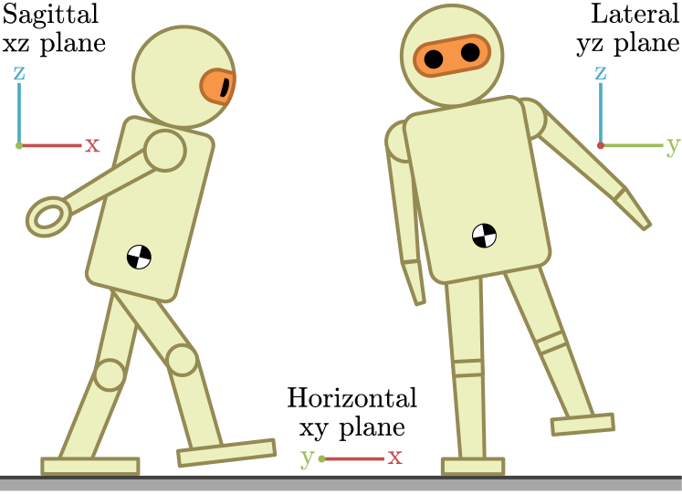
Figure 6: The relevant major planes for the application of bipedal walking. The fused yaw parameter $\psi\equiv p_{z}$ describes the heading of the robot, the fused pitch $\theta$ and tilt phase $p_{y}$ relate to the sagittal component of orientation of the robot, and the fused roll $\phi$ and tilt phase $p_{x}$ relate to the lateral component of orientation of the robot. Using these parameters allows the motion, stability and state of balance of the robot to be evaluated, quantified and controlled separately in the three major planes.

Tilt rotations and the tilt phase space can be applied, with advantages, in many scenarios. For example, quadrotors in general need to tilt in the direction they wish to accelerate, so a smooth and axisymmetric way of representing such tilt, using a suitable mix of tilt angles, fused angles, and in particular the tilt phase space, can be of great benefit. Similar arguments for the use of these representations also apply to the scenarios of balance and bipedal locomotion, where the tilt rotation component is particularly relevant because it encapsulates the entire heading-independent balance state of the robot, with no extra component of rotation about the z-axis [5]. In fact, a tilted IMU accelerometer measures the direction of gravity, which is a direct measurement of $\tensor*[^{B}]{\mathbf{z}}{{}_{G}}$, the z-vector parameterisation of tilt rotations. This supports the notion that tilt rotations are a natural and meaningful split of orientations into yaw and tilt. Fig. 6 illustrates how for the application of bipedal walking the fused angles $\psi$, $\theta$, $\phi$ and/or the tilt phase space parameters $p_{x}$, $p_{y}$, $p_{z}$ can be used to independently quantify the amount of rotation in each of the three major planes. This allows the motion, stability and state of balance to be measured and controlled separately in each of these three planes, which correspond to the sagittal, lateral and horizontal, i.e. heading, planes of walking.

Due to the many advantageous properties of the tilt phase space (see Section V-C), and in particular due to magnitude axisymmetry, the tilt phase space was chosen as the basis of a developed feedback controller for the stabilisation of bipedal walking [2]. It is in the nature of feedback controllers, e.g. PID-style controllers, to produce control inputs of arbitrary magnitude based on a set of gains, so the unbounded nature of the tilt phase space was able to be utilised to full effect.

The concepts of tilt rotations and the tilt phase space have also been applied in the keypoint gait generator that underlies the feedback gait presented in [2]. Most notably, the tilt phase space is used to separate the yaw and tilt of the feet at each gait keypoint, and then interpolate between them using the orientation cubic spline interpolation described in Section V-E. This ensures that the yaw and tilt profiles are individually exactly as intended in the final 3D foot trajectories, especially seeing as the yaw profiles come from the commanded step sizes, and the tilts come separately from the feedback controller. Tilt vector addition is also required, because multiple feedback components need to contribute to each final foot tilt. The summated foot tilts are not guaranteed to be in range though, so the unbounded nature of the tilt phase space helps in being robust to ‘wrapping around’ prior to saturation. All this allows effective and robust gait trajectories to be generated for robots using this method.

VIII Conclusion

Both tilt rotations and the novel tilt phase space were formally introduced in this paper. As was shown in detail, tilt rotations possess many remarkable properties, and are useful for the analysis of the rotations of rigid bodies, in particular balancing bodies. The value of the tilt phase space was demonstrated, firstly in that it provides a tool to study unbounded tilt rotations in a way analogous to fused angles for orientations, and secondly in that it formalises a vector space of tilt rotations that allows for intuitive commutative addition. The tilt phase space also enables more complex operations, such as for example cubic spline interpolation in a way that cleanly respects the independence of yaw and tilt. As a final note, all rotation representations that were presented in this paper have open source software library support, in both C++ and Matlab (see Section I).

References

- [1] P. Allgeuer and S. Behnke, “Fused Angles: A representation of body orientation for balance,” in Int. Conf. on Intelligent Robots and Systems (IROS), Hamburg, Germany, 2015.
- [2] P. Allgeuer and S. Behnke, “Bipedal walking with corrective actions in the tilt phase space,” in Proceedings of 18th Int. Conf. on Humanoid Robots (Humanoids), Beijing, China, 2018.
- [3] P. Allgeuer and S. Behnke, “Omnidirectional bipedal walking with direct fused angle feedback mechanisms,” in Proceedings of 16th Int. Conf. on Humanoid Robots (Humanoids), Cancún, Mexico, 2016.
- [4] H. Farazi, P. Allgeuer, G. Ficht, and S. Behnke, “Nimbro teensize team description 2016,” University of Bonn, Tech. Rep., 2016.
- [5] P. Allgeuer and S. Behnke, “Fused angles and the deficiencies of Euler angles,” in Int. Conf. on Intell. Robots and Systems (IROS), 2018.
- [6] B. Palais, R. Palais, and S. Rodi, “A disorienting look at Euler’s theorem on the axis of a rotation,” The American Mathematical Monthly, pp. 892–909, 2009.
- [7] O. Bauchau and L. Trainelli, “The vectorial parameterization of rotation,” Nonlinear Dynamics, vol. 32, no. 1, pp. 71–92, 2003.
- [8] L. Trainelli and A. Croce, “A comprehensive view of rotation parameterization,” in Proceedings of ECCOMAS, 2004.
- [9] J. Argyris, “An excursion into large rotations,” Computer Methods in Applied Mechanics and Engineering, vol. 32, pp. 85–155, 1982.
- [10] I. G. Kang and F. C. Park, “Cubic spline algorithms for orientation interpolation,” International Journal for Numerical Methods in Engineering, vol. 46, no. 1, pp. 45–64, 1999.