Entanglement detection by violations of noisy uncertainty relations:
A proof of principle
Abstract
It is well-known that the violation of a local uncertainty relation can be used as an indicator for the presence of entanglement. Unfortunately, the practical use of these non-linear witnesses has been limited to few special cases in the past. However, new methods for computing uncertainty bounds became available. Here we report on an experimental implementation of uncertainty-based entanglement witnesses, benchmarked in a regime dominated by strong local noise. We combine the new computational method with a local noise tomography in order to design noise-adapted entanglement witnesses. This proof-of-principle experiment shows that quantum noise can be successfully handled by a fully quantum model in order to enhance entanglement detection efficiencies.
pacs:
123 456Introduction
Entanglement is a crucial resource that enables quantum technologies like cryptography, computing, dense coding and many more. Hence, in addition to the challenging task of creating entanglement Einstein et al. (1935); Aspect et al. (1982); Kwiat et al. (1995); Pan et al. (1998); Werner (1989); Yin et al. (2017), robust and practical verification schemes are a key requirement for unleashing the full power of these technologies.
In this letter we report a proof-of-principle experiment of noise-tolerant non-linear entanglement witnesses which are based on violations of local uncertainty relations. In our implementation, we detect photon encoded qutrit-qutrit entanglement by local measurements of orthogonal angular momentum components affected by strong noise originating from random spin-flips. We adapt our witnesses to this noise by an error estimation solely based on local measurements. We successfully benchmark our detection scheme in a noise regime where conventional witnesses fail to detect any entanglement at all (see Fig. 1).
The existence of unavoidable uncertainties in any quantum measurement process Heisenberg (1927); Kennard (1927); Dammeier et al. (2015); Rozpędek et al. (2016); Schrödinger (1930); Maassen and Uffink (1988); Abdelkhalek et al. (2015); Deutsch (1983); Busch et al. (2014); Zhao et al. (2017); Jia et al. (2017); Maccone and Pati (2014); Riccardi et al. (2017a); Schwonnek (2018); de Guise et al. (2018) is one of the most characteristic implications of quantum physics. It has been known for quite a while Hofmann and Takeuchi (2003); Gühne and Tóth (2009); Gühne (2004); Wang et al. (2007); Costa Sprotte et al. (2017); Riccardi et al. (2017b) that any variance-based uncertainty relation
| (1) |
on local measurements and yields a non-linear entanglement witness. Unfortunately, in the past, this method could only be applied in a very limited context because explicit bounds in (1) were only known for few symmetrical cases (see e.g. Schwonnek et al. (2017) for a list). However, a method for computing bounds for general and recently became available Schwonnek et al. (2017); Szymański and Zyczkowski (2018).
For our experiment, we employ a modified version of this method in order to handle the influence of quantum noise entirely on a quantum level, whenever a quantum model of this noise is available. In practice, we first motivate a noise model by theory and check it on a large range of tomographic test states afterwards. Thereby we concentrate on local noise sources Streltsov et al. (2011), since they are accessible in any LOCC setting.
The wider scope of our proof-of-principle experiment are applications in long-range communication settings Yin et al. (2017); Dür et al. (1999); Bratzik et al. (2013). Here, local noise typically turns out to be the actual limitation in practice, even though in theory, the exponential scaling of absorption is considered to be the limiting factor Brassard et al. (2000); Briegel et al. (1998).
I Methods
Non-linear entanglement witnesses based on uncertainty relations.— In general, an entanglement witness is any separating functional that can be used to distinguish an entangled state from separable states Gühne and Tóth (2009). More precisely, by taking the infimum of such a functional over all separable states, i.e. states of the form
| (2) |
we obtain a constant
| (3) |
which allows us to witness entangled states, i.e. states that are not of the form (2) Werner (1989): if we find that , we immediately know that cannot be a separable state and is therefore entangled.
Typically linear functionals are considered. In contrast, the entanglement witnesses we are using in our experiment are based on variances of measurements and and therefore non-linear. Explicitly, we use weighted uncertainty sums given by the functional
| (4) |
where . Here, are the so-called moment operators given for general POVMs Heinosaari and Ziman (2011) as follows: Let be an outcome of and the corresponding POVM element, then the -th moment operator of is given by .
From an experimental perspective, our witnesses have the advantage that only the first two moments of an outcome distribution are needed. In contrast to the full outcome statistics, these moments can be estimated with much higher precision given a finite sample.
From a theoretical perspective, the corresponding constant plays the role of a sum of local uncertainty bounds: Consider a setting where two parties, named Alice and Bob, can both choose between two measurements and . We then have four local measurements, and for Alice and and for Bob. Globally, the -th moment of the -measurement is then given by
| (5) |
and similar for .
The chosen witness has some convenient properties with regard to calculating the infimum in equation (3): Since it is a concave function which we want to minimize over a convex set (the set of all separable states), the optima are obtained at extreme points. However, the extreme points of the set of separable states are pure states, i.e. we only have to find the infimum over all product states. The variance is then additive:
| (6) |
which leads to the following expression for the uncertainty bound:
| (7) | ||||
| (8) |
Hence, we only need bounds on the functional with respect to local measurements and states.
Local noise.— For the design of noise robust entanglement witnesses, we abstract the action of any local noise source as depicted in Fig. 2: Whenever a particle enters a local lab, it is firstly affected by local noise, i.e. it has to cross a channel , before it hits an idealized detector .
From the perspective of the Schrödinger picture this results in a disturbed state , which then results in disturbed measurement outcomes with disturbed moments:
| (9) |
Generically, these moments lead to an increase of the uncertainty , which reflects the negative effect of the noise. Hence entanglement, which was present in the initial state , may no longer be detectable by a witness based on the local uncertainty of the ideal measurement .
At this point we should keep in mind that, from a mathematical perspective, the disturbed state still contains a lot of information about the undisturbed input . Here one strategy could be to implement an error-correcting quantum channel , which is unfortunately not practical: beside the fact that this would demand a very high level of quantum control, a full recovery of an unknown is usually not possible since the inverse of a noise channel is typically not a -map which means that it is not a valid quantum operation.
This fundamental shortcoming can be circumvented by representing the noise in the Heisenberg picture: From this perspective, only the local detectors are affected by the noise. Here, we can assume that the characteristics of an ideal detector are well known in advance, such that we can directly describe noisy measurements by a POVM with elements
| (10) |
and moments
| (11) |
Here, the local noise is compensated on a classical level when we adapt our entanglement witnesses by using the correct local uncertainty bounds for disturbed measurements . In practice this demands us to (i) collect information on the local noise in order to come up with a valid error model and (ii) compute the corresponding uncertainty bounds. We achieved the first task by performing measurements on (local) test-states and the second by using the recently developed algorithm from Schwonnek et al. (2017), which can also be applied to arbitrary POVMs.
II Experiment
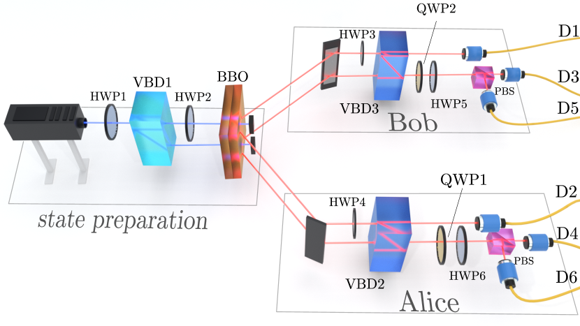
Setup.— In our implementation, entanglement is realized by so called path polarization hybrid states Hu et al. (2016, 2018). Due to many developments in recent years, the path and the polarization degrees of freedom of a photon can be controlled easily and efficiently.
We use the setup as sketched in Fig. 3 to prepare the singlet state
| (12) |
We detect the entanglement of this state based on measurements of spin-1 angular momentum components and .
The noise model.— In our experiment we probe qutrit-qutrit entanglement detected by local measurements of the spin-1 components and . In order to benchmark the performance of our method in a regime where the conventional criteria fail to work, we actively add local noise to our measurements.
We generate this noise by applying a random sequence of local spin-flips within the plane. For a noise parameter which corresponds to an effective spin-flip probability this implements a channel
| (13) |
where an individual spin-flip is described by the unitary .
For this channel the operators and , corresponding to the first moments of our noisy detectors, are given by
| (14) | ||||
| (15) |
whereas the operators for the second moments stay unchanged, i.e. we have
| (16) |
Given this noise model we probe the actual local noise by checking the predicted local uncertainty relations on a set of test states
| (17) |
The results of this are depicted in Fig. 4.
For each state we collect about photons in total. The statistical errors caused by the fluctuation of the coincidence count stay below and , which is too small to be depicted in the figures.
In principle, our method provides the ability to incorporate more sophisticated noise models than the presented one. However, for this experiment, it turns out that the dominant part of the noise regime can be well explained (see Fig. 4) by the action of the channel (13), with a spin-flip noise parameter , estimated from experimental data.
Entanglement detection.—
Via the procedure described above, we can do measurements on a state which is, in principle, unknown but close to the singlet state (12). The singlet state has the highest entanglement which yields the highest violation of the computed bounds, hence it is favourable to use this state for the purpose of benchmarking.
The operators we measure are
| (18) | ||||
| (19) |
for , i.e. the first two moments of the total angular momentum (see also Lücke et al. (2014) for similar applications on BECs). The noisy operators are defined analogously.
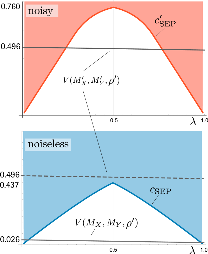
The measurement is performed once without noise and once with noise. The major advantage of our scheme is that we can already test a variety of witnesses, i.e. all values of and in our witness functional (4), by performing a measurement of only two spin components ( and ). More precisely, we measure a variance tuple (), from which the values of the variance functional can be computed for all . Whenever this functional violates an uncertainty bound, that is we observe
| (20) |
for some choice of parameters, entanglement is detected.
The results of this are shown in Fig. 5, where we used, without loss of generality, the parameterization . We detect entanglement with witnesses in the ranges and , for the noiseless and the noisy case, respectively. Remarkably, we observe for the noisy case that, even for the highly entangled state we used here, the non-adapted witness would fail to detect any entanglement (for any ), as shown by the placement of the dashed line in Fig. 5.
Furthermore, the strongest witness for this particular state is given by the parameters . Here we obtain the uncertainty bounds
| (21) |
and
| (22) |
III conclusion
We described a proof of principle experiment that demonstrates that high precision experimental techniques and improved computational methods can be merged to turn a simple idea Hofmann and Takeuchi (2003) into a practical technology.
The local noise in this experiment has a relatively simple appearance, but our techniques are not limited to this: A clear direction for future work is to use this scheme for an improvement of existing entanglement distribution setups, especially in long range settings. It is also worth mentioning that our scheme can be extended to settings with more than two local measurements as well. Beside experimental challenges, this also demands new numerical methods. For this case, the corresponding uncertainty relations are way less investigated than in the case of two measurements. Here, new numerical methods and experimental tests would contribute a lot to the understanding of this case.
Acknowledgements.
R.S. and R.W. thank Reinhard F. Werner, Tobias J. Osborne, and Deniz E. Stiegemann for fruitful discussions and critically reading our manuscript. Y.Y.Z. thanks Yu Guo’s help in the experiment. R.S. and R.W. also acknowledge the financial support given by the RTG 1991 and the CRC 1227 DQ-mat funded by the DFG, the collaborative research project Q.com-Q funded by the BMBF and the Asian Office of Aerospace RD grant FA2386-18-1-4033. The work at USTC is supported by the National Natural Science Foundation of China under Grants (Nos.11574291, 11774334, 61327901,11874345 and 11774335), the China Postdoctoral Science Foundation (Grant No. BH2030000036), the National Key Research and Development Program of China (No.2017YFA0304100), and the Key Research Program of Frontier Sciences, CAS (No.QYZDY-SSW-SLH003), Anhui Initiative in Quantum Information Technologies.References
- Einstein et al. (1935) A. Einstein, B. Podolsky, and N. Rosen, Phys. Rev. 47, 777 (1935).
- Aspect et al. (1982) A. Aspect, J. Dalibard, and G. Roger, Phys. Rev. Lett. 49, 1804 (1982).
- Kwiat et al. (1995) P. G. Kwiat, K. Mattle, H. Weinfurter, A. Zeilinger, A. V. Sergienko, and Y. Shih, Phys. Rev. Lett. 75, 4337 (1995).
- Pan et al. (1998) J.-W. Pan, D. Bouwmeester, H. Weinfurter, and A. Zeilinger, Phys. Rev. Lett. 80, 3891 (1998).
- Werner (1989) R. F. Werner, Phy. Rev. A 40, 4277 (1989).
- Yin et al. (2017) J. Yin, Y. Cao, Y.-H. Li, S.-K. Liao, L. Zhang, J.-G. Ren, W.-Q. Cai, W.-Y. Liu, B. Li, H. Dai, et al., Science 356, 1140 (2017).
- Heisenberg (1927) W. Heisenberg, Z. Phys. 43, 172 (1927).
- Kennard (1927) E. H. Kennard, Z. Phys. 44, 326 (1927).
- Dammeier et al. (2015) L. Dammeier, R. Schwonnek, and R. Werner, New J. Phys. 9, 093946 (2015), arXiv:1505.00049.
- Rozpędek et al. (2016) F. Rozpędek, J. Kaniewski, P. J. Coles, and S. Wehner, New J. Phys. 19, 023038 (2016), arXiv:1606.05565.
- Schrödinger (1930) E. Schrödinger, Sitzungsber. Preuss. Akadem. Wiss., Physikalisch-mathematische Klasse , 296 (1930).
- Maassen and Uffink (1988) H. Maassen and J. B. M. Uffink, Phys. Rev. Lett. 60, 1103 (1988).
- Abdelkhalek et al. (2015) K. Abdelkhalek, R. Schwonnek, H. Maassen, F. Furrer, J. Duhme, P. Raynal, B. Englert, and R. Werner, Int. J. Quant. Inf. 13, 1550045 (2015), arXiv:1509.00398.
- Deutsch (1983) D. Deutsch, Phys. Rev. Lett. 50, 631 (1983).
- Busch et al. (2014) P. Busch, P. Lahti, and R. F. Werner, J. Math. Phys. 55, 042111 (2014), arXiv:1312.4392.
- Zhao et al. (2017) Y.-Y. Zhao, P. Kurzyński, G.-Y. Xiang, C.-F. Li, and G.-C. Guo, Phys. Rev. A 95, 040101 (2017).
- Jia et al. (2017) Z.-A. Jia, Y.-C. Wu, and G.-C. Guo, Phys. Rev. A 96, 032122 (2017), arXiv:1705.08825.
- Maccone and Pati (2014) L. Maccone and A. Pati, Phys. Rev. Lett. 113, 260401 (2014).
- Riccardi et al. (2017a) A. Riccardi, C. Macchiavello, and L. Maccone, Phys. Rev. A 95, 032109 (2017a), arXiv:1701.04304.
- Schwonnek (2018) R. Schwonnek, Quantum 2, 59 (2018).
- de Guise et al. (2018) H. de Guise, L. Maccone, B. C. Sanders, and N. Shukla, (2018), arXiv:1804.06794.
- Hofmann and Takeuchi (2003) H. F. Hofmann and S. Takeuchi, Phys. Rev. A. 68, 032103 (2003).
- Gühne and Tóth (2009) O. Gühne and G. Tóth, Phys. Rep. 474, 1 (2009).
- Gühne (2004) O. Gühne, Detecting quantum entanglement: entanglement witnesses and uncertainty relations, Ph.D. thesis, Universität Hannover (2004).
- Wang et al. (2007) Z.-W. Wang, Y.-F. Huang, Y.-S. Ren, X.-F. Zhang, and G.-C. Guo, Eur. Phys. Lett. 78, 40002 (2007).
- Costa Sprotte et al. (2017) A. C. Costa Sprotte, R. Uola, and O. Gühne, (2017), arXiv:1710.04541.
- Riccardi et al. (2017b) A. Riccardi, C. Macchiavello, and L. Maccone, (2017b), arXiv:1711.09707.
- Schwonnek et al. (2017) R. Schwonnek, L. Dammeier, and R. Werner, Phys. Rev. Lett. 119, 170404 (2017), arXiv:1705.10679.
- Szymański and Zyczkowski (2018) K. Szymański and K. Zyczkowski, (2018), arXiv:1804.06191.
- Streltsov et al. (2011) A. Streltsov, H. Kampermann, and D. Bruß, Phys. Rev. Lett. 107, 170502 (2011).
- Dür et al. (1999) W. Dür, H.-J. Briegel, J. Cirac, and P. Zoller, Phys. Rev. A 59, 169 (1999).
- Bratzik et al. (2013) S. Bratzik, S. Abruzzo, H. Kampermann, and D. Bruß, Phys. Rev. A 87, 062335 (2013).
- Brassard et al. (2000) G. Brassard, N. Lütkenhaus, T. Mor, and B. C. Sanders, Phys. Rev. Lett. 85, 1330 (2000).
- Briegel et al. (1998) H.-J. Briegel, W. Dür, J. Cirac, and P. Zoller, Phys. Rev. Lett. 81, 5932 (1998).
- Heinosaari and Ziman (2011) T. Heinosaari and M. Ziman, The mathematical language of quantum theory: from uncertainty to entanglement (Cambridge University Press, 2011).
- Hu et al. (2016) X.-M. Hu, J.-S. Chen, B.-H. Liu, Y. Guo, Y.-F. Huang, Z.-Q. Zhou, Y.-J. Han, C.-F. Li, and G.-C. Guo, Phys. Rev. Lett. 117, 170403 (2016).
- Hu et al. (2018) X.-M. Hu, B.-H. Liu, Y. Guo, G.-Y. Xiang, Y.-F. Huang, C.-F. Li, G.-C. Guo, M. Kleinmann, T. Vértesi, and A. Cabello, Phys. Rev. Lett. 120, 180402 (2018).
- Lücke et al. (2014) B. Lücke, J. Peise, G. Vitagliano, J. Arlt, L. Santos, G. Tóth, and C. Klempt, Phys. Rev. Lett. 112, 155304 (2014), arXiv:1403.4542.