Abstract

Correlated pattern mining has increasingly become an important task in data mining since these patterns allow conveying knowledge about meaningful and surprising relations among data. Frequent correlated patterns were thoroughly studied in the literature.

In this thesis, we propose to benefit from both frequent correlated as well as rare correlated patterns according to the bond correlation measure. Nevertheless, a main moan addressed to correlated pattern extraction approaches is their high number which handicap their extensive utilizations. In order to overcome this limit, we propose to extract a subset without information loss of the sets of frequent correlated and of rare correlated patterns, this subset is called “Condensed Representation“. In this regard, we are based on the notions derived from the Formal Concept Analysis FCA, specifically the equivalence classes associated to a closure operator $f_{bond}$ dedicated to the bond measure, to introduce new concise representations of both frequent correlated and rare correlated patterns. We then design the new mining approach, called Gmjp, allowing the extraction of the sets of frequent correlated patterns, of rare correlated patterns and their associated concise representations. In addition, we present the Regenerate algorithm allowing the query of the $\mathcal{RCPR}$ condensed representation associated to the $\mathcal{RCP}$ set as well as the RcpRegeneration algorithm dedicated to the regeneration of the whole set of rare correlated patterns from the $\mathcal{RCPR}$ representation.

The carried out experimental studies highlight the very encouraging compactness rates offered by the proposed concise representations and prove the good performance of the Gmjp algorithm. To improve the obtained performance, we introduced and evaluated the optimized version of Gmjp. The latter shows much better performances than do the initial version of Gmjp. In order to prove the usefulness of the extracted condensed representation, we conduct a classification process based on correlated association rules derived from closed correlated patterns and their associated minimal generators. The obtained rules were applied to the context of intrusion detection and achieve encouraging results.

Key Words: Formal Concept Analysis, Constraint Data Mining, Monotonicity, Anti-monotonicity, bond Correlation Measure, Itemset Extraction, Condensed Representation, Classification, Associative Rule.

Résumé

La fouille des motifs corrélés est une piste de recherche de plus en plus attractive en fouille de données grâce à la qualité et à l’utilité des connaissances offertes par ces motifs. Plus précisément, les motifs fréquents corrélés ont été largement étudiés auparavant dans la littérature.

Notre objectif dans cette thèse est de bénéficier à la fois des connaissances offertes par les motifs corrélés fréquents ainsi que les motifs rares corrélés selon la mesure de corrélation bond. Cependant, un principal problème est lié à la fouille des motifs corrélés concerne le nombre souvent très élevé des motifs corrélés extraits. Un tel nombre handicape une exploitation optimale et aisée des connaissances encapsulées dans ces motifs. Pour pallier ce problème, nous nous intéressons dans cette thèse à l’extraction d’un sous-ensemble, sans perte d’information, de l’ensemble de tous les motifs corrélés. Ce sous-ensemble, le noyau d’itemsets, appelé “Représentations Concises”, à partir duquel tous les motifs redondants peuvent être régénérés sans perte d’informations. Le but d’une telle représentation est de minimiser le nombre de motifs extraits tout en préservant les connaissances cachées et pertinentes.

Afin de réaliser cet objectif, nous nous sommes basés sur les notions dérivées de l’analyse formelle de concepts AFC. Plus précisément, les représentations condensées, que nous proposons, sont issues des notions de classes d’équivalence induites par l’opérateur de fermeture $f_{bond}$ associé à la mesure de corrélation bond. Après la caractérisation des représentations condensées proposées, nous introduisons l’algorithme Gmjp dédié à l’extraction des motifs corrélés fréquents, des motifs corrélés rares ainsi que leurs représentations condensées associées. Nous présentons également l’algorithme Regenerate d’interrogation de la représentation $\mathcal{RCPR}$ associée à l’ensemble $\mathcal{RCP}$ des motifs corrélés rares et nous proposons aussi l’algorithme RCPRegeneration dédié à la régénération de l’ensemble total des motifs corrélés rares à partir de la représentation concise $\mathcal{RCPR}$.

L’évaluation expérimentale menée met en valeur les taux de compacités très intéressants offerts par les différentes représentations concises proposées et justifie également les performances encourageantes de l’approche Gmjp. Afin d’améliorer les performances de l’algorithme Gmjp, nous proposons une version optimisée de Gmjp. Cette version optimisée présente des temps d’exécution beaucoup plus réduits que la version initiale. De plus, nous avons conduit un processus de classification associative basé sur les règles associatives corrélées dérivées à partir des motifs corrélés fermés et de leurs générateurs minimaux. Les résultats de classification des données de détection d’intrusions, sont très encourageants et ont prouvé une grande utilité de la fouille des motifs corrélés.

Mots Clés : Analyse Formelle de Concept, Fouille sous Contraintes, Monotonie, Anti-monotonie, Mesure bond, Extraction de motifs, Représentation concise, Classification, Règles associatives.

List of Algorithms

loa

Chapter 1 Introduction

1.1 Introduction and Motivations

The development of new information and communication technologies and the globalization of markets make the competition more and more increased among companies. In this sense, the need for access to an accurate information for decision-making is increasingly urgent. The actual problem is linked to lack of access to relevant information in the presence of the large amount of data. The collected data in various fields are becoming larger. This motivates the need to analyze and interpret data in order to extract useful knowledge.

In this context, the process of knowledge discovery from databases (KDD) is a complete process aiming to extract useful, hidden knowledge from huge amount of data [Agrawal and Srikant, 1994]. Data Mining is one of the main steps of this process and is dedicated to offer the necessary tools needed for an optimal exploration of data. Many state of the art approaches were focused on frequent itemset extraction and association rule generation. Nevertheless, two main problems handicap the good use of the returned knowledge from the set of frequent itemsets. The first problem is related to the quality of the offered knowledge since the degree of correlation of the extracted itemsets may be not interesting for the end user. The second problem is related often to the huge quantity of the extracted knowledge.

To overcome these problems, many previous works propose to integrate the correlation measures within the mining process [Brin et al., 1997, Lee et al., 2003, Omiecinski, 2003, Kim et al., 2004, Xiong et al., 2006]. Correlated pattern mining is then shown to be more complex but more informative than traditional frequent patterns mining. In fact, correlated patterns offer a precise information about the degree of apparition of the items composing a given itemset [Segond and Borgelt, 2011]. This key information specifies the simultaneous apparition frequency among items, i.e., their co-occurrence, as well as their apparition frequency, i.e., their occurrence.

Other state of the art approaches deal with the extraction of a subset, without information loss, of the whole set of correlated patterns. This subset, is named, “Condensed Representation“ and from which we are able to derive all the redundant correlated patterns. The condensed representations prove their high utility in different fields such as: bioinformatics [Martinez et al., 2009] and data grids [Hamrouni et al., 2015].

The main objective behind defining such a condensed representation is to reduce the number of the extracted patterns while preserving the same amount of pertinent knowledge. In addition to this, all of the extracted associated rules, derived from correlated patterns fulfilling a correlation measure such as all-confidence or bond, are valid with respect to minimal support and to minimal confidence thresholds [Omiecinski, 2003].

Frequent correlated itemset mining was then shown to be an interesting task in data mining. Since its inception, this key task grasped the interest of many researchers since it meets the needs of experts in several application fields [Ben Younes et al., 2010], such as market basket study. However, the application of correlated frequent patterns is not an attractive solution for some other applications, e.g., intrusion detection, analysis of the genetic confusion from biological data, detection of rare diseases from medical data, to cite but a few [Koh and Rountree, 2010, Mahmood et al., 2010, Romero et al., 2010, Szathmary et al., 2010, Manning et al., 2008]. As an illustration of the rare correlated patterns applications in the field of medicine, the rare combination of symptoms can provide useful insights for doctors.

To the best of our knowledge, there is no previous work that dealt with both frequent correlated as well as rare correlated patterns according to a specified correlation metric. Thus, motivated by this issue, we propose in this thesis to benefit from the knowledges returned from both frequent correlated as well as rare correlated patterns according to the bond correlation measure. To solve this challenging problem, we propose an efficient algorithmic framework, called GMJP, allowing the extraction of both frequent correlated patterns, rare correlated patterns as well as their associated concise representations.

1.2 Contributions

Our first contribution consists in defining and studying the characteristics of the condensed representations associated to frequent correlated as well as the condensed representations associated to rare correlated ones. In this respect, we are based on the notions derived from the Formal Concept Analysis (FCA) [Ganter and Wille, 1999], specifically the equivalence classes associated to a closure operator $f_{bond}$ dedicated to the bond measure to introduce our new concise representations of both frequent correlated and rare correlated patterns. The first concise representation $\mathcal{RCPR}$ associated to the $\mathcal{RCP}$ set of rare correlated patterns, is composed by the maximal elements of the rare correlated equivalence classes, called “Closed Rare Correlated Patterns $\mathcal{CRCP}$ set“ union of their associated minimal generators called “Minimal Rare Correlated Patterns $\mathcal{MRCP}$ set“. Two other optimizations of the $\mathcal{RCPR}$ representation are also proposed. The first optimization is composed by the whole set $\mathcal{CRCP}$ of closed rare correlated patterns union of the minimal elements of the $\mathcal{MRCP}$ set. The second optimization is composed by the maximal elements of the $\mathcal{CRCP}$ of closed rare correlated patterns union of the whole $\mathcal{MRCP}$ set. We prove that both of these representations are also concise and exact. Our third optimized representation is a condensed approximate representation. The latter is composed by the maximal elements of the $\mathcal{CRCP}$ set union of the minimal elements of the $\mathcal{MRCP}$ set. According to the $\mathcal{FCP}$ set of frequent correlated patterns, the condensed exact representation is composed by the Closed Correlated Frequent Patterns. We prove the theoretical properties of accuracy and compactness of all the proposed representations.

Our second contribution is the design and the implementation of a new mining approach, called Gmjp, allowing the extraction of the sets of frequent correlated patterns, of rare correlated patterns and their associated concise representations. Gmjp is a sophisticated mining approach that allows a simultaneous integration of two opposite paradigms of monotonic and anti-monotonic constraints. In addition, we present the Regenerate algorithm allowing the query of the $\mathcal{RCPR}$ condensed representation associated to the $\mathcal{RCP}$ set as well as the RcpRegeneration algorithm dedicated to the regeneration of the whole set of rare correlated patterns from the $\mathcal{RCPR}$ representation.

Our third contribution consists in proposing an optimized version of Gmjp. The latter shows much better performance than the initial version of Gmjp. In order to prove the usefulness of the extracted condensed representation, we conduct a classification process based on correlated association rules derived from closed correlated patterns and their associated minimal generators. The obtained rules are applied to the context of intrusion detection and achieve promoting results.

The evaluation protocol of our approaches consists in experimental studies carried out over dense and sparse benchmark datasets commonly used in evaluating data mining contributions. The evaluation of the classification process is based on the KDD 99 database of intrusion detection data. We also conduct the process of applying the $\mathcal{RCPR}$ representation on the extraction of rare correlated association rules from Micro-array gene expression data related to Breast-Cancer. The diverse obtained association-rules reveals a variety of relationship between up and down regulated gene-expressions.

1.3 Thesis Organization

The remainder of this thesis is organized as follows:

Chapter 2 introduces the basic notions related to the itemset search space and to itemset extraction. We also define two distinct categories of constraints: monotonic and anti-monotonic. We equally introduce the environment of Formal Concept Analysis (FCA) which offers the basis for the proposition of our approaches, specifically the notions of Closure Operator, Minimal Generator, Closed Pattern, Equivalence class and Condensed representation of a set of patterns.

Chapter 3 offers an overview of the state of the art approaches dealing with correlated patterns mining. We start this chapter by defining the most used correlation measures. Then, we continue with the approaches related to frequent correlated patterns, followed by the state of the art of rare correlated patterns then the overview of the algorithms focusing on condensed representations of correlated patterns.

Chapter 4 focuses on characterizing the $\mathcal{FCP}$ set of frequent correlated patterns as well as the $\mathcal{RCP}$ set of rare correlated patterns. It introduces the condensed exact and approximate representations associated to the $\mathcal{RCP}$ set as well as the concise exact representation associated to the $\mathcal{FCP}$ set. The main content of this chapter was published in [Bouasker et al., 2012b] and in [Bouasker et al., 2015].

Chapter 5 introduces the Gmjp approach, allowing the extraction of the sets of frequent correlated patterns, of rare correlated patterns and their associated concise representations. The optimized version of Gmjp, named Opt-Gmjp, was also presented. This chapter also presents the theoretical complexity approximation of Gmjp. In addition, this chapter describes the Regenerate algorithm allowing the query of the $\mathcal{RCPR}$ condensed representation associated to the $\mathcal{RCP}$ set as well as the RcpRegeneration algorithm dedicated to the regeneration of the whole set of rare correlated patterns from the $\mathcal{RCPR}$ representation. The main content of this chapter was published in [Bouasker et al., 2012a] and in [Bouasker et al., 2015].

Chapter 6 focuses on the experimental validation of the proposed approaches. The evaluation process is based on two main axes, the first is related to the compactness rates of the condensed representations while the second axe concerns the running time. This chapter evaluates the optimized version of Gmjp, which presents much better performance than do Gmjp over different benchmark datasets. The content related to the optimizations and evaluations was published in [Bouasker and Ben Yahia, 2015].

Chapter 7 describes the classification process based on correlated patterns. This chapter starts by presenting the framework of association rule extraction, it clarifies the properties of the generic bases of association rules. Then, we continue with the detailed presentation of the application of both frequent correlated and rare correlated patterns within the classification of some UCI benchmark datasets. We equally present the application of rare correlated patterns in the classification of intrusion detection data from the KDD 99 dataset. The obtained results showed the usefulness of our proposed classification method over four different intrusion classes. This chapter is concluded with the application of the $\mathcal{RCPR}$ representation on the extraction of rare correlated association rules from Micro-array gene expression data. These extracted rules aims to identify relations among up and down regulated gene expressions. The main content of this chapter was published in [Bouasker et al., 2012c] and in [Bouasker and Ben Yahia, 2013].

Chapter 8 concludes the thesis and sketches out our perspectives for future work.

Part I Review of Correlated Patterns Mining

Chapter 2 Basic Notions

2.1 Introduction

The extraction of correlated patterns is shown to be more complex but more informative than traditional frequent patterns mining. In fact, these correlated patterns present a strong link among the items they compose and they prove their high utility in many real life applications fields.

This chapter is dedicated to the introduction of the basic notions needed for the presentation of our approaches. The second section deals with the basic notions related to the search space as well as the itemsets’s extraction. Then, we link in the third section with the presentation of the foundations of the formal concepts analysis (FCA) framework [Ganter and Wille, 1999]. The last section concludes the chapter.

2.2 Search Space

We begin by presenting the key notions related to itemset extraction, that will be used thorough this thesis. First, let us define an extraction context.

2.2.1 Extraction Context

Definition 1

Extraction Context
An extraction context (also called Context or Dataset) is represented by a triplet $\mathcal{C}$ = ($\mathcal{T},\mathcal{I},\mathcal{R}$) with $\mathcal{T}$ and $\mathcal{I}$ are, respectively, a finite sets of transactions (or objects) and of items (or attributes), and $\mathcal{R}$ $\subseteq$ $\mathcal{T}\times\mathcal{I}$ is a binary relation between the transactions and the items. A couple ($t$, $i$) $\in$ $\mathcal{R}$ if $t$ $\in$ $\mathcal{T}$ contains $i$ $\in$ $\mathcal{I}$.

Example 1

An example of an extraction context $\mathcal{C}$ $=$ ($\mathcal{T},\mathcal{I},\mathcal{R}$) is given by Table 2.1. In this context, the transaction set $\mathcal{T}=\{1,2,3,4,5\}$ (resp. the object set $\mathcal{O}=\{1,2,3,4,5\}$) and the items set $\mathcal{I}$ $=$ $\{$A, B, C, D, E,$\}$. The couple (2, B) $\in$ $\mathcal{R}$ since the transaction 2 $\in$ $\mathcal{T}$ contains the item B $\in$ $\mathcal{I}$.

	A	B	C	D	E
1	$\times$		$\times$	$\times$
2		$\times$	$\times$		$\times$
3	$\times$	$\times$	$\times$		$\times$
4		$\times$			$\times$
5	$\times$	$\times$	$\times$		$\times$

Table 2.1: An example of an Extraction Context $\mathcal{C}$.

Remark 1

We note, by sake of accuracy, that the notations of transactions database and extraction context have the same meaning thorough this thesis. They are denoted as $\mathcal{D}$ $=$ $\textsc{(}\mathcal{T},\mathcal{I},\mathcal{R}\textsc{)}$.

Definition 2

Itemset or Pattern
A transaction $t$ $\in$ $\mathcal{T}$, having an identifier denoted by TID (Tuple IDentifier), contains a non-empty set of items belonging to $\mathcal{I}$. A subset $I$ of $\mathcal{I}$ where $k$ $=$ $|I|$ is called a $k$-pattern or simply a pattern, and $k$ represents the cardinality of $I$. The number of transactions $t$ of a context $\mathcal{C}$ containing a pattern $I$, $|$$\{$ $t$ $\in$ $\mathcal{D}$ $|$ $I$ $\subseteq$ $t$$\}$$|$, is called absolute support of $I$ and is denoted $Supp\textsc{(}\wedge I\textsc{)}$. The relative support of $I$ or the frequency of $I$, denoted $freq\textsc{(}I\textsc{)}$, is the quotient of the absolute support by the total number of the transactions of $\mathcal{D}$, i.e., $freq\textsc{(}I\textsc{)}$ $=$ $\displaystyle\frac{\displaystyle{|{\{}t\in\mathcal{D}|I\subseteq t{\}}|}}{\displaystyle{|\mathcal{T}|}}$.

Remark 2

We point that, thorough this thesis, we are mainly interested in itemsets i.e. the set of items as a kind of patterns. Consequently, we use a form without separators to denote an itemset. For example, BD stands for the itemset composed by the items B and D.

2.2.2 Supports of a Pattern

To evaluate an itemset, many interesting measures can be used. The most common ones are presented by Definition 3.

Definition 3

Supports of a Pattern
Let $\mathcal{D}$=($\mathcal{T},\mathcal{I},\mathcal{R}$) an extraction context and a non empty itemset $I$ $\subseteq$ $\mathcal{I}$. We distinguish three kinds of supports for an itemset $I$ :

- The conjunctive support: Supp($\wedge$$I$) = $\mid$$\{$$t$ $\in$ $\mathcal{T}$ $\mid$ $\forall$ $i$ $\in$ $I$ : ($t$, $i$) $\in$ $\mathcal{R}$$\}$$\mid$

- The disjunctive support: Supp($\vee$$I$) = $\mid$$\{$$t$ $\in$ $\mathcal{T}$ $\mid$ $\exists$ $i$ $\in$ $I$ : ($t$, $i$) $\in$ $\mathcal{R}$$\}$$\mid$, and,

- The negative support: Supp($\neg$$I$) = $\mid$$\{$$t$ $\in$ $\mathcal{T}$ $\mid$ $\forall$ $i$ $\in$ $I$ : ($t$, $i$) $\notin$ $\mathcal{R}$$\}$$\mid$.

More explicitly, for an itemset $I$, the supports are defined as follows:

$\bullet$ Supp($\wedge$$I$): is equal to the number of transactions containing all the items of $I$.

$\bullet$ Supp($\vee$$I$): is equal to the number of transactions containing at least one item of $I$.

$\bullet$ Supp($\neg$$I$): is equal to the number of transactions that do not contain any item of $I$.

It is important to note that the “De Morgan” law ensures the transition between the disjunctive and the negative support of an itemset $I$ as follows : Supp($\neg$I) = $\mid\mathcal{T}\mid$ - Supp($\vee$I).

Example 2

Let us consider the extraction context given by Table 2.1 that will be used thorough the different examples. We have Supp($\wedge$AD) = $\mid$$\{$1$\}$$\mid$ = $1$, Supp($\vee$AD) = $\mid$$\{$ 1, 3, 5$\}$$\mid$ = $3$, and, Supp($\neg$(AD)) = $\mid$$\{$2, 4$\}$$\mid$ = $2$ ${}^{\textsc{(}}$.

In the following, if there is no risk of confusion, the conjunctive support will be simply denoted by support. Note that Supp($\wedge$$\emptyset$) = $|\mathcal{T}|$ since the empty set is included in all transactions, while Supp($\vee$$\emptyset$) = $0$ since the empty set does not contain any item. Moreover, $\forall$ $i$ $\in$ $\mathcal{I}$, Supp($\wedge$$i$) = Supp($\vee$$i$), while in the general case, for $I$ $\subseteq$ $\mathcal{I}$ and $I$ $\neq$ $\emptyset$, Supp($\wedge$$I$) $\leq$ Supp($\vee$$I$). A pattern $I$ is said to be frequent if Supp($\wedge$$I$) is greater than or equal to a user-specified minimum support threshold, denoted minsupp [Agrawal and Srikant, 1994]. The following lemma shows the links that exist between the different supports of a non-empty pattern $I$. These links are based on the inclusion-exclusion identities [Galambos and Simonelli, 2000].

Lemma 1

- Inclusion-exclusion identities - The inclusion-exclusion identities ensure the links between the conjunctive, disjunctive and negative supports of a non-empty pattern $I$.

$\textit{Supp}\textsc{(}\wedge I\textsc{)}\mbox{ }=\mbox{ }\displaystyle\sum_{\emptyset\subset I_{1}\subseteq I}{\textsc{(}-1\textsc{)}^{\mbox{$\mid I_{1}\mid$\mbox{ - 1}}}\mbox{ }\textit{Supp}\textsc{(}\vee I_{1}\textsc{)}}$	(1)
$\textit{Supp}\textsc{(}\vee I\textsc{)}\mbox{ }=\mbox{ }\displaystyle\sum_{\emptyset\subset I_{1}\subseteq I}{\textsc{(}-1\textsc{)}^{\mbox{$\mid I_{1}\mid$\mbox{ - 1}}}\mbox{ }\textit{Supp}\textsc{(}\wedge I_{1}\textsc{)}}$	(2)
$\textit{Supp}\textsc{(}\neg I\textsc{)}\mbox{ }=\mbox{ }\mid\mathcal{T}\mid\mbox{ }-\mbox{ }\textit{Supp}\textsc{(}\vee I\textsc{)}\mbox{ }\textsc{(}\mbox{The De Morgan's law}\textsc{)}$	(3)

2.2.3 Frequent Itemset - Rare Itemset - Correlated Itemset

Given a minimal threshold of support [Agrawal and Srikant, 1994], we distinguish between two kinds of patterns, frequent patterns and infrequent patterns (also called Rare patterns).

Definition 4

Frequent Itemset - Rare Itemset
Let an extraction context $\mathcal{C}$ = $\textsc{(}\mathcal{T},\mathcal{I},\mathcal{R}\textsc{)}$, a minimal threshold of the conjunctive support minsupp, an itemset $I$ $\subseteq$ $\mathcal{I}$ is said frequent if Supp($\wedge$$I$) $\geq$ minsupp. Otherwise, $I$ is said infrequent or rare.

Example 3

Let minsupp = 2. Supp($\wedge$BCE) = 3, the pattern BCE is a frequent pattern. However, the pattern CD is a rare pattern since Supp($\wedge$CD) = 1 $<$ 2.

In the following, we need to define the smallest rare patterns according to the relation of inclusion set. They correspond to rare patterns having all subsets frequent, and are defined as follows:

Definition 5

Minimal rare patterns
The $\mathcal{M}in\mathcal{RP}$ set of minimal rare patterns is composed of rare patterns having no rare proper subsets. This set is defined as: $\mathcal{M}in$$\mathcal{RP}$ = $\{I$ $\in$ $\mathcal{I}|$ $\forall$ $I_{1}\subset I$: Supp($\wedge I_{1}$) $\geq$ minsupp$\}$.

Example 4

Let us consider the extraction context sketched by Table 2.1. For minsupp = 4, we have $\mathcal{M}in\mathcal{RP}$ = $\{$$A$, $D$, $BC$, $CE$$\}$. $A$ and $D$ are minimal rare items, $BC$ is a minimal rare itemset since it is composed by two frequent items: $B$ with Supp($\wedge$B) = 4 and $C$ with Supp($\wedge$C) = 4.

In fact, in order to reduce the high number of frequent itemsets and to improve the quality of the extracted frequent itemets, other interesting measures apart from the conjunctive support are introduced within the mining process. These latter are called “Correlation Measures”. The itemsets fulfilling a given correlation measure are called “Correlated Itemsets”. This latter type of itemsets is defined in a generic way in what follows:

Definition 6

Correlated Itemset
Let a correlation measure M, a minimal correlation threshold minCorr, an itemset $I$ $\subseteq$ $\mathcal{I}$ is said correlated according to the measure M, if M($I$) $\geq$ minCorr. $I$ is said non correlated otherwise.

2.2.4 Categories of Constraints

Besides the minimal frequency constraint expressed by the minsupp threshold, other constraints can be integrated within the itemset’s extraction process. These constraints have two distinct types, “The monotonic constraints” and “The anti-monotonic constraints” [Bonchi and Lucchese, 2006].

Definition 7

Anti-monotonic Constraint
A constraint $Q$ is anti-monotone if $\forall$ $I$ $\subseteq$ $\mathcal{I}$, $\forall$ $I_{1}$ $\subseteq$ $I$ : $I$ fulfills $Q$ $\Rightarrow$ $I_{1}$ fulfills $Q$.

Definition 8

Monotone Constraint
A constraint $Q$ is monotone if $\forall$ $I$ $\subseteq$ $\mathcal{I}$, $\forall$ $I_{1}$ $\supseteq$ $I$ : $I$ fulfills $Q$ $\Rightarrow$ $I_{1}$ fulfills $Q$.

Example 5

The frequency constraint, i.e. having a support greater than or equal to minsupp, is an anti-monotonic constraint. In fact, $\forall$ $I$, $I_{1}$ $\subseteq$ $\mathcal{I}$, if $I_{1}$ $\subseteq$ $I$ and Supp($\wedge$$I$) $\geq$ minsupp, then Supp($\wedge$$I_{1}$) $\geq$ minsupp since Supp($\wedge$$I_{1}$) $\geq$ Supp($\wedge$$I$).

Dually, the constraint of rarity, i.e. having a support strictly lower than minsupp, is a monotonic constraint. In fact, $\forall$ $I$, $I_{1}$ $\subseteq$ $\mathcal{I}$, if $I_{1}$ $\supseteq$ $I$ and Supp($\wedge$$I$) $<$ minsupp, then Supp($\wedge$$I_{1}$) $<$ minsupp since Supp($\wedge$$I_{1}$) $\leq$ Supp($\wedge$$I$).

A set of itemset may fulfill different constraints simultaneously. Proposition 1, whose proof is in [Lee et al., 2006b], clarifies the conjunction of two constraints of the same nature.

Proposition 1

The conjunction of anti-monotonic constraints (resp. monotonic) is an anti-monotonic (resp. monotonic) constraint.

Let us define now the dual notions of order-ideal and order-filter [Ganter and Wille, 1999] defined on $\mathcal{P}\textsc{(}\mathcal{I}\textsc{)}$ and associated to the two kinds of constraints given by definitions 7 et 8.

Definition 9

Order Ideal
A subset $\mathcal{S}$ of $\mathcal{P}\textsc{(}\mathcal{I}\textsc{)}$ is an order ideal if it fulfills the following properties:

• If $I$ $\in$ $\mathcal{S}$, then $\forall$ $I_{1}$ $\subseteq$ $I$ : $I_{1}$ $\in$ $\mathcal{S}$.

• If $I$ $\notin$ $\mathcal{S}$, then $\forall$ $I$ $\subseteq$ $I_{1}$ : $I_{1}$ $\notin$ $\mathcal{S}$.

Definition 10

Order Filter
A subset $\mathcal{S}$ of $\mathcal{P}\textsc{(}\mathcal{I}\textsc{)}$ is an order filter if it fulfills the following properties:

• If $I$ $\in$ $\mathcal{S}$, then $\forall$ $I_{1}$ $\supseteq$ $I$ : $I_{1}$ $\in$ $\mathcal{S}$.

• If $I$ $\notin$ $\mathcal{S}$, then $\forall$ $I$ $\supseteq$ $I_{1}$ : $I_{1}$ $\notin$ $\mathcal{S}$.

An anti-monotone constraint such as the frequency constraint induces an order ideal on the itemset lattice. Dually, a monotonic constraint as the rarity constraint induces an order filter on the itemset lattice. The set of itemsets fulfilling a given constraint is called a Theory [Mannila and Toivonen, 1997]. This theory is delimited by two borders, the positive and the negative one, that are defined as follows:

Definition 11

Negative/Positive Border [Bonchi and Lucchese, 2006]
When considering an anti-monotonic constraint $C_{am}$, the border corresponds to the set of itemsets whose all subsets fulfill this constraint and whose all super-sets do not fulfill. Let a set of itemsets $\mathcal{S}$_am fulfilling an anti-monotonic constraint $C_{am}$, the border is formally defined as:

$\mathcal{B}d$($\mathcal{S}$_am) = $\{$$X$ $|$ $\forall$ $Y$ $\subset$ $X$ : $Y$ $\in$ $\mathcal{S}$_am and $\forall$ $Z$ $\supset$ $X$ : $Z$ $\notin$ $\mathcal{S}$_am$\}$

In the case of monotonic constraint $C_{m}$, the border corresponds to the set of patterns whose all supersets fulfills this constraint and whose all subsets do not fulfill.

Let a set of patterns $\mathcal{S}$_m fulfilling a monotonic constraint $C_{m}$, the border is formally defined as follows:

$\mathcal{B}d$($\mathcal{S}$_m) = $\{$$X$ $|$ $\forall$ $Y$ $\supset$ $X$ : $Y$ $\in$ $\mathcal{S}$_m and $\forall$ $Z$ $\subset$ $X$ : $Z$ $\notin$ $\mathcal{S}$_m$\}$

However, we have to distinguish for a given constraint $C$ between positive and negative borders. Let a set of patterns $\mathcal{S}$ fulfilling a constraint $C$. The positive border is denoted by $\mathcal{B}{d}^{+}\textsc{(}\mathcal{S}$) and corresponds to the patterns belonging to the border $\mathcal{B}{d}\textsc{(}\mathcal{S}$) and fulfilling the constraint $C$. The negative border is denoted by $\mathcal{B}{d}^{-}\textsc{(}\mathcal{S}$) and corresponds to the set of patterns belonging to the border $\mathcal{B}{d}\textsc{(}\mathcal{S}$) and not fulfilling the constraint $C$. These two borders are formally expressed as follows:

$\mathcal{B}{d}^{+}\textsc{(}\mathcal{S}\textsc{)}$ = $\mathcal{B}{d}\textsc{(}\mathcal{S}$) $\cap$ $\mathcal{S}$,

$\mathcal{B}{d}^{-}\textsc{(}\mathcal{S}\textsc{)}$ = $\mathcal{B}{d}\textsc{(}\mathcal{S}$) $\setminus$ $\mathcal{S}$.

In the next sub-section, we focus on the definition and the presentation of the notions related to condensed representations associated to a set of patterns.

2.2.5 Condensed Representations of a set of Patterns

The extraction of interesting patterns may be a costly operation in execution time and in memory consumption. This is due to the high number of the generated candidates. In this regard, an interesting issue consists in extracting sets of patterns with more reduced sizes. From which it is possible to regenerate the whole sets of patterns. These reduced sets are called “‘Condensed Representations”. In the case where the regeneration is performed in an exact way without information loss then the condensed representation is said exact. Otherwise, the condensed representation is said approximative. These representations are formally defined in what follows.

Definition 12

Condensed Representations [Mannila and Toivonen, 1997]
A concise representation of a set of interesting itemsets is a representative set allowing the characterization of the initial set in an exact or an approximative way.

Example 6

Let $\mathcal{R}$ be a concise representation of a set of frequent patterns $\mathcal{E}$. $\mathcal{R}$ is said concise exact representation, if starting from $\mathcal{R}$, we are able to determine for a given pattern whether it is a frequent pattern or not and to determine its conjunctive support also. For example, the closed frequent patterns [Pasquier et al., 2005] constitute a concise exact representation of the set of frequent itemsets.

Otherwise, $\mathcal{R}$ is a concise approximative representation of a set of patterns $\mathcal{S}$ if it is not able to exactly determine the support values of all the itemsets belonging to the $\mathcal{S}$ set. The representation $\mathcal{R}$ returns approximate values of these supports. For example, the maximal frequent itemsets [Roberto and Bayardo, 1998] constitute an approximative concise representation of the frequent patterns set. In fact, thanks to maximal frequent itemsets we are able to determine whether a given itemset is frequent or rare but it is not possible to exactly derive its conjunctive support value.

In general, a representation $\mathcal{R}$ constitutes “a perfect cover” if it fulfills the conditions established by the following definition:

Definition 13

Perfect Cover
A set $\mathcal{E}1$ is said a perfect cover of a set $\mathcal{E}$ if and only if $\mathcal{E}1$ allows to cover $\mathcal{E}$ without information loss and the size of $\mathcal{E}1$ never exceeds that of the set $\mathcal{E}$.

Various proposals aiming to reduce the size of a set of patterns $\mathcal{E}$ are based on the foundations of formal concepts analysis [Ganter and Wille, 1999]. The next section is dedicated to the presentation of the formal concept analysis’s framework.

2.3 Formal Concepts Analysis

2.3.1 Introduction

The formal concept analysis initially introduced by Wille in 1982 [Wille, 1982] treats formal concepts. A formal concept is a set of objects, The Extension, to which we applied a set of attributes, The Intention. The formal concept analysis provides a classification and an analysis tool whose principal element is the itemsets’s lattice defined as follows:

Definition 14

Itemsets’s Lattice
An itemsets’s lattice is a conceptual and hierarchical schema of patterns. It is also said lattice of set inclusion. In fact, the power set of $\mathcal{I}$ is ordered by set inclusion in the itemsets’ lattice.

This lattice shows the frequent itemsets, the rare ones as well as the $\mathcal{M}$in$\mathcal{RP}$ set of minimal rare patterns composing the positive border of the whole set of rare patterns.

2.3.2 Galois Connection

2.3.2.1. Closure Operator

In what follows, we present the fundamental basis of a closure operator.

Definition 15

Ordred Set
Let $E$ a set. A Partial Order over the set $E$ is a binary relation $\leq$ over the elements of $E$, such as for $x$, $y$, $z\in E$, the following properties holds [Davey and Priestley, 2002] :
1. Reflexivity : $x\leq x$
2. Anti-symmetry : $x\leq y$ and $y\leq x\Rightarrow x=y$
3. Transitivity : $x\leq y$ and $y\leq z\Rightarrow x\leq z$

A set $E$ with a partial order $\leq$, denoted by ($E$,$\leq$), is a partially ordered set [Davey and Priestley, 2002].

Through the following definition, we introduce the notion of closure operator.

Definition 16

Closure Operator [Ganter and Wille, 1999]
Let a partially ordered set ($E$, $\leq$). An application $f$ from ($E$, $\leq$) to ($E$, $\leq$) is a closure operator, if and only if $f$ fulfills the following properties. For all sub-sets $S,S^{\prime}\subseteq E$ :

1. Isotonic : $S\leq S^{\prime}\Rightarrow f\textsc{(}S\textsc{)}\leq f\textsc{(}S^{\prime}\textsc{)}$

2. Extensive : $S\leq f\textsc{(}S\textsc{)}$

3. Idempotency : $f\textsc{(}f\textsc{(}S\textsc{)}\textsc{)}=f\textsc{(}S\textsc{)}$

We now define, the closure operator related to the conjunctive search space where the conjunctive support characterizes the associated patterns.

2.3.2.2. The Galois Connection

Definition 17

Galois Connection [Ganter and Wille, 1999]
Let an extraction context $\mathcal{C}$ $=$ $\textsc{(}\mathcal{T}$, $\mathcal{I}$, $\mathcal{R}\textsc{)}$. Let $g_{c}$ the application from the power-set of $\mathcal{T}$ ${}^{\textsc{(}}$${}^{\textsc{)}}$ to the power-set of items $\mathcal{I}$, and associate to the set of objects $T$ $\subseteq\mathcal{T}$ the set of items $i$ $\in$ $\mathcal{I}$ that are common to all the objects $t$ $\in$ $T$ :

$g_{c}:\mathcal{P}\textsc{(}\mathcal{T}\textsc{)}{}\rightarrow\mathcal{P}\textsc{(}\mathcal{I}\textsc{)}{}$

$T\mapsto g_{c}\textsc{(}T\textsc{)}=\{i\in\mathcal{I}|\forall\mbox{ }t\in T,\textsc{(}t,i\textsc{)}\in\mathcal{R}$ $\}$

Let $h_{c}$ the application, from the power-set of $\mathcal{I}$ to the power-set of $\mathcal{T}$, which associate to each set of items (commonly called pattern) $I$ $\subseteq\mathcal{I}$ the set of objects $t$ $\subseteq\mathcal{T}$ containing all the items $i$ $\in$ $I$ :

$h_{c}:\mathcal{P}\textsc{(}\mathcal{I}\textsc{)}{}\rightarrow\mathcal{P}\textsc{(}\mathcal{T}\textsc{)}{}$

$I\mapsto h_{c}\textsc{(}I\textsc{)}=\{t\in\mathcal{T}|\forall\mbox{ }i\in I,\textsc{(}t,i\textsc{)}\in\mathcal{R}$ $\}$

The couple of applications ($g_{c}$,$h_{c}$) is a Galois connection between the power-set of $\mathcal{T}$ and the power-set of $\mathcal{I}$.

Example 7

The images of $\{1\}$ and of $\{1,2\}$ by $g_{c}$ as well as those of $\{\textsl{A},\textsl{E}\}$ and of $\{\textsl{C},\textsl{D}\}$ by the application $h_{c}$ are :

$g_{c}$($\{1\}$) $=$ $\{\textsl{A},\textsl{C},\textsl{D}\}$ ; $g_{c}$($\{2\}\textsc{)}=\{\textsl{B},\textsl{C},\textsl{E}\}$ ; $g_{c}$($\{1,2\}\textsc{)}=\{\textsl{C}\}$.

$h_{c}\textsc{(}\{\textsl{A},\textsl{E}\}\textsc{)}=\{3,5\}$ ; $h_{c}\textsc{(}\{\textsl{C},\textsl{D}\textsc{)}=\{1\}$.

Proposition 2

[Ganter and Wille, 1999]
Given a Galois connection, the following properties are fulfilled: $\forall$ $I$, $I_{{}_{1}}$, $I_{{}_{2}}$ $\subseteq$ $\mathcal{I}$ and $T$, $T_{{}_{1}}$, $T_{{}_{2}}$ $\subseteq$ $\mathcal{T}$ :

1. $I_{{}_{1}}$ $\subseteq$ $I_{{}_{2}}$ $\Rightarrow$ $h_{c}$($I_{{}_{2}}$) $\subseteq$ $h_{c}$($I_{{}_{1}}$);

2. $T_{{}_{1}}$ $\subseteq$ $T_{{}_{2}}$ $\Rightarrow$ $g_{c}$($T_{{}_{2}}$) $\subseteq$ $g_{c}$($T_{{}_{1}}$);

3. $T$ $\subseteq$ $h_{c}$($I$) $\Leftrightarrow$ $I$ $\subseteq$ $g_{c}$($T$).

Thanks to Definition 18, we introduce the closure operators associated to the Galois connection.

Definition 18

Closure Operators of the Galois Connection [Ganter and Wille, 1999]
Lets consider the power-sets $\mathcal{P}\textsc{(}\mathcal{I}\textsc{)}$ and $\mathcal{P}\textsc{(}\mathcal{T}\textsc{)}$ provided with the inclusion set link $\subseteq$, i.e, the partially ordered sets ($\mathcal{P}\textsc{(}\mathcal{I}\textsc{)},$ $\subseteq$) and ($\mathcal{P}\textsc{(}\mathcal{T}\textsc{)},$ $\subseteq$). The operators $f_{c}$ ${}^{\textsc{(}}$${}^{\textsc{)}}$ and $O_{c}$ such as $f_{c}=g_{c}\circ h_{c}$ of ($\mathcal{P}\textsc{(}\mathcal{I}\textsc{)},$ $\subseteq$) in ($\mathcal{P}\textsc{(}\mathcal{I}\textsc{)},$ $\subseteq$) and $O_{c}=h_{c}\circ g_{c}$ of ($\mathcal{P}\textsc{(}\mathcal{T}\textsc{)},$ $\subseteq$) in ($\mathcal{P}\textsc{(}\mathcal{T}\textsc{)},$ $\subseteq$) are the closure operators of the Galois connection.

Example 8

Let the extraction context illustrated by Table 2.1, we then have :
$h_{c}\circ g_{c}$($\{2\}$) $=$ $\{2,3,5\}$ ; $h_{c}\circ g_{c}$($\{3\}$) $=$ $\{5\}$ ; $h_{c}\circ g_{c}$($\{2,3\}$) $=$ $\{2,3,5\}$.
$g_{c}\circ h_{c}$($\{\textsl{B}\}$) $=$ $\{\textsl{B},\textsl{E}\}$ ; $g_{c}\circ h_{c}$($\{\textsl{D}\}$) $=$ $\{\textsl{D}\}$ ; $g_{c}\circ h_{c}$($\{\textsl{A},\textsl{D}\}$) $=$ $\{\textsl{D}\}$.

2.3.3 Equivalence Classes, Closed Patterns and Minimal Generators

The application of the closure operator $\gamma$ induces an equivalence relation in the power-set $\mathcal{P}\textsc{(}\mathcal{I}$), partitioning it on equivalence classes [Ayouni et al., 2010, Bastide et al., 2000], denoted by $\gamma$-equivalence-class, defined as follows.

Definition 19

$\gamma$-Equivalence-Class
A $\gamma$-Equivalence-Class contains all the itemsets belonging exactly to the same transactions and sharing the same closure according to the $\gamma$ closure operator.

Within a $\gamma$-Equivalence-Class, the maximal element, according to the set inclusion, is said, “Closed Pattern” where as the minimal elements which are incomparable according to the set inclusion, are called “Minimal Generators”. They are defined in what follows.

Definition 20

Closed Pattern [Bastide et al., 2000]
An itemset $I$ $\subseteq$ $\mathcal{I}$ is a closed itemset iff, $\gamma$($I$)=$I$.

Definition 21

Minimal Generator [Bastide et al., 2000]
An itemset $I1$ $\subseteq$ $\mathcal{I}$ is a minimal generator of a closed pattern $I$ if $\gamma$($I1$)=$I$ and $\forall$ $I2$ $\subseteq$ $\mathcal{I}$, if $I2$ $\subseteq$ $I1$ and $\gamma$($I2$)=$I$ then $I2$ = $I1$.

The following proposition introduces an interesting property of the minimal generators set.

Proposition 3

[Stumme et al., 2002] Let $\mathcal{GM}$ be the set of minimal generators extracted from a context $\mathcal{C}$, the $\mathcal{GM}$ set fulfills an order ideal property on the itemset lattice.

Example 9

A conjunctive equivalence class is a set containing all the patterns having the same conjunctive closure. Thus, these patterns owns the same value of conjunctive support. The minimal generators are the smallest elements, according to the set inclusion property, in their equivalence classes. Whereas, the largest element in this class corresponds to the closed pattern. An example of a conjunctive equivalence class is given by Figure 2.1. In this class, ABCE is the closed pattern whereas AB and AE are the associated minimal generators. All the elements belonging to this class share exactly the same conjunctive support, equal to 2.

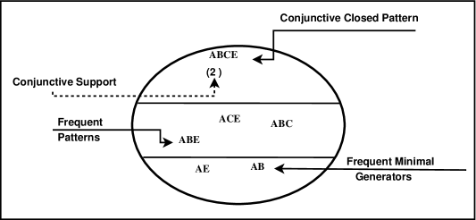
Figure 2.1: Characterization of a Conjunctive Equivalence Class.

At this level, we have presented the basic notions related to itemset’s extraction and to condensed representations.

2.4 Conclusion

Different approaches, derived from Formal Concept Analysis (FCA), were proposed in order to reduce the size of the set of frequent itemsets. In addition, correlated pattern mining constitutes an interesting alternative to get more informative patterns with a manageable size and a high quality returned knowledge.
The next chapter will be dedicated to the presentation, going from the general to the more specific, of the state of the art approaches related to correlated patterns mining. A Comparative study of these approaches will be also conducted.

Chapter 3 Correlated Patterns Mining: Review of the Literature

3.1 Introduction

In this chapter, we focus on presenting an overview of the literature approaches, which are related to our topic of mining correlated patterns. Our study goes from general to more specific. In this respect, we present in Section 3.2 the approaches related to constraint-based data mining, we deal with the two kinds of constraints. Then, in Section 3.3, we specially concentrate on correlated pattern mining. We start by introducing the most common correlation measures, then we join with the state of the art of rare correlated patterns mining followed by frequent correlated patterns mining approaches. A synthetic summary of the studied approaches is proposed in Section 3.4. The chapter is concluded in Section 3.5.

3.2 Constraint-based Itemset Mining

Within a process of pattern extraction, it is more difficult to localize the set of patterns fulfilling a set of constraints of different natures than to extract theories associated to a conjunction of constraints of the same nature [Bonchi and Lucchese, 2006]. Indeed, the opposite nature of the constraints makes that the reduction strategies are applicable to only a part of the constraints and not to all the constraints. Therefore, the extraction process will be more complicated and more expensive in terms of execution costs and memory greediness.

Many approaches have paid attention to the extraction of interesting patterns under constraints [Boulicaut and Jeudy, 2010]. One of the first algorithms belonging to this context is DualMiner [Bucila et al., 2003]. The latter allows the reduction of the search space while considering both of the monotonic and the anti-monotonic constraints. However, as highlighted by [Boley and Gärtner, 2009], DualMiner suffers from a main drawback related to the high cost of constraints evaluation.

In [Lee et al., 2006a], the authors have proposed an approach of pattern extraction under constraints. The ExAMiner algorithm [Bonchi et al., 2005] was also proposed in order to mine frequent patterns under monotonic constraints. It is important to mention that the effective reduction strategy adopted by ExAMiner could not be of use in the case of the monotonic constraint of rarity that we treat in this work, since this latter is sensitive to the changes in the transactions of the extraction context.

Many other works have also emerged. We cite for example, the VST algorithm [De Raedt et al., 2002] which allows the extraction of all the strings satisfying the set of monotonic and anti-monotonic constraints. Later, the FAVST algorithm [Lee and De Raedt, 2004] was introduced in order to improve the performance of the VST algorithm by reducing the number of scans of the database. Other approaches, belonging to this framework, have also been proposed such as the DPC-COFI algorithm and the BifoldLeap algorithm [El-Hajj et al., 2005]. The strategy of these approaches consists in extracting the maximal frequent itemsets which fulfill all of the constraints and from which the set of all the frequent valid itemsets will be derived.

In [Guns et al., 2013], the authors proposed the MiningZinc framework dedicated to constraint programming for itemset mining. The constraints are defined, within the MiningZinc system, in a declarative way close to mathematical notations. The solved tasks within the proposed system concerns closed frequent itemset mining, cost-based itemset mining, high utility itemset mining and discriminative patterns mining. In a more generic way, in [Guns, 2016], the author presented a generic overview of methods devoted to bridge the gap between the two fields of constraint-based itemset mining and constraint programming.

3.3 Correlated Pattern Mining

This section is dedicated to the study of the correlated pattern mining. First, we start by introducing the commonly used correlation measures, presenting their properties and comparing them.

3.3.1 Correlation Measures

The integration of the correlation measures within the mining process allows to reduce the number of the extracted patterns while improving the quality of the retrieved knowledge. The quality is expressed by the degree of correlation between the items composing the result itemsets. To achieve this goal, different correlation measures were proposed in the literature, we start with the bond measure.

3.3.1.1 The bond measure

The bond measure [Omiecinski, 2003] is mathematically equivalent to Coherence [Lee et al., 2003], Tanimoto-coefficient [Tanimoto, 1958], and Jaccard. In [Ben Younes et al., 2010], the authors propose a new expression of bond in Definition 22.

Definition 22

The bond measure
The bond measure of a non-empty pattern $I$ $\subseteq$ $\mathcal{I}$ is defined as follows:

$\textit{bond}\textsc{(}\textit{I}\textsc{)}=\frac{\displaystyle\textit{Supp}\textsc{(}\wedge\textit{I}\textsc{)}}{\displaystyle\textit{Supp}\textsc{(}\vee\textit{I}\textsc{)}}$

This measure conveys the information about the correlation of a pattern $I$ by computing the ratio between the number of co-occurrences of its items and the cardinality of its universe, which is equal to the transaction set containing a non-empty subset of $I$. It is worth mentioning that, in the previous works dedicated to this measure, the disjunctive support has never been used to express it.

The use of the disjunctive support allows to reformulate the expression of the bond measure in order to bring out some pruning conditions for the extraction of the patterns fulfilling this measure. Indeed, as shown later, the bond measure fulfills several properties that offer interesting pruning strategies allowing to reduce the number of generated pattern during the extraction process. Note that the value of the bond measure of the empty set is undefined since its disjunctive support is equal to $0$. However, this value is positive since $\lim_{I\mapsto\emptyset}$ bond (I) = $\frac{\displaystyle|\mathcal{T}|}{\displaystyle 0}$ = $+\infty$. As a result, the empty set will be considered as a correlated pattern for any minimal threshold of the bond correlation measure.

It has been proved, in [Ben Younes et al., 2010], that the bond measure fulfills other interesting properties. In fact, bond is: ($i$) Symmetric since we have $\forall$ $I$, $J$ $\subseteq$ $\mathcal{I}$, bond($IJ$) = bond($JI$); ($ii$) descriptive i.e. is not influenced by the variation of the number of the transactions of the extraction context.

In addition, it has been shown in [Wu et al., 2010] that it is desirable to select a descriptive measure which is not influenced by the number of transactions that contain none of pattern items. The symmetric property fulfilled by the bond measure makes it possible not to treat all the combinations induced by the precedence order of items within a given pattern. Noteworthily, the anti-monotony property, fulfilled by the bond measure as proven in [Omiecinski, 2003], is of interest. Indeed, all the subsets of a correlated pattern are also necessarily correlated. Then, we can deduce that any pattern having at least one uncorrelated proper subset is necessarily uncorrelated. It will thus be pruned without computing the value of its bond measure. In the next definition, we introduce the relationship between the bond measure and the cross-support property.

Definition 23

Cross-support property of the bond measure [Xiong et al., 2006]
Thanks to the cross-support property, having a minimal threshold minbond and an itemset $I$ $\subseteq$ $\mathcal{I}$, if $\exists$ $x$ and $y$ $\in$ $I$ such as $\frac{\displaystyle\textit{Supp}\textsc{(}\wedge x\textsc{)}}{\displaystyle\textit{Supp}\textsc{(}\wedge y\textsc{)}}<\textit{minbond}$ then $I$ is not correlated since bond($I$) < minbond;

We continue, in what follows, with the presentation of the all-confidence measure.

3.3.1.2 The all-confidence measure

The all-confidence measure [Omiecinski, 2003] is defined as follows:

Definition 24

The all-confidence measure
The all-confidence measure [Omiecinski, 2003] is defined for any non-empty set $I$ $\subseteq$ $\mathcal{I}$ as follows:

all-conf($I$) = $\displaystyle\frac{\displaystyle\textit{Supp}\textsc{(}\wedge I\textsc{)}}{\displaystyle\textit{max}\{\textit{Supp}\textsc{(}\wedge i\textsc{)}|i\in I\}}$

All-confidence conserves the anti-monotonic property [Omiecinski, 2003] as well as the cross-support property [Xiong et al., 2006].

Example 10

Let us consider the extraction context given by Table 2.1 (cf. page 2.1) . For a minimal threshold of all-confidence equal to 0.4. We have all-confidence(ABCE) =

$$\frac{\displaystyle\textit{Supp}\textsc{(}\wedge\texttt{ABCE}\textsc{)}}{\displaystyle\textit{max}\{\textit{Supp}\textsc{(}\wedge\texttt{A}\textsc{)},\textit{Supp}\textsc{(}\wedge\texttt{B}\textsc{)},\textit{Supp}\textsc{(}\wedge\texttt{C}\textsc{)},\textit{Supp}\textsc{(}\wedge\texttt{E}\textsc{)}\}}$$

=

$$\frac{\displaystyle 2}{\displaystyle\textit{max}\{3,4\}}$$

= 0.50. The ABCE itemset is correlated according to the all-confidence measure. All the direct subsets of ABCE are also correlated. We have all-confidence(ABE) = all-confidence(ACE) = $\displaystyle\frac{\displaystyle 2}{\displaystyle 4}$ = 0.50, all-confidence(BCE) = $\displaystyle\frac{\displaystyle 3}{\displaystyle 4}$ = 0.75.

For the itemset AD, we have $\displaystyle\frac{\displaystyle\textit{Supp}\textsc{(}\wedge\textsl{D}\textsc{)}}{\displaystyle\textit{Supp}\textsc{(}\wedge\textsl{A}\textsc{)}}$ $=$ $\displaystyle\frac{\displaystyle 1}{\displaystyle 3}$ = 0.33 $<$ 0.4 and we have all-confidence(AD) = $\displaystyle\frac{\displaystyle 1}{\displaystyle 3}$ = 0.33. The AD itemset does not fulfill the cross-support property, thus it is a non-correlated itemset. This example illustrates the conservation of the anti-monotonicity and the cross-support properties of the all-confidence measure.

We continue in what follows with the hyper-confidence measure.

3.3.1.3 The hyper-confidence measure

The hyper-confidence measure denoted by h-conf of an itemset $I$ $\subseteq$ $\mathcal{I}$ is defined as follows.

Definition 25

The hyper-confidence measure
The hyper-confidence measure of an itemset $I$ $=$ $\{$$i_{1}$, $i_{2}$, $\ldots$, $i_{m}$$\}$ is equal to:

h-conf($X$)=min$\{$Conf( $i_{1}$ $\Rightarrow$ $i_{2}$, $i_{3}$, $\ldots$, $i_{m}$ ), $\ldots$, Conf($i_{m}$ $\Rightarrow$ $i_{1}$, $i_{2}$, $\ldots$, $i_{m-1}$ )$\}$,

where Conf stands for the Confidence measure associated to association rules.

The hyper-confidence measure is equivalent to the all-confidence measure, it thus fulfills the anti-monotonicity and the cross-support properties.

We continue in what follows with the any-confidence measure.

3.3.1.4 The any-confidence measure

This measure is defined, for any non empty set $I$ $\subseteq$ $\mathcal{I}$ as follows:

Definition 26

The any-confidence measure

any-conf($I$) = $\displaystyle\frac{\displaystyle\textit{Supp}\textsc{(}\wedge I\textsc{)}}{\displaystyle\textit{min}\{\textit{Supp}\textsc{(}\wedge i\textsc{)}|i\in I\}}$

The any-confidence measure [Omiecinski, 2003] does not preserve nor the anti-monotonicity neither the cross-support properties.

Example 11

Let us consider the extraction context given by Table 2.1. For a minimal correlation threshold equal to 0.80. The any-confidence value of AB is equal to, any-confidence(AB) = $\displaystyle\frac{\displaystyle\textit{Supp}\textsc{(}\wedge\texttt{AB}\textsc{)}}{\displaystyle\textit{min}\{\textit{Supp}\textsc{(}\wedge\texttt{A}\textsc{)},\textit{Supp}\textsc{(}\wedge\texttt{B}\textsc{)}\}}$ = $\displaystyle\frac{\displaystyle 2}{\displaystyle\textit{min}\{3,4\}}$ = 0.66. AB do not fulfill the minimal threshold of correlation, thus it is a non-correlated itemset according to the any-confidence measure. Whereas, the AD itemset is correlated and its correlation value is equal to 1. We also have, $\displaystyle\frac{\displaystyle\textit{Supp}\textsc{(}\wedge\textsl{A}\textsc{)}}{\displaystyle\textit{Supp}\textsc{(}\wedge\textsl{C}\textsc{)}}$ $=$ $\displaystyle\frac{\displaystyle 3}{\displaystyle 4}$ = 0.75 $<$ 0.80, however, any-confidence(AD) $=$ 1 $>$ 0.80. This example illustrates the non preservation of the anti-monotonicity as well as the cross-support properties.

We present in what follows the $\chi^{2}$ Coefficient.

3.3.1.5 The $\chi^{2}$ Coefficient

The $\chi^{2}$ coefficient is defined as follows :

Definition 27

The $\chi^{2}$ Coefficient [Brin et al., 1997]
The $\chi^{2}$ coefficient of an itemset $Z$ $=$ $xy$, with $x$ and $y$ $\in$ $\mathcal{I}$, is defined as follows:

$\chi^{2}$($Z$) $=$ $|\mathcal{T}|$ $\times$ $\frac{\displaystyle\textsc{(}\textit{Supp}\textsc{(}\wedge xy\textsc{)}-\textit{Supp}\textsc{(}\wedge x\textsc{)}\times\textit{Supp}\textsc{(}\wedge y\textsc{)}\textsc{)}^{2}}{\displaystyle\textit{Supp}\textsc{(}\wedge x\textsc{)}\times\textit{Supp}\textsc{(}\wedge y\textsc{)}\times\textsc{(}1-\textit{Supp}\textsc{(}\wedge x\textsc{)}\textsc{)}\times\textsc{(}1-\textit{Supp}\textsc{(}\wedge y\textsc{)}\textsc{)}}$

Some relevant properties of the $\chi^{2}$ coefficient are given by the following proposition.

Proposition 4

The $\chi^{2}$ coefficient is a statistic and symmetric measure [Brin et al., 1997].

Other correlation measures are also of use in the literature, we mention for example the cosine measure, the lift measure [Brin et al., 1997], the $\phi$ coefficient also named the Pearson coefficient [Xiong et al., 2004].

3.3.1.6 Synthesis

We recapitulate the different properties of the presented measures in Table 3.1. The “$\checkmark$” symbol indicates that the measure fulfills the property.

In our previous study, we specifically focused on correlation measures which are most used in correlated patterns mining. Withal, the cosine and the kulczynski measures were not studied since these two measures are rarely used on correlated patterns mining due to the non conservation of the anti-monotonicity property [Wu et al., 2010]. The lift measure is used within the association rule evaluation.

Measure	Independence of $|\mathcal{T}|$	Symmetry	Anti-monotonicity	Cross-support
bond	$\checkmark$	$\checkmark$	$\checkmark$	$\checkmark$
any-confidence	$\checkmark$	$\checkmark$
all-confidence	$\checkmark$	$\checkmark$	$\checkmark$	$\checkmark$
hyper-confidence	$\checkmark$	$\checkmark$	$\checkmark$	$\checkmark$
$\chi^{2}$		$\checkmark$

Table 3.1: Summary of the properties of the studied correlation measures and coefficients.

We conclude, according to this overview, that the most interesting measures are bond and all-confidence. This is justified by the fact that these two measures fulfilled the pertinent properties of anti-monotonicity and cross-support.

We present, in what follows, the state of the art approaches dealing with correlated patterns mining. We precisely start with rare correlated pattern mining.

3.3.2 Rare Correlated Patterns Mining

Various approaches devoted to the extraction of correlated patterns under constraints have been proposed. However, the recuperation of all the patterns that are both highly correlated and infrequent is based on the naive idea to extract the set of all frequent patterns for a very low threshold minsupp and then to filter out these patterns by a measure of correlation.

Another idea is to extract the whole set of the correlated patterns without any integration of the rarity constraint. The obtained set contains obviously all the frequent correlated as well as the rare correlated patterns. It is relevant to note that the application of these two ideas is very expensive in execution time and in memory consumption due to the explosion of the number of candidates to be evaluated.

The approach proposed in [Cohen et al., 2000] is based on the previous principle. This approach allows to extract the items’s pairs correlated according to the Similarity measure but without computing their support. In fact, the Similarity measure allows to evaluate the similarity between two items and corresponds to the quotient of the number of the simultaneous appearance divided by the number of the complementary appearance. Consequently, the Similarity measure is semantically equivalent to the bond measure. However, any analysis of this measure have been conducted.
In fact, this approach proposes to assign to each item a signature composed by the identifier list of the transactions to which the item belongs. Then, the Similarity is computed and it corresponds to the number of the intersections of their signatures divided by the union of their signatures. We conclude that the frequency constraint was not integrated in order to recuperate the highly correlated itemsets with a weak support. From these patterns, the association rules with a high confidence and a weak support are generated.

In this same context, we mention the DiscoverMPatterns algorithm [Ma and Hellerstein, 2001]. In fact, this latter is devoted to the extraction of the correlated patterns based on the all-confidence measure. Nevertheless, a first version of the approach was dedicated to the extraction of all the correlated patterns without any restriction of the support value in order to specifically get the rare correlated itemsets. Then, within the second version of the approach, the minimum support threshold constraint was integrated. Consequently, this constraint integration allows to extract the frequent correlated patterns.

Another principle of the resolution of the rare correlated patterns extraction consists in extracting all the frequent patterns for a very weak minimal support threshold. Evidently, the obtained set contains a subset of the infrequent correlated patterns. Xiong et al. relied on this idea to introduce the Hyper-CliqueMiner algorithm [Xiong et al., 2006]. The output of this algorithm is the set of frequent correlated patterns for a very low minsupp value. It is to note, that the good performances of this algorithm are justified by the use of the anti-monotonic property of the correlation measure as well as the cross-support property which allows to reduce significantly the evaluated candidates and thus to reduce the time needed.

The approach proposed in [Sandler and Thomo, 2010] stands also within this principle. This approach allows to extract the frequent and frequently correlated 2-itemsets. It is judged as a naive approach that is based on the extraction of all the solution set for a very low minsupp values. Then, a post processing is performed in order to maintain only the high correlated itemsets. The FT-Miner algorithm [Hu and Li, 2009] outputs the correlated infrequent itemsets according to the N-Confidence semantically equivalent to all-Confidence. The all-Confidence measure was also treated in the Partition algorithm [Omiecinski, 2003], which allows to extract the correlated patterns according to both all-Confidence and bond measures. The choice of the measure to be considered depends on the user’s input preferences.

The approach proposed in [Okubo et al., 2010] also belongs to the same trend of approaches dealing with correlated infrequent itemsets. Indeed, it is based on the principle that the patterns which are weakly correlated according to the bond correlation measure are generally rare in the extraction context. The expressed constraint corresponds to a restriction of the maximum correlation value. This is a monotonic constraint since it corresponds to the opposite of the anti-monotonic constraint of minimal correlation. In order to get rid from rare patterns that represent exceptions, and they are not informative, a minimal frequency constraint was also integrated. The idea consists then in extracting the top$-N$ rare patterns which are the most informative ones.

The problem of integrating constraints during the process of correlated pattern mining was also studied in the works, respectively, proposed in [Brin et al., 1997] and in [Grahne et al., 2000]. These approaches deal with constrained correlated pattern mining, they rely on the $\chi^{2}$ correlation coefficient. They exploit the various pruning opportunities offered by these constraints and benefit from the selective power of each type of constraints. However, the coefficient $\chi^{2}$ does not fulfill the anti-monotonic constraint as does the bond measure. Besides, these approaches are limited to the extraction of a small subset which is composed only by minimal valid patterns i.e. the minimal patterns which fulfill all of the imposed constraints. Furthermore, the authors do not propose any concise representation of the extracted correlated patterns.

Also, in [Surana et al., 2010], a study of different properties of interesting measures was conducted in order to suggest a set of the most adequate properties to consider while mining rare associations rules.

It is deduced that for all these approaches, the monotonic constraint of rarity was never included within the mining process in order to retrieve all the rare highly correlated patterns.

3.3.3 Frequent Correlated Patterns Mining

In [Lee et al., 2003], the authors proposed the CoMine approach which is dedicated to the extraction of frequent correlated patterns according to the all-confidence and to the bond measures. We distinguish two different versions of the CoMine approach. The first version treats the bond measure while the second treats the all-Confidence measure. CoMine also constitute the core of the I-IsCoMine-AP and I-IsCoMine-CT algorithms [SHEN et al., 2011].

Also, the bond measure was studied in [Le Bras et al., 2011], the authors proposed an apriori-like algorithm for mining classification rules. Moreover, the authors in [Segond and Borgelt, 2011] proposed a generic approach for frequent correlated pattern mining. Indeed, the bond correlation measure and eleven other correlation measures were used. All of them fulfill the anti-monotonicity property. Correlated patterns mining was then shown to be more complex and more informative than frequent pattern mining [Segond and Borgelt, 2011].

Many other works have also emerged. In [Wu et al., 2010], the authors provide a unified definition of existing null-invariant correlation measures and propose the GAMiner approach allowing the extraction of frequent high correlated patterns according to the Cosine and to the Kulczynsky measures. In this same context, the NICOMiner algorithm was also proposed in [Kim et al., 2011] and it allows the extraction of correlated patterns according to the Cosine measure. We highlight that the Cosine measure has the specificity of being not monotonic neither anti-monotonic.

In this same context, we also cite the Atheris approach [Soulet et al., 2011] which allows the extraction of condensed representation of correlated patterns according to user’s preferences. In [Barsky et al., 2012], the authors introduced the concept of flipping correlation patterns according to the Kulczynsky measure. However, the Kulczynsky measure does not fulfill the interesting anti-monotonic property as the bond measure.

The all-confidence measure was handled within the work proposed in [Karim et al., 2012]. The approach outputs the correlated patterns (also called the associated patterns), the non correlated patterns (also called the independent patterns). Also, in [Kiran and Kitsuregawa, 2013] the authors propose a method to extract all-confidence frequent correlated patterns and they also discuss the impact of fixing the minsupp threshold value over the quality of the obtained itemsets and propose to fix a minimal correlation threshold for each item.

In the next subsection, we study the approaches of extracting the condensed representations of frequent correlated patterns.

3.3.4 Condensed Representations of Correlated Patterns Mining

The problem of mining concise representations of correlated patterns was not widely studied in the literature. We mention the Ccmine [Kim et al., 2004] approach of mining closed correlated patterns according to the all-confidence measure which constitute a condensed representation of frequent correlated patterns. We also precise that the authors in [Ben Younes et al., 2010] proposed the CCPR-Miner algorithm allowing the extraction of closed frequent correlated patterns according to the bond measure.

In this context, we also cite the Jim approach [Segond and Borgelt, 2011]. In fact, Jim allows to extract the closed correlated frequent patterns which constitute a perfect cover of the whole set of frequent correlated patterns. The choice of the considered correlation measure is fixed by the user’s parameters within the Jim approach.

In fact, the Jim approach is, on the one hand the most efficient state of the art approach extracting condensed representation of frequent correlated patterns according to the bond measure. On the other hand, Jim is the unique approach which dealt with the same kind of patterns as we treat in our mining approach, that we present in the following chapters. In this sense, in our experimental study, we will focus on comparing our mining approach by the Jim approach.

3.4 Discussion

Based on the previous review of the literature, we conclude that most of the approaches dealt with the bond and the all-confidence measures. These latter fulfill the interesting anti-monotonic property, that allows to reduce the search space by early pruning irrelevant candidates. Therefore, the frequent correlated set of patterns results from the conjunction of both constraints of the same type: the correlation and the frequency.

In fact, the recuperation of all the patterns that are both highly correlated and infrequent is based on the naive idea to extract the set of all frequent patterns for a very low threshold minsupp and then to filter out these patterns by a measure of correlation. Another resolution strategy consists in extracting the whole set of the correlated patterns without any integration of the rarity constraint. Then, a post-processing is performed in order to uniquely retrieve the rare correlated itemsets.

In other words, the monotonic constraint of rarity was never integrated within the mining process and thus the exploration of the search space of candidates that does not fulfill the rarity constraint is obviously barren. In addition, another problem is related to the high consuming of the memory and the CPU resources due to the combinatorial explosion of the number of candidates depending on the size of the mined dataset. We highlight, that Jim [Segond and Borgelt, 2011] is the unique approach that dealt with different anti-monotonic correlation measures. However, Jim is limited to frequent correlated patterns and do not consider the rare correlated ones.

Table 3.2 recapitulates the characteristics of the different visited approaches. This table summarizes the following properties:

1. The correlation measure: This property describes the considered correlation measure.

2. The kind of the extracted patterns: This property describes the kind of patterns outputted by the mining algorithm

3. The nature of constraints: This property describes the nature of the constraints included within the algorithm: anti-monotonic or monotonic.

To the best of our knowledge, no previous work was dedicated to the extraction of concise representations of patterns under the conjunction of constraints of distinct types. This problem is then a challenging task in data mining, which strengthens our motivation for the treatment of this problematic. Therefore, the work proposed in this thesis is the first one that puts the focus on mining concise representations of both frequent and rare correlated patterns according to the anti-monotonic bond measure.

Extraction	Correlation	Kind of the extracted	Nature of
Algorithm	Measure	Patterns	Constraints
The approach of	bond	correlated	anti-monotonic
[Cohen et al., 2000]		2-itemsets
DiscoverMPattern	all-confidence	all the correlated	anti-monotonic
[Ma and Hellerstein, 2001]		itemsets
Partition	all-confidence	all the correlated	anti-monotonic
[Omiecinski, 2003]	bond	itemsets
CoMine($\alpha$)	all-confidence	correlated frequent	anti-monotonic
[Lee et al., 2003]
CoMine($\gamma$)	bond	correlated frequent	anti-monotonic
[Lee et al., 2003]
CCMine	all-confidence	closed	anti-monotonic
[Kim et al., 2004]		frequent correlated
HypercliqueMiner	h-confidence	correlated frequent	anti-monotonic
[Xiong et al., 2006]		and a subset of rare
		correlated itemsets
The approach of	all-confidence	correlated frequent
[Sandler and Thomo, 2010]		and a subset of rare	anti-monotonic
		correlated itemsets
The approach of	bond	weakly correlated	monotonic
[Okubo et al., 2010]
CCPR_Miner	bond	closed	anti-monotonic
[Ben Younes et al., 2010]		frequent correlated
Jim	Eleven different	closed	anti-monotonic
[Segond and Borgelt, 2011]	anti-monotonic	frequent correlated
	measures	and frequent correlated

Table 3.2: Comparison between the correlated patterns mining approaches.

3.5 Conclusion

In this chapter, we proposed an overview of the state of the art approaches dealing with correlated patterns mining preceded by a presentation of the different correlation measures. We deduced that, there is no previous work that dealt with both frequent correlated as well as rare correlated patterns according to a specified correlation metric. Thus, motivated by this issue, we propose in this thesis to benefit from the knowledge returned from both frequent correlated as well as rare correlated patterns according to the bond measure. To tackle this challenging task, we propose in the next chapter the characterization of both frequent correlated patterns, rare correlated patterns and their associated concise representations.

Part II Condensed Representations of Correlated Patterns

Chapter 4 Condensed Representations of Correlated Patterns

4.1 Introduction

The main moan that can be related to frequent pattern mining approaches stands in the fact that the latter do not offer the information concerning the correlation degree among the items in the extraction context. This stands behind our motivation to provide to the user the key information about the correlation between items as well as the frequency of their occurrence. This aim is reachable thanks to the integration of the correlation measures within the mining process.

The correlation measure, that we treat throughout this thesis, is bond. Our motivations behind the choice of this measure is explicitly described in Section 4.2. In Section 4.3, we focus on the correlated patterns associated to the bond measure, we characterize this set of patterns. Section 4.4 is devoted to the presentation of the closure operator associated to bond. We introduce the associated exact condensed representations in Section 4.5 and in Section 4.6. Section 4.7 concludes the chapter.

4.2 Motivations behind our choice of the bond measure

Based on the study of the state of the art approaches proposed in the previous chapter, we find that the almost of the existing approaches are dealing with the bond and the all-confidence measures. The bond measure fulfills the anti-monotony property which is an interesting property. Indeed, the latter reduce the search space when pruning the non potential candidates, therefore optimizing the extraction time as well as the memory consumption.

It has been proved in the literature that the bond measure presents many interesting properties. In fact, the bond measure is:

1. symmetric since $\forall$ $I$, $J$ $\subseteq$ $\mathcal{I}$, bond($IJ$) = bond($JI$);

2. descriptive since it is not influenced by the number of transactions that contain none of the items composing the pattern;

3. fulfills the cross-support property [Xiong et al., 2006]. Thanks to this property, given a minimal threshold minbond and an itemset $I$ $\subseteq$ $\mathcal{I}$, if $\exists$ $x$ and $y$ $\in$ $I$ such as $\frac{\displaystyle\textit{Supp}\textsc{(}\wedge x\textsc{)}}{\displaystyle\textit{Supp}\textsc{(}\wedge y\textsc{)}}<\textit{minbond}$ then $I$ is not correlated since bond($I$) $<$ minbond;

4. induces an anti-monotonic constraint for a fixed minimal threshold minbond. In fact, $\forall$ $I$, $I_{1}$ $\subseteq$ $\mathcal{I}$, if $I_{1}$ $\subseteq$ $I$, then bond($I_{1}$) $\geq$ bond($I$). Therefore, the set $\mathcal{CP}$ of correlated patterns forms an order ideal. Indeed, all the subsets of a correlated pattern are necessarily correlated ones.

We present in the following an interesting relation between the value of the bond measure and the conjunctive and disjunctive supports values for each couple of two patterns $I$ and $I_{1}$ such as $I$ $\subseteq$ $I_{1}$ [Ben Younes et al., 2010].

Proposition 5

Let $I$, $I_{1}$ $\subseteq$ $\mathcal{I}$ and $I$ $\subseteq$ $I_{1}$. If bond($I$) = bond($I_{1}$), then Supp($\wedge I$) = Supp($\wedge I_{1}$) and Supp($\vee I$) = Supp($\vee I_{1}$).

According to the previous proposal, if bond($I$) = bond($I_{1}$), then Supp($\neg I$) = Supp($\neg I_{1}$). In fact, both $I$ and $I_{1}$ have the same conjunctive support and, according to the Morgan law, we build the following relation between the disjunctive and the negative supports of a pattern: Supp($\neg I$) = $|\mathcal{T}|$ - Supp($\vee I$). On the other hand, if bond($I$) $\neq$ bond($I_{1}$), then Supp($\wedge I$) $\neq$ Supp($\wedge I_{1}$) or Supp($\vee I$) $\neq$ Supp($\vee I_{1}$) (i.e. one of the two supports is different or both).

In this context, we propose to study the bond correlation measure in an integrated mining process aiming to extract both frequent and rare correlated patterns as well as their associated condensed representations. In this regard, we present in the next section the specification of the frequent correlated patterns as well as the rare correlated patterns according to the bond measure.

4.3 Characterization of the Correlated patterns according to the bond measure

4.3.1 Definitions and Properties

The bond measure [Omiecinski, 2003] is mathematically equivalent to Coherence [Lee et al., 2003], Tanimoto coefficient [Tanimoto, 1958], and Jaccard [Jaccard, 1901]. It was redefined in [Ben Younes et al., 2010] as follows:

Definition 28

The bond measure
The bond measure of a non-empty pattern $I\subseteq\mathcal{I}$ is defined as follows:

$\textit{bond}\textsc{(}\textit{I}\textsc{)}=\frac{\displaystyle\textit{Supp}\textsc{(}\wedge\textit{I}\textsc{)}}{\displaystyle\textit{Supp}\textsc{(}\vee\textit{I}\textsc{)}}$

The bond measure takes its values within the interval $[0,1]$. While considering the universe of a pattern $\mathcal{I}$ [Lee et al., 2003], i.e., the set of transactions containing a non empty subset of $I$, the bond measure represents the simultaneous occurrence rate of the items of the pattern $I$ in its universe. Thus, the higher the items of the pattern are dispersed in its universe, (i.e. weakly correlated), the lower the value of the bond measure is, as Supp($\wedge I$) is smaller than Supp($\vee I$). Inversely, the more the items of $I$ are dependent from each other, (i.e. strongly correlated), the higher the value of the bond measure is, since Supp($\wedge I$) would be closer to Supp($\vee I$).

The set of correlated patterns associated to the bond measure is defined as follows.

Definition 29

Correlated patterns
Considering a correlation threshold minbond, the set of correlated patterns, denoted $\mathcal{CP}$, is equal to: $\mathcal{CP}$ = $\{I$ $\subseteq\mathcal{I}|$ bond($I$) $\geq$ minbond$\}$.

Example 12

Let us consider the dataset given by Table 2.1. For minbond = 0.5, we have bond($AB$) = $\displaystyle\frac{2}{5}$ = 0.4 $<$ 0.5. The itemset $AB$ is then not a correlated one. Whereas, since bond($BCE$) = $\displaystyle\frac{3}{5}$ = 0.6 $\geq$ 0.5, the itemset $BCE$ is a correlated one.

In the following, we define the set composed by the maximal correlated patterns as follows:

Definition 30

Maximal correlated patterns
The set of maximal correlated patterns constitutes the positive border of correlated patterns and is composed by correlated patterns having no correlated proper superset. This set is defined as: $\mathcal{M}ax$$\mathcal{CP}$ = $\{$$I$ $\in$ $\mathcal{CP}$$\mid$ $\forall$ $I_{1}$ $\supset$ $I$: $I_{1}$ $\notin$ $\mathcal{CP}$$\}$, or equivalently: $\mathcal{M}ax$$\mathcal{CP}$ = $\{$$I$ $\in$ $\mathcal{CP}$$\mid$ $\forall$ $I_{1}$ $\supset$ $I$: bond($I_{1}$) $<$ minbond$\}$.

Example 13

Consider the extraction context sketched by Table 2.1 (Page 2.1). For minbond = 0.2, we have $\mathcal{M}ax$$\mathcal{CP}$ = $\{$$ACD$, $ABCE$$\}$.

As far as we integrate the frequency constraint with the correlation constraint, we can distinguish between two sets of correlated patterns, which are the "Frequent correlated patterns" set and the "Rare correlated patterns" set. These two distinct sets will be characterized separately in the remainder.

4.3.2 Frequent Correlated Patterns

Definition 31

The set of frequent correlated patterns
Considering the support threshold minsupp and the correlation threshold minbond, the set of frequent correlated patterns, denoted $\mathcal{FCP}$, is equal to: $\mathcal{FCP}$ = $\{$$I$ $\subseteq$ $\mathcal{I}$ $|$ Supp($\wedge I$) $\geq$ minsupp and bond($I$) $\geq$ minbond$\}$.

In fact, the $\mathcal{FCP}$ set is composed by the patterns fulfilling at the same time the correlation and the frequency constraints. A pattern is said to be “Frequent Correlated” if its support exceeds the minimal frequency threshold minsupp and its correlation value also exceeds the minimal correlation threshold minbond. The $\mathcal{FCP}$ set corresponds to the conjunction of two anti-monotonic constraints of correlation and of frequency. Thus, it induces an order ideal on the itmeset lattice.

Example 14

Consider the extraction context sketched by Table 2.1 (Page 2.1). For minsupp = 4 and minbond = 0.2, the $\mathcal{FCP}$ set consists of the following patterns where each triplet represents the pattern, its conjunctive support value and its bond value: $\mathcal{FCP}$ = $\{$($B$, 4, $\displaystyle\frac{4}{4}$), ($C$, 4, $\displaystyle\frac{4}{4}$), ($E$, 4, $\displaystyle\frac{4}{4}$), ($BE$, 4, $\displaystyle\frac{4}{4}$)$\}$.

4.3.3 Rare Correlated Patterns

The set of rare correlated patterns associated to the bond measure is defined as follows.

Definition 32

The set of rare correlated patterns
Considering the support threshold minsupp and the correlation threshold minbond, the set of rare correlated patterns, denoted $\mathcal{RCP}$, is equal to: $\mathcal{RCP}$ = $\{I$ $\subseteq$ $\mathcal{I}$ $|$ Supp($\wedge I$) $<$ minsupp and bond($I$) $\geq$ minbond$\}$.

Example 15

Consider the extraction context sketched by Table 2.1 (Page 2.1). For minsupp = 4 and minbond = 0.2, the set $\mathcal{RCP}$ consists of the following patterns where each triplet represents the pattern, its conjunctive support value and its bond value: $\mathcal{RCP}$ = $\{$($A$, 3, $\displaystyle\frac{3}{3}$), ($D$, 1, $\displaystyle\frac{1}{1}$), ($AB$, 2, $\displaystyle\frac{2}{5}$), ($AC$, 3, $\displaystyle\frac{3}{4}$), ($AD$, 1, $\displaystyle\frac{1}{3}$), ($AE$, 2, $\displaystyle\frac{2}{5}$), ($BC$, 3, $\displaystyle\frac{3}{5}$), ($CD$, 1, $\displaystyle\frac{1}{4}$), ($CE$, 3, $\displaystyle\frac{3}{5}$), ($ABC$, 2, $\displaystyle\frac{2}{5}$), ($ABE$, 2, $\displaystyle\frac{2}{5}$), ($ACD$, 1, $\displaystyle\frac{1}{4}$), ($ACE$, 2, $\displaystyle\frac{2}{5}$), ($BCE$, 3, $\displaystyle\frac{3}{5}$), ($ABCE$, 2, $\displaystyle\frac{2}{5}$)$\}$. This associated $\mathcal{RCP}$ set as well as the $\mathcal{FCP}$ set of the previous example are depicted by Figure 4.1. The support shown at the top left of each frame represents the conjunctive one. As shown in Figure 4.1, the rare correlated patterns are localized below the border induced by the anti-monotonic constraint of correlation and over the border induced by the monotonic constraint of rarity.

We deduce from Definition 32 that the $\mathcal{RCP}$ set corresponds to the intersection between the set $\mathcal{CP}$ of correlated patterns and the set $\mathcal{RP}$ of rare patterns, i.e., $\mathcal{RCP}$ = $\mathcal{CP}$ $\cap$ $\mathcal{RP}$. The following proposition derives from this result.

Proposition 6

Let $I$ $\in$ $\mathcal{RCP}$. We have:

• Based on the order ideal of the set $\mathcal{CP}$ of correlated patterns, we have $\forall$ $I_{1}$ $\subseteq$ $I$: $I_{1}$ $\in$ $\mathcal{CP}$

• Based on the order filter of the set $\mathcal{RP}$ of rare patterns, we have $\forall$ $I_{1}$ $\supseteq$ $I$: $I_{1}$ $\in$ $\mathcal{RP}$.

Proof. The proof follows from the properties induced by the constraints of rarity and correlation. The set $\mathcal{RCP}$, whose elements fulfill the constraint “being a rare correlated pattern”, results from the conjunction between two theories corresponding to both constraints of distinct types. So, the set $\mathcal{RCP}$ is neither an order ideal nor an order filter. The search space of this set is delimited by: (i) The maximal correlated elements which are also rare, i.e. the rare patterns among the set $\mathcal{M}$$ax$$\mathcal{CP}$ of maximal correlated patterns (cf. Definition 30) and; (ii) The minimal rare elements which are correlated, i.e. the correlated patterns among the set $\mathcal{M}$$in$$\mathcal{RP}$ of minimal rare patterns (cf. Definition 5). Therefore, each rare correlated pattern is necessarily included between an element from each set of the two aforementioned sets.

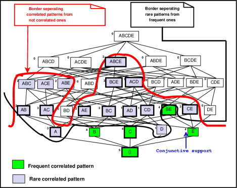
Figure 4.1: Localization of the correlated patterns for minsupp = 4 and minbond = 0.2 according to the extraction context given in Table 2.1.

Therefore, the localization of these elements is more difficult than the localization of theories corresponding to constraints of the same nature. Indeed, the conjunction of anti-monotonic constraints (resp. monotonic) is an anti-monotonic one (resp. monotonic) [Bonchi and Lucchese, 2006]. For example, the constraint "being a correlated frequent pattern" is anti-monotonic, since it results from the conjunction of two anti-monotonic constraints namely, "being a correlated pattern" and "being a frequent pattern". This constraint induces, then, an order ideal on the itemset lattice [Ben Younes et al., 2010]. However, the constraint “being a rare and a not correlated pattern” is monotonic, since it results from the conjunction of two monotonic constraints namely, "being a not correlated pattern” and "being a rare pattern”. This constraint induces, then, an order filter on the itemset lattice.

In order to assess the size of the $\mathcal{RCP}$ set, and given the nature of the two constraints induced by the minimal thresholds of rarity and correlation respectively minsupp and minbond, the size of the $\mathcal{RCP}$ set of rare correlated patterns varies as shown in the following proposition.

Proposition 7

a) Let minsupp₁ and minsupp₂ be two minimal thresholds of conjunctive support and $\mathcal{RCP}_{s1}$ and $\mathcal{RCP}_{s2}$ be the two sets of patterns associated to each threshold for the same value of minbond. We have: if minsupp₁ $\leq$ minsupp₂, then $\mathcal{RCP}_{s1}$ $\subseteq$ $\mathcal{RCP}_{s2}$ and consequently $|\mathcal{RCP}_{s1}|$ $\leq$ $|\mathcal{RCP}_{s2}|$.
b) Let minbond₁ and minbond₂ be two minimal thresholds of bond measure and let $\mathcal{RCP}_{b1}$ and $\mathcal{RCP}_{b2}$ be the two sets of patterns associated to each threshold for the same value of minsupp. We have: if minbond₁ $\leq$ minbond₂, then $\mathcal{RCP}_{b2}$ $\subseteq$ $\mathcal{RCP}_{b1}$, consequently $|\mathcal{RCP}_{b2}|$ $\leq$ $|\mathcal{RCP}_{b1}|$.

Proof. - The proof of a) derives from the fact that for $I$ $\subseteq$ $\mathcal{I}$, if Supp($\wedge I$) $<$ minsupp₁, then Supp($\wedge I$) $<$ minsupp₂. Therefore, $\forall$ $I$ $\in$ $\mathcal{RCP}_{s1}$, $I$ $\in$ $\mathcal{RCP}_{s2}$. As a result, $\mathcal{RCP}_{s1}$ $\subseteq$ $\mathcal{RCP}_{s2}$.
- The proof of b) derives from the fact that for $I$ $\subseteq$ $\mathcal{I}$, if bond($I$) $\geq$ minbond₂, then bond($I$) $\geq$ minbond₁. Therefore, $\forall$ $I$ $\in$ $\mathcal{RCP}_{b2}$, $I$ $\in$ $\mathcal{RCP}_{b1}$. As a result, $\mathcal{RCP}_{b2}$ $\subseteq$ $\mathcal{RCP}_{b1}$.


We can then deduce that the size of the set $\mathcal{RCP}$ is proportional to minsupp and inversely proportional to minbond. However, in the general case, we cannot decide about the size of the set $\mathcal{RCP}$ when both thresholds vary simultaneously. The next section is dedicated to the presentation of the closure operator associated to the bond measure. This operator characterizes the correlated patterns through the induced equivalence classes.

4.4 The $f_{bond}$ closure operator

The $f_{bond}$ closure operator associated to the bond measure is defined as follows [Ben Younes et al., 2010]:

Definition 33

The operator $f_{bond}$

$$\large f_{bond}:\mathcal{P}\textsc{(}\mathcal{I}\textsc{)} \rightarrow \mathcal{P}\textsc{(}\mathcal{I}\textsc{)}$$

$$I \mapsto f_{bond}\textsc{(}I\textsc{)}=I\cup\{i\in\mathcal{I}\setminus I|\ \textit{bond}\textsc{(}I\textsc{)}=\textit{bond}\textsc{(}I\cup\{i\}\textsc{)}\}$$

The operator $f_{bond}$ has been shown to be a closure operator [Ben Younes et al., 2010]. Indeed, it fulfills the extensitivity, the isotony and the idempotency properties [Ganter and Wille, 1999]. The closure of a pattern $I$ by $f_{bond}$, i.e. $f_{bond}\textsc{(}I$), corresponds to the maximal set of items containing $I$ and sharing the same bond value with $I$.

Example 16

Consider the extraction context sketched by Table 2.1 (Page 2.1). For minbond = 0.2, we have bond($AB$) = $\displaystyle\frac{2}{5}$, bond($ABC$) = $\displaystyle\frac{2}{5}$ and bond($ABE$) = $\displaystyle\frac{2}{5}$. Thus, $C$ $\in$ $f_{bond}$($AB$), and $E$ $\in$ $f_{bond}$($AB$). Contrariwise, bond($ABD$) = $\displaystyle\frac{0}{5}$ = 0. Thus, $D$ $\notin$ $f_{bond}$($AB$). Consequently, we have $f_{bond}$($AB$) = $ABCE$.

Let us illustrate the different properties of the $f_{bond}$ closure operator:

1. For the Extensitivity property: we have, for example, $f_{bond}$(CD) = ACD, CD $\subseteq$ $f_{bond}$(CD).

2. For the Isotony property: we have, for example, AB $\supset$ B, $f_{bond}$(AB) = ABCE and $f_{bond}$(B) = BE.

3. For the Idempotency property: we have, the example of the closed itemset ABCE, $f_{bond}$($f_{bond}$(ABCE)) = ABCE.

The closure operator $f_{bond}$ induces an equivalence relation on the power-set of the set of items $\mathcal{I}$, splitting it into disjoint $f_{bond}$ equivalence classes which are formally defined as follows:

Definition 34

Equivalence class associated to the closure operator $f_{bond}$
An equivalence class associated to the $f_{bond}$ closure operator is composed by all the patterns having the same closure by the operator $f_{bond}$.

In each class, all the elements have the same $f_{bond}$ closure and the same value of bond. The minimal patterns of a bond equivalence class are the smallest incomparable members, w.r.t. set inclusion, while the $f_{bond}$ closed pattern is the largest one. These sets are formally defined in the following:

Definition 35

Closed correlated patterns
The set $\mathcal{CCP}$ of closed correlated patterns by $f_{bond}$ is equal to: $\mathcal{CCP}$ = $\{$$I$ $\in$ $\mathcal{CP}$$\mid$ $\nexists$ $I_{1}$ $\supset$ $I$: bond($I$) = bond($I_{1}\textsc{)}\}$, or equivalently: $\mathcal{CCP}$ = $\{$$I$ $\in$ $\mathcal{CP}$$\mid$ $\nexists$ $I_{1}$ $\supset$ $I$: $f_{bond}\textsc{(}I$) = $f_{bond}\textsc{(}I_{1}\textsc{)}\}$.

Definition 36

Minimal correlated patterns
The set $\mathcal{MCP}$ of minimal correlated patterns is equal to: $\mathcal{MCP}$ = $\{$$I$ $\in$ $\mathcal{CP}$$\mid$ $\nexists$ $I_{1}$ $\subset$ $I$: bond($I$) = bond($I_{1}\textsc{)}\}$, or equivalently: $\mathcal{MCP}$ = $\{$$I$ $\in$ $\mathcal{CP}$$\mid$ $\nexists$ $I_{1}$ $\subset$ $I$: $f_{bond}\textsc{(}I$) = $f_{bond}\textsc{(}I_{1}\textsc{)}\}$.

The set $\mathcal{MCP}$ of minimal correlated patterns forms an order ideal. In fact, this set is composed by the patterns which fulfill the anti-monotonic constraint “Being minimal in the equivalence class and being correlated”. Indeed, this constraint corresponds to the conjunction between the two following anti-monotonic constraints, “being minimal” and “being correlated”.

The following proposal presents the common properties of patterns belonging to the same $f_{bond}$ equivalence class.

Proposition 8

Let $\mathcal{C}$ be an equivalence class associated to the closure operator $f_{bond}$ and $I$, $I_{1}$ $\in$ $\mathcal{C}$. We have: a) $f_{bond}\textsc{(}I$) = $f_{bond}\textsc{(}I_{1}$), b) bond($I$) = bond($I_{1}$), c) Supp($\wedge I$) = Supp($\wedge I_{1}$), d) Supp($\vee I$) = Supp($\vee I_{1}$), and, e) Supp($\neg I$) = Supp($\neg I_{1}$).

Proof.

a)

Thanks to Definition 34, $I$ and $I_{1}$ share the same closure by $f_{bond}$. Let $F$ be this closure.

b)

Since the closure operator preserves the value of the bond measure (cf. Definition 33), and since $I$ and $I_{1}$ have the same closure $F$, we have so bond($I$) = bond($F$), and bond($I_{1}$) = bond($F$). Therefore, bond($I$) = bond($I_{1}$).

c), d), and e)

As $I$ $\subseteq$ $F$ and bond($I$) = bond($F$), according to Proposition 5, both of $I$ and $F$ share the same conjunctive, disjunctive and negative supports. It is the same case for $I_{1}$ and $F$. Therefore, both $I$ and $I_{1}$ have the same conjunctive, disjunctive and negative supports.

Therefore, all the patterns belonging to the same equivalence class induced by $f_{bond}$, appear exactly in the same transactions (thanks to the equality of the conjunctive support). Besides, the items associated to the patterns of the same class characterize the same transactions. In fact, each class necessarily contains a non empty subset of every pattern of the class (thanks to the equality of the disjunctive support). This closure operator links the conjunctive search space to the disjunctive one. In this respect, we begin the next section by the study of the characteristics of the rare correlated equivalence classes, induced by the $f_{bond}$ closure operator.

4.5 Condensed representations of rare correlated patterns

Before introducing our condensed representations, we highlight that the condensed representations prove their high utility in various fields such as: bioinformatics [Martinez et al., 2009] and data grids [Hamrouni et al., 2015].

4.5.1 Characterization of the rare correlated equivalence classes

The equivalence classes permit to retain only the non-redundant patterns. Indeed, among all the patterns of a given equivalence class, only the patterns which are necessary for the regeneration of the whole set of rare correlated patterns, are maintained. Doing so, it considerably reduces the redundancy among the extracted knowledge. The notion of equivalence classes also facilitates the exploration of the search space. Indeed, the application of the $f_{bond}$ closure operator allows switching from the minimal elements of a class to its maximal element without having to sweep through the intermediate levels.

Each equivalence class, induced by the $f_{bond}$ closure operator, contains the patterns sharing the same $f_{bond}$ closure, and thus they are characterized by the same conjunctive, disjunctive supports as well as the same bond value (cf. Proposition 8). Therefore, the elements of the same equivalence class have the same behavior towards the correlation and the rarity constraints. In fact, for a correlated equivalence class, i.e. a class which contains correlated patterns, all of them are rare or frequent. It is also the same for a non-correlated equivalence class, i.e. which contains non-correlated patterns. Therefore we can deduce that, for an equivalence class induced by $f_{bond}$, it is sufficient to evaluate the correlation and the rarity constraints for just one pattern in order to get information about all the other elements of this class. In this respect, we distinguish four different types of equivalence classes: (i) correlated frequent classes; (ii) non-correlated frequent classes; (iii) rare correlated classes; and (iv) rare non-correlated classes. The main characteristic of equivalence classes induced by the $f_{bond}$ operator is very interesting. Indeed, this is not the case for all the closure operators. For example, the application of the conjunctive closure operator associated to the conjunctive support induces equivalence classes where the behavior of a given pattern towards the correlation constraint is not representative of the behavior of all the patterns of this class. For each class, each pattern must be independently tested from the other patterns in the same class to check whether it fulfills the correlation constraint or not. It results from the above that, the application of the $f_{bond}$ provides a more selective process to extract rare correlated patterns.

Example 17

Consider the extraction context sketched by Table 2.1 (Page 2.1). For minsupp = 4 and minbond = 0.2, Figure 4.2 shows the obtained rare correlated equivalence classes. We enumerate for example the class which contains the patterns $AB$, $AE$, $ABC$, $ABE$, $ACE$, and $ABCE$. Their respective conjunctive supports are equal to 2 and their bond value is equal to $\displaystyle\frac{2}{5}$. The pattern $ABCE$ is the closed correlated one of this class.

The $\mathcal{RCP}$ set of rare correlated patterns is then split into disjoint equivalence classes, the rare correlated equivalence classes. In each class, the closed pattern is the largest one with respect to the inclusion set relation. On the other hand, the smallest incomparable patterns are the minimal rare correlated patterns w.r.t. the inclusion set relation. The set of minimal and set of closed patterns are formally defined as follows:

Definition 37

Closed rare correlated patterns
The $\mathcal{CRCP}$ ${}^{\textsc{(}}$${}^{\textsc{)}}$ set of closed rare correlated patterns is equal to: $\mathcal{CRCP}$ = $\{$$I$ $\in$ $\mathcal{RCP}$$|$ $\forall$ $I_{1}$ $\supset$ $I$: bond($I$) $>$ bond($I_{1}\textsc{)}\}$.

The $\mathcal{CRCP}$ set corresponds to the intersection between the rare correlated patterns set and the set of closed correlated patterns. We have so, $\mathcal{CRCP}$ = $\mathcal{RCP}$ $\cap$ $\mathcal{CCP}$.

Definition 38

Minimal rare correlated patterns
The $\mathcal{MRCP}$ ${}^{\textsc{(}}$${}^{\textsc{)}}$ set of minimal rare correlated patterns is equal to: $\mathcal{MRCP}$ = $\{$$I$ $\in$ $\mathcal{RCP}$$|$ $\forall$ $I_{1}$ $\subset$ $I$: bond($I$) $<$ bond($I_{1}\textsc{)}\}$.

The $\mathcal{MRCP}$ set corresponds to the intersection between the set of rare correlated patterns and the set of minimal correlated patterns. Thus, we have, $\mathcal{MRCP}$ = $\mathcal{RCP}$ $\cap$ $\mathcal{MCP}$.

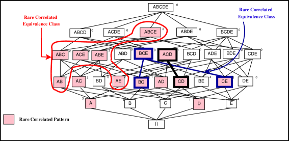
Figure 4.2: An example of rare correlated equivalence classes for minsupp = 4 and minbond = 0.2.

Example 18

Consider the extraction context sketched by Table 2.1 (Page 2.1). For minsupp = 4 and minbond = 0.2, we have $\mathcal{CRCP}$ = $\{$$A$, $D$, $AC$, $AD$, $ACD$, $BCE$, $ABCE$$\}$ and $\mathcal{MRCP}$ = $\{$$A$, $D$, $AB$, $AC$, $AD$, $AE$, $BC$, $CD$, $CE$$\}$.

An accurate representation of rare correlated patterns should determine, for an arbitrary pattern, whether it is rare correlated or not. If it is a rare correlated one, then this representation must allow drifting without information loss the values of its support and its bond measure. In this respect, the proposed representations in this work will be later shown to be perfect: their respective sizes never exceed that of the whole set of rare correlated patterns. In addition, since they are information lossless, these representations allow, whenever of need, the derivation of the whole set of rare correlated patterns efficiently.

To define our concise exact representations of rare correlated patterns, we are based on the notion of equivalence classes.

The first intuitive idea when defining a concise exact representation of the rare correlated patterns is to study whether the minimal elements or maximal ones of the equivalence classes would constitute an exact concise representation of the $\mathcal{RCP}$ set.

In this respect, it is important to remind that the $\mathcal{RCP}$ set results from the intersection of the order ideal of correlated patterns and the order filter of rare patterns. Thus, the $\mathcal{RCP}$ set does not induce neither an order ideal nor an order filter. In this situation, we take independently each set, to check whether the $\mathcal{CRCP}$ set or the $\mathcal{MRCP}$ set can provide a concise exact representation of the $\mathcal{RCP}$ set.

Let us analyze, in the following, each of the two sets separately:

- Let us begin with the $\mathcal{MRCP}$ set composed by the minimal elements of the rare correlated equivalence classes: In fact, due to the nature of its elements - minimal of their equivalence classes - this set allows for a given pattern $I$ to evaluate it towards the constraint of rarity. Indeed, it is enough to find an element $J$ $\in$ $\mathcal{MRCP}$ s.t. $J$ $\subseteq$ $I$ to decide whether $I$ is a rare pattern or not. If it is not the case, then $I$ is not a rare pattern. However, the set $\mathcal{MRCP}$ cannot determine, in the general case, whether $I$ is correlated or not (this is possible only if $I$ $\in$ $\mathcal{MRCP}$). Even if it exists $J$ $\in$ $\mathcal{MRCP}$ s.t. $J$ $\subset$ $I$, and even knowing that $J$ is correlated, we cannot confirm the correlation of nature of $I$ since this constraint is an anti-monotonic one (the fact that $J$ is correlated does not imply that $I$ is also correlated). Thus, the $\mathcal{MRCP}$ set, taken alone, cannot be an exact representation of the $\mathcal{RCP}$ set.

- Let us now treat the case of the $\mathcal{CRCP}$ of maximal elements of the rare correlated equivalence classes: Dually to the previous analysis of $\mathcal{MRCP}$, the $\mathcal{CRCP}$ set allows determining the nature of correlation for a given pattern $I$. If it is included in just one pattern $J$ $\in$ $\mathcal{CRCP}$, then $I$ is correlated. Otherwise, it is not a correlated one. However, due to their nature, the patterns composing the $\mathcal{CRCP}$ cannot in the general case derive the information about the status of rarity of a given pattern $I$ (this is possible only if $I$ $\in$ $\mathcal{CRCP}$). Even if it exists $J$ $\in$ $\mathcal{CRCP}$, s.t. $I$ $\subset$ $J$ and even if we already know that $J$ is rare, we cannot decide whether $I$ is rare or not since the constraint of rarity is monotone (the fact that $J$ is rare does not imply that $I$ is also rare). Thus, the $\mathcal{CRCP}$ set, taken alone, cannot be an exact representation of the $\mathcal{RCP}$ set. Nevertheless, it is proved from the previous analysis that the union of the $\mathcal{MRCP}$ set and the $\mathcal{CRCP}$ set would constitute an accurate concise representation of the $\mathcal{RCP}$ set of rare correlated patterns. The first alternative will be studied in the next sub-section, and will be then followed by two other optimizations in order to retain only the key elements for the lossless regeneration of the $\mathcal{RCP}$ set.

Based on this study, we introduce in the following subsections our new concise exact and approximate representations.

4.5.2 The $\mathcal{RCPR}$ concise exact representation

The first representation, that we introduce, is defined as follows:

Definition 39

The $\mathcal{RCPR}$ representation
Let $\mathcal{RCPR}$ be the concise exact representation of the $\mathcal{RCP}$ set based on the $\mathcal{CRCP}$ set and on the $\mathcal{MRCP}$ set of the minimal rare correlated patterns. The $\mathcal{RCPR}$ representation is equal to: $\mathcal{RCPR}$ = $\mathcal{CRCP}$ $\cup$ $\mathcal{MRCP}$. The support, Supp($\wedge I$), and the bond value, bond($I$) of each pattern $I$ of $\mathcal{RCPR}$ are exactly determined.

Example 19

Consider the extraction context sketched by Table 2.1 (Page 2.1). For minsupp = 4 and minbond = 0.2, while considering the $\mathcal{CRCP}$ set and $\mathcal{MRCP}$ set (cf. Example 18), the $\mathcal{RCPR}$ set is equal to: $\{$($A$, $3$, $\displaystyle\frac{3}{3}$), ($D$, $1$, $\displaystyle\frac{1}{1}$), ($AB$, $2$, $\displaystyle\frac{2}{5}$), ($AC$, $3$, $\displaystyle\frac{3}{4}$), ($AD$, $1$, $\displaystyle\frac{1}{3}$), ($AE$, $2$, $\displaystyle\frac{2}{5}$), ($BC$, $3$, $\displaystyle\frac{3}{5}$), ($CD$, $1$, $\displaystyle\frac{1}{4}$), ($CE$, $3$, $\displaystyle\frac{3}{5}$), ($ACD$, $1$, $\displaystyle\frac{1}{4}$), ($BCE$, $3$, $\displaystyle\frac{3}{5}$) and ($ABCE$, $2$, $\displaystyle\frac{2}{5}$)$\}$.

The following theorem proves that the $\mathcal{RCPR}$ representation is a lossless concise representation of the $\mathcal{RCP}$ set.

Theorem 1

The $\mathcal{RCPR}$ representation is a concise exact representation of the $\mathcal{RCP}$ set of rare correlated patterns.

Proof. Let $I$ $\subseteq$ $\mathcal{I}$. We distinct between three different cases:

a) If $I$ $\in$ $\mathcal{RCPR}$, then $I$ is a rare correlated pattern and we have its support and its bond values.

b) If $\nexists$ $J$ $\in$ $\mathcal{RCPR}$ as $J$ $\subseteq$ $I$ and $\nexists$ $Z$ $\in$ $\mathcal{RCPR}$ as $I$ $\subseteq$ $Z$, then $I$ $\notin$ $\mathcal{RCP}$ since $I$ does not belong to any rare correlated equivalence class.

c) If $I$ $\in$ $\mathcal{RCP}$. In fact, according to Proposition 6, $I$ is correlated since it is included in a correlated pattern, namely $Z$. It is also rare, since it contains a rare pattern, namely $J$. In this case, it is sufficient to localize the $f_{bond}$ closure of $I$ namely $F$. Then, the closed pattern $F$ belongs then to $\mathcal{RCPR}$ since $I$ is rare correlated and $\mathcal{RCPR}$ includes the $\mathcal{CRCP}$ set of closed rare correlated patterns. Therefore, $F$ = $min_{\subseteq}${$I_{1}$ $\in$ $\mathcal{RCPR}|$ $I$ $\subseteq$ $I_{1}$}. Since the $f_{bond}$ closure operator conserves the bond value and thus the conjunctive support (cf. Proposition 8), we have: bond($I$) = bond($F$) and Supp($\wedge I$) = Supp($\wedge F$).

Example 20

Consider the $\mathcal{RCPR}$ representation illustrated by the previous example. Let us consider each case separately. The pattern $AD$ $\in$ $\mathcal{RCPR}$. Thus, we have its support equal to 1 and its bond value equal to $\displaystyle\frac{1}{3}$. Even though, the pattern $BE$ is included in two patterns from the $\mathcal{RCPR}$ representation, namely $BCE$ and $ABCE$, $BE$ $\notin$ $\mathcal{RCP}$ since no element of $\mathcal{RCPR}$ is included in $BE$. Consider now the pattern $ABC$. It exists two patterns of $\mathcal{RCPR}$ proving that the pattern $ABC$ is a rare correlated one, namely $AB$ and $ABCE$, since $AB$ $\subseteq$ $ABC$ $\subseteq$ $ABCE$. The smallest pattern in $\mathcal{RCPR}$ covering $ABC$, i.e. its closure, is $ABCE$. Then, bond($ABC$) = bond($ABCE$) = $\displaystyle\frac{2}{5}$, and Supp($\wedge ABC$) = Supp($\wedge ABCE$) = 2.

We show through the following proposition that the $\mathcal{RCPR}$ representation is a perfect cover of the $\mathcal{RCP}$ set of rare correlated patterns.

Proposition 9

The $\mathcal{RCPR}$ representation is a perfect cover of the $\mathcal{RCP}$ set.

Proof. In fact, the size of the $\mathcal{RCPR}$ representation does never exceed that of the $\mathcal{RCP}$ set whatever the extraction context, the minsupp and the minbond values. Indeed, it is always true that ($\mathcal{CRCP}$ $\cup$ $\mathcal{MRCP}$) $\subseteq$ $\mathcal{RCP}$. Furthermore, knowing the conjunctive support of a given pattern and its bond value, we can compute the disjunctive support and thus the negative support. The interrogation of the representation $\mathcal{RCPR}$ can be based on the proof of Theorem 1. Thus, for a given pattern, thanks to the $\mathcal{RCPR}$ representation, we can determine whether it is rare correlated or not. If it is correlated rare, then its support as well as its bond value will be derived using the mechanism described by the previous theorem. The regeneration process of the whole set of rare correlated patterns can also be based on this theorem. This process starts by the smallest rare correlated patterns namely the minimal rare correlated patterns (constituting the $\mathcal{MRCP}$ set). These patterns belong to $\mathcal{RCPR}$ and we have therefore all their required information. It is then sufficient to localize for each minimal $M$ its closure $F$ which belongs to $\mathcal{RCPR}$ ($F$ $\in$ $\mathcal{CRCP}$ and this set is included in $\mathcal{RCPR}$). All the patterns which are included between $M$ and $F$ share the same support and bond value as $M$ and $F$ since they belong to the same rare correlated equivalence class.

Remark 3

It is important to mention that it is necessary to maintain for each pattern $I$ of the representation, at the same time Supp($\wedge I$) as well as bond($I$). On the one hand, bond($I$) is equal to the ratio between the conjunctive and the disjunctive support of $I$ and cannot determine the conjunctive support of $I$. On the other hand, knowing only the conjunctive support of $I$ is not sufficient to compute the bond value. The disjunctive support can be derived by the inclusion-exclusion identities only if we know all the conjunctive supports values of all the subsets of $I$ [Galambos and Simonelli, 2000]. Nevertheless, if $I$ is a rare correlated pattern, then its subsets are not necessarily rare correlated. Therefore, we don’t have the values of their conjunctive supports. Thus, we must keep track of the conjunctive support and the bond value for each element of the $\mathcal{RCPR}$ representation.

In this case, the closed and minimal patterns of the equivalence classes constitute, as shown previously, an interesting solution in order to represent with a concise and exact manner the $\mathcal{RCP}$ set. In fact, the localization of these patterns requires a limited neighborhood, i.e., just the strict supersets and subsets, and not all their subsets. In addition to this, the derivation of the support of the whole set of patterns from the closed and minimal non derivable can be done directly.

Remark 4

It is also interesting to mention that the fact to consider in the $\mathcal{RCPR}$ set, the union of the two sets $\mathcal{MRCP}$ and $\mathcal{CRCP}$ allows avoiding redundancy, because of the duplication of some patterns, which may appear in the representation when we consider the $\mathcal{MRCP}$ set and the $\mathcal{CRCP}$ set separately. For example, if we consider the example 19, we note that the elements ($A$, 3, $\displaystyle\frac{3}{3}$) , ($D$, 1, $\displaystyle\frac{1}{1}$), ($AC$, 3, $\displaystyle\frac{3}{4}$) and ($AD$, 1, $\displaystyle\frac{1}{3}$) belong to both sets $\mathcal{MRCP}$ and $\mathcal{CRCP}$. However, one advantage of saving each set separately allows the reduction of some tests of inclusion in the extraction of the representation. In fact, to make the choice between tolerating some duplication or benefiting from a potential reduction of the regeneration cost depends on the nature of the application where we can privilege either the optimization of the memory space or the derivation cost.

We propose in the following two refined versions of the $\mathcal{RCPR}$ representation, in order to further reduce the size of this representation.

4.5.3 The $\mathcal{MM}$$ax$$\mathcal{CR}$ concise exact representation

The first refinement is based on the fact that the $\mathcal{MRCP}$ set of minimal rare correlated patterns increased only by the maximal patterns according to the inclusion set, among the $\mathcal{CRCP}$ set of closed rare correlated patterns is sufficient to faithfully represent the $\mathcal{RCP}$ set. In this respect, we define the $\mathcal{M}$$ax$$\mathcal{CRCP}$ set of maximal closed rare correlated patterns as follows:

Definition 40

The $\mathcal{M}$$ax$$\mathcal{CRCP}$ set of maximal closed rare correlated patterns
The $\mathcal{M}$$ax$$\mathcal{CRCP}$ set is composed by the patterns which are closed correlated rare ones (cf. Definition 37, page 37) and at the same time they are maximal correlated (cf. Definition 30, page 30). Then, we have $\mathcal{M}$$ax$$\mathcal{CRCP}$ = $\mathcal{CRCP}$ $\cap$ $\mathcal{M}ax$$\mathcal{CP}$.

The $\mathcal{M}$$ax$$\mathcal{CRCP}$ set is then limited to the elements of the $\mathcal{M}ax$$\mathcal{CP}$ set which are also rare, in addition of being the largest correlated patterns.

Example 21

Consider the extraction context sketched by Table 2.1(Page 2.1). For minsupp = 4 and minbond = 0.2, we have $\mathcal{M}$$ax$$\mathcal{CRCP}$ = $\{$$ACD$, $ABCE$$\}$.

We define in the following the representation based on the $\mathcal{M}$$ax$$\mathcal{CCRP}$ set.

Definition 41

The $\mathcal{MM}$$ax$$\mathcal{CR}$ representation
Let $\mathcal{MM}$$ax$$\mathcal{CR}$ be the representation based on the $\mathcal{MRCP}$ set and the $\mathcal{M}$$ax$$\mathcal{CRCP}$. We have, $\mathcal{MM}$$ax$$\mathcal{CR}$ = $\mathcal{MRCP}$ $\cup$ $\mathcal{M}$$ax$$\mathcal{CRCP}$. For each element $I$ of the $\mathcal{MM}ax\mathcal{CR}$, the support, Supp($\wedge I$), and the bond value, bond($I$) are computed.

Example 22

Consider the extraction context sketched by Table 2.1 (Page 2.1). For minsupp = 4 and minbond = 0.2, the representation $\mathcal{MM}ax\mathcal{CR}$ is equal to: $\{$($A$, $3$, $\displaystyle\frac{3}{3}$), ($D$, $1$, $\displaystyle\frac{1}{1}$), ($AB$, $2$, $\displaystyle\frac{2}{5}$), ($AC$, $3$, $\displaystyle\frac{3}{4}$), ($AD$, $1$, $\displaystyle\frac{1}{3}$), ($AE$, $2$, $\displaystyle\frac{2}{5}$), ($BC$, $3$, $\displaystyle\frac{3}{5}$), ($CD$, $1$, $\displaystyle\frac{1}{4}$), ($CE$, $3$, $\displaystyle\frac{3}{5}$), ($ACD$, $1$, $\displaystyle\frac{1}{4}$), and ($ABCE$, $2$, $\displaystyle\frac{2}{5}$)$\}$. We remark that, for this example, the unique element of the $\mathcal{RCPR}$ representation that does not belong to the $\mathcal{MM}$$ax$$\mathcal{CR}$ representation is, the pattern $BCE$. In fact, the closed patterns that were removed, i.e., $A$, $D$, $AC$ and $AD$, are also minimal. Indeed, the $\mathcal{MM}$$ax$$\mathcal{CR}$ representation would be more optimized than do the $\mathcal{RCPR}$ representation, if the sets $\mathcal{MRCP}$ and $\mathcal{CRCP}$ were saved separately (cf. Remark 4). In fact, the duplicate storage of the patterns $A$, $D$, $AC$ and $AD$ is avoided.

Theorem 2 proves that the $\mathcal{MM}$ax$\mathcal{CR}$ set is a lossless representation of the $\mathcal{RCP}$ set.

Theorem 2

The $\mathcal{MM}$ax$\mathcal{CR}$ set is an exact concise representation of the $\mathcal{RCP}$ set of rare correlated patterns.

Proof. Let a pattern $I$ $\subseteq$ $\mathcal{I}$. We distinguish between three cases:

a) If $I$ $\in$ $\mathcal{MM}$$ax$$\mathcal{CR}$, then $I$ is a rare correlated pattern and we have its support and bond values.

b) If $\nexists$ $J$ $\in$ $\mathcal{MM}$$ax$$\mathcal{CR}$ as $J$ $\subseteq$ $I$ or $\nexists$ $Z$ $\in$ $\mathcal{MM}$$ax$$\mathcal{CR}$ as $I$ $\subseteq$ $Z$, then $I$ $\notin$ $\mathcal{RCP}$ since $I$ do not belong to any rare correlated equivalence class.

c) Else, $I$ $\in$ $\mathcal{RCP}$. In fact, according to Proposition 6, $I$ is a correlated pattern since it is included in a correlated pattern, say $Z$. It is also rare since it contains a rare pattern, say $J$. Since $I$ is a rare correlated pattern and the representation $\mathcal{MM}$$ax$$\mathcal{CR}$ includes the $\mathcal{MRCP}$ set containing the minimal elements of the different rare correlated equivalence classes, this representation has at least one element of the equivalence class of $I$, particularly all the minimal patterns of its class.
Since both the conjunctive support and the bond measure decrease as far the size of the patterns is lowered, the support and bond values of $I$ are equal to the minimal values of the measures associated to its subsets belonging to the $\mathcal{MM}$$ax$$\mathcal{CR}$ representation. We deduce then that:
$\bullet$ Supp($\wedge$$I$) = $min$$\{$Supp($\wedge$$I_{1}$)$|$ $I_{1}$ $\in$ $\mathcal{MM}$$ax$$\mathcal{CR}$ and $I_{1}$ $\subseteq$ $I$$\}$; and
$\bullet$ bond($I$) = $min$$\{$bond($I_{1}$)$|$ $I_{1}$ $\in$ $\mathcal{MM}$$ax$$\mathcal{CR}$ and $I_{1}$ $\subseteq$ $I$$\}$.

Example 23

Consider the $\mathcal{MM}$$ax$$\mathcal{CR}$ presented in Example 22. The treatment of the first and second cases is similar to the first two cases of the $\mathcal{RCPR}$ representation (cf. Example 20). The case of the pattern $ABE$ is illustrative of the third alternative. In fact, it exists two patterns, from the $\mathcal{MM}$$ax$$\mathcal{CR}$ representation, which makes $ABE$ a rare correlated pattern, namely $AB$ and $ABCE$ ($AB$ $\subseteq$ $ABE$ $\subseteq$ $ABCE$). The elements of the $\mathcal{MM}$$ax$$\mathcal{CR}$ representation which are included in $ABE$ are $AB$ and $AE$. Consequently, Supp($\wedge$$ABE$) = $min$$\{$Supp($\wedge$$AB$), Supp($\wedge$$AE$)$\}$ = $min$$\{$2, 2$\}$ = 2, and bond($ABE$) = $min$$\{$bond($AB$), bond($AE$)$\}$ = $min$$\{$$\displaystyle\frac{2}{5}$, $\displaystyle\frac{2}{5}$$\}$ = $\displaystyle\frac{2}{5}$.

Since the $\mathcal{MM}$$ax$$\mathcal{CR}$ representation is included in the $\mathcal{RCPR}$ representation, and the latter is a perfect cover of the $\mathcal{RCP}$ set, then we deduce that the $\mathcal{MM}$$ax$$\mathcal{CR}$ representation is also a perfect cover of the $\mathcal{RCP}$ set. In the next sub-section, we present another refinement of the $\mathcal{RCPR}$ representation.

4.5.4 The $\mathcal{M}$$in$$\mathcal{MCR}$ concise exact representation

Dually to the previous definition, it is sufficient to maintain in the $\mathcal{RCPR}$ representation, just the minimal elements, according to the inclusion set, among the $\mathcal{MRCP}$ set. The pruning of the other elements from the $\mathcal{MRCP}$ set will be shown to be information lossless during the regeneration of the whole set of rare correlated patterns. The $\mathcal{M}$$in$$\mathcal{MRCP}$ set of minimal elements among the $\mathcal{MRCP}$, is thus defined as follows:

Definition 42

The $\mathcal{M}$$in$$\mathcal{MRCP}$ set of the minimal elements of the $\mathcal{MRCP}$ set
The $\mathcal{M}$$in$$\mathcal{MRCP}$ set is composed by the patterns which are minimal rare correlated patterns (cf. Definition 38, page 38) and at the same time minimal rare patterns (cf. Definition 5, page 5). Thus, $\mathcal{M}in\mathcal{MRCP}$ = $\mathcal{MRCP}$ $\cap$ $\mathcal{M}in\mathcal{RP}$.

The $\mathcal{M}in\mathcal{MRCP}$ set is then limited by the minimal rare correlated patterns which are also minimal rare (In addition to being the smallest rare patterns).

Example 24

Consider the extraction context sketched by Table 2.1 (Page 2.1). For minsupp = 4 and minbond = 0.2, we have $\mathcal{M}in$$\mathcal{MRCP}$ = $\{$$A$, $D$, $BC$, $CE\}$.

The following definition introduces the representation based on the $\mathcal{M}in\mathcal{MCRP}$ set.

Definition 43

The $\mathcal{M}in\mathcal{MCR}$ representation
Let $\mathcal{M}in\mathcal{MCR}$ be the representation based on the $\mathcal{M}in\mathcal{MCRP}$ set and the $\mathcal{CRCP}$ set. We have $\mathcal{M}in\mathcal{MCR}$ = $\mathcal{CRCP}$ $\cup$ $\mathcal{M}in\mathcal{MRCP}$. For each element $I$ of $\mathcal{M}in\mathcal{MCR}$, its support Supp($\wedge I$) and its bond value bond($I$) are computed.

Example 25

Consider the extraction context sketched by Table 2.1 (Page 2.1). For minsupp = 4 and minbond = 0.2, we have the $\mathcal{M}$$in$$\mathcal{MCR}$ = $\{$($A$, 3, $\displaystyle\frac{3}{3}$), ($D$, 1, $\displaystyle\frac{1}{1}$), ($AC$, 3, $\displaystyle\frac{3}{4}$), ($AD$, 1, $\displaystyle\frac{1}{3}$), ($BC$, 3, $\displaystyle\frac{3}{5}$), ($CE$, 3, $\displaystyle\frac{3}{5}$), ($ACD$, 1, $\displaystyle\frac{1}{4}$), ($BCE$, 3, $\displaystyle\frac{3}{5}$), and ($ABCE$, 2, $\displaystyle\frac{2}{5}$)$\}$. We remark that, this representation has three elements less than the $\mathcal{RCPR}$ representation, namely $AB$, $AE$ and $CD$.

The following theorem proves that this representation is also a lossless reduction of the $\mathcal{RCP}$ set.

Theorem 3

The $\mathcal{M}$$in$$\mathcal{MCR}$ representation is a concise exact representation of the $\mathcal{RCP}$ set of rare correlated patterns.

Proof. Let $I$ $\subseteq$ $\mathcal{I}$. We distinguish between three different cases:

a) If $I$ $\in$ $\mathcal{M}$$in$$\mathcal{MCR}$, then $I$ is a rare correlated pattern and we know its support as well as its bond value.

b) If $\nexists$ $J$ $\in$ $\mathcal{M}$$in$$\mathcal{MCR}$ as $J$ $\subseteq$ $I$ or $\nexists$ $Z$ $\in$ $\mathcal{M}$$in$$\mathcal{MCR}$ as $I$ $\subseteq$ $Z$, then $I$ $\notin$ $\mathcal{RCP}$ since $I$ does not belong to any rare correlated equivalence class.

c) Otherwise, $I$ $\in$ $\mathcal{RCP}$. In fact, according to Proposition 6, $I$ is correlated since it is included in a correlated pattern, namely $Z$. It is also rare since it includes a rare pattern, namely $J$. Since the $\mathcal{CRCP}$ set belongs to $\mathcal{M}$$in$$\mathcal{MCR}$, it is enough to localize the closed pattern associated to $I$, namely $F$, equal to: $F$ = $min_{\subseteq}${$I_{1}$ $\in$ $\mathcal{M}$$in$$\mathcal{MCR}$ $|$ $I$ $\subseteq$ $I_{1}$}. Then, bond($I$) = bond($F$) and Supp($\wedge I$) = Supp($\wedge F$).


The treatment of these three cases is similar to those of the $\mathcal{RCPR}$ representation, (cf. Example 20 page 20). The $\mathcal{M}$$in$$\mathcal{MCR}$ representation also constitutes a perfect cover of the $\mathcal{RCP}$ set, since it is included in the $\mathcal{RCPR}$ representation.

After the introduction of our exact condensed representations, we deal in the following with the approximate concise representation.

4.5.5 The $\mathcal{M}$$in$$\mathcal{MM}$$ax$$\mathcal{CR}$ concise approximate representation

The approximate concise representation, that we introduce, is defined as follows:

Definition 44

The $\mathcal{M}$$in$$\mathcal{MM}$$ax$$\mathcal{CR}$ representation
Let $\mathcal{M}$$in$$\mathcal{MM}$$ax$$\mathcal{CR}$ be the representation based on the $\mathcal{M}ax$$\mathcal{CRCP}$ set and the $\mathcal{M}in$$\mathcal{MRCP}$ set. We have $\mathcal{M}$$in$$\mathcal{MM}$$ax$$\mathcal{CR}$ = $\mathcal{M}ax$$\mathcal{CRCP}$ $\cup$ $\mathcal{M}in$$\mathcal{MRCP}$. For each element $I$ of $\mathcal{M}$$in$$\mathcal{MM}$$ax$$\mathcal{CR}$, the support Supp($\wedge$$I$) and the bond value bond($I$) are computed.

Example 26

We have, $\mathcal{M}in$$\mathcal{MRCP}$ = $\{$$A$, $D$, $BC$, $CE$$\}$ (cf. Example 24) and $\mathcal{M}ax$$\mathcal{CRCP}$ = $\{$$ACD$, $ABCE$$\}$ (cf. Example 21). Therefore, $\mathcal{M}$$in$$\mathcal{MM}$$ax$$\mathcal{CR}$ = $\{$($A$, 3, $\displaystyle\frac{3}{3}$), ($D$, 1, $\displaystyle\frac{1}{1}$), ($BC$, 3, $\displaystyle\frac{3}{5}$), ($CE$, 3, $\displaystyle\frac{3}{5}$), ($ACD$, 1, $\displaystyle\frac{1}{4}$), ($ABCE$, 2, $\displaystyle\frac{2}{5}$)$\}$.

In the previous example, the $\mathcal{M}$$in$$\mathcal{MM}$$ax$$\mathcal{CR}$ representation has six elements less than the $\mathcal{RCPR}$ set, eleven elements less than the $\mathcal{MM}$$ax$$\mathcal{CR}$ set and one element less than $\mathcal{M}$$in$$\mathcal{MCR}$. However, this representation can not exactly derive the support and the bond values of a given rare correlated pattern.

Theorem 4

The $\mathcal{M}$$in$$\mathcal{MM}$$ax$$\mathcal{CR}$ is an approximate concise representation of the $\mathcal{RCP}$ set of the rare correlated patterns.

Proof. For a given pattern $I$ $\subseteq$ $\mathcal{I}$, we can determine thanks to this representation whether $I$ is rare correlated or not. It suffices to find two patterns $J$ and $Z$ belonging to $\mathcal{M}$$in$$\mathcal{MM}$$ax$$\mathcal{CR}$ such as $J$ $\subseteq$ $I$ $\subseteq$ $Z$. If $J$ or $Z$ can not be found, then $I$ $\notin$ $\mathcal{RCP}$. However, the support and bond values can be exactly derived only if $I$ $\in$ $\mathcal{M}$$in$$\mathcal{MM}$$ax$$\mathcal{CR}$. Otherwise, this representation can not offer an exact derivation of these values, since it may not contain any representative element of the equivalence class of $I$ (i.e. neither the closed pattern if it does not belong to the $\mathcal{M}ax$$\mathcal{CRCP}$ set nor to the associated minimal if they don’t belong to the $\mathcal{M}in$$\mathcal{MRCP}$ set). We propose in this case an approximate process in order to get these values. We define, in this regard, the maximal and minimal borders of the conjunctive, the disjunctive and the bond value of a correlated rare pattern $I$. Let,

$\bullet$ R1 = $\max$$\{$Supp($\wedge$$F$), $F$ $\in$ $\mathcal{M}ax$$\mathcal{CRCP}$ $|$ $I$ $\subseteq$ $F$$\}$,

$\bullet$ R2 = $\min$$\{$Supp($\wedge$$G$), $G$ $\in$ $\mathcal{M}in$$\mathcal{MRCP}$ $|$ $G$ $\subseteq$ $I$$\}$,

$\bullet$ R3 = $\min$$\{$Supp($\vee$$F$), $F$ $\in$ $\mathcal{M}ax$$\mathcal{CRCP}$ $|$ $I$ $\subseteq$ $F$$\}$ and

$\bullet$ R4 = $\max$$\{$Supp($\vee$$G$), $G$ $\in$ $\mathcal{M}in$$\mathcal{MRCP}$ $|$ $G$ $\subseteq$ $I$$\}$.

We define, therefore, the minimal and maximal borders in terms of R1 and of R2 as follows. Let MinConj be the minimal border of the conjunctive support of the pattern $I$, i.e., MinConj = $\min$(R1, R2). Let MaxConj be the maximal border of the conjunctive support of the pattern $I$, i.e., MaxConj = $\max$(R1, R2).

According to the disjunctive support of a given pattern $I$, we define the maximal and minimal borders in terms of R3 and of R4 as follows. Let MinDisj be the minimal border of the disjunctive support, MinDisj = $\min$(R3, R4) and let MaxDisj be the maximal border of the disjunctive support, MaxDisj = $\max$(R3, R4).

Consequently, the conjunctive support of a rare correlated pattern $I$ will be included between MinConj and MaxConj. In the same way, the disjunctive support will be included between MinDisj and MaxDisj. Formally, we have Supp($\wedge$$I$) $\in$ $[$MinConj, MaxConj$]$ and Supp($\vee$$I$) $\in$ $[$MinDisj, MaxDisj$]$.

Therefore, we define the minimal and maximal borders of the bond value of a rare correlated pattern $I$ in terms of MinConj, MinDisj, MaxConj and MaxDisj as follows.

Since MinDisj $\leq$ Supp($\vee$$I$) $\leq$ MaxDisj, then we have $\displaystyle\frac{1}{\textit{MaxDisj}}$ $\leq$ $\displaystyle\frac{1}{\textit{Supp}\textsc{(}\vee I\textsc{)}}$ $\leq$ $\displaystyle\frac{1}{\textit{MinDisj}}$.

As Supp($\wedge$I) $>$ 0 then we can deduce that, $\displaystyle\frac{\textit{Supp}\textsc{(}\wedge I\textsc{)}}{\textit{MaxDisj}}$ $\leq$ $\displaystyle\frac{\textit{Supp}\textsc{(}\wedge I\textsc{)}}{\textit{Supp}\textsc{(}\vee I\textsc{)}}$ $\leq$ $\displaystyle\frac{\textit{Supp}\textsc{(}\wedge I\textsc{)}}{\textit{MinDisj}}$. This is equivalent to, $\displaystyle\frac{\textit{Supp}\textsc{(}\wedge I\textsc{)}}{\textit{MaxDisj}}$ $\leq$ bond($I$) $\leq$ $\displaystyle\frac{\textit{Supp}\textsc{(}\wedge I\textsc{)}}{\textit{MinDisj}}$. Already, MinConj $\leq$ Supp($\wedge$ $I$) , then $\displaystyle\frac{\textit{MinConj}}{\textit{MaxDisj}}$ $\leq$ bond($I$). Besides, Supp($\wedge$$I$) $\leq$ MaxConj then bond($I$) $\leq$ $\displaystyle\frac{\textit{MaxConj}}{\textit{MinDisj}}$. We then have, $\displaystyle\frac{\textit{MinConj}}{\textit{MaxDisj}}$ $\leq$ bond($I$) $\leq$ $\displaystyle\frac{\textit{MaxConj}}{\textit{MinDisj}}$.

We conclude then that, bond($I$) $\in$ $[$Minbond, Maxbond$]$, with Minbond = $\displaystyle\frac{\textit{MinConj}}{\textit{MaxDisj}}$ and Maxbond = $\displaystyle\frac{\textit{MaxConj}}{\textit{MinDisj}}$.

Example 27

With respect to Example 26, we have $ABE$ is a correlated rare pattern since ($A$ $\subset$ $ABE$ $\subset$ $ABCE$). The conjunctive, disjunctive and the bond value of $ABE$ are approximated as follows:
$\bullet$ R1 = Supp($\wedge$$ABCE$) = 2,
$\bullet$ R2 = Supp($\wedge$$A$) = 3,
$\bullet$ R3 = Supp($\vee$$ABCE$) = 5,
$\bullet$ R4 = Supp($\vee$$A$) = 5.
Thus, we have MinConj = $\min$(R1, R2) = $\min$(2, 3) = 2, MaxConj = $\max$(R1, R2) = $\max$(2, 3) = 3, and $\min$(R3, R4) = $\max$(R3, R4) = $\min$(5, 5) = $\max$(5, 5) = 5. We have, therefore, MinDisj = MaxDisj = 5. This implies that, Minbond = $\displaystyle\frac{\textit{MinConj}}{\textit{MaxDisj}}$ = $\displaystyle\frac{2}{5}$ and Maxbond = $\displaystyle\frac{\textit{MaxConj}}{\textit{MinDisj}}$ = $\displaystyle\frac{3}{5}$.

Consequently, we have Supp($\wedge$$ABE$) $\in$ $[$2, 3$]$, Supp($\vee$$ABE$) $\in$ $[$5, 5$]$ so Supp($\vee$$ABE$) = 5 and bond($ABE$) $\in$ $[$$\displaystyle\frac{2}{5}$, $\displaystyle\frac{3}{5}$$]$.

We remark, according to the extraction context illustrated by Table 2.1 (Page 2.1 ), that the conjunctive, disjunctive and the bond values of the pattern $ABE$ corresponds respectively to 2, 5 and $\displaystyle\frac{2}{5}$. These values does not contradict the previously obtained approximate values. We affirm that the approximation mechanism offered by the approximate concise representation $\mathcal{RM}$$in$$\mathcal{MM}$$ax$$\mathcal{F}$ is valid.

After presenting the condensed representations associated to the rare correlated patterns, we focus on the next section on the condensed representation associated to the $\mathcal{FCP}$ set of frequent correlated patterns

4.6 Condensed representation of frequent correlated patterns

Based on the $f_{bond}$ closure operator, a condensed representation which cover the frequent correlated patterns was proposed in [Ben Younes et al., 2010]. This representation is based on the frequent closed correlated patterns. The proposed representation is considered more concise than the representation based on minimal correlated patterns thanks to the fact that a $f_{bond}$ equivalence class always contains only one closed pattern, but potentially several minimal patterns.

Before introducing the representation, let us define the two discussed sets of frequent closed correlated patterns and of the frequent minimal correlated pattern associated to the $f_{bond}$ operator.

Definition 45

Frequent closed correlated pattern
The set $\mathcal{FCCP}$ of frequent closed correlated patterns is equal to: $\mathcal{FCCP}$ = $\{$ $I$ $\in$ $\mathcal{CCP}$ $|$ Supp($I$) $\geq$ minsupp$\}$.

Definition 46

Frequent minimal correlated pattern
Let I $\in$ $\mathcal{FCP}$. The pattern I is said to be minimal if and only if $\forall$ $i$ $\in$ I, bond(I) $<$ bond(I$\backslash$$\{i\}$) or, equivalently, $\nexists$ $I_{1}$ $\subset$ $I$ such that $f_{bond}\textsc{(}I\textsc{)}$ = $f_{bond}\textsc{(}I_{1}\textsc{)}$.

Example 28

Consider the extraction context sketched by Table 2.1 (Page 2.1 ). For minsupp = 4 and minbond = 0.20, the $\mathcal{FCCP}$ set of frequent closed correlated pattern is equal to: $\{$( (C, 4, 4), (BE, 4, 4)$\}$ while the frequent minimal correlated pattern are the items (B, 4, 4), (C, 4, 4) and (E, 4, 4).

Now, let us define the new concise representation of frequent correlated patterns based on the frequent closed correlated patterns associated to the bond measure.

Definition 47

The representation $\mathcal{RFCCP}$ based on the set of frequent closed correlated patterns associated to $f_{bond}$ is defined as follows:

$\mathcal{RFCCP}=\{$(I, Supp($\wedge$I), Supp($\vee$I)) $|$ $I\in\mathcal{FCCP}$ $\}$.

Example 29

Consider the extraction context sketched by Table 2.1 (Page 2.1 ). For minsupp = 4 and minbond = 0.20, the representation $\mathcal{RFCCP}$ of the $\mathcal{FCP}$ set is equal to: $\{$( (C, 4, 4), (BE, 4, 4)$\}$.

The next theorem proves that the proposed $\mathcal{RFCCP}$ representation is a condensed exact representation of the $\mathcal{FCP}$ set of frequent correlated patterns.

Theorem 5

The representation $\mathcal{RFCCP}$ constitutes an exact concise representation of the $\mathcal{FCP}$ set.

Proof. Thanks to a reasoning by recurrence, we will demonstrate that, for an arbitrary pattern $I\subseteq\mathcal{I}$, its $f_{bond}$ closure, $f_{bond}$($I$), belongs to $\mathcal{FCCP}$ if it is frequent correlated. In this regard, let $\mathcal{FMCP}_{k}$ be the set of frequent minimal correlated patterns of size $k$ and $\mathcal{FCCP}_{k}$ be the associated set of closures by $f_{bond}$. The hypothesis is verified for single items $i$ inserted in $\mathcal{FMCP}_{1}$, and their closures $f_{bond}\textsc{(}i\textsc{)}$ are inserted in $\mathcal{FCCP}_{1}$ if $\textit{Supp}\textsc{(}\wedge i\textsc{)}\geq$ minsupp (since $\forall$ $i$ $\in$ $\mathcal{I}$, $\textit{bond}\textsc{(}i\textsc{)}$ $=$ $1$ $\geq$ minbond). Thus, $f_{bond}\textsc{(}i\textsc{)}\in\mathcal{FCCP}$. Now, suppose that $\forall I\subseteq\mathcal{I}$ such as $|I|=n$. We have $f_{bond}\textsc{(}I\textsc{)}\in\mathcal{FCCP}$ if $I$ is frequent correlated. We show that, $\forall I\subseteq\mathcal{I}$ such as $|I|$ $=$ ($n+1$), we have $f_{bond}\textsc{(}I\textsc{)}\in\mathcal{FCCP}$ if $I$ is frequent correlated. Let $I$ be a pattern of size ($n+1$). Three situations are possible:
(a) if $I\in\mathcal{FCCP}$, then necessarily $f_{bond}\textsc{(}I\textsc{)}\in\mathcal{FCCP}$ since $f_{bond}$ is idempotent.
(b) if $I$ $\in\mathcal{FMCP}_{n+1}$, then $f_{bond}\textsc{(}I\textsc{)}\in\mathcal{FCCP}_{n+1}$ and, hence, $f_{bond}\textsc{(}I\textsc{)}\in\mathcal{FCCP}$.
(c) if $I$ is neither closed nor minimal – $I\notin\mathcal{FCCP}$ and $I\notin\mathcal{FMCP}_{n+1}$ – then $\exists I_{1}\subset I$ such as $|I_{1}|$ $=$ $n$ and bond($I$) $=$ bond($I_{1}$). In fact, $f_{bond}$($I$) $=$ $f_{bond}$($I_{1}$), and $I$ is then frequent correlated. Moreover, using the hypothesis, we have $f_{bond}$($I_{1}$) $\in$ $\mathcal{FCCP}$ and, hence, $f_{bond}$($I$) $\in$ $\mathcal{FCCP}$.

4.7 Conclusion

In this chapter, we studied the frequent correlated and the rare correlated patterns according to the bond correlation measure. We equally described the equivalence classes induced by the $f_{bond}$ closure operator associated to the bond measure. Then, we introduced the condensed exact and approximate representations associated to rare correlated patterns and also to frequent correlated ones. We proved their theoretical properties of accuracy and compactness. This chapter was concluded with the condensed representation associated to the $\mathcal{FCP}$ set of frequent correlated patterns. In the next chapter, we propose a mining approach, called GMJP, allowing the extraction of both frequent correlated patterns, rare correlated patterns and their associated concise representations.

Chapter 5 Extraction Approach of Correlated Patterns and associated Condensed Representations

5.1 Introduction

This chapter is dedicated to the presentation of our approach called Gmjp. Section 5.2 is devoted to the analysis of the different integration mechanism of the constraints of frequency and of correlation. Section 5.3 presents the description of the Gmjp approach, going from general to specificities. We describe the three different steps of Gmjp, then we present Opt-Gmjp the optimized version of the Gmjp algorithm in Section 5.4. We compute the theoretical approximate time complexity of Gmjp in Section 5.5. In Section 5.6, we describe the regeneration strategy of the rare correlated patterns from the $\mathcal{RCPR}$ representation. We conclude the chapter in Section 5.7.

5.2 Integration mechanism of the constraints

This chapter is dedicated to the presentation of the extraction approach of both frequent correlated and rare correlated itemsets as well as their associated condensed representations. For the case of the frequent correlated patterns, the extraction process is straightforward since the set of frequent correlated patterns induces an ideal order on the itemset lattice and fulfills an anti-monotonic constraint. Whereas, for the rare correlated patterns, we have to handle two constraints of distinct types: monotonic and anti-monotonic. The evaluation order of the constraints is of paramount importance given the opposite nature of the handled constraints of rarity and of correlation. Thus, we distinguish two different possible scenarios:

$\bullet$ First Scenario: We first apply the rarity constraint and the associated conjunctive closure operator, then we apply the correlation constraint.

$\bullet$ Second Scenario: We apply the correlation constraint and the associated $f_{bond}$ closure operator, then we integrate the rarity constraint.

These two scenarios will be analyzed in what follows in order to justify our choice of the adequate scenario in our proposed extraction approach.

5.2.1 First Scenario

In this case, we firstly extract the rare patterns. Then, we filter the retained rare patterns by the correlation constraint. Thus, only the rare correlated patterns are retained. In this situation, in order to reduce the redundancy among the rare correlated itemsets, we apply the conjunctive closure operator associated to the conjunctive support [Ganter and Wille, 1999]. This latter splits the itemset lattice into disjoint equivalence classes where, for each pattern, this closure preserve only the conjunctive support. Consequently, the whole set of the itemsets that appear in the same transactions are merged into the same equivalence class. They share the same conjunctive support, the same conjunctive closure, but they have eventually different disjunctive supports. Thereby, these rare equivalence classes, i.e, those containing just rare patterns, are evaluated by the anti-monotonic constraint of correlation. The rare patterns belonging to the same class, are then divided into rare correlated patterns and rare non-correlated ones as shown by Figure 5.1.

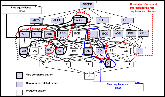
Figure 5.1: Effect of the integration of the correlation constraint for minsupp = 3 and minbond = 0.3.

Example 30

Let us consider the extraction context given by Table 2.1 (Page 2.1). For minsupp = 3, we distinguish two rare equivalence classes $\mathcal{C}_{1}$ and $\mathcal{C}_{2}$ shown in Figure 5.1 and composed by the following elements :

• $\mathcal{C}_{1}$ contains the itemsets D, AD, CD and ACD. $\mathcal{C}_{1}$ has the value of conjunctive support equal to 1 and the conjunctive closed pattern is ACD.

• $\mathcal{C}_{2}$ contains the itemsets AB, AE, ABC, ABE, ACE, and ABCE. $\mathcal{C}_{2}$ has the value of conjunctive support equal to 2 and the conjunctive closed pattern is ABCE.

Let us apply the correlation constraint for a minimal threshold minbond = 0.3. For the $\mathcal{C}_{1}$ equivalence class, the patterns $\{$(D, 1, $\displaystyle\frac{1}{1}$), (AD, 1, $\displaystyle\frac{1}{3}$)$\}$ are rare correlated whereas (CD, 1, $\displaystyle\frac{1}{4}$), (ACD, 1, $\displaystyle\frac{1}{4}$) are rare non-correlated itemsets. This is explained by the fact that the elements of the equivalence class $\mathcal{C}_{1}$ do not share the same disjunctive support, consequently they do not share the same bond value. On the other side, all of the elements of the equivalence class $\mathcal{C}_{2}$ are rare correlated.

5.2.2 Second Scenario

The second scenario consists in extracting all of the correlated patterns and partitioning them into equivalence classes thanks to the $f_{bond}$ closure operator, then filtering out the obtained equivalence classes by the rarity constraint. In fact, all the itemsets belonging to the same equivalence class share obviously the same conjunctive, disjunctive supports and the same bond measure. Consequently, when considering the anti-monotonic constraint of correlation, we can distinguish two kinds of classes namely: correlated classes and non-correlated ones. The good question that we have to think about it is what will be the effect of applying the monotonic constraint of rarity within this classes? In other words, how these equivalence classes will be affected by the interception of the rarity constraint?

In fact, the $f_{bond}$ closure operator preserves the bond value, the conjunctive, the disjunctive as well as the negative supports in the same equivalence class. Consequently, all the itemsets belonging to the same equivalence class present the same behavior regarding to the constraints of rarity and those of correlation. In this respect, the correlated patterns of an equivalence class, are either rare correlated or they are frequent correlated. This property also hold for the non correlated equivalence classes. Therefore, these classes are not affected by the application of the rarity constraint. As shown by Figure 5.2, we have correlated frequent classes, correlated rare classes, non correlated frequent classes and non correlated rare classes.

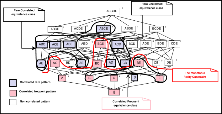
Figure 5.2: Effect of the application of the rarity constraint for minsupp = 3 and minbond = 0.2.

5.2.3 Summary

The equivalence classes induced by the $f_{bond}$ closure operator present pertinent characteristics. In fact, this privilege is not offered by the conjunctive closure operator [Ganter and Wille, 1999]. In fact, the state of a given pattern in an equivalence class induced by the conjunctive closure operator is not representative of the state of the other patterns of its same class. In this regard, we are motivated for the application of the second scenario within the design of our mining approach.

We introduce, in the next section, our new Gmjp approach ${}^{\textsc{(}}$${}^{\textsc{)}}$.

5.3 The Gmjp approach

We introduce in this section the Gmjp approach which allows, according to the user’s input parameters, the extraction of the desired output. As shown by Figure 5.3, four different scenarios are possible for running the Gmjp approach:
$\bullet$ First Scenario: outputs the whole set $\mathcal{FCP}$ of frequent correlated patterns,
$\bullet$ Second Scenario: outputs the $\mathcal{RFCCP}$ concise exact representation of the $\mathcal{FCP}$ set,
$\bullet$ Third Scenario: outputs the whole set $\mathcal{RCP}$ of rare correlated patterns,
$\bullet$ Fourth Scenario: outputs the $\mathcal{RCPR}$ concise exact representation of the $\mathcal{RCP}$ set.

The Gmjp algorithm takes as an input a dataset $\mathcal{D}$, a minimal support threshold minsupp and a minimal correlation threshold minbond. We mention that Gmjp determines exactly the support and the bond values of each pattern of the desired output according to the user’s parameters.

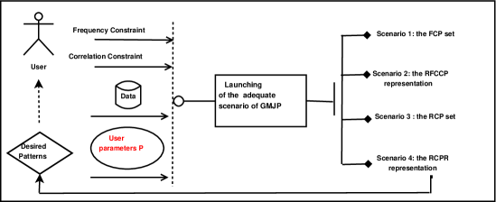
Figure 5.3: Overview of Gmjp approach.

5.3.1 Overview of the approach

We illustrate the different steps of Gmjp when running the fourth script aiming to extract the $\mathcal{RCPR}$ representation. Our choice of this fourth scenario is motivated by the fact that the extraction of the $\mathcal{RCPR}$ representation corresponds to the most challenging mining task for Gmjp.

In fact, $\mathcal{RCPR}$ is composed by the set of rare correlated patterns which results from the intersection of two theories [Mannila and Toivonen, 1997] induced by the constraints of correlation and rarity. So, this set is neither an order ideal nor an order filter. Therefore, the localization of the elements of the $\mathcal{RCPR}$ representation is more difficult than the localization of theories corresponding to the conjunction of constraints of the same nature. Indeed, the conjunction of anti-monotonic constraints (resp. monotonic) is an anti-monotonic constraint (resp. monotonic) [Bonchi and Lucchese, 2006]. For example, the constraint “being a correlated frequent pattern” is anti-monotonic, since it results from the conjunction of two anti-monotonic constraints namely, “being a correlated pattern” and “being a frequent pattern”. This constraint induces, then, an order ideal on the itemset lattice.

In fact, the Gmjp algorithm mainly operates in three steps as depicted by Figure 5.4. The pseudo-code of Gmjp is given by Algorithm 1.

1. A first scan of the dataset is performed in order to extract all the items and assigning to each item the set of transactions in which it appears. Then, a second scan of the dataset is carried out in order to identify, for each item, the list of the co-occurrent items (cf. Line 1 Algorithm 1).

2. The second step consists in integrating both of the constraints rarity as well as correlation within a mining process of $\mathcal{RCPR}$. In this situation, this problem is split into independent chunks since each item is separately treated. In fact, for each item (cf. Line 2 Algorithm 1), a set of candidates is generated (cf. Line (b) Algorithm 1). Once obtained, these candidates are pruned using the following pruning strategies:
   (a) The pruning of the candidates which check the cross-support property (cf. Line (i) Algorithm 1)[Ben Younes et al., 2010]. In fact, as defined in section 4.2 (cf. Chapter 4, page 4.2), the cross-support property allows to prune non-correlated candidates. More clearly, any pattern, containing two items fulfilling the cross-support property w.r.t. a minimal threshold of correlation, is not correlated. Thus, this property avoids the computation of its conjunctive and disjunctive supports, required to evaluate its bond value.
   

   (b) The pruning based on the order ideal of the correlated patterns (cf. Line (ii) Algorithm 1). Recall that the set of correlated patterns induces an order ideal property. Therefore, each correlated candidate, having a non correlated subset, will be pruned since it will not be a correlated pattern.

   Then, the conjunctive, disjunctive supports and the bond value of the retained candidates are computed (cf. Line (iii) Algorithm 1). Thus, the uncorrelated candidates are also pruned. At the level $n$, the local minimal rare correlated patterns of size $n$ are determined among the retained candidates (cf. Line (iv) Algorithm 1). The local closed rare correlated patterns of size $n-1$ are also filtered (cf. Line (v) Algorithm 1). This process comes to an end when there is no more candidates to be generated (cf. Line (c) Algorithm 1).

3. The third and last step consists of filtering the global minimal rare correlated patterns (cf. Line 3 Algorithm 1) and the global rare correlated patterns among the two sets of local minimal rare correlated patterns and local closed ones (cf. Line 4 Algorithm 1).

In what follows, we will explain more deeply these different steps of Gmjp.

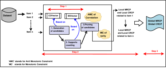
Figure 5.4: Overview of Gmjp when extracting the $\mathcal{RCPR}$ representation.

Data: 1. An extraction context $\mathcal{C}$. 2. A minimal correlation threshold minbond. 3. A minimal conjunctive support threshold minsupp. 4. A specification of the desired result ‘$\mathcal{RCPR}$‘.

Results: The concise exact representation $\mathcal{RCPR}$ = $\mathcal{MRCP}$ $\cup$ $\mathcal{CRCP}$.

Begin  1. Scan the dataset $\mathcal{C}$ twice to build the BSVector and the COVector

for all the items

For each item $I$ $\in$ $\mathcal{I}$

1. $n$ =2;

2. Generate the candidates of size $n$ using the COVector of $I$

2 2

While (The number of the generated candidates is not null) do  i. Prune these candidates w.r.t. the cross-support property

of the bond measure

Prune these candidates w.r.t. the order ideal property

of correlated patterns

Compute the conjunctive and disjunctive supports

and the bond value of the maintained candidates

For each candidate $C$

5

5

5

If (IsCorrelated(C) and IsRare(C)) then

$/*$ Ckeck-Local Minimality of the candidate $C$ $*/$

• Update the set of Local Minimal Rare

Correlated Patterns of size $n$ 6

Find Local Closed Rare Correlated Patterns of size $n$$-$$1$ vi. $n$ = $n$$+$$1$ vii. Generate candidates of size $n$ using the Apriori-Gen

procedure 7  

Find all Global Minimal Rare Correlated Patterns 4. Find all Global Closed Rare Correlated Patterns 5. return $\mathcal{RCPR}$;

8 End

Algorithm 1 Gmjp

9

5.3.2 First Step: The power of the bit vectors and of co-occurrent vectors

Initially, the dataset is scanned in order to extract the items and to build, for each item, the bitset called here “BSVector”. In fact, a bitset is a container that can store a huge number of bits while optimizing the memory consumption (For example, 32 elements are stored in a memory block of 4 bytes). Each block of memory is treated in just one CPU operation by a 32 bits processor. Therefore, we were motivated for these kinds of structures within the Gmjp algorithm in order to optimize the conjunctive and the disjunctive supports computations.

Then, the dataset is scanned again in order to identify, for each item $I$, the list of the co-occurrent items which corresponds to the items occurring in the same transactions as the item $I$. These latter ones are stored in a vector of integers, called here “COVector”. We note that one of the main challenges of the Gmjp algorithm is that it allows pushing two constraints of distinct types and to deliver the output with only two scans of the dataset. We also uphold that the bitsets, when incorporated into the mining process within the Gmjp algorithm, sharply decrease the size of the memory required to store immediate results and significantly save execution costs.

5.3.3 Second Step: Getting the Local Minimal and the Local Closed Rare Correlated Patterns without closure computations

Worth of mention, the main thrust of the Gmjp algorithm is to break the search space into independent sub-spaces. In fact, for each item $I$, a level-wise mining process is performed using the COVector containing the co-occurrent items of $I$. At each level $n$, starting by the second level, a set of candidates is generated, then pruned according to the different pruning strategies described previously. The minimal rare correlated patterns of size $n$, associated to the item $I$, are called Local Minimal Rare Correlated Patterns and they are determined by comparing their bond values versus those of their respective immediate subsets. Similarly, the closed rare correlated patterns of size $n-1$ associated to the item $I$ are called Local Closed Rare Correlated Patterns, and they are determined by comparing their bond values to those of their respective immediate supersets.

It is also important to mention that the implementation of the different stages of this second step (candidate generation, evaluation and pruning) was based on simple vectors of integers. Thus, we do not require more complex data structure during the implementation of the Gmjp algorithm. This feature makes Gmjp a practical approach for handling both monotonic and anti-monotonic constraints even for large datasets.

One of the major challenges in the design of the Gmjp algorithm is how to perform subset and superset checking to efficiently identify Local Minimal and Local Closed patterns$?$ The answer is to construct and manage a multi-map hash structure, ${}^{\textsc{(}}$${}^{\textsc{)}}$ in order to store at each level $n$ the rare correlated patterns of size $n$. This technique has been shown to be very powerful since it makes the subset and the superset checking practical even on dense datasets.

Thus, our proposed efficient solution (as we prove it experimentally later) is to integrate both of the monotonic constraint of rarity and the anti-monotonic constraint of correlation within the mining process and to identify the local closed rare correlated patterns without closure computing.

5.3.4 Third Step: Filtering the Global Minimal and the Global Closed Rare Correlated patterns

After identifying the local minimal and the local closed rare correlated patterns associated to each item $I$ of the dataset $\mathcal{D}$, the third step consists in filtering the $\mathcal{MRCP}$ set of Global Minimal Rare Correlated patterns and the $\mathcal{CRCP}$ set of Global Closed Rare Correlated patterns. This task is performed using two distinct multi-map hash structures. In fact, for each local minimal rare correlated pattern $LM$ previously identified, we check whether it has a direct subset (belonging to the whole set of local minimal patterns) with the same bond value. If it is not the case, then the local minimal pattern $LM$ is a global minimal rare pattern and it is added to the $\mathcal{MRCP}$ set. Similarly, for each local closed rare correlated pattern $LC$ previously identified, we check whether it has a direct superset (belonging to the whole set of local closed patterns) with the same bond value. If it is not the case, then the local closed pattern $LC$ is a global closed rare pattern and it is added to the $\mathcal{CRCP}$ set of Closed rare correlated patterns.

Remark 5

We note that we are limited to the description of the extraction of the $\mathcal{RCPR}$ representation since the post-processing operation of the representations $\mathcal{MM}$ax$\mathcal{CR}$, $\mathcal{M}$in$\mathcal{MCR}$ from the $\mathcal{RCPR}$ representation is obviously done and we prove that the needed execution time is negligible.

In what follows, we illustrate with a running example of the Gmjp algorithm.

5.3.5 Running example

Let us consider the extraction context $\mathcal{C}$ sketched by Table 2.1 (Page 2.1). First, the BSVectors and the COVectors associated to each item of this dataset are constructed, as we plot by Figure 5.5.

Figure 5.5: The BSVectors and the COVectors associated to the items of the extraction context $\mathcal{C}$.

These BSVectors are next used to compute the conjunctive and the disjunctive supports. We have, for example, the item $A$ which belongs to the transactions $\{1,3,5\}$ and the item $C$ which belongs to the transactions $\{1,2,3,5\}$. We, then, have Supp($\wedge$AC) = 3 and Supp($\vee$AC)) = 4.

The local minimal and the local closed correlated rare patterns associated to each item $I$ of the dataset $\mathcal{D}$, are extracted. A detailed example of the process of the item $A$ is given by Figure 5.6.

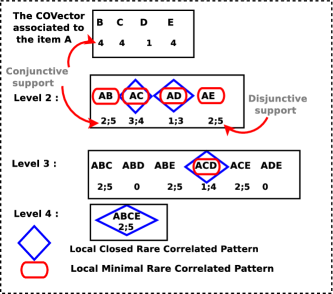
Figure 5.6: Mining Local Minimal and Local Closed Rare Correlated Patterns for the item $A$.

The finally obtained $\mathcal{RCPR}$ representation, for minsupp = 4 and for minbond = 0.20, is composed by the following global minimal and global closed correlated patterns: $\mathcal{RCPR}$ = $\{$ ($A$, $3$, $\displaystyle\frac{3}{3}$), ($D$, $1$, $\displaystyle\frac{1}{1}$), ($AB$, $2$, $\displaystyle\frac{2}{5}$), ($AC$, $3$, $\displaystyle\frac{3}{4}$), ($AD$, $1$, $\displaystyle\frac{1}{3}$), ($AE$, $2$, $\displaystyle\frac{2}{5}$), ($BC$, $3$, $\displaystyle\frac{3}{5}$), ($CD$, $1$, $\displaystyle\frac{1}{4}$), ($CE$, $3$, $\displaystyle\frac{3}{5}$), ($ACD$, $1$, $\displaystyle\frac{1}{4}$), ($BCE$, $3$, $\displaystyle\frac{3}{5}$) and ($ABCE$, $2$, $\displaystyle\frac{2}{5}$)$\}$.

Last, it is important to notice that Gmjp is not an exclusive approach in the sense that it can be coupled with other efficient approaches to mine statistically significant patterns.

In the next section, we present Opt-Gmjp the optimized version of the Gmjp algorithm.

5.4 Opt-Gmjp: The optimized version of Gmjp

In this section, we present Opt-Gmjp the optimized version of Gmjp approach. Our improvements cover the four different scenarios S1, S2, S3 and S4 of the Gmjp approach. Nevertheless, we describe specifically the optimization of the third scenario S3. In fact, the latter deals with two constraints of distinct types namely the anti-monotonic constraint of correlation and the monotonic constraint of rarity.

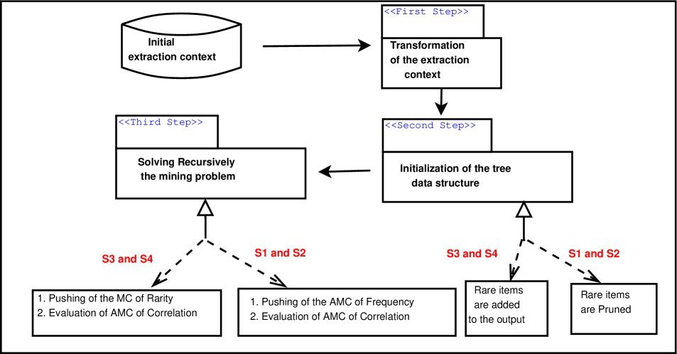
Figure 5.7: An Overview of the Opt-Gmjp algorithm.

We start by presenting a generic overview of the Opt-Gmjp algorithm which is illustrated by Figure 5.7. The pseudo code of Opt-Gmjp, when running the third scenario S3, is given by Algorithm 2 while all of the used notations are illustrated in table 5.1. We note that the “MC“ notation stands for “Monotonic Constraint“ while the “AMC“ notation stands for “Anti-Monotonic Constraint“.

$\mathcal{I}$	:	The set of the distinct items.
$C_{n}$	:	A candidate itemset $C$ of size $n$.
$\mathcal{CAND}_{n}$	:	The Candidate itemsets of size $n$.
$\mathcal{RCP}$	:	The Rare correlated pattern set.

Table 5.1: The notations used within the OptGmjp algorithm.

	A	B	C	D	E
1	$\times$		$\times$	$\times$
2		$\times$	$\times$		$\times$
3	$\times$	$\times$	$\times$		$\times$
4		$\times$			$\times$
5	$\times$	$\times$	$\times$		$\times$

Table 5.2: The Initial extraction context $\mathcal{C}$.

	T1	T2	T3	T4	T5
A	1	0	1	0	1
B	0	1	1	1	1
C	1	1	1	0	1
D	1	0	0	0	0
E	0	1	1	1	1

Table 5.3: The transformed extraction context $\mathcal{C}*$.

In fact, the proposed optimizations are of two types: the transformation of the initial extraction context and the reduction of the number of distinct constraints evaluation. In fact, the measurement of the impact of pushing the monotonic constraint of rarity and the anti-monotonic constraint of correlation early within the Opt-Gmjp algorithm helps to measure the selectivity power of each type of constraint during the mining process.

1. Transformation of the initial extraction context
   Initially, the extraction context is scanned once to build the new transformed extraction context and to construct an in-memory structure (cf. Line 1 Algorithm 2). In fact, we assign to each item a bitset, each column of this bitset indicates the presence or the absence of the item in a specified transaction. For example, if the third column of this list contains 0, then the item $I$ is not present in the third transaction. The transformed extraction context associated to the initial context of Table 5.3 is given by Table 5.3.

2. Initialization of the tree-data structure
   Initially, the $\mathcal{RCP}$ set of rare correlated pattern is set to the empty-set (cf. Line 2 Algorithm 2). Then, we compute the conjunctive support of the items. The items are then sorted in an ascending order of their support (cf. Line 3 Algorithm 2). All the items are added to the nodes of the first level of our tree structure. Thus, they constitute the set of 1-itemsets candidates $\mathcal{CAND}_{1}$ (cf. Line 4 Algorithm 2). All the items are evaluated according to the monotone constraint of rarity: The rare items are printed to the output set, (cf. Line (b) Algorithm 2), while frequent ones are not pruned, i.e., they are maintained.

3. Solving recursively the mining problem
   This step is the main optimization of our algorithm. The idea consists in dividing our mining problem into sub-problems. For each item I, a sub-tree is constructed and a depth-first traversal is therefore performed. The candidates of size $n$ are generated by building intersection of itemsets of size $n-1$ (cf. Line (d) Algorithm 2). They are then evaluated as follows:

   • Evaluation of the anti-monotone constraint of correlation: if the candidate is correlated, we have to distinguish two possible cases:

     • if the candidate is rare correlated, then it is added to the result set (cf. Line (i.1.) Algorithm 2).

     • if the candidate is frequent correlated, then it will not be pruned. In fact, a frequent pattern can have rare supersets. In this case, the candidate is maintained and we continue to develop its sub-tree.

   • if the candidate is not correlated, then all its supersets will not be correlated according to the monotonicity property of the non-correlation constraint. In this case, the candidate and the associated sub-tree are pruned (cf. Line (i.2.) Algorithm 2).

   This generation and evaluation process is continued, the dedicated procedure is recursively called while there is a number of candidates to be generated (cf. Line (g) Algorithm 2). Finally, the used memory is freed and the $\mathcal{RCP}$ is outputted (cf. Line 6 Algorithm 2). The used data structure is illustrated by Figure 5.8.

4. A running Example

   The example shown in Figure 5.8, illustrates how Opt-Gmjp works. The tree is made from five sorted items, D, A, B, C, and E, with their respective supports 1, 3, 4, 4 and 4 respectively. We begin by the node containing the item having the lowest support: which is D. The anti-monotone constraint ’Amc‘ is having the bond value $\geq$ 0.20 and the monotone constraint ’Mc‘ is having the conjunctive support $<$ 4. Intersecting D with A, B, C, and E produces DA, DB, DC and DE. The candidates DB and DE are pruned since they have null support. Thus, their supersets will also have null support. The candidates DA and DC are rare correlated, thus they pass both constraints Amc and Mc. Their intersection produces DAC with support 1 and bond value equal to $\displaystyle\frac{1}{4}$, which also fulfills both constraints. The rare correlated itemsets are added to the output set and the D-sub-tree is deleted from our tree. The A-sub-tree, B-sub-tree, C-sub-tree and E-sub-tree are successively built. The same process is repeated recursively until there’s no more candidates to be generated and evaluated. Finally, the obtained result set of correlated rare itemsets is composed by: ($D$, $1$, $\displaystyle\frac{1}{1}$), ($A$, $3$, $\displaystyle\frac{3}{3}$), ($AB$, $2$, $\displaystyle\frac{2}{5}$), ($AC$, $3$, $\displaystyle\frac{3}{4}$), ($AE$, $2$, $\displaystyle\frac{2}{5}$), ($BC$, $3$, $\displaystyle\frac{3}{5}$), ($CE$, $3$, $\displaystyle\frac{3}{5}$), ($DA$, $1$, $\displaystyle\frac{1}{3}$), ($DC$, $1$, $\displaystyle\frac{1}{4}$), ($ABC$, $2$, $\displaystyle\frac{2}{5}$), ($ABE$, $2$, $\displaystyle\frac{2}{5}$), ($ACE$, $3$, $\displaystyle\frac{3}{4}$), ($BCE$, $3$, $\displaystyle\frac{3}{5}$), ($DAC$, $1$, $\displaystyle\frac{1}{4}$), and ($ABCE$, $2$, $\displaystyle\frac{2}{5}$).

Data: An Extraction Context $\mathcal{C}$, a minimal correlation threshold minbond and a minimal conjunctive support threshold minsupp.

Results: The $\mathcal{RCP}$ set of Rare Correlated Patterns with their respective supports and bond values.

Begin  1. Scan the extraction context $\mathcal{C}$ once to find $\mathcal{I}$ the set of all the distinct items and to build their associated bitsets 2. $\mathcal{RCP}$ := $\emptyset$ 3. Computing the conjunctive support of the items and sorting them in an ascendant order of their support value. 4. $\mathcal{CAND}_{1}$ := $\mathcal{I}$ 5. for each item $I$ $\in$ $\mathcal{I}$ (strating with the item with the lowest support) do (a) Computing the disjunctive support using the bitsets (b) if $I$ is rare then $\mathcal{RCP}$ := $\mathcal{RCP}$ $\cup$ $I$ end if (c) n := 2 (d) $\mathcal{CAND}_{n}$:= generate-Candidate ($\mathcal{CAND}_{n-1}$) $\blacklozenge$ (e) for each candidate $C_{n}$ $\in$ $\mathcal{CAND}_{n}$ do i. if $C_{n}$ is correlated then if $C_{n}$ is rare then (i.1.) $\mathcal{RCP}$ := $\mathcal{RCP}$ $\cup$ $C_{n}$ end if else (i.2.) $\mathcal{CAND}_{n}$ := $\mathcal{CAND}_{n}$ $\backslash$ $C_{n}$ end if end for (f) n := n + 1 (g) Loop to ($\blacklozenge$) while ($\mathcal{CAND}_{n}$ $\neq$ $\emptyset$) end for 6. return $\mathcal{RCP}$ End

Algorithm 2 Opt-Gmjp

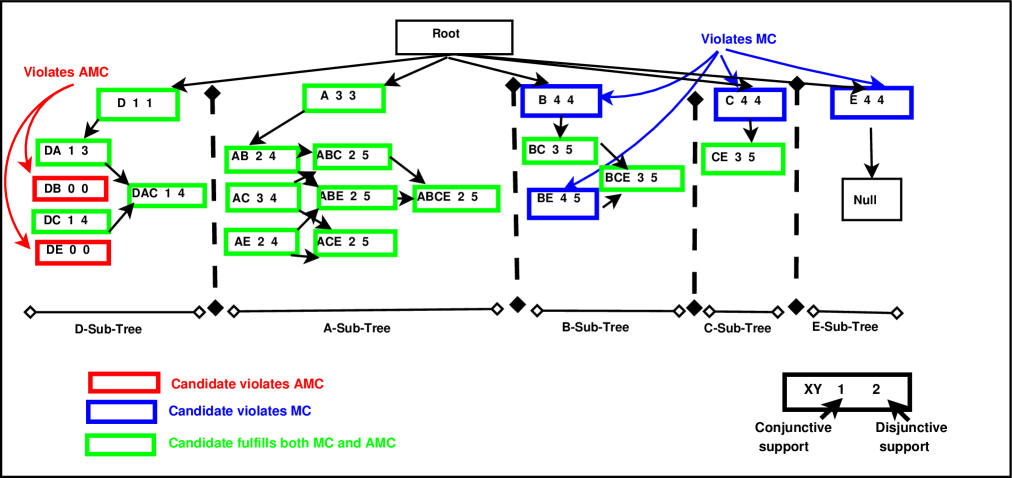
Figure 5.8: The tree data-structure used within the Opt-Gmjp approach and associated to the extraction context given by Table 5.3.

1

In the next section, we present our analysis of the theoretical time complexity of the Gmjp algorithm.

5.5 Theoretical Time Complexity

Proposition 10 gives the theoretical time complexity of the Gmjp algorithm when running the fourth scenario dedicated to the extraction of the $\mathcal{RCPR}$ representation.

Proposition 10

The worst case time complexity of the first step is bounded by $O\textsc{(}N\times M\textsc{)}$, that of the second step is bounded by $O\textsc{(}\textsc{(}N^{3}+\textsc{(}N^{2}\times M\textsc{)}\textsc{)}\times 2^{N}\textsc{)}$, while that of the third step is bounded by $O\textsc{(}N^{2}\textsc{)}$, where $M$ = $|\mathcal{T}|$ and $N$ = $|\mathcal{I}|$. The theoretical complexity in the worst case of the Gmjp algorithm is bounded by the sum of those of its three steps.

Proof. First of all, let us recall the respective roles of the distinct steps of the Gmjp algorithm.

• The first step: Scanning the extraction context twice in order to build the bitset vector and the co-occurring vector associated to each item $I$.
  The complexity $\mathcal{C}_{{}_{1}}$ of this step, is equal to, $\mathcal{C}_{{}_{1}}$ = 2 $\times$ $O\textsc{(}N\times M\textsc{)}$ $\approx$ $O\textsc{(}N\times M\textsc{)}$.

• The second step: Extracting the local minimal and the local closed rare correlated patterns.
  The cost of this step is equal to those of its associated instructions which are as follows:

  1. The cost of the initialization of the integer $n$ carried out in line (a) (cf. Algorithm 1) is in $O\textsc{(}1\textsc{)}$.

  2. The generation of the candidates of size $n$, (cf. line (b) in Algorithm 1), is done in $O\textsc{(}N-1\textsc{)}$ since in the worst case the number of generated candidates is $N-1$.

  3. The cost of the pruning of candidates w.r.t. the cross-support property of the bond measure is done in $O\textsc{(}N^{2}\textsc{)}$ (cf. line (i) in Algorithm 1).

  4. The cost of the pruning of candidates w.r.t. the ideal order property of correlated patterns is done in $O\textsc{(}N^{2}\textsc{)}$ (cf. line (ii) in Algorithm 1).

  5. The cost of the computation of the conjunctive and the disjunctive supports of the itemset candidates is bounded by $O\textsc{(}N\times M\textsc{)}$ (cf. line (iii) in Algorithm 1).

  6. The checking of the constraints of rarity and of correlation is done in $O\textsc{(}1\textsc{)}$, while the checking of the local minimality of the set of candidates is done in $O\textsc{(}N^{2}\textsc{)}$ and the updating of the $\mathcal{MRCP}$ set of minimal rare correlated patterns is done in $O\textsc{(}1\textsc{)}$ (cf. line (iv) in Algorithm 1).

  7. The extraction of the local closed rare correlated patterns of size $n-1$ is bounded by $O\textsc{(}N^{2}\textsc{)}$ (cf. line (v) in Algorithm 1).

  8. The cost of increasing the integer $n$ is done in $O\textsc{(}1\textsc{)}$ (cf. line (vi) in Algorithm 1).

  9. There are, in the worst case, $\textsc{(}2^{N}-N-1\textsc{)}$ candidates to be generated using the Apriori-Gen procedure (cf. line (vii) in Algorithm 1). The cost of this step is bounded by $O\textsc{(}2^{N}-N\textsc{)}$.

  Consequently, the cost $\mathcal{C}_{{}_{2}}$ of this second step, is approximatively equal to:

  $\mathcal{C}_{{}_{2}}$ = $O\textsc{(}1\textsc{)}$ $+$ $O$($N$ - $1$) $\times$ [ $O$($2^{N}$ - $N$) $\times$ [ $O\textsc{(}N^{2}\textsc{)}$ $+$ $O\textsc{(}N^{2}\textsc{)}$ $+$ $O\textsc{(}N\times M\textsc{)}$ $+$ $O\textsc{(}1\textsc{)}$ $+$ $O\textsc{(}N^{2}\textsc{)}$ $+$ $O\textsc{(}1\textsc{)}$ $+$ $O\textsc{(}N^{2}\textsc{)}$ $+$ $O\textsc{(}1\textsc{)}$ ]]

  $\approx$ $O\textsc{(}1\textsc{)}$ $+$ $O$($N$ - $1$) $\times$ [ $O$($2^{N}$) $\times$ [ $O\textsc{(}N^{2}\textsc{)}$ $+$ $O\textsc{(}N\times M\textsc{)}$ ] ]

  $\approx$ $O$($2^{N}$) $\times$ ( $O\textsc{(}N^{3}\textsc{)}$ $+$ $O\textsc{(}N^{2}\times M\textsc{)}$)

  $\approx$ $O$(($N^{3}$ + ($N^{2}$ $\times$ $M$)) $\times$ $2^{N}$).

• The third step: Filtering the global minimal and the global closed patterns among the local ones.

  In fact, this step consists in checking for each local minimal (resp. closed) pattern, whether it has a subset (resp. superset) with the same bond value or not. The complexity, $\mathcal{C}_{{}_{3}}$, of this step is then bounded by $O\textsc{(}N^{2}\textsc{)}$ (cf. lines $3$ and $4$ in Algorithm 1).

Consequently, the complexity of the Gmjp algorithm is equal to: $\mathcal{C}_{{}_{1}}$ $+$ $\mathcal{C}_{{}_{2}}$ $+$ $\mathcal{C}_{{}_{3}}$

$\approx$ $O{\textsc{(}}N\times M\textsc{)}$ $+$ $O$(($N^{3}$ + ($N^{2}$ $\times$ $M$)) $\times$ $2^{N}$) $+$ $O\textsc{(}N^{2}\textsc{)}$

$\approx$ $O$(($N^{3}$ + ($N^{2}$ $\times$ $M$)) $\times$ $2^{N}$) $\approx$ $2^{N}$.

It is important to mention that the complexity in the worst case of the Gmjp algorithm is not reachable in practice. Indeed, there is not a context that simultaneously gives the respective worst case complexities of the three steps. Hence, the worst case complexity of Gmjp is roughly bounded by the sum of those of its three steps.

In the next section, we describe the query process of the $\mathcal{RCPR}$ representation and the regeneration of the $\mathcal{RCP}$ set from the $\mathcal{RCPR}$ representation.

5.6 The query and the regeneration strategies

We begin the first sub-section with the querying strategy of the $\mathcal{RCPR}$ representation.

5.6.1 Querying of the $\mathcal{RCPR}$ representation

In the following, we introduce the Regenerate algorithm, whose pseudo code is given by Algorithm 3, dedicated to the query of the $\mathcal{RCPR}$ representation. In fact, the interrogation of the $\mathcal{RCPR}$ representation allows determining the nature of a given pattern. If it is a rare correlated pattern, then, its conjunctive, disjunctive, negative supports as well as its bond value are faithfully derived from the $\mathcal{RCPR}$ representation.

$\bullet$ Description of the Regenerate algorithm

The Regenerate algorithm takes as an input the number of the transactions $|\mathcal{T}|$, the $\mathcal{RCPR}$ representation and an arbitrary itemset $I$ and it proceeds in two distinct ways depending on the state of $I$:

• If the itemset $I$ belong to the $\mathcal{RCPR}$ representation (cf. Line 2 Algorithm 3), then $I$ is a rare correlated itemset. In this regard, we have the conjunctive support and the bond values, thus we compute the disjunctive and the negative supports. The disjunctive support is equal to the ratio of the conjunctive support by the bond value, (cf. Line 3 Algorithm 3). The negative support is equal to the number of transactions $|\mathcal{T}|$ minus the disjunctive support (cf. Line 4 Algorithm 3). The algorithm returns the values of the different supports as well as the bond value of the rare correlated itemset $I$, (cf. Line 5 Algorithm 3).

• If the itemset $I$ do not belong to the $\mathcal{RCPR}$ representation, then we distinguish two different cases:

  • If it exists two itemsets $J$ and $Z$ belonging to $\mathcal{RCPR}$ such as, $J$ $\subset$ $I$ and $Z$ $\supset$ $I$, (cf. Line 7 Algorithm 3), then $I$ is a rare correlated pattern and we have to determine its supports and correlation values. The closed itemset $F$ associated to $I$ is the minimal itemset, according to the inclusion set, that covers $I$; (cf. Line 9 Algorithm 3). The conjunctive support and the bond value of $I$ are equal to those of its closure $F$, (cf. Lines 10 and 11 Algorithm 3). The disjunctive and the supports are computed in the same manner as the first case, (cf. Lines 12 and 13 Algorithm 3). Finally the algorithm outputs the values of the different supports as well as the bond value of the rare correlated itemset $I$, (cf. Line 14 Algorithm 3).

  • If it not exists two itemsets $J$ and $Z$ belonging to $\mathcal{RCPR}$ such as, $J$ $\subset$ $I$ and $Z$ $\supset$ $I$, then the algorithm outputs the emptyset to indicates that the itemset $I$ is not a rare correlated pattern, (cf. Line 16 Algorithm 3).

Data:

1. An arbitrary pattern $I$.

2. $\mid$$\mathcal{T}$$\mid$: The number of transactions.

3. The $\mathcal{RCPR}$ representation = $\mathcal{MRCP}$ $\cup$ $\mathcal{CRCP}$.

Results: The conjunctive, disjunctive, negative supports and the bond value of the pattern $I$ if it is rare correlated, the empty set otherwise.

Begin  If ($I$ $\in$ $\mathcal{RCPR}$) then  Supp($\vee$$I$) = $\displaystyle\frac{\displaystyle Supp\textsc{(}\wedge I\textsc{)}}{\displaystyle\textit{bond}\textsc{(}I\textsc{)}}$ ;

Supp($\neg$$I$) = $\mid$$\mathcal{T}$$\mid$ $-$ Supp($\vee$$I$) ;

return $\{$$I$, Supp($\wedge$$I$), Supp($\vee$$I$), Supp($\neg$$I$), bond($I$)$\}$ ;

 Else  If ($\exists$ $J$, $Z$ $\in$ $\mathcal{RCPR}$ $\mid$ $J$ $\subset$ $I$ and $I$ $\subset$ $Z$) then  $/*$ $F$ is the closed pattern associated to the candidate $I$ $*/$

$F$:= $\min_{\subseteq}$$\{$$I_{1}$ $\in$ $\mathcal{RCPR}$ $\mid$ $I$ $\subset$ $I_{1}$$\}$ ;

Supp($\wedge$$I$) = Supp($\wedge$$F$);

bond($I$) = bond($F$);

Supp($\vee$$I$) = $\displaystyle\frac{\displaystyle Supp\textsc{(}\wedge I\textsc{)}}{\displaystyle\textit{bond}\textsc{(}I\textsc{)}}$;

Supp($\neg$$I$) = $\mid$$\mathcal{T}$$\mid$ $-$ Supp($\vee$$I$);

return $\{$$I$, Supp($\wedge$$I$), Supp($\vee$$I$), Supp($\neg$$I$), bond($I$)$\}$ ;

  Else  return $\emptyset$;

    End

Algorithm 3 Regenerate

Example 31

Let us consider the $\mathcal{RCPR}$ representation given by Example 19, (Page 19), for minsupp = 4 and minbond = 0.2. Consider the pattern $ACE$. When comparing the pattern $ACE$ with the elements of the $\mathcal{RCPR}$ representation, we remark that $AE$ $\subset$ $ACE$ and $ACE$ $\subset$ $ABCE$. Then, the pattern $ACE$ is a rare correlated pattern and the associated closed pattern is $ABCE$. Consequently, Supp($\wedge$$ACE$) = Supp($\wedge$$ABCE$) = 2, Supp($\vee$$ACE$) = Supp($\vee$$ABCE$) = 5, Supp($\neg$$ACE$) = $|\mathcal{T}|$ - Supp($\vee$$ACE$) = 5 - 5 = 0 and bond($ACE$) = bond($ABCE$) = $\displaystyle\frac{2}{5}$. Consider the pattern $BE$. In fact, $BE$ $\notin$ $\mathcal{RCPR}$ and there is no element of $\mathcal{RCPR}$ which is included in $BE$. Therefore, the Regenerate algorithm returns the empty set and indicates that the pattern $BE$ is not a rare correlated pattern.

In what follows, we introduce the strategy of regeneration of the $\mathcal{RCP}$ set, i.e. the set of all rare correlated patterns, from this representation.

20

20

20

20

20

20

20

20

20

20

20

20

20

20

20

20

20

20

20

20

5.6.2 Regeneration of the $\mathcal{RCP}$ set from the $\mathcal{RCPR}$ representation

The regeneration of the $\mathcal{RCP}$ set from the $\mathcal{RCPR}$ representation is achieved through the RcpRegeneration algorithm which pseudo-code is given by Algorithm 4. This latter algorithm inputs the $\mathcal{RCPR}$ representation and provides the $\mathcal{RCP}$ set of rare correlated patterns. The conjunctive support and the bond value of each pattern are exactly determined.

$\bullet$ Description of the RcpRegeneration algorithm

The RcpRegeneration algorithm takes as an input the number of the transactions $|\mathcal{T}|$ and the $\mathcal{RCPR}$ representation which is composed by the two sets $\mathcal{MRCP}$ and $\mathcal{CRCP}$. The algorithm generates the $\mathcal{RCP}$ set as described in the following:

1. Initially, the $\mathcal{RCP}$ set is assigned with the empty set, (cf. Line 2 Algorithm 4). Then, all the itemsets of the $\mathcal{RCPR}$ representation (The elements of the $\mathcal{MRCP}$ and the $\mathcal{CRCP}$ sets) are added to the $\mathcal{RCP}$ set, (cf. Lines 4 and 5 Algorithm 4).

2. For each minimal generator $M$ of the $\mathcal{MRCP}$ set, we determine its closure $F$ among the $\mathcal{CRCP}$ set. In fact, $F$ corresponds to the minimal itemset, according to inclusion set, that covers $M$ (cf. Line 9 Algorithm 4).

3. At this step, we derive all the patterns that are included between the minimal generator $M$ and its closure $F$. Thus, we need an intermediate itemset $D$ that contains the set of items belonging to $F$ and not to $M$: $D$ = $F$$\backslash$$M$, (cf. Line 11 Algorithm 4). Then, each item $j$ included in the itemset $D$, is concatenated with the generator $M$ in order to form a new itemset $X$: $X$ = $M$ $\cup$ $j$, (cf. Line 13 Algorithm 4). The conjunctive support and the bond value of $X$ are equal to those of its closure $F$ (cf. Lines 14 and 15 Algorithm 4).

4. Finally, the rare correlated itemset $X$ is added to the $\mathcal{RCP}$ set after the non-redundancy checking (cf. Line 18 Algorithm 4). The whole $\mathcal{RCP}$ set is outputted in Line 19 of algorithm 4.

Data: 1. The $\mathcal{RCPR}$ representation = $\mathcal{MRCP}$ $\cup$ $\mathcal{CRCP}$. 2. The number of transactions: $|$$\mathcal{T}$$|$.

Results: The $\mathcal{RCP}$ set of rare correlated patterns.

Begin  $\mathcal{RCP}$:= $\emptyset$;

$/*$ The elements of $\mathcal{RCPR}$ are appended to the $\mathcal{RCP}$ set $*/$

for ($M\in\mathcal{RCPR}$) do  $\mathcal{RCP}$:= $\mathcal{RCP}$ $\cup$ $\{$$M$, Supp($\wedge$$M$), bond($M$)$\}$ ;

  $/*$ Process of each element $M$ of $\mathcal{MRCP}$ separately $*/$

for ($M\in\mathcal{MRCP}$) do  $/*$ Identification of the closed pattern associated to the minimal $M$ $*/$

$F$:= $\min_{\subseteq}$$\{$$M_{1}$ $\in$ $\mathcal{CRCP}$ $\mid$ $M$ $\subset$ $M_{1}$$\}$;

$/*$ Derivation of the rare correlated patterns included between $M$ and $F$ $*/$

$D$:= $F$ $\backslash$ $\{{i}$, $\forall$ ${i}$ $\in$ $M$$\}$

for ($j$ $|$ $j$ $\in$ $D$) do  for ($X$ $\mid$ $X$ = $M$ $\cup$ ${j}$ ) do 

Supp($\wedge$$X$) = Supp($\wedge$$F$);

bond($X$) = bond($F$) ;

$/*$ Check of the uniqueness of the elements of the $\mathcal{RCP}$ set $*/$

If ($X$ $\notin$ $\mathcal{RCP}$) then  $\mathcal{RCP}$:= $\mathcal{RCP}$ $\cup$ $\{$$X$, Supp($\wedge$$X$), bond($X$)$\}$ ;

    return $\mathcal{RCP}$;

End

Algorithm 4 RcpRegeneration

17

17

17

17

17

17

17

17

17

17

17

17

17

17

17

17

17

Example 32

Consider the $\mathcal{RCPR}$ representation illustrated by example 19 , (Page 19), for minsupp = 4 and minbond = 0.2. The regeneration of the $\mathcal{RCP}$ set is carried out as follows. Firstly, the $\mathcal{RCP}$ set is initialized to the empty set. Then, the elements of the $\mathcal{RCPR}$ representation are appended to the $\mathcal{RCP}$ set. We have so, $\mathcal{RCP}$ = $\{$($A$, $3$, $\displaystyle\frac{3}{3}$), ($D$, $1$, $\displaystyle\frac{1}{1}$), ($AB$, $2$, $\displaystyle\frac{2}{5}$), ($AC$, $3$, $\displaystyle\frac{3}{4}$), ($AD$, $1$, $\displaystyle\frac{1}{3}$), ($AE$, $2$, $\displaystyle\frac{2}{5}$), ($BC$, $3$, $\displaystyle\frac{3}{5}$), ($CD$, $1$, $\displaystyle\frac{1}{4}$), ($CE$, $3$, $\displaystyle\frac{3}{5}$), ($ACD$, $1$, $\displaystyle\frac{1}{4}$), ($BCE$, $3$, $\displaystyle\frac{3}{5}$), ($ABCE$, $2$, $\displaystyle\frac{2}{5}$)$\}$. Then, the patterns $ABE$ and $ABC$ included between the minimal pattern ($AB$, 2, $\displaystyle\frac{2}{5}$) and its closure ($ABCE$, 2, $\displaystyle\frac{2}{5}$) are generated. In addition, the pattern $ACE$, included between the minimal pattern ($AE$, 2, $\displaystyle\frac{2}{5}$) and its closure ($ABCE$, 2, $\displaystyle\frac{2}{5}$), is also derived. The patterns $ABE$, $ABC$ and $ACE$ are also generated, as they share the same conjunctive support and bond value of the closed pattern $ABCE$, are then inserted in the $\mathcal{RCP}$ set. This latter is updated and contains all the rare correlated patterns: $\mathcal{RCP}$ = $\{$($A$, $3$, $\displaystyle\frac{3}{3}$), ($D$, 1, $\displaystyle\frac{1}{1}$), ($AB$, $2$, $\displaystyle\frac{2}{5}$), ($AC$, $3$, $\displaystyle\frac{3}{4}$), ($AD$, 1, $\displaystyle\frac{1}{3}$), ($AE$, $2$, $\displaystyle\frac{2}{5}$), ($BC$, $3$, $\displaystyle\frac{3}{5}$), ($CD$, 1, $\displaystyle\frac{1}{4}$), ($CE$, $3$, $\displaystyle\frac{3}{5}$), ($ABC$, 2, $\displaystyle\frac{2}{5}$), ($ABE$, 2, $\displaystyle\frac{2}{5}$), ($ACD$, 1, $\displaystyle\frac{1}{4}$), ($ACE$, 2, $\displaystyle\frac{2}{5}$), ($ABCE$, 2, $\displaystyle\frac{2}{5}$)$\}$.

5.7 Conclusion

We introduced, in this chapter, the Gmjp extraction approach to mine correlated patterns in a generic way (i.e., with two types of constraints: anti-monotonic constraint of frequency and monotonic constraint of rarity). Our approach is based on the key notion of bitsets codification that supports efficient correlated patterns computation thanks to an adequate condensed representation of patterns. In the next chapter, we present our experimental evaluation of Gmjp and of Opt-Gmjp according to both quantitative and qualitative aspects.

Part III Experiments and Classification Process

Chapter 6 Experimental Validation

6.1 Introduction

This chapter is devoted to the experimental evaluation of the proposed Gmjp algorithm. Our evaluation is performed on two principal axes. In Section 6.2, we present the experimental environment, specifically the characteristics of the used datasets as well as the experimental protocol. Then, we present in Section 6.3 the qualitative evaluation of the proposed condensed representations which is measured by the compactness rates offered by each proposed exact and approximate concise representation. Section 6.4, is dedicated to the evaluation of the performance of both Gmjp, as well as the optimized version that highlights the important measured improvements.

6.2 Experimental Environment

In this chapter, we aim to show, through extensive carried out experiments, that the different proposed concise representations provide interesting compactness rates compared to the whole set of correlated patterns. In addition to this, we aim to prove the efficiency of the proposed Gmjp approach. In our experiments, we used two evaluation measures: the conjunctive support to measure the frequency (respectively the rarity) and the bond measure to evaluate the correlation of a pattern.

All experiments were carried out on a PC equipped with a $2.4$ GHz Intel Core TM i3 processor and $4$ GB of main memory, running the Linux Ubuntu 12.04. The used datasets are described in what follows.

6.2.1 Datasets

The experiments were carried out on different dense and sparse benchmark datasets ${}^{\textsc{(}}$${}^{\textsc{)}}$. Table 6.1 summarizes the characteristics of the considered datasets. A brief description of the content of each dataset is given below:

• Connect: This dataset contains all legal positions in the game of connect-4 in which neither player has won yet, and in which the next move is not forced.

• Mushroom: This dataset includes descriptions of hypothetical samples corresponding to 23 species of gilled mushrooms.

• Pumsb: This dataset contains Census Data from PUMS (Public Use Microdata Samples). Each object represents the answers to a census questionnaire.

• Pumsb*: This dataset is obtained after deleting all frequent items for a minimum support threshold set to 80$\%$ in the original Pumsb.

• Retail: The Retail dataset contains information about Market Basket of clients in a Belgian Supermarket.

• Accidents: This dataset represents traffic accidents obtained from the National Institute of Statistics (NIS) for the Region of Flanders (Belgium).

• T10I4D100K: This is a synthetic dataset generated using the generator from the IBM Almaden Quest Research Group. The goal of this generator is to create objects similar to those obtained in a supermarket environment.

• T40I10D100K: Identically to T10I4D100K, this dataset is also generated from the IBM generator. The differences between this dataset and T10I4D100K are the number of items and the average size of the objects.

Dataset	Property	Number	Number of	Average length
		of items	transactions	of transactions
Connect	Dense	129	67, 557	43.00
Chess	Dense	75	3 196	37.00
Mushroom	Dense	119	8, 124	23.00
Pumsb	Dense	7, 117	49, 046	74.00
Pumsb*	Dense	7, 117	49, 046	50.00
Retail	Sparse	16, 470	88, 162	10.00
Accidents	Sparse	468	340, 183	33.81
T10I4D100K	Sparse	870	100, 000	10.10
T40I10D100K	Sparse	942	100, 000	39.61

Table 6.1: Characteristics of the benchmark datasets.

6.2.2 Experimental Protocol

Our objective is to prove, through extensive carried out experiments, the efficiency of the proposed Gmjp algorithm.

✓Our first batch of experiments focus on evaluating the compactness rates by different condensed representations of rare correlated patterns. We also build a quantitative comparison between the $\mathcal{FCP}$, the $\mathcal{RCP}$ sets and their associated condensed representations.

✓Our second batch of experiments focus on studying running times of the proposed Gmjp algorithm while running the four different scenarios.

6.3 Evaluation of the compactness rates offered by the proposed representations

The compactness rate offered by a concise representation measures the reduction of the size of the representation compared to the size of the whole set of patterns. For example, for the $\mathcal{RCPR}$ representation, the compactness rate is equal to: 1 - $\frac{|\mathcal{RCPR}|}{|\mathcal{RCP}|}$. Worth of cite, our experimental study confirms that the $\mathcal{RCPR}$ representation is a perfect cover of the $\mathcal{RCP}$ set. In fact, the obtained results show that the size of $\mathcal{RCPR}$ is always smaller than that of the $\mathcal{RCP}$ set over the entire range of the considered support and bond thresholds. Our study concerns both dense and sparse datasets.

6.3.1 Effect of minsupp variation

For example, considering the Mushroom dataset for minsupp = 35$\%$ and minbond = 0.15: $|\mathcal{RCPR}|$ = 1, 810 while $|\mathcal{RCP}|$ = 100, 156, with a reduction rate reaching approximately 98$\%$. This is explained by the nature of the induced equivalence classes. In fact, we have in this case, $|\mathcal{MRCP}|$ = 1, 412 and $|\mathcal{CRCP}|$ = 652. Since the $\mathcal{RCPR}$ representation corresponds to the union without redundancy of the $\mathcal{MRCP}$ and the $\mathcal{CRCP}$ sets, we have always $|\mathcal{RCPR}|$ $\leq$ $|\mathcal{MRCP}|$ + $|\mathcal{CRCP}|$.

In this respect, Figure 6.1 shows that all the compression rates proportionally vary to minsupp and disproportionately with respect to minbond values. This is due to the fact that, the size of the different representations increases as far as minsupp increases and decreases whenever minbond increases.

Figure 6.1: Sizes of the different representations when minsupp varies and minbond is fixed.

We also find that the respective sizes of the concise exact representations $\mathcal{MM}$$ax$$\mathcal{CR}$ and $\mathcal{M}$$in$$\mathcal{MCR}$ never exceed the size of the $\mathcal{RCPR}$ representation. This is justified by the nature of the elements composing both representations. In fact, the $\mathcal{MM}$$ax$$\mathcal{CR}$ is composed by the $\mathcal{MRCP}$ set of minimal rare correlated patterns and the $\mathcal{M}ax$$\mathcal{CRCP}$ set of maximal closed rare correlated patterns. Nevertheless, we confirm that the size of the $\mathcal{M}ax$$\mathcal{CRCP}$ set is always lower than that of the $\mathcal{CRCP}$ set. According to the $\mathcal{M}$$in$$\mathcal{MCR}$ representation, it is based on the $\mathcal{M}in$$\mathcal{MRCP}$ set of the minimal elements of the $\mathcal{MRCP}$ set and on the $\mathcal{CRCP}$ set. In fact, we remark that the size of the $\mathcal{M}in$$\mathcal{MRCP}$ set never exceeds the size of the $\mathcal{MRCP}$ set.

In what follows, we evaluate the compactness of the representations based on the variation of the correlation threshold minbond.

6.3.2 Effect of minbond variation

Let us consider the results depicted by Figure 6.2. The first intuition is that all the compression rates vary disproportionately to minbond values. For the Pumsb* dataset, for minsupp = 80$\%$ and for minbond = 0.30, we have $|\mathcal{RCP}|$ = 65, 536 $>$ $|\mathcal{RCPR}|$ $=$ $|$$\mathcal{RMM}$$ax$$\mathcal{F}|$ $=$ $|\mathcal{M}in$$\mathcal{MRCP}|$ = 2, 048. Now, while increasing minbond from 0.30 to 0.60, we remark that the size of the $\mathcal{RCP}$ increase as well the $|\mathcal{RCPR}|$ representation, whereas the size of $\mathcal{RMM}$$ax$$\mathcal{F}$ and of $\mathcal{M}in$$\mathcal{MRCP}$ are unchanged. Thus, these representations offer constant reduction rates in spite of minbond variation. For the same example, we have $|\mathcal{RCP}|$ = 130, 000 $>$ $|\mathcal{RCPR}|$ = 4, 096 $>$ $|$$\mathcal{RMM}$$ax$$\mathcal{F}|$ = 2, 048 $=$ $|\mathcal{M}in$$\mathcal{MRCP}|$ = 2, 048.

Figure 6.2: Sizes of the different representations when minbond varies and minsupp is fixed.

We sketch in Table 6.2, the experimental results associated to both the $\mathcal{FCP}$ set of frequent correlated patterns and to the $\mathcal{RCP}$ set of rare correlated patterns. To summarize, the concise representations $\mathcal{FCCPR}$ and $\mathcal{RCPR}$ present very encouraging reduction rates over several datasets and for different ranges of minsupp and minbond thresholds. We note that, the ‘gain‘ corresponds to the “reduction rate“ said also “compactness rate“.

Dataset	minsupp	minbond	$\#$ $\mathcal{FCP}$	$\#$ $\mathcal{FCCPR}$	Gain of		$\#$ $\mathcal{RCP}$	$\#$ $\mathcal{RCPR}$		Gain of
					$\mathcal{FCCPR}$					$\mathcal{RCPR}$
Mushroom	30$\%$	0.15	2, 701	427	84.19$\%$		98, 566	1, 704		98.27$\%$
	45$\%$	0.15	307	83	72.96$\%$		100, 960	1, 985		98.03$\%$
Pumsb*	40$\%$	0.45	10, 674	1646	84.57$\%$		448, 318	3, 353		99.25$\%$
	40$\%$	0.50	9, 760	1325	86.42$\%$		82, 413	3, 012		96.34$\%$
Connect	10$\%$	0.80	534, 026	15, 152	97.16$\%$		56	56		0$\%$
	50$\%$	0.80	533, 991	15, 117	97.16$\%$		91	91		0$\%$
Accidents	40$\%$	0.30	32, 529	32, 528	0$\%$		117, 805	1, 722		98.53$\%$
	60$\%$	0.30	2, 057	2, 047	0$\%$		148, 259	2, 743		98.14$\%$

Table 6.2: Compactness Rates associated to the $\mathcal{FCP}$ set vs. the $\mathcal{RCP}$ set.

At this stage, we have analyzed the variation of the size of the different concise exact representations according to both minsupp and minbond variations. In the next section, we put the focus on the evaluation of the running time of the proposed Gmjp approach.

6.4 Evaluation of the running time of Gmjp

6.4.1 Overall Performance Evaluation of Gmjp

We emphasize that, according to the results given by Table 6.3 ${}^{\textsc{(}}$${}^{\textsc{)}}$ , that the execution time varies depending on the number of distinct items of the considered dataset. This is explained by the principle of Gmjp which is based on the idea of processing each item separately and based on the list of the co-occurrent of each item.

For example, the computation costs are relatively high for the T40I10D100K dataset, and they are low for the Mushroom dataset. This is explained by the fact that, the Mushroom dataset only contains 119 items while the T40I10D100K dataset contains 942 items. We also note that the highest execution times are obtained with the Retail dataset, since this latter contains a high number of distinct items, equal to 16, 470.

Dataset	Number	Average	Average	Average	Average	Average	Average
	of Items	minsupp	minbond	Time S1	Time S2	Time S3	Time S4
Mushroom	119	58$\%$	0.30	7	11.4	20	19.6
		40$\%$	0.57	3.75	5.25	11	709
Accidents	468	7.8$\%$	0.50	709	703	793	784.2
Retail	16, 470	25.83$\%$	0.50	5.83	13.16	1903	1902
T10I4D100K	870	5$\%$	0.20	2	3	163	163
T40I10D100K	942	8.2$\%$	0.50	148	182.6	491	490.4

Table 6.3: Performance Analysis of Gmjp on UCI benchmarks (Time in seconds).

It is worth of mention that the computation time of the fourth scenario dedicated to the extraction of the $\mathcal{RCPR}$ representation are the highest ones among the other scenarios. This can be explained by the fact that the extraction of the $\mathcal{RCPR}$ representation is the most complex mining task within the Gmjp approach. Thereby, we focus on the next subsection on studying the cost of the three different steps of Gmjp when extracting the $\mathcal{RCPR}$ representation.

6.4.2 Performance Evaluation of the $\mathcal{RCPR}$ representation Mining

We study, in this subsection, the running time of need for the extraction of the $\mathcal{RCPR}$ representation. It is worth noting that the running times of the Gmjp algorithm vary according to the characteristics of the dataset. For example, the computation costs are relatively high for the T10I10D100K dataset, and they are low for the Mushroom dataset. This is due to the difference in the characteristics of these two datasets. In fact, the Mushroom dataset only contains 119 items and 8, 124 transactions while the T10I10D100K dataset contains 870 items and 100, 000 transactions. We also note, for the different datasets, that the extraction costs are slightly sensitive to the changes of the minsupp and minbond values.

We present, in Tables 6.4 and 6.5, the CPU time corresponding to each step of the Gmjp algorithm and depending respectively on the variation of minsupp and on the variation of minbond.

Dataset	minbond	minsupp	First Step	Second Step	Third Step
Mushroom	0.3	20$\%$	6	13	0
		40$\%$	6	13	0
		60$\%$	6	14	0
		80$\%$	6	15	0
Retail	0.5	5$\%$	276	1, 627	0
		10$\%$	273	1, 627	0
		30$\%$	274	1, 628	0
		50$\%$	275	1, 628	0
Accidents	0.5	1$\%$	724	67	0
		3$\%$	714	67	0
		5$\%$	716	67	0
		10$\%$	715	67	0
		15$\%$	717	67	0
		20$\%$	717	67	0

Table 6.4: Impact of the variation of minsupp, for the three steps of the Gmjp algorithm (Time in seconds).

We conclude, according to these results, that the obtained execution times are slightly sensitive to the variation of the minbond and minsupp values.

Dataset	minsupp	minbond	First Step	Second Step	Third Step
Mushroom	50$\%$	0.4	6	4	0
		0.7	6	1	0
		1	6	1	0
T10I4D100K	5$\%$	0.2	25	137	0
		0.4	26	138	0
		0.6	26	138	0
		0.8	25	138	0
		1	25	137	0

Table 6.5: Impact of the variation of minbond, for the three steps of the Gmjp algorithm (Time in seconds).

We have, for example, the CPU time needed for the execution of the first step for the T10I4D100K dataset is about 26 seconds, while for the Retail dataset, the execution of the first step needs about 275 seconds. This is justified by the fact that the T10I4D100K dataset contains only 870 items while the Retail dataset contains 16, 470 items. We also remark, for the Accidents dataset, that the execution times are relatively high compared to the other datasets. This is justified by its high number of transactions, equal to 340, 183 transactions which induces that the first step becomes more costly. In this regard, the first step of the building of the BSVector and the COVector of the items needs about 720 seconds and it lasts more than the second step, which needs only 67 seconds.

It is also important to mention that the CPU time dedicated to the third step, allowing to filter the global minimal and the global closed patterns among the sets of the identified local minimal and local closed ones, is negligible and equal to null. This confirms the very good choice of the suitable multimap data structures during the third step.

We also note, that the execution times needed for the post-processing of the representations $\mathcal{MM}$ax$\mathcal{CR}$, $\mathcal{M}$in$\mathcal{MCR}$ from the $\mathcal{RCPR}$ representation are negligible.

We have, thus, evaluated the performance of the Gmjp approach while running the four different execution scenarios. We focused specially on the fourth scenario dedicated to the extraction of the $\mathcal{RCPR}$ representation. In the next section, we evaluate Opt-Gmjp the optimized version of the Gmjp approach.

6.5 Optimizations and Evaluations

Our aim in the next subsections is to evaluate the impact of varying the thresholds of both the correlation and the rarity constraints.

In the remainder, we study the impact of the rarity constraint threshold variation on the execution time of the Opt-Gmjp version.

6.5.1 Effect of minsupp variation

Table 6.6 presents our results while fixing the minbond threshold and varying the monotone constraint of rarity threshold, minsupp. We consider as an example the Mushroom dataset, while varying minsupp from 20$\%$ to 80$\%$, the size of the result set |$\mathcal{RCP}$| varies from 261 itemsets to 3352 itemsets while the CPU-time and the memory consumption underwent a slight variation. Whereas, for the T40I10D100K dataset, the variation of minsupp from 2$\%$ to 15$\%$ induces an increase in the CPU-time of the second and third steps from 60.09 to 79.49 seconds. The size of the output result increase also from 341 to 932 itemsets.

The Chess dataset presents a specific behavior according to minsupp variation. The variation of minsupp from 30$\%$ to 50$\%$ induces an increase in the CPU-time of the second and third steps from 5.604 to 300.163 seconds. The size of the $\mathcal{RCP}$ set increase in a very significant way from 618 to 36010, 648 itemsets.

6.5.2 Effect of minbond variation

Table 6.7 presents the results obtained when varying the correlation threshold minbond for a fixed minsupp threshold. In this experiment, we found that for the Mushroom dataset, the minbond threshold was chosen to be increasingly selective, from 0.2 to the highest value, equal to 1. This variation affects very slightly the CPU-time and the memory consumption, while the size of the output set decreases sharply from 54, 395 to 126 itemsets. Whereas, for the sparse T10I4D100K dataset, the minbond variation act slightly on the execution time. It increases just by 2 seconds, and the output’s size decreases from 915 to 860 itemsets. However, for the Chess dataset, the size of $\mathcal{RCP}$ set and the CPU-time are very sensitive to the minbond variation. For example, a slight variation of minbond from 0.40 to 0.45 induces an important decrease of the $\mathcal{RCP}$ set from 5167, 090 to 1560, 073 itemsets. The CPU-time is also lowered from 40.124 to 0.451 seconds when minbond decrease from 0.4 to 0.5.

The most interesting observation we found from the previous experiments was that the choice of very selective correlation threshold do not affect significantly the CPU-time and the memory consumption, while it affects the size of our result set. Whereas, the fact of pushing more selective the rarity constraint increases the execution time needed for the second and the third steps. This confirms that monotone and anti-monotone constraints are mutually of use in the selectivity. It is also important to mention that, the first step of transforming the database is not affected by both constraints variation.

In the next sub-section, we evaluate the proposed optimization and we compare the optimized version of Gmjp vs. the Jim approach [Segond and Borgelt, 2011].

Dataset	minbond	minsupp	|$\mathcal{RCP}$|	CPU Time	CPU Time	Avg. Memory
				Step 1	Steps 2 and 3	Consumption (Ko)
Mushroom	0.30	20$\%$	261	0.20	0.208
		40$\%$	2810	0.20	0.246	18, 850
		80$\%$	3352	0.20	0.247
T40I10D100K	0.50	2$\%$	341	16	60.09
		11$\%$	889	16	63.028	131,516
		15$\%$	932	16	79.49
Chess	0.30	10$\%$	16	0.068	0.116
		30$\%$	618	0.068	5.604	13,509
		50$\%$	36010, 648	0.068	300.163

Table 6.6: Impact of the rarity threshold minsupp variation.

Dataset	minsupp	minbond	|$\mathcal{RCP}$|	CPU Time	CPU Time	Avg. Memory
				Step 1	Steps 2 and 3	Consumption (Ko)
Mushroom	40$\%$	0.2	54, 395	0.20	0.977	18, 590
		1	126	0.20	0.198
Chess	50$\%$	0.40	5167, 090	0.068	40.124
		0.45	1560, 073	0.068	12.127
		0.50	162	0.068	0.451	13, 556
		0.60	40	0.068	0.073
		1	38	0.068	0.054
T10I4D100K	5$\%$	0.40	915	16	47.95	131, 572
		1	860	16	49.48

Table 6.7: Impact of the correlation threshold minbond variation.

6.5.3 Performance of Opt-Gmjp vs. Gmjp

6.5.4.1 Comparison of Opt-Gmjp vs. Gmjp

The goal of our evaluation is to compare the scalability level of Opt-Gmjp vs. Gmjp. In fact, scalability is an important criteria for constrained itemset mining approaches. Our Opt-Gmjp algorithm demonstrates good scalability as far as we increase the size of the datasets according to two dimensions: the number of transactions |$\mathcal{T}$| and the number of items |$\mathcal{I}$|. While Gmjp reached a point where it consumed about seven times more CPU-time than Opt-Gmjp. Tables 6.8 and 6.9 reported our results while varying respectively minsupp and minbond.

As example, while testing the Mushroom dataset containing 8, 124 transactions, Opt-Gmjp finishes in average in 0.432 seconds while Gmjp needs in average $11$ seconds. As another experiment example, we tested also on Accidents with 340, 183 transactions and 468 items. Opt-Gmjp finishes in $47.617$ seconds while Gmjp needs $793$ seconds. Gmjp finished the Mushroom dataset with about 8K transactions in $20$ seconds while Opt-Gmjp finished, in average, in $0.278s$, $52.591s$ and $47.617s$ for the 8K, 100K and 340K transactions datasets, respectively.

Dataset	minsupp	minbond	CPU Time	CPU Time
			Gmjp	Opt-Gmjp
Mushroom	20$\%$	0.30	20	0.14
	40$\%$		19	0.18
	60$\%$		19	0.18
	80$\%$		21	0.18
Accidents	1$\%$	0.50	802	22
	3$\%$		802	22
	5$\%$		790	21
	10$\%$		783	21
	12$\%$		788	22
T40I10D100K	2$\%$	0.50	489	51
	5$\%$		494	53
	8$\%$		493	51
	11$\%$		489	51
	15$\%$		490	51

Table 6.8: Performance comparison of Opt-Gmjp vs. Gmjp while varying minsupp (Time in seconds).

Dataset	minsupp	minbond	CPU Time	CPU Time
			Gmjp	Opt-Gmjp
T10I4D100K	5$\%$	0.20	163	39
		0.40	164	40
		0.60	163	39
		0.80	163	39
		1	163	39
Mushroom	40$\%$	0.20	21	0.90
		0.40	9	0.14
		0.70	7	0.13
		1	7	0.13

Table 6.9: Performance comparison of Opt-Gmjp vs. Gmjp while varying minbond (Time in seconds).

Dataset	Avg	Avg	S1		S2		S3		S4
	minsupp	minbond
			Gmjp	Opt-Gmjp	Gmjp	Opt-Gmjp	Gmjp	Opt-Gmjp	Gmjp	Opt-Gmjp
Mushroom	58$\%$	0.30	7	0.114	11.4	0.052	20	0.172	19.6	0.206
	40$\%$	0.57	3.75	0.096	5.25	0.058	11	0.325	709	0.525
Accidents	7.8$\%$	0.50	709	7.094	703	7.978	793	22.034	784.2	22.430
T10I4D100K	5$\%$	0.20	2	0.132	3	0.14	163	39.804	163	39.424
T40I10D100K	8.2$\%$	0.50	148	4.222	182.6	7.566	491	51.798	490.4	51.740

Table 6.10: Summarized Comparison of the Performance of Gmjp vs. Optimized Gmjp (Time in seconds).

We highlight that Opt-Gmjp outperformed Gmjp in the different evaluated bases. This is dedicated to the efficient integration of the monotone and anti-monotone constraints in an early stages of the mining process. We also present in Table 6.10 a summarized comparison of the performances of Gmjp vs. Optimized Gmjp over the four different scenarios S1, S2, S3 and S4. We thus conclude that the optimized version of Gmjp offers important reduction of the running time over all the tested benchmark datasets and for wide range of constraints threshold. In what follows, we evaluate our optimized version vs. the Jim approach [Segond and Borgelt, 2011].

6.5.4.2 Comparison of Opt-Gmjp vs. Jim

The goal of these experiments is to prove the competitive performances of Opt-Gmjp compared to other state-of the art approaches dealing with frequent correlated itemsets. Our comparative study covers the Jim approach [Segond and Borgelt, 2011] which is implemented in the C language and is publicly available.

Dataset	minsupp	minbond	Opt Gmjp	Jim	Opt Gmjp	Jim
			S1		S2
T10I4D100K	5$\%$	0.20	0.133	0.20	0.15	0.19
		0.40	0.133	0.19	0.13	0.18
		0.60	0.132	0.18	0.13	0.18
		0.80	0.129	0.18	0.13	0.18
		1	0.135	0.19	0.13	0.19
Mushroom	20$\%$	0.30	0.082	0.06	0.140	0.03
	40$\%$		0.029	0.03	0.060	0.03
	60$\%$		0.200	0.02	0.020	0.02
	80$\%$		0.200	0.02	0.023	0.02
	90$\%$		0.210	0.02	0.019	0.02
Retail	5$\%$	0.50	0.249	0.25	0.46	0.25
	10$\%$		0.250	0.23	0.36	0.24
	20$\%$		0.249	0.22	0.26	0.22
	40$\%$		0.240	0.23	0.25	0.22
	50$\%$		0.240	0.22	0.36	0.20

Table 6.11: Performance comparison of our Improved Opt-Gmjp vs. Jim [Segond and Borgelt, 2011] (Time in seconds).

We report in Table 6.11 ${}^{\textsc{(}}$${}^{\textsc{)}}$ a comparison between our improved Gmjp approach with the Jim approach [Segond and Borgelt, 2011]. Our comparative study is restricted to the first Scenario S1 and second scenario S2, since the Jim approach does not consider the rare correlated patterns. Therefore, we are not able to compare the third and the fourth scenarios S3 and S4. We highlight that our running time are competitive to those achieved by Jim for different ranges of frequency and correlation thresholds. Note-worthily, for the T10I4D100K dataset, our obtained results are even better than Jim for both first and second scenarios. While, for the Mushroom dataset, the results of the first scenario are very close to those of Jim. Whereas, Jim outperformed our Gmjp in the second scenario when extracting the frequent closed correlated itemsets.

6.6 Conclusion

We presented in this chapter the experimental evaluation of our Gmjp mining approach. The evaluation is based on two main axes, the first is related to the compactness rates of the condensed representations while the second axe concerns the running time. We measured the global performance of Gmjp then we focused on the performance of the fourth execution scenario S4. The optimized version Opt-Gmjp presents much better performance than Gmjp over different benchmark datasets. The two main features which constitute the thrust of the improved version: (i) only one scan of the database is performed to build the new transformed dataset; (ii) it offers a resolution of the problem of handling both rarity and correlation constraints. In the next chapter, we present the classification process based on correlated patterns.

Chapter 7 Associative-Classification Process based on Correlated Patterns

7.1 Introduction

In this chapter, we put the focus on the classification process based on correlated patterns. The second section is devoted to the description of the framework of the association rules. We continue in the third section with a specific kind of association called “Generic Bases of Association Rules“. The fourth section presents the description of the associative-classification based on correlated patterns. We evaluate the classification accuracy of frequent correlated patterns vs. rare correlated patterns. In Section 7.5, we present the application of rare correlated patterns on the classification of intrusion detection data derived from the KDD 99 dataset. In Section 7.6, we propose the process of applying the $\mathcal{RCPR}$ representation on the extraction of rare correlated association rules from Micro-array gene expression data.

7.2 Overview of association rules

The extraction of association rules is one of the most important techniques in data mining [Bouker et al., 2014, Gasmi et al., 2007]. The leading approach of generating association rules is based on the extraction of frequent patterns [Agrawal and Srikant, 1994]. We clarify the basic notions related to association rules through the following definitions.

Definition 48

Association Rule
An association rule $R$ is a relation between itemsets, in the form $R$ : $A$ $\Rightarrow$ $B$$\backslash$$A$, with $A$ and $B$ are two itemsets and $A$ $\subset$ $B$. The itemset $A$ is called ‘Premise‘ (or ‘Antecedent‘) whereas the itemset $B$$\backslash$$A$ is called ‘Conclusion‘ (or ‘Consequent‘) of the association rule $R$.

Each association rule, $R$ : $A$ $\Rightarrow$ $B$$\backslash$$A$, is characterized by:

1. The value of the Support: Corresponding to the number of times where the association holds reported by the number of occurrence of the itemset $B$. The support metric assesses the frequency of the association rule.

2. The value of the Confidence: Corresponding to the number of times where the association holds reported by the number of occurrence of the itemset $A$. The confidence expresses the reliability of the rule.

The support and the confidence are formally defined as follows:

Definition 49

Support, Confidence of an association rule
Let an association rule $R$ : $A$ $\Rightarrow$ $B$$\backslash$$A$, its support, denoted by Supp($R$) = Supp($B$), where as the confidence, denoted by, Conf($R$) = $\displaystyle\displaystyle\frac{\textit{Supp}\textsc{(}B\textsc{)}}{\textit{Supp}\textsc{(}A\textsc{)}}$.

Definition 50

Valid, Exact and Approximative Association Rule
An association rule $R$ is said Valid whenever:
$\bullet$ The value of the confidence is greater than or equal to the minimal threshold of confidence minconf, and
$\bullet$ The value of its support is greater than or equal to the minimal threshold of support minsupp. If the confidence of the rule $R$, Conf(R), is equal to 1 then the rule $R$ is said an Exact association rule, otherwise it is said approximative.

The extraction of the association rules consists in determining the set of valid rules i.e., whose support and confidence are at least equal, respectively, to a minimal threshold of support minsupp and a minimal threshold of confidence minconf predefined by the user. This problem is decomposed into two subproblems [Agrawal and Srikant, 1994] as follows:

1. Extraction of frequent itemsets;

2. Generation of valid association rules based on the frequent extracted itemset set: the generated rules are in the form $R$ : $A$ $\Rightarrow$ $B$$\backslash$$A$, with $A$ $\subset$ $B$ and Conf($R$)$\geq$ minconf.

The association rule extraction problem suffers from the high number of the generated association rules from the frequent itemset set. In fact, the number of the extracted frequent itemsets can be exponential in function of the number of items $|\mathcal{I}|$. In fact, from a frequent itemset $F$, we can generate $2^{|F|}-1$ association rules. The huge number of association rules leads to a deviation regarding to the principal objective namely, the discovery of reliable knowledge and with a manageable size. To palliate this problem, many techniques derived from the Formal Concept Analysis (FCA), were proposed. These techniques aimed to reduce, without information loss, the set of association rules. The main idea is to determine a minimal set of association rules allowing to derive the redundant association rules, this set is called “‘Generic bases of association rules”.

7.3 Extraction of the generic bases of association rules

The approaches derived from the FCA allows to extract the generic bases of association rules. These generic bases allow to derive the set of redundant association rules without information loss. In fact, these bases constitute a compact set of association rules easily interpretable by final user. Every generic base constitutes an information lossless representation of the whole set of association rules if it fulfills the following properties [Kryszkiewicz, 2002]:

• Lossless: The generic base must enable the derivation of all valid association rules,

• Sound: The generic base must forbid the derivation of the non valid association rules, and,

• Informative: The generic base must allow to exactly retrieve the support and confidence values of all the generated rules.

The majority of the generic bases of association rules express implications between minimal generators and closed frequent itemsets [Kryszkiewicz, 2002, Hamrouni et al., 2008, Pasquier, 2009]. In this thesis, we focus on the $\mathcal{IGB}$ generic base [Gasmi et al., 2005] defined in what follows.

Definition 51

The $\mathcal{IGB}$ Generic Base [Gasmi et al., 2005]
Let $\mathcal{FCP}$ be the set of frequent closed patterns and let $\mathcal{FMG}$ be the set of frequent minimal generators of all the frequent closed itemsets include or equal to a frequent closed itemset $F$. The $\mathcal{IGB}$ base is defined as follows:
$\mathcal{IGB}$ = $\{$$R$: $fmg$ $\Rightarrow$ ($F$$\backslash$$fmg$) $\lvert$ $F$ $\in$ $\mathcal{FCP}$, $fmg$ $\in$ $\mathcal{FMG}$, ($F$$\backslash$$fmg$) $\neq$ $\emptyset$, Conf($R$) $\geq$ minconf, $\nexists$ $g_{1}$ $|$ $g_{1}$ $\in$ $\mathcal{FMG}$ and Conf($g_{1}$ $\Rightarrow$ ($F$$\backslash$$g_{1}$)) $\geq$ minconf.$\}$

Thus, the generic rules of the $\mathcal{IGB}$ generic base represent implications between the minimal premises, according to the size on number of items, and the maximal conclusions.

7.4 Association rule-based classification process

7.4.1 Description

We present in the following, the application of the $\mathcal{RCPR}$ and the $\mathcal{RFCCP}$ representations in the design of an association rules based classifier. In fact, we used the $\mathcal{MRCP}$ and the $\mathcal{CRCP}$ sets, composing the $\mathcal{RCPR}$ representation, within the generation of the generic ${}^{\textsc{(}}$${}^{\textsc{)}}$ rare correlated rules. The $\mathcal{RFCCP}$ representation is used to generate generic frequent correlated rules, of the form $Min$ $\Rightarrow$ $Closed$ $\setminus$ $Min$, with $Min$ is a minimal generator and $Closed$ is a closed pattern. The procedure allowing the extraction of the generic correlated association rules is an adapted version of the original GEN-IGB [Gasmi et al., 2005] that we implemented as a C++ program.

Then, from the generated set of the generic rules, only the classification rules will be retained, i.e., those having the label of the class in its conclusion part. Subsequently, a dedicated associative-classifier is fed with these rules and has to perform the classification process and returns the accuracy rate for each class.

The aim of the evaluation of the classification process is the comparison of the effectiveness of frequent correlated patterns vs. rare correlated patterns within the classification process. The comparison is carried out through two directions:
$\bullet$ Study of the impact of minbond variation
$\bullet$ Study of the impact of minconf variation.

7.4.2 Effect of minbond variation

The accuracy rate of the classification, is equal to $\frac{NbrCcTr}{TotalNbrTr}$, with $NbrCcTr$ stands for the number of the correctly classified transactions and $TotalNbrTr$ is equal to the whole number of the classified transactions. The classification results reported in Table 7.1 corresponds to the variation of the correlation constraint for a fixed minsupp and minconf thresholds, with minconf corresponds to the minimum threshold of the confidence measure [Agrawal and Srikant, 1994].

We remark, for the frequent correlated patterns, that as far as we increase the minbond threshold, the number of exact and approximate association rules decreases while maintaining always an important accuracy rate. Another benefit for the bond correlation measure integration, is the improvement of the response time, that varies from 1000 to 0.01 seconds. Whereas, for the rare correlated patterns, we highlight that the increase of the minbond threshold induces a reduction in the accuracy rate. This is explained by a decrease in the number of the obtained classification rules.

Dataset	minsupp	minconf	minbond	$\#$ Exact	$\#$ Approximate	$\#$ Classification	Accuracy	Response	Property of
				Rules	Rules	Rules	rate	Time (sec)	Patterns
Wine	1$\%$	0.60	0	387	5762	650	97.75$\%$	1000	Frequent
			0.10	154	2739	340	95.50$\%$	13.02	Frequent
			0.20	60	1121	125	94.38$\%$	1.00	Frequent
			0.30	20	319	44	87.07$\%$	0.01	Frequent
Zoo	50$\%$	0.70	0.30	486	2930	235	89.10$\%$	40	Rare
			0.40	149	436	45	89.10$\%$	3	Rare
			0.50	38	88	11	83.16$\%$	0.01	Rare
			0.60	12	31	6	73.26$\%$	0.01	Rare
TicTacToe	10$\%$	0.80	0	0	16	16	69.40$\%$	-	Frequent
			0.05	0	16	16	69.40$\%$	-	Frequent
			0.07	0	8	8	63.25$\%$	-	Frequent
			0.1	0	1	1	60.22$\%$	-	Frequent
			0	1, 033	697	192	100.00$\%$	-	Rare
			0.05	20	102	115	100.00$\%$	-	Rare
			0.07	8	66	69	97.07$\%$	-	Rare
			0.1	2	0	1	65.34$\%$	-	Rare

Table 7.1: Evaluation of the classification accuracy versus minbond variation for frequent and rare correlated patterns.

Dataset	minbond	minsupp	minconf	$\#$ Exact	$\#$ Approximate	$\#$ Classification	Accuracy	Property of
				Rules	Rules	Rules	rate	Correlated
								patterns
Wine	0.1	20$\%$	0.60	7	274	25	76.40$\%$	Frequent
			0.80	7	86	10	86.65$\%$	Frequent
			0.90	7	30	4	84.83$\%$	Frequent
	0.1	20$\%$	0.60	91	1516	168	95.50$\%$	Rare
			0.80	91	449	84	92.69$\%$	Rare
			0.90	91	100	48	91.57$\%$	Rare
Iris	0.15	20$\%$	0.60	3	22	7	96.00$\%$	Frequent
			0.95	3	6	3	95.33$\%$	Frequent
	0.15	20$\%$	0.60	17	32	8	80.06$\%$	Rare
			0.95	17	7	5	80.00$\%$	Rare
	0.30	20$\%$	0.60	3	22	7	96.00$\%$	Frequent
			0.95	3	6	3	95.33$\%$	Frequent
	0.30	20$\%$	0.60	8	14	4	70.00$\%$	Rare
			0.95	8	6	3	69.33$\%$	Rare

Table 7.2: Evaluation of the classification accuracy of frequent patterns vs rare patterns when minconf varies.

7.4.3 Effect of minconf variation

We note according to the results sketched by Table 7.2, that for the datasets Wine and TicTacToe, the highest values of the accuracy rate are achieved with the rare correlated rules. Whereas, for the Iris dataset, the frequent correlated rules performed higher accuracy than the rare ones. In this regard, we can conclude that for some datasets, the frequent correlated patterns have better informativity than rare ones. Whereas, for other datasets, rare correlated patterns bring more rich knowledge. This confirms the beneficial complementarity of our approach in inferring new knowledge from both frequent and rare correlated patterns.

In the next section, we present the application of the rare correlated associative rules on intrusion detection data.

7.5 Classification of Intrusion Detection Data

The intrusion detection problem [Brahmi et al., 2010, Brahmi et al., 2011] is a common problem. In this context, We present, in this section, the experimental evaluation of the correlated classification association rules, previously extracted in Section 7.4, when applied to the KDD 99 dataset of intrusion detection data.

7.5.1 Description of the KDD 99 Dataset

In the KDD 99 dataset ${}^{\textsc{(}}$${}^{\textsc{)}}$, each line or connexion represents a data stream between two defined instants between a source and a destination, each of them identified by an IP address under a given protocol(TCP, UDP). Every connection is labeled either normal or attack and has 41 discrete and continuous attributes that are divided into three groups [Farid et al., 2010]. The first group of attributes is the basic features of network connection, which include the duration, prototype, service, number of bytes from IP source addresses or from destination IP addresses. The second group of features is composed by the content features within a connection suggested by domain knowledge. The third group is composed by traffic features computed using a two-second time window.

KDD 99 defines 38 attacks categories partitioned into four Attack classes, which are Dos, Probe, R2L and U2R, and one Normal class. These categories are described in [Ben Amor et al., 2004] and in [Farid et al., 2010] as follows:

$\bullet$ Denial of Service Attacks (DOS): in which an attacker overwhelms the victim host with a huge number of requests. Such attacks are easy to perform and can cause a shutdown of the host or a significant slow in its performance. Some examples of DOS attack: Neptune, Smurf, Apache2 and Pod.

$\bullet$ User of Root Attacks (U2R): in which an attacker or a hacker tries to get the access rights from a normal host in order, for instance, to gain the root access to the system. Some examples of U2R attack: Httptunnel, Perl, Ps, Rootkit.

$\bullet$ Remote to User Attacks (R2L): in which the intruder tries to exploit the system vulnerabilities in order to control the remote machine through the network as a local user. Some examples of R2L attack: Ftp-write, Imap, Named, Xlock.

$\bullet$ Probe: in which an attacker attempts to gather useful information about machines and services available on the network in order to look for exploits. Some examples of Probe attack: Ipsweep, Mscan, Saint, Nmap.

The KDD 99 dataset contains 4, 940, 190 objects in the learning set. We consider 10$\%$ of the training set in the construction step of the classifier, containing 494, 019 objects. The learning set contains 79.20$\%$ (respectively, 0.83$\%$, 19.65$\%$, 0.22$\%$ and 0.10$\%$) of Dos (respectively, Probe, Normal, R2L and U2R).

7.5.2 Experimentations and Discussion of Obtained Results

Table 7.3 summarizes the obtained results, where AR and DR, respectively, denote “Association Rule” and “Detection Rate”, with Detection Rate = $\frac{NbrCcCx}{TotalNbrCx}$, with $NbrCcCx$ stands for the number of the correctly classified connections and $TotalNbrCx$ is equal to the whole number of the classified connections, while minconf is the minimum threshold of the confidence measure [Agrawal and Srikant, 1994].

In addition, by “Construction step”, we mean that the step associated to the extraction of the $\mathcal{RCPR}$ representation while “Classification step” represents the step in which the classification association rules are derived starting from $\mathcal{RCPR}$ and applied for detecting intrusions.

We note that the highest value of the detection rate is achieved for the classes Normal and Dos. In fact, this is related to the high number of connections of these two classes. This confirms that our proposed approach presents interesting performances even when applied to voluminous datasets. We also remark that the detection rate varies from an attack class to another one. In fact, for the U2R class, this rate is relatively low when compared to the others classes.

To sum up, according to Table 7.3, the computational cost varies from one attack class to another one. It is also worth noting that, for all the classes, the construction step is much more time-consuming than the classification step. This can be explained by the fact that the extraction of the $\mathcal{RCPR}$ concise representation is a sophisticate problem.

Furthermore, the results shown by Table 7.4 prove that our proposed classifier is more competitive than the decision trees as well as the Bayesian networks [Ben Amor et al., 2004]. In fact, our approach presents better results for the attack classes Dos, R2L and U2R than these two approaches. For the Normal class, the obtained results using our approach are close to those obtained with the decision trees. The Bayesian networks based approach presents better detection rate only for the Probe attack class. We thus deduce that the proposed rare correlated association rules constitute an efficient classification tool when were applied to the intrusion detection in a computer network.

Attack	minsupp	minbond	minconf	$\#$ of generic	$\#$ of generic	$\#$ of generic	CPU Time
class	($\%$)			exact	approximate	ARs of	(in seconds)
				ARs	ARs	classification
Dos	80	0.95	0.90	4	31	17	121
Probe	60	0.70	0.90	232	561	15	56
Normal	85	0.95	0.95	0	10	3	408
R2L	80	0.90	0.70	2	368	1	1, 730
U2R	60	0.75	0.75	106	3	5	33

Table 7.3: Evaluation of the rare correlated association rules for the KDD 99 dataset.

Attack class	Rare correlated	Decision trees	Bayesian networks
	generic ARs	[Ben Amor et al., 2004]	[Ben Amor et al., 2004]
Dos	98.68	97.24	96.65
Probe	70.69	77.92	88.33
Normal	100.00	99.50	97.68
R2L	81.52	0.52	8.66
U2R	38.46	13.60	11.84

Table 7.4: Comparison between the proposed rare correlated association rules based classifier versus the state of the art approaches.

7.6 Application of the $\mathcal{RCPR}$ representation on Micro-array gene expression data

We present, in this section, the application of the $\mathcal{RCPR}$ condensed representation of rare correlated patterns on Micro-array gene expression data. In fact, the $\mathcal{RCPR}$ representation (cf. Definition 39 Page 39), is composed by the $\mathcal{CRCP}$ set of Closed Rare Correlated Patterns as well as the associated $\mathcal{MRCP}$ set of Minimal Rare Correlated Patterns. From these two sets, we extract the generic rare correlated associated rules, as described in Sub-section 7.4.1 (cf. Page 7.4.1). The extracted association rules will be then analyzed in order to evaluate the relevance of the obtained biological knowledge.

7.6.1 Our Motivations

Since many years, gene expression technologies have offered a huge amount of micro-array data by measuring expression levels of thousands of genes under various biological experimental conditions. The micro-array datasets present specific characteristics which is the high density of data. These datasets are in the form of (N x M) matrix with N represents the rows (the conditions or the experiments) and M represents the columns (the genes). In this regard, the key task in the interpretation of biological knowledge is to identify the differentially expressed genes. In this respect, we are based on rare correlated patterns in order to identify up and down regulated genes.

Several related works [Alagukumar and Lawrance, 2015, Zakaria et al., 2014, Martinez et al., 2009, McIntosh and Chawla, 2007, Ma et al., 2004] were focused on the extraction of frequent patterns and the generation of frequent association rules in order to analyze micro-array data. Our motivation behind the choice of biological data is based on the review of the existing literature that confirms that there is no previous work that addresses the issue of analysis of gene expressions from rare correlated patterns. Our proposed association-rules based process can be classified as an expression-based interpretation approach for biological associations. In fact, we are based on gene expression profiles varying under hundreds of biological conditions.

In what follows, we provide the description of the used micro-array dataset.

7.6.2 Description of the Micro-array gene expression data

For the application of our approach, we used the breast cancer 2 GSE1379 dataset ${}^{\textsc{(}}$${}^{\textsc{)}}$. The original data is composed by 60 samples and 22, 575 genes. We present in Table 7.5 a sample of the GSE1379 dataset containing only 5 genes on columns and 5 samples on rows.

	id-G1	id-G2	id-G3	id-G4	id-G5	…
GSM22449	-1.3361553	0.3867403	-2.0288643	-1.9541923	-2.0088713	…
GSM22450	-1.3361553	0.3867403	-2.0288643	-1.9541923	-2.0088713	…
GSM22451	-1.3333233	-2.0482593	-2.0577023	-1.6493243	-2.0727303	…
GSM22452	-1.6211983	-1.3905463	-1.2612803	-1.4602183	-1.4401533	…
GSM22453	-0.0878543	-0.1720993	-0.2629703	-0.0816163	-1.6493243	…
…	…	…	…	…	…

Table 7.5: An example of Micro-array data.

Table 7.6 illustrates examples of some relevant genes of the GSE1379 dataset enriched with their description.

Gene-Id	Gene-name	Description
4048	HOXB13	Homeobox B13: Sequence-specific transcription factor which is part of a developmental regulatory system.
4753	CHDH	Choline dehydrogenase.
13983	ESR1	Estrogen receptor 1: Nuclear hormone receptor. It is involved in the regulation of eukaryotic gene expression.
14944	CKAP4	Cytoskeleton-associated protein 4.
16227	ABCC11	ATP-binding cassette, sub-family C (CFTR/MRP), member 11.
19980	IL17BR	Interleukin 17B: Receptor for the pro-inflammatory cytokines IL17B and IL17E.
20975	ZNF197	Zinc finger protein 197.

Table 7.6: Description of a sample of genes of the GSE1379 dataset.

7.6.3 The Discretization process

The discretization aimed to transform the continuous data into discrete data. We performed a discretization process based on the R.Basic package of the R statistical framework ${}^{\textsc{(}}$${}^{\textsc{)}}$. First of all, we apply the Z-Normalization [Quackenbush, 2002] over the whole dataset in order to transform the initial data distribution to a normal distribution. The second step consists in determining the over-expressed cutoff $O_{c}$ and the under-expressed cutoff $U_{c}$. In fact, according to the Z-Normal distribution table, when considering a confidence level $1-\alpha$ equal to 95$\%$, we have:

$\bullet$ The over-expressed cutoff $O_{c}$ = Z($\alpha$/2) = 1.96

$\bullet$ The under-expressed cutoff $U_{c}$ = -Z($\alpha$/2) = -1.96

Thus, we have for each sample $i$ and for each gene $j$, $V_{ij}$ corresponds to the value of the gene expression $j$ within the sample $i$. The $V_{ij}$ expression is evaluated as follows:

• if $V_{ij}$ $\leq$ $U_{c}$ then $V_{ij}$ is under-expressed $\downarrow$

• if $V_{ij}$ $\geq$ $O_{c}$ then $V_{ij}$ is over-expressed $\uparrow$

• if $U_{c}$ < $V_{ij}$ > $O_{c}$ then $V_{ij}$ is unexpressed

We present in Table 7.7, a sample of the discretized data, where the over-expressed genes are referenced by the value of 1 whereas the under-expressed genes are referenced by the value of 0. The ‘$-$‘ symbol represent unexpressed gene expressions which are not relevant for our analysis.

	id-G1	id-G2	id-G3	id-G4	id-G5	…
GSM22449	1	$-$	1	0	0	…
GSM22450	0	1	1	0	1	…
GSM22451	0	$-$	0	1	1	…
GSM22452	1	$-$	1	0	1	…
GSM22453	$-$	0	0	0	0	…
…	…	…	…	…	…

Table 7.7: An example of the discretized Micro-array data.

After the discretization process, we apply a substitution function in order to transform the discretized gene expression values in the adequate input format for the mining process. Consequently, we apply our substitution function $\theta$ as follows:

• if $V_{ij}$ is over-expressed $\uparrow$ then $V_{ij}$ $\leftarrow$ $Id_{j}$, with $Id_{j}$ corresponds to the unique identifier of gene $j$

• if $V_{ij}$ is under-expressed $\downarrow$ then $V_{ij}$ $\leftarrow$ ‘$Id_{j}$ + $\arrowvert$M$\arrowvert$‘, with $Id_{j}$ is the unique identifier of gene $j$ and $\arrowvert$M$\arrowvert$ corresponds to the number of the distinct genes, $\arrowvert$M$\arrowvert$ = 22, 575 in our tested dataset.

We present in Table 7.8, a sample of the final substituted data. This sample is in the adequate input format of our mining algorithm Opt-Gmjp.

	G1	G2	G3	G4	G5	…
S1	1		3	22 579	22 580	…
S2	22 576	22 577	3	22 579	5	…
S3	22 576		22 578	4	5	…
S4	1		3	22 579	5	…
S5		22 577	22 578	22 579	22 580	…
…	…	…	…	…	…

Table 7.8: Discretized values substituted by their identifiers.

7.6.4 Experimental results

We conducted several experiments over the GSE1379 dataset in order to extract the most relevant exact and approximate association rules. The GSE1379 dataset was preprocessed with the GEO2R tool in order to identify genes that are differentially expressed across experimental conditions. The Results obtained by the GEO2R tool are presented as a table of genes ordered by significance. Thus, we maintain the 550 most relevant genes from 22, 575 initial genes. For these experiments, the Opt-Gmjp algorithm was applied to the GSE1379 with $|\mathcal{T}|$ = 60 and with $|\mathcal{I}|$ = 1, 100 distinct items values.

minsupp	minbond	$|\mathcal{MRCP}|$	$|\mathcal{CRCP}|$	minconf	$\#$ Exact	$\#$ Approximate	CPU
					Rules	Rules	Time (sec)
33$\%$	0.30	120	146	0.70	19	3	0.0405
				0.50	19	17	0.0405
				0.30	19	20	0.0405
50$\%$	0.30	157	244	0.70	26	77	0.0754
				0.50	26	128	0.0754
				0.30	26	134	0.0754
50$\%$	0.50	79	72	0.30	7	6	0.0595
50$\%$	0.70	59	56	0.30	3	0	0.0463

Table 7.9: Execution Times and number of extracted association rules.

These experiments were conducted in order to assess the scalability of our Opt-Gmjp algorithm when applied to very dense biological dataset and to evaluate the impact of varying the minsupp, the minbond and the minconf thresholds on the number of the extracted association rules. We report in Table 7.9 the execution times as well as the number of the approximate and exact extracted association rules. We can draw theses conclusions:

• The sizes of the $\mathcal{MRCP}$ set of minimal correlated rare patterns as well as that of the $\mathcal{CRCP}$ set of closed rare correlated patterns depends only on the variation of minsupp and minbond thresholds. We deduce that, $|\mathcal{MRCP}|$ and $|\mathcal{CRCP}|$ decrease when increasing minbond from 0.30 to 0.70.

• The execution times are not affected by the variation of minconf threshold. In fact, the reported execution times corresponds to the CPU-time needed for extracting the $\mathcal{RCPR}$ representation. The CPU-time needed for the derivation of the association rules is negligible in all the performed experiments.

• The number of the extracted association rules decreases while increasing the minconf threshold. For example, for minsupp = 50$\%$ , minbond = 0.30 and minconf = 0.30, we have $|Approximate-Rules|$ = 134, while for minconf = 0.70, $|Approximate-Rules|$ = 77. It’s obviously that the number of the exact rules is insensitive to the variation of the minconf threshold since the confidence of exact rules is equal to 100$\%$.

• The increase of the minbond threshold value from 0.30 to 0.70, induce a decrease in the size of the $\mathcal{MRCP}$ and $\mathcal{CRCP}$ sets. This reflects that the used dataset do not present important correlation degree among the items. The items are dispersed in the universe due to the low-level of co-expression of the mined genes.

7.6.5 Biological significance of Extracted Association rules

Table 7.10 shows different examples of association rules extracted by a dedicated procedure previously described in sub-section 7.4.1. In Table 7.10, supports are expressed in number of transactions while confidence are given in percentages. The association rules show groups of genes that are over-expressed or under-expressed in a set of conditions.

To determine the functional relationship among the obtained gene sets, we used the STRING 10 ${}^{\textsc{(}}$${}^{\textsc{)}}$ resource [Szklarczyk et al., 2015] which is a database of known and predicted protein-protein interaction.

In this regard, the gene sets obtained within the association rules were uploaded into STRING and the following prediction methods were employed: co-expression, co-occurrence with a medium confidence score equal to 40$\%$. This analysis shows the interactions among the gene sets as shown in Figures LABEL:fig-string1 and 7.1. This finding support the hypothesis that the returned gene sets thank to our rare correlated association rules, show an important degree of biological interrelatedness.

In figure 7.1, we highlight just the most relevant genes reported in the biological literature and related to the analysis of breast cancer [Perou et al., 2000]. These genes are: HOXB13, ABCC11, CHDH, ESR1 and IL17BR [Ma et al., 2004].

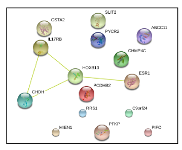
Figure 7.1: The STRING compact network view.

Rule	Antecedent	Conclusion	Support	Confidence
0	ESR1 $\uparrow$	GSTA2 $\uparrow$	1	100$\%$
1	RRS1 $\downarrow$ and ABCC11 $\uparrow$	CRISPLD2 $\uparrow$ and CHDH $\uparrow$	24	96$\%$
2	RRS1 $\downarrow$ and HOXB13 $\downarrow$	CRISPLD2 $\uparrow$	18	94$\%$
3	BLOC1S6 $\downarrow$ and HOXB13 $\downarrow$	CRISPLD2 $\uparrow$ and CHDH $\uparrow$	24	92$\%$
4	HOXB13 $\downarrow$ and ABCC11 $\uparrow$	BLOC1S6 $\downarrow$ and CHDH $\uparrow$	17	77$\%$
5	INSIG1 $\downarrow$	CRISPLD2 $\uparrow$, IRAK3 $\uparrow$ and ABCC11 $\uparrow$	19	70$\%$
6	IL17BR $\uparrow$	PFKP $\downarrow$	9	52$\%$
7	HOXB13 $\uparrow$	NDUFAF2 $\downarrow$	1	50$\%$
8	IL17BR $\uparrow$	C9orf24 $\uparrow$	8	47$\%$

Table 7.10: Association rules: Expression levels $\Rightarrow$ Expression levels.

According to Table 7.10, Rule 0 reflects that the estrogen receptor 1 which is a Nuclear hormone receptor and is expressed by ESR1 when it is over-expressed in this experiment induces an over-expression of the glutathione S-transferase alpha 2 traduced by gene GSTA2. Rule 3 highlights that if the HOXB13 and the BLOC1S6 genes are down-expressed then the CHDH and the CRISPLD2 genes are over-expressed. In fact, the HOXB13 gene refers to Sequence-specific transcription factor which is part of a developmental regulatory system that provides cells with specific positional identities on the anterior-posterior axis. While, the CRISPLD2 gene is cysteine-rich secretory protein LCCL domain and the CHDH gene expresses the choline dehydrogenase. Rule 6 present an interesting relation between the IL17BR gene, reflecting the interleukin 17 receptor B and playing a role in controlling the growth and differentiation of hematopoietic cells, and the PFKP gene corresponding to phospho-fructokinase, platelet. The PFKP gene catalyzes the phosphorylation of fructose-6-phosphate (F6P) by ATP to generate fructose-1, 6-bisphosphate (FBP) and ADP.

Almost of the obtained association rules highlights important relationship of the HOXB13 and the IL17BR genes. In fact, the analysis of these two genes expression may be useful for identifying patients appropriate for alternative therapeutic regimens in early-stage breast cancer [Ma et al., 2004]. In summary, we conclude that the diverse obtained rare correlated association-rules reveals a variety of relationship between up and down gene-expression which proves that breast cancer is an interesting biologically heterogeneous research field. Thus to deduce that rare correlated patterns present good results when applied to the context of biological data since they are able to reveal hidden and surprising relations among genes properties.

7.7 Conclusion

This chapter was dedicated to the description of the associative classification process based on the correlated patterns. For this purpose, we started by presenting the framework of association rules extraction, we clarify the properties of the generic bases of association rules. We continued with the detailed description and presentation of the application of both frequent correlated and rare correlated patterns within the classification of some UCI benchmark datasets. We equally present the application of rare correlated patterns in the classification of intrusion detection data from the KDD 99 dataset. The effectiveness of the proposed classification method has been experimentally proved. The chapter was concluded with the application of the $\mathcal{RCPR}$ representation on the extraction of biologically relevant associations among Micro-array gene expression data. A better classification accuracy may be achieved while thinking about missing-values treatment [Ben Othman and Ben Yahia, 2006].

Part IV Conclusion

Chapter 8 Conclusion and Perspectives

8.1 Conclusion

In this thesis, we were mainly interested to two complementary classes of patterns namely rare correlated patterns and frequent correlated patterns according to the bond correlation measure. In fact, the $\mathcal{FCP}$ set of frequent correlated patterns result from the intersection of the set of frequent patterns and the set of correlated patterns. The $\mathcal{FCP}$ set is then the result of the conjunction of two anti-monotonic constraints of frequency and of correlation. Consequently this $\mathcal{FCP}$ set induces an order ideal on the itemset lattice. Nevertheless, the $\mathcal{RCP}$ set of rare correlated patterns result from the conjunction of two constraints of distinct types namely the monotonic constraint of rarity and the anti-monotonic constraint of correlation. Thus, the localization of the $\mathcal{RCP}$ set is more difficult and the extraction process is more costly. This characteristic constitute one of the challenges to deal with through this thesis.

This thesis report was partitioned into four different parts. The first part was dedicated to the review of correlated patterns mining. In this regard, we started the first chapter of this part by introducing the basic notions related to the itemset search space, to itemset extraction. We defined the two distinct categories of constraints. We introduced equally the environment of Formal Concept Analysis FCA which offer the basis for the proposition of our approaches, specifically the notions of Closure Operator, Minimal Generator, Closed Pattern, Equivalence class and Condensed representation of a set of patterns. Thereafter, we studied in the second chapter of this first part, the state of the art approaches dealing with correlated patterns mining. Our study covers the frequent correlated patterns mining, the rare correlated patterns as well as the approaches focusing on condensed representations of correlated itemsets.

The second part was dedicated to the presentation of our approaches. The first chapter of this part was devoted to the characterization of both frequent correlated and rare correlated patterns and the introduction of their associated condensed representations. We deeply defined the properties of the $f_{bond}$ closure operator associated to the bond measure and we describe the structural specificities of the induces equivalence classes. In fact, the condensed representations associated to the $\mathcal{RCP}$ set of rare correlated are composed by the union of the closed correlated rare patterns and their associated minimal generators. Nevertheless, for the case of frequent correlated patterns, the closed correlated frequent patterns constitute a condensed concise representation of the $\mathcal{FCP}$ set. In the second chapter, we focused on the presentation of our Gmjp extraction approach. In fact, Gmjp is the first approach to mine bond correlated patterns in a generic way (i.e., with two types of constraints: anti-monotonic constraint of frequency and monotonic constraint of rarity). Our mining approach was based on the key notion of bitsets codification that supports efficient correlated patterns computation thanks to an adequate condensed representation of patterns. The deeply description of the whole steps of Gmjp as well as the theoretical complexity approximation and a running example were equally detailed. This fifth chapter was concluded by the algorithms of interrogation and of regeneration of the condensed representation associated to rare correlated patterns.

The third part of this report was dedicated to the experimental validation of our Gmjp as well as the presentation and evaluation of the associative-classification process. In the first chapter of this third part we focused on the experimental evaluation of Gmjp. The evaluation process was based on two main axes, the first is related to the compactness rates of the condensed representations while the second axe concerns the running time. We equally proposed an optimized version of Gmjp which present much better performance than Gmjp over different benchmark datasets. The two main keys which constitute the thrust of the improved version: (i) only one scan of the database is performed to build the new transformed dataset; (ii) it offers a resolution of the problem of handling both monotonic and anti-monotonic constraints within a unique mining process. In fact, opposite constraint mining is classified as an NP-Hard problem [Boley and Gärtner, 2009]. But, our goal was optimally achieved without relying on the border’s extraction. This constitute a strong added-value to Gmjp, since many approaches are based on border’s identification in order to extract such difficult set of patterns.

In the second chapter of this third part, we presented the classification process based on correlated patterns. Since the classification process that we proposed was based on associative rules, thus we started the chapter by presenting the framework of association rules extraction, we clarified the properties of the generic bases of association rules. We continued with the detailed presentation of the application of both frequent correlated and rare correlated patterns within the classification of some UCI benchmark datasets. In addition, we reported in this chapter the application of rare correlated patterns in the classification of intrusion detection data from the KDD 99 dataset. The obtained results showed the usefulness of our proposed classification method over four different intrusion classes. We concluded the chapter with the application of rare correlated associative rules on Micro-array gene expression data. The obtained rules helped to identify potential relations among up and down regulated gene expressions related to Breast Cancer.

The fourth and final part concluded the thesis report.

8.2 Perspectives

The obtained results in this thesis opens many perspectives from which we quote:

✓The extraction of generalized association rules starting from rare correlated patterns also from frequent correlated patterns. In addition, we plan to extend our approach to other correlation measures [Kim et al., 2011, Segond and Borgelt, 2011, Surana et al., 2010, Omiecinski, 2003] through classifying them into classes of measures sharing the same properties. An important direction is to propose a generic way allowing the extraction of the sets of frequent correlated patterns and rare correlated patterns as well as their associated concise representations. Pieces of new knowledge in the form of exact or approximate correlated generalized association rules can then be derived.

✓The extension of the extraction of correlated patterns to the extraction of both frequent and rare sequential correlated patterns. A promoting area for applying sequential patterns is: opinion mining. In fact, Opinion Mining is an important research area [Ohana et al., 2011] which is based on the extraction of opinions and the sentiment analysis from text data (Text Mining). Opinion Mining is a fruitful field since it is concerned with many real life application fields such as: Financial analysis, market estimation, customer behavior detection. In fact, the evaluation of new products and services nearby customers is based on the comments and advices of web visitors. Consequently, the derivation of association rules and their application to opinion mining [Jindal et al., 2010] is a potentially interesting research axe.

✓Another Fruitful perspective consists in addressing the issue of correlated patterns mining from big datasets. In fact, big data mining is a new challenging task since computational requirements are difficult to provide. An interesting solution is to exploit parallel frameworks, such as MapReduce [Wang et al., 2012] that offer the opportunity to make powerful computing and storage. Consequently, mining condensed representations of correlated patterns from big real life datasets thank to the MapReduce environment is an up to date challenging mining task.

8.3 Publication List

$\bullet$ Journals

[1] Bouasker Souad, Hamrouni Tarek, Ben Yahia Sadok. Motifs Corrélés rares: Caractérisation et nouvelles représentations concises exactes . Appeared in the Revue of New Information Technologies RNTI: Quality of Data and Knowledge: Measure and Evaluate the Quality of Data and Knowledge, (MQDC 2012), pages 89-116.[indexed DBLP].

 

[2] Bouasker Souad, Hamrouni Tarek, Ben Yahia Sadok. Efficient Mining of New Concise representations of Rare Correlated Patterns. Appeared in the IDA journal ’Intelligent Data Analysis’ 2015, Volume 19, pages 359-390. (Impact factor in 2014 = 0.50).

$\bullet$ International Conferences

[3] Bouasker Souad, Hamrouni Tarek, Ben Yahia Sadok. Algorithmes d’extraction et d’interrogation d’une représentation concise exacte des motifs corrélés rares. In proceedings of the 12th international francophone conference on extraction and managing knowledges (EGC 2012), Bordeaux, France, pages 225-230. [indexed DBLP], rank C.

 

[4] Bouasker Souad, Hamrouni Tarek, Ben Yahia Sadok. New Exact Concise Representation of Rare Correlated Patterns: Application to Intrusion Detection. In proceedings of the 16th Pacific Asia conference (PAKDD 2012), Kuala Lumpur, Malaysia, pages 61-72. [indexed IEEE, DBLP], rank A.

 

[5] Bouasker Souad, Ben Yahia Sadok. Inferring New Knowledge from Concise Representations of both Frequent and Rare Jaccard Itemsets. In proceedings of the 24th International conference of Database and Expert Systems Applications (DEXA 2013), Prague, Check Republic, pages 109-123. [indexed IEEE, DBLP], rank B.

 

[6] Bouasker Souad, Ben Yahia Sadok. Key Correlation Mining by Simultaneous Monotone and Anti-monotone Constraints Checking. In proceedings of the 30th ACM Symposium on Applied Computing (SAC 2015), Salamanca, Spain. [indexed ACM, IEEE, DBLP], rank B.

Bibliography

- [Agrawal and Srikant, 1994] Agrawal, R. and Srikant, R. (1994). Fast algorithms for mining association rules in large databases. In Proceedings of the 20th International Conference on Very Large Data Bases (VLDB 1994), Santiago, Chile, pages 487–499.
- [Alagukumar and Lawrance, 2015] Alagukumar, S. and Lawrance, R. (2015). Algorithm for microarray cancer data analysis using frequent pattern mining and gene intervals. In National Conference on Research Issues in Image Analysis and Mining Intelligence (NCRIIAMI-2015), pages 9–14.
- [Ayouni et al., 2010] Ayouni, S., Laurent, A., Ben Yahia, S., and Poncelet, P. (2010). Mining closed gradual patterns. In Artificial Intelligence and Soft Computing, 10th International Conference, ICAISC 2010, Zakopane, Poland, June 13-17, 2010, Part I, pages 267–274.
- [Barsky et al., 2012] Barsky, M., Kim, S., Weninger, T., and Han, J. (2012). Mining flipping correlations from large datasets with taxonomies. In Proceedings of the 38th International Conference on Very Large Databases - VLDB 2012, Istanbul, Turkey, pages 370–381.
- [Bastide et al., 2000] Bastide, Y., Taouil, R., Pasquier, N., Stumme, G., and Lakhal, L. (2000). Mining frequent patterns with counting inference. ACM-SIGKDD Explorations, 2(2):66–75.
- [Ben Amor et al., 2004] Ben Amor, N., Benferhat, S., and Elouedi, Z. (2004). Naive bayes vs decision trees in intrusion detection systems. In Proceedings of the ACM Symposium on Applied Computing (SAC 2004), Nicosia, Cyprus, 2004, pages 420–424.
- [Ben Othman and Ben Yahia, 2006] Ben Othman, L. and Ben Yahia, S. (2006). Yet another approach for completing missing values. In Concept Lattices and Their Applications, Fourth International Conference, CLA 2006, Tunis, Tunisia, October 30 - November 1, 2006, Selected Papers, pages 155–169.
- [Ben Younes et al., 2010] Ben Younes, N., Hamrouni, T., and Ben Yahia, S. (2010). Bridging conjunctive and disjunctive search spaces for mining a new concise and exact representation of correlated patterns. In Proceedings of the 13th International Conference Discovery Science (DS 2010), LNCS, volume 6332, Springer-Verlag, Canberra, Australia, pages 189–204.
- [Boley and Gärtner, 2009] Boley, M. and Gärtner, T. (2009). On the complexity of constraint-based theory extraction. In Proceedings of the 12th International Conference Discovery Science (DS 2009), LNCS, volume 5808, Springer-Verlag, Porto, Portugal, pages 92–106.
- [Bonchi et al., 2005] Bonchi, F., Giannotti, F., Mazzanti, A., and Pedreschi, D. (2005). Efficient breadth-first mining of frequent pattern with monotone constraints. Knowledge and Information Systems, 8(2):131–153.
- [Bonchi and Lucchese, 2006] Bonchi, F. and Lucchese, C. (2006). On condensed representations of constrained frequent patterns. Knowledge and Information Systems, 9(2):180–201.
- [Bouasker and Ben Yahia, 2013] Bouasker, S. and Ben Yahia, S. (2013). Inferring knowledge from concise representations of both frequent and rare jaccard itemsets. In Proceedings of the 24th International Conference on Databases and Expert Systems Applications (DEXA 2013), Prague, Czech Republic.
- [Bouasker and Ben Yahia, 2015] Bouasker, S. and Ben Yahia, S. (2015). Key correlation mining by simultaneous monotone and anti-monotone constraints checking. In Proceedings of The 30th ACM/SIGAPP Symposium On Applied Computing, SAC 2015, Salamanca, Spain, pages 851–856.
- [Bouasker et al., 2012a] Bouasker, S., Hamrouni, T., and Ben Yahia, S. (2012a). Algorithmes d’extraction et d’interrogation d’une représentation concise exacte des motifs corrélés rares : Application à la détection d’intrusions. In Extraction et gestion des connaissances (EGC’2012), Actes, janvier 31 - février 2012, Bordeaux, France, pages 225–230.
- [Bouasker et al., 2012b] Bouasker, S., Hamrouni, T., and Ben Yahia, S. (2012b). Motifs corrélés rares: caractérisation et nouvelles représentations concises. In Revue des Nouvelles Technologies d’Information, RNTI 2012), pages 89–106.
- [Bouasker et al., 2012c] Bouasker, S., Hamrouni, T., and Ben Yahia, S. (2012c). New exact concise representation of rare correlated patterns: Application to intrusion detection. In Proceedings of the 16th Pacific-Asia Conference on Knowledge Discovery and Data Mining (PAKDD 2012), Kuala Lumpur, Malaysia, pages 61–72.
- [Bouasker et al., 2015] Bouasker, S., Hamrouni, T., and Ben Yahia, S. (2015). Efficient mining of new concise representations of rare correlated patterns. Intelligent Data Analysis, 19(2):359–390.
- [Bouker et al., 2014] Bouker, S., Saidi, R., Ben Yahia, S., and Nguifo, E. M. (2014). Mining undominated association rules through interestingness measures. International Journal on Artificial Intelligence Tools, 23(4).
- [Boulicaut and Jeudy, 2010] Boulicaut, J.-F. and Jeudy, B. (2010). Constraint-based data mining. In Data Mining and Knowledge Discovery Handbook (2nd edition), Springer, pages 339–354.
- [Brahmi et al., 2011] Brahmi, I., Ben Yahia, S., Aouadi, H., and Poncelet, P. (2011). Towards a multiagent-based distributed intrusion detection system using data mining approaches. In Agents and Data Mining Interaction - 7th International Workshop on Agents and Data Mining Interation, ADMI 2011, Taipei, Taiwan, May 2-6, 2011, Revised Selected Papers, pages 173–194.
- [Brahmi et al., 2010] Brahmi, I., Ben Yahia, S., and Poncelet, P. (2010). MAD-IDS: novel intrusion detection system using mobile agents and data mining approaches. In Intelligence and Security Informatics, Pacific Asia Workshop, PAISI 2010, Hyderabad, India, June 21, 2010. Proceedings, pages 73–76.
- [Brin et al., 1997] Brin, S., Motwani, R., and Silverstein, C. (1997). Beyond market baskets: generalizing association rules to correlations. In Proceedings of the ACM-SIGMOD International Conference on Management of Data (SIGMOD 1997), Washington D. C., USA, pages 265–276.
- [Bucila et al., 2003] Bucila, C., Gehrke, J., Kifer, D., and White, W. M. (2003). DualMiner: A dual-pruning algorithm for itemsets with constraints. Data Mining knowledge Discovery, 7(3):241–272.
- [Cohen et al., 2000] Cohen, E., Datar, M., Fujiwara, S., Gionis, A., Indyk, P., R.Motwani, D.Ullman, J., and Yang, C. (2000). Finding interesting associations without support pruning. In Proceedings of the 16th International Conference on Data Engineering (ICDE 2000), IEEE Computer Society Press, San Diego, California, USA, pages 489–499.
- [Davey and Priestley, 2002] Davey, B. and Priestley, H. (2002). Introduction to Lattices and Order. Cambridge University Press.
- [De Raedt et al., 2002] De Raedt, L., Jaeger, M., Lee, S. D., and Mannila, H. (2002). A theory of inductive query answering. In Proceedings of the 2nd International Conference on Data Mining (ICDM 2002), IEEE Computer Society Press, Maebashi City, Japan, pages 123–130.
- [El-Hajj et al., 2005] El-Hajj, M., Zaïane, O. R., and Nalos, P. (2005). Bifold constraint-based mining by simultaneous monotone and anti-monotone checking. In Proceedings of the 5th International Conference on Data Mining (ICDM 2005), IEEE Computer Society Press, Houston, Texas, USA, pages 146–153.
- [Farid et al., 2010] Farid, M., Harbi, N., Bahri, E., Rahman, M., and Rahman, C. (2010). Attacks classification in adaptive intrusion detection using decision tree. In Proceedings of the International Conference on Computer Science (ICCS’10), Rio De Janeiro, Brazil.
- [Galambos and Simonelli, 2000] Galambos, J. and Simonelli, I. (2000). Bonferroni-type inequalities with applications. Springer.
- [Ganter and Wille, 1999] Ganter, B. and Wille, R. (1999). Formal Concept Analysis. Springer.
- [Gasmi et al., 2007] Gasmi, G., Ben Yahia, S., Nguifo, E. M., and Bouker, S. (2007). Extraction of association rules based on literalsets. In Data Warehousing and Knowledge Discovery, 9th International Conference, DaWaK 2007, Regensburg, Germany, September 3-7, 2007, Proceedings, pages 293–302.
- [Gasmi et al., 2005] Gasmi, G., Ben Yahia, S., Nguifo, E. M., and Slimani, Y. (2005). IGB: A new informative generic base of association rules. In Advances in Knowledge Discovery and Data Mining, 9th Pacific-Asia Conference, PAKDD 2005, Hanoi, Vietnam, May 18-20, 2005, pages 81–90.
- [Grahne et al., 2000] Grahne, G., Lakshmanan, L. V. S., and Wang, X. (2000). Efficient mining of constrained correlated sets. In Proceedings of the 16th International Conference on Data Engineering (ICDE 2000), IEEE Computer Society Press, San Diego, California, USA, pages 512–521.
- [Guns, 2016] Guns, T. (2016). Towards generic and efficient constraint-based mining, a constraint programming approach. In 16éme Journées Francophones Extraction et Gestion des Connaissances, EGC 2016, 18-22 Janvier 2016, Reims, France, pages 13–20.
- [Guns et al., 2013] Guns, T., Dries, A., Tack, G., Nijssen, S., and Raedt, L. D. (2013). Miningzinc: A modeling language for constraint-based mining. In The 23rd International Conference on Artificial Intelligence, ICAI 2013, Beijing, China.
- [Hamrouni et al., 2008] Hamrouni, T., Ben Yahia, S., and Mephu Nguifo, E. (2008). Generic Association Rule Bases: Are They so Succinct? Selected Papers of the 4th International Conference Concept Lattices and Their Applications (CLA 2006), LNCS, volume 4923, Springer-Verlag, Hammamet, Tunisia. pages 198–213.
- [Hamrouni et al., 2015] Hamrouni, T., Slimani, S., and Ben Charrada, F. (2015). A data mining correlated patterns-based periodic decentralized replication strategy for data grids. Journal of Systems and Software, 110:10 –27.
- [Hu and Li, 2009] Hu, J. and Li, X. (2009). Association rules mining including weak-support modes using novel measures. WSEAS Transactions on Computer, 8:559–568.
- [Jaccard, 1901] Jaccard, P. (1901). Étude comparative de la distribution orale dans une portion des Alpes et des Jura. Bulletin de la Société Vaudoise des Sciences Naturelles, 37:547–579.
- [Jindal et al., 2010] Jindal, N., Liu, B., and Lim, E. (2010). Finding unusual review patterns using unexpected rules. In In Proceedings of the international Conference on Information and Knowledge Management (CIKM’10), Toronto, Ontario, Canada, pages 1549–1552.
- [Karim et al., 2012] Karim, M., Halder, S., Jeong, B., and Choi, H. (2012). Efficient Mining Frequently Correlated, Associated-Correlated and Independent Patterns Synchronously by Removing Null Transactions, volume 182, chapter Lecture Notes in Electrical Engineering, pages 93–103.
- [Kim et al., 2011] Kim, S., Barsky, M., and Han, J. (2011). Efficient mining of top correlated patterns based on null-invariant measures. In Proceedings of the 15th European Conference on Machine Learning and Knowledge Discovery in Databases (ECML-PKDD 2011), LNCS, volume 6912, Springer, Athens, Greece, pages 177–192.
- [Kim et al., 2004] Kim, W. Y., Lee, Y. K., and Han, J. (2004). Ccmine: efficient mining of confidence-closed correlated patterns. In Proceedings of the 8th International Pacific-Asia Conference on Knowledge Data Discovery (PAKDD 2004), Sydney, Australie, pages 569–579.
- [Kiran and Kitsuregawa, 2013] Kiran, R. U. and Kitsuregawa, M. (2013). Mining correlated patterns with multiple minimum all-confidence thresholds. In Proceedings of the 17th Pacific-Asia Conference on Knowledge Discovery and Data Mining (PAKDD 2013), pages 295–306.
- [Koh and Rountree, 2010] Koh, Y. S. and Rountree, N. (2010). Rare Association Rule Mining and Knowledge Discovery: Technologies for Infrequent and Critical Event Detection. IGI Global Publisher.
- [Kryszkiewicz, 2002] Kryszkiewicz, M. (2002). Concise representation of frequent patterns and association rules. Habilitation dissertation, Institute of Computer Science, Warsaw University of Technology, Warsaw, Poland.
- [Le Bras et al., 2011] Le Bras, Y., Lenca, P., and Lallich, S. (2011). Mining classification rules without support: an anti-monotone property of jaccard measure. In Proceedings of the 14th international conference on Discovery science - DS 2011, Espoo, Finland, pages 179–193.
- [Lee et al., 2006a] Lee, A. J. T., Lin, W. C., and Wang, C.-S. (2006a). Mining association rules with multi-dimensional constraints. The Journal of Systems and Software, 79(1):79–92.
- [Lee et al., 2006b] Lee, A. J. T., Lin, W. C., and Wang, C.-S. (2006b). Mining association rules with multi-dimentional constraints. The Journal of Systems and Software, 79(1):79–92.
- [Lee and De Raedt, 2004] Lee, S. D. and De Raedt, L. (2004). An efficient algorithm for mining string databases under constraints. In Proceedings of the 3rd International Workshop on Knowledge Discovery in Inductive Databases (KDID 2004), LNCS, volume 3377, Springer-Verlag, Pisa, Italy, pages 108–129.
- [Lee et al., 2003] Lee, Y. K., Kim, W. Y., Cai, Y. D., and Han, J. (2003). CoMine: efficient mining of correlated patterns. In Proceedings of the 3rd International Conference on Data Mining (ICDM 2003), IEEE Computer Society Press, Melbourne, Florida, USA, pages 581–584.