Taming Polar Active Matter with Moving Substrates: Directed Transport and Counterpropagating Macrobands

Abstract

Following the goal of using active particles as targeted cargo carriers aimed, for example, to deliver drugs towards cancer cells, the quest for the control of individual active particles with external fields is among the most explored topics in active matter. Here, we provide a scheme allowing to control collective behaviour in active matter, focusing on the fluctuating band patterns naturally occurring e.g. in the Vicsek model. We show that exposing these patterns to a travelling wave potential tames them, yet in a remarkably nontrivial way: the bands, which initially pin to the potential and comove with it, upon subsequent collisions, self-organize into a macroband, featuring a predictable transport against the direction of motion of the travelling potential. Our results provide a route to simultaneously control transport and structure, i.e. micro- versus macrophase separation, in polar active matter.

I Introduction

Active matter contains self-propelled particles like bacteria, algae, or synthetic autophoretic Janus colloids whose properties can be designed on demand Ramaswamy2010 ; Marchetti2013 ; Bechinger2016 . As one of their main characteristics, these systems are intrinsically out of equilibrium allowing them to self-organize into new ordered and even functional structures. In synthetic active systems, such structures include dynamic clusters which dynamically form and break-up in low density Janus colloids Theurkauff2012 ; Palacci2013 ; Buttinoni2013 ; Ginot2018 ; Liebchen2018 as well as laser driven colloids which spontaneously start to move ballistically (self-propel) when binding together Soto2014 ; Varma2018 ; Schmidt2018 . Likewise, biological microswimmers form patterns such as vortices in bacterial turbulence Sokolov2012 ; Wensink2012 ; Kaiser2014 ; Stenhammar2017 , or swirls and microflock patterns in chiral active matter like curved polymers or sperm Riedel2005 ; Loose2014 ; Denk2016 ; LiebchenLevis2017 .

Much of what we know about active systems and the patterns they form roots in explorations of minimal models which to some extend represent broader classes of active systems showing the same symmetries. The pioneering example of such a minimal model is the Vicsek model describing polar self-propelled particles such as actin-fibres mixed with motor proteins Schaller2010 ; Goff2016 , certain microorganisms Toner2005 , self-propelled rods Paxton2004 ; Peruani2016 or “birds” Toner1995 ; Toner2005 which only see their neighbors and have a tendency to align with them, in competition with noise. While forbidden in equilibrium Mermin1966 the Vicsek model shows true long-range order in two dimensions Toner1995 , meaning that activity makes orientational correlations robust against noise over arbitrarily long distances. The phase transition from the disordered phase which occurs for strong noise to the long-range ordered Toner-Tu phase is now known to be discontinuous Chate2004 and features a remarkably large coexistence region Caussin2014 ; Solon2015 where high-density bands of comoving polarized particles spontaneously emerge and traverse through a background of a low-density disordered gas-like phase. These bands behave highly randomly; they merge when colliding with each other but also split up frequently, rendering an irregular pattern of sharply localized and strongly polarized moving bands. The latter choose their direction of motion spontaneously depending on initial state and fluctuating molecular environment (noise realization); thus, when averaging over many realizations, there is no net motion. This randomness is unfortunate in view of potential key applications of active matter, e.g. for targeted drug delivery, crucially requiring schemes to control active particles. Here, while single particle guidance with external fields is among the most explored problems in active matter Palacci2013 ; Koumakis2013 ; Ma2015 ; Ebbens2016 ; Geiseler2016 ; Demirors2017 ; Colabrese2017 ; Geiseler2017 ; Muinos2018 and there is a moderate knowledge on interacting particles in external fields (complex environments) Drocco2012 ; Ginot2015 ; Kuhr2017 ; Reichhardt2017a ; Zhu2018 ; Reichhardt2018b and their control Yan2016 ; Peng2016 ; Guillamat2016 ; Guillamat2017 ; Kaiser2017 , surprisingly little is known about the controllability of polar active particles and band patterns they naturally form.

In the present work we ask for a scheme to tame band patterns, i.e. if we can force the bands in the Vicsek model to settle down into a pattern featuring a predictable and externally controllable direction of motion. To achieve this, we apply a “traveling wave potential” (also called travelling potential ratchet Reimann2002 ) to the Vicsek model. We find that such an external field does in fact allow to control the late time direction of motion of particle ensembles in polar active matter, yet, in a remarkably nontrivial way. In our simulations, for appropriate parameter regimes, we see the formation of bands that at early times pin to the minima of the travelling potential and comove with it. When time proceeds, one of the bands suddenly unpins and starts counterpropagating in the travelling potential. Upon subsequent collisions the band swells towards a macroband containing most particles in the system. This macroband emerges representatively in a large parameter window and shows a predictable motion against the travelling direction of the potential. Our results show that a moving (or tilted, see Fig. 1) substrate tames the collective behaviour of polar active particles and can be used to control the transition from microphase separation (band patterns) to a macrophase separated state which does show predictable transport. In the following, we specify these results and analyze the mechanism underlying the emergence of a counterpropagating macroband.

II Model

We consider $N=5000$ active overdamped particles in a quasi-1D-potential $V(x,y,t)$, which is uniform in $y$-direction and represents a traveling wave in $x$-direction; i.e. it is periodically modulated and moves with constant speed $v_{L}=\omega/k$ in $x$-direction, where $\omega,k$ are the frequency and wave vector of the travelling potential (Fig. 1 (b)). Such a potential has previously been considered for active point particles Zhu2018 and disks Sandor2017 and can be realized e.g. by a micropatterned ferrite garnet film substrate Tierno2016 , by optical lattices traversing at speeds of a few $\mu/s$, or effectively (see Fig.  1 (c)), simply by a tilted washboard potential Hanggi2009 ; Juniper2016 ; Juniper2017 . Note here that in the comoving frame (moving with a constant velocity $v_{L}$) the dynamics translates into motion of a particle in a static tilted washboard potential (see Fig. 1 (b),(c) and Sec. IV).
Besides experiencing the external potential, the active particles also self-propel, a fact effectively described by a self-propulsion force $\gamma v_{0}{\bf p}_{i}$ where $\mathbf{p}_{i}=\cos\theta_{i}\mathbf{e}_{x}+\sin\theta_{i}\mathbf{e}_{y};\;i=1,..,N$ are the self-propulsion directions of the particles and $\gamma$ is the Stokes drag coefficient. In bulk, the particles would move with a constant speed $v_{0}$. As in the Vicsek model, we assume that the particles align with each other. We define the dynamics of the particles by the following equations of motion footnote2 :

$$\dot{\bf r}_{i} = v_{0}{\bf p}_{i}+{\bf F}_{i}/\gamma$$ (1a)

$$\dot{\theta}_{i} = \frac{g}{\pi R^{2}}\sum_{j\in\delta_{i}}^{N}\sin\left(\theta_{j}-\theta_{i}\right)+\sqrt{2D_{r}}\eta_{i}(t)$$ (1b)

Here, $g$ controls the strength of alignment of a particle with its neighbors within a range $R$ and the sum is performed over all these neighbors (see Fig. 1 (a)). Alignment competes with rotational Brownian diffusion, occurring with a rate $D_{r}$; $\eta_{i}$ represents Gaussian white noise of zero mean and unit variance. The force due to the substrate reads

$${\bf F}_{i}:=-\nabla U=\gamma u_{0}\cos\left(2\pi\left(kx_{i}-\omega t\right)\right){\bf e}_{x}$$ (2)

where $u_{0}$ is the strength of the external force. Here, in all of our results we express lengths and times in units of $\mu m$ and $s$ respectively, i.e. we introduce parameters $D_{r}^{\prime}=D_{r}\cdot s,~{}g^{\prime}=g\cdot s/\mu m^{2}$ etc. and omit primes for simplicity, allowing thus for a straightforward comparison with potential experiments. However, for readers interested in the actual dimensionless control parameters, see footnote1 .

We now study the dynamics of the described model using Brownian dynamics simulations and an elongated simulation box of size $L_{x}\times L_{y}=500\times 5$, fixing the density to $\rho=2$, as well as random but uniformly distributed initial particle positions and orientations. Using more quadratic boxes leads to qualitatively similar phenomena.

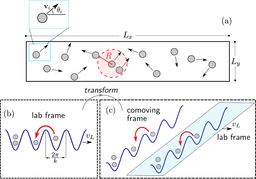
Figure 1: (a) Cartoon of the polar active particles (a) in a traveling wave potential (b), with a velocity $v_{L}=\omega/k$. Here $\mathbf{v}_{i}=v_{0}\mathbf{p}_{i}$ is the self-propulsion velocity of the $i$-th particle, aligning with adjacent partices (red circle). A Galilei transformation to the comoving frame turns the travelling wave potential (panel (b)) into a static, tilted periodic potential (panel (c)). Thus, motion in the travelling wave potential (b) is equivalent to motion in a static tilted lattice in the comoving frame which displaces through space (relative to the laboratory frame) with a constant speed $v_{L}$ (panel (c)). The pinned state, where particles comove with the travelling wave corresponds to particles resting around a minimum of the tilted lattice in (c). We find that in the lab frame, for certain values of the parameters, polar active particles can move faster down the tilted lattice (to the left) than the lattice displaces through space (see Sec IV). The dynamical pathway to achieve this sliding state involves a controllable transition from microphase separation (patterns) to macrophase separation (counterpropagating macroband).

III Counterpropagating Macroband

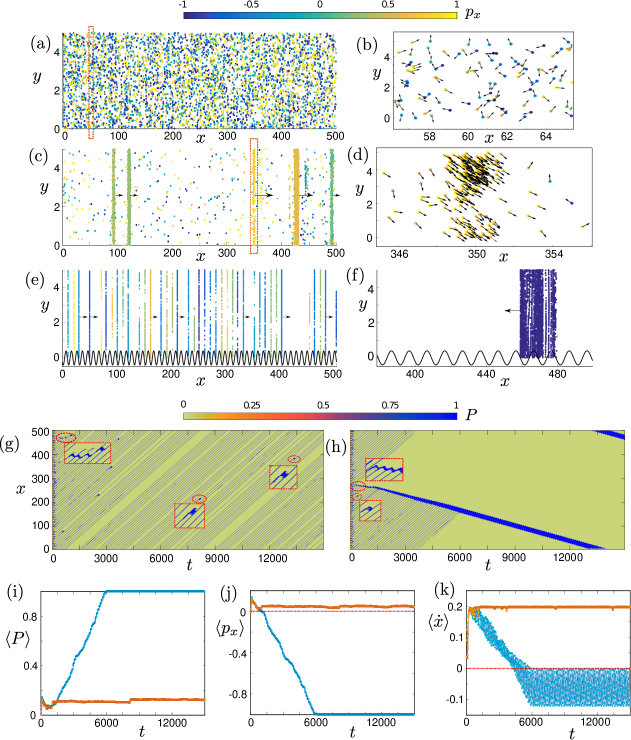
Figure 2: (a),(b),(c),(d) Snapshots of (a) the disordered uniform phase and (c) the bands formed in the ordered phase in the absence of the lattice from sample simulations at $D_{r}=0.151$ and $D_{r}=0.003$ respectively. The corresponding zoomed-in figures (b),(d) demonstrate the direction of the particles’ motion. (e),(f) Snapshots of the two different ordered phases: (e) pinned phase and (f) sliding phase in the presence of a lattice from sample simulations at $D_{r}=0.0003$. Note that the shown ’sine wave’ illustrates the lattice focusing on its wavelength. In all the above cases (a)-(f) the colors denote the polarization of each particle along the $x$ direction $p_{x,i}=\cos\theta_{i}$.(g),(h) The polarization $P_{n}$ of the formed bands (Eq. (3)), depicted by color, as a function of the time and the $x$ coordinate for sample simulations of (g) the pinned phase and (h) the sliding phase at $D_{r}=0.0003$. The insets provide zooms of some special events during dynamics featuring band collisions. (i)-(k) Time evolution of (i) the average polarization $\left<P\right>$, (j) the average cosine of the particles $\left<p_{x}\right>=\left<\cos\theta_{i}\right>$ and (k) the average particle velocity $\left<\dot{x}\right>$ for the pinned (dark orange line) and the sliding phase (blue line) of (g),(h). In the above cases the parameters of our setup read $g=0.07$, $D_{r}^{c}=0.15$, $N=5000$, $L_{x}=500$, $L_{y}=5$, $v_{0}=0.2$ and in most cases $u_{0}=0.3,\omega=0.02,k=0.1$ ($v_{L}=0.2$).

In the absence of a lattice, our simulations reveal the usual phenomenology of the Vicsek model Chate2004 ; Caussin2014 ; Solon2015 : For a given alignment strength ($g=0.07$) and comparatively strong noise $D_{r}>D_{r}^{c}\approx 0.15$ (or high temperatures), we find a disordered uniform phase (Fig. 2 (a),(b)), whereas noise values $D_{r}<D_{r}^{c}$ lead to a polarized phase (Fig. 2 (c),(d)). In the latter phase, particles self-organize into polarized bands of high density which move with a speed $\sim v_{0}$ and coexist with gas-like unpolarized regions in between the bands. The bands occur at seemingly irregular distances to each other. As time proceeds, they occasionally split up (for $D_{r}\neq 0$) and typically merge when they collide with each other; overall, the number and size of the bands changes dynamically.

In the presence of the traveling wave (moving lattice) and at weak noise ($D_{r}=3\times 10^{-4}<D_{r}^{c}$) the behaviour of the bands may change dramatically. While very steep lattices of course pin the particles permanently to the lattice minima, leading to a state where all particles comove with the lattice, shallow lattices have little impact on the behaviour of the system and its tendency to form bands. In this latter regime, the lattice exerts a periodic force which essentially averages out before the particles move much. Thus, we here focus on moderate lattice depth ($u_{0}=0.3$) and lattice speeds comparable to that of the particles ($v_{0}=v_{L}=0.2$), so that the particles can occasionally overcome the potential maxima. In this regime, for sufficiently weak noise (here $D_{r}<D_{r}^{c}=3\times 10^{-4}$), particles form quickly bands, most of which are pinned to the lattice and thus co-move with it (Fig. 2 (e),(g),(h)). Note that the polarization of such bands

$$P_{n}=\sqrt{\left(\sum_{i\in\textrm{band}~{}n}\cos\theta_{i}\right)^{2}+\left(\sum_{i\in\textrm{band}~{}n}\sin\theta_{i}\right)^{2}}$$ (3)

is almost unity even for small times and maintains this very high value during the time evolution (Fig. 2 (g),(h)). Occasionally, we observe that a band, assisted by the existing noise, changes direction and counterpropagates; it then soon collides with another band (see Fig. 2 (g),(h) insets for such collision events). Here, the two bands merge and form one larger band which in some cases becomes pinned and in other cases slides, still against the direction of motion of the lattice. In the latter case, the band soon encounters further bands and can in each case, either stop moving (get pinned to the lattice) or continue sliding. One might expect that this seemingly random result of the collision processes should ultimately lead back to a pinned state. Strikingly, however, in many simulations we observe cases where a band counterpropagates through the entire lattice and systematically consumes all other bands. The result is one macroband which contains most of the $N$ particles and counterpropagates against the direction of lattice motion (Fig. 2 (f),(h)). Since the particles counterpropagate, even when viewed from the laboratory frame, with respect to the forces acting on a pinned particle in a minimum of the lattice, they feature an absolute negative mobility. Thus, we observe a spontaneous reversal from a comoving state where most particles have followed the lattice to a counterpropagating state.

The striking difference between a finally pinned (Fig. 2 (e),(g)) and a finally sliding state (Fig. 2 (f),(h)) featuring a current reversal is further illustrated in Fig. 2 (i),(j),(k). Here we observe that the mean polarization (averaged over all particles) $\left<P\right>=\sqrt{\left<\cos\theta\right>^{2}+\left<\sin\theta\right>^{2}}$ increases from the pinned state at short times to a value of almost one for the sliding macroband (Fig. 2 (i)). It turns out (Fig. 2 (j)) that $\left<p_{x}\right>=\left<\cos\theta\right>\approx-1$, meaning that the particles collective self-propel against the direction of the lattice motion (still in the laboratory frame), i.e. along $-\mathbf{e}_{x}$. The average velocity of the particles is $\left<\dot{x}\right>\approx v_{L}=0.2$ (see also Eq. (1a)) for the pinned state (Fig. 2 (k)) and acquires a negative value oscillating in time for the case of the sliding macroband.

IV Pinned and sliding solutions

We can get some first insight into the mechanism underlying the surprising counterpropagation of the bands by examining the single-particle dynamics in the zero noise limit. When projected to the $x$-axis Eq. (1a) reduces to

$$\dot{\tilde{x}}={\tilde{v}_{x}}+\tilde{u}_{0}\cos\tilde{x},$$ (4)

where the Galilean transformation to the comoving frame $\tilde{x}=2\pi\left(kx-\omega t\right)$ is used, with  $\tilde{v}_{x}=2\pi k\left(v_{0}p_{x}-v_{L}\right)$, $-1\leq p_{x}=\cos\theta\leq 1$ and $\tilde{u}_{0}=2\pi ku_{0}$. This equation is well known as the overdamped limit of the equations of motion of e.g. the forced nonlinear pendulum Coullet2005 , the driven Frenkel-Kontorova (FK) model FKbook1 and the resistively shunted junction (RSJ) model of Josephson junctions Barone1982 . It is known to attain two different kinds of solutions depending on the value of $\frac{\tilde{v}_{x}}{\tilde{u}_{0}}$. For $\left|\frac{\tilde{v}_{x}}{\tilde{u}_{0}}\right|\leq 1$ the system is in the so-called pinned phase where the particle cannot overcome the potential barrier $\tilde{u}_{0}$ and remains therefore trapped within one of its wells ($\left<\tilde{x}\right>_{t}^{\infty}\rightarrow 0)$, yielding an asymptotic time averaged velocity $\left<\dot{x}\right>_{t}^{\infty}=v_{L}=\omega/k$. In the opposite case $\left|\frac{\tilde{v}_{x}}{\tilde{u}_{0}}\right|>1$, the particle is fast enough to overcome the potential barrier separating the wells (or in the example of the pendulum to lead to a rotation) and thus the system exhibits a sliding phase where the particle permanently moves (slides or rotates) in one and the same direction with an oscillating velocity $\dot{x}$ Cheng2015 of period $T=\frac{2\pi}{\sqrt{{\tilde{v}_{x}}^{2}-\tilde{u}_{0}^{2}}}$ Cheng2015 and an asymptotic time averaged velocity

$$\left<\dot{x}\right>_{t}^{\infty}=\textrm{sgn}\left(v_{0}p_{x}-v_{L}\right)\sqrt{\left(v_{0}p_{x}-v_{L}\right)^{2}-u_{0}^{2}}+v_{L}.$$ (5)

For the $N$-particle system (Eqs.(1a),(1b)) the particles’ self-propulsion directions $\mathbf{p}_{i}$ change due to alignment interactions (Eq. (1b)) and noise (Eq.(1a)). Hence, the projection of the particle speed onto the $x$-axis changes in time, so that the sliding condition $\left|\frac{\tilde{v}_{x}}{\tilde{u}_{0}}\right|>1$ subsequently may and may not be fulfilled. In terms of $\mathbf{p}_{i}$, the sliding condition reads

$$-1<{p_{x}}_{i}=\cos\theta_{i}<\frac{v_{L}-u_{0}}{v_{0}}~{}~{}\textrm{or}~{}~{}1>{p_{x}}_{i}>\frac{v_{L}+u_{0}}{v_{0}}.$$ (6)

In the present parameter regime ($v_{0}=v_{L}=0.2,~{}u_{0}=0.3$) sliding occurs for ${p_{x}}_{i}<-\frac{1}{2}$, or $\theta_{i}\in\left[\frac{2\pi}{3},\frac{4\pi}{3}\right].$ Thus roughly $1/3$ of particles will initially be in the sliding phase. Importantly, all of these particles which can in principle slide, move against the direction of lattice motion (negative ${p_{x}}_{i}$), i.e. sliding can only occur against the direction of lattice motion, as observed in Figs. 2 (f),(h),(j),(k). The main effect of rotational diffusion (noise in the particle orientations) consists in the smoothening of the pinned-to-sliding transition at $\left|\frac{\tilde{v}_{x}}{\tilde{u}_{0}}\right|=1$.

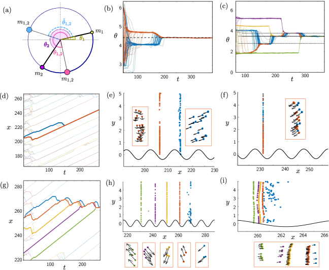
Figure 3: (a) Schematic illustration of the mechanism of merging for two bands with angles $\theta_{1}$ and $\theta_{2}$ and masses $m_{1}$, $m_{2}$ leading to the formation of a large band with angle $\theta_{1,2}$ (stable) or $\tilde{\theta}_{1,2}$ (unstable). (b) Time evolution of the angles $\theta$ of two colliding bands which after their merging become pinned in the lattice (see also subfigures (d)-(f)). (c) Time evolution of the angles $\theta$ of five bands colliding successively with each other, leading to the formation of a large sliding band (see also subfigures (g)-(i)). (d) Time evolution of the $x$ coordinate of two bands which after their merging become pinned in the lattice. Figures (e) and (f) provide corresponding snapshots before and after the collision, respectively. (g) Time evolution of the $x$ coordinate of five bands which successively collide and merge, initiating the formation of the large sliding band. Figures (h) and (i) provide corresponding snapshots before the first and after the final collision, respectively. In the above cases the parameters of our setup read $g=0.07$, $D_{r}^{c}=0.15$, $N=5000$, $L_{x}=500$,$L_{y}=5$, $v_{0}=0.2$,$D_{r}=3\times 10^{-4}$, $u_{0}=0.3,\omega=0.02,k=0.1$ ($v_{L}=0.2$).

V Collisions of Vicsek Bands

We now exploit these considerations regarding pinned and sliding states for single particles to understand the dynamics of the polarized bands in the lattice. In our simulations, shortly after their formation, the magnitude of the polarization of the individual bands quickly approaches a value close to one (Fig. 2 (g),(h)), i.e. most bands are moving with almost constant individual velocities relative to the lattice. Thus, in the absence of collisions, the bands essentially behave like single particles and are either pinned or slide through the lattice. To study band collisions, it is useful to assign effective “masses” $m_{n}$ to the bands representing the number of particles contained in the band. When two bands with polarization angles $\theta_{1},\theta_{2}$ and masses $m_{1},m_{2}$ collide, they usually merge into a larger band of total mass $m_{1,2}=m_{1}+m_{2}$ (Fig. 3(a)) and average their polarizations. (Formally, there are two fixpoints of the orientational dynamics when two bands merge: one reads $\theta_{1,2}=\Theta_{0}$ with $\Theta_{0}=\frac{m_{1}\theta_{1}+m_{2}\theta_{2}}{m_{1}+m_{2}}$, the other one $\theta_{1,2}=\Theta_{0}-2\pi\frac{m_{1}}{m_{1}+m_{2}}$; here the one lying within the smaller arc between $\theta_{1}$ and $\theta_{2}$ is stable and thus observed, the other one is unstable.)

In our simulations, the polarization direction of an isolated band can freely rotate (Goldstone mode); noise therefore creates a random dynamics of the band polarization direction. Once the polarization angle of an initially pinned band reaches a value $\theta_{1}\in(\frac{2\pi}{3},\frac{4\pi}{3}$) the band will move over a lattice barrier in the direction opposite to the lattice motion (Figs. 3(d),(e),(g),(h)). Since the motion of the band towards an adjacent lattice site occurs on timescales which are short compared to the time noise needs to significantly change $\theta_{1}$, the band will typically feature an angle close to $2\pi/3$ or $4\pi/3$ when it encounters another pinned band. Depending on its relative orientation to the band it encounters, after the collision, its angle may either be out of the sliding interval (Fig. 3(b)), or, similarly likely, may be deeper in the sliding interval (Fig. 3(c)). In the latter case, the band continues counterpropagating through the lattice. Statistically, further collisions with other bands can be essentially viewed as a random walk of the band’s polarization direction. Here, however, the effective mass of the band increases within each collision, corresponding to a decrease of the stepsize after each step. Hence, when the polarization of a band after a first few collisions is deeply in the sliding regime, i.e. $\theta\approx\pi$, the sliding of the band is highly robust against further collisions. This is why we have observed the emergence of a counterpropagating macroband consuming all other bands (Fig. 2 (f),(h)).

To understand the broad width of the counterpropagating macroband, it is instructive to resolve the collisions slightly further. When sliding bands collide, the positions of the contained particles do not fully mix up; rather, the resulting band features a substructure of microbands stacked one behind the other (Fig. 3 (i)). This fact is responsible for the large width of the observed macroband (Fig. 2 (f)) in the case of finally sliding states. This is because successive collisions typically result in a macroband with an average polarization close to $\pi$, which is the centre of the sliding interval $\left[\frac{2\pi}{3},\frac{4\pi}{3}\right]$. Thus after the collisions the involved particles move in the negative $x$ direction with $\mathbf{p}_{i}\approx-\mathbf{e}_{x}$ (see Fig. 3 (i)), a fact that prohibits them from mixing along the $y$ direction. Conversely, band collisions leading to pinning do not induce a pronounced substructure. Here, the involved particles move significantly in the $y$-direction and therefore tend to mix in the course of the dynamics (Fig. 3 (f)).

VI Effect of the particle speed

Having explored the mechanism leading to the dynamical reversal of the direction of motion of the particles in the moving lattice, we now ask how representative this scenario is. Here, we stay in the low noise regime ($D_{r}=3\times 10^{-5}$) and with our previous values for the lattice velocity $v_{L}=0.2$ and height $u_{0}=0.3$ but vary the self-propulsion velocity of the particles. For $v_{0}\leq 0.1$, we have $u_{0}-v_{L}>v_{0}$ and hence sliding is not possible, whereas for $v_{0}>0.5$, where $v_{0}>u_{0}+v_{L}$, sliding can be achieved also in the positive direction (see Eq. (6)). In the complete interval $0.1<v_{0}\leq 0.5$ sliding is possible only against the lattice motion (negative direction) as discussed above. Within this interval, larger values of $v_{0}$ yield a larger interval of polarization angles leading to sliding (Figs. 4 (a),(b)). To specify this, we simulate 50 particle ensembles for each value of $v_{0}$ and count the number (ratio) of ensembles $R_{s}$ which have reached a sliding and counterpropagating macroband and the corresponding ratio of ensembles $R_{p}$ which have settled in an overall pinned configuration. Fig. 4 (b) shows that $R_{s}$ increases monotonically in $v_{0}$, crossing from a regime where most of the bands are pinned, even at late times ($v_{0}\approx 0.1$) to a regime, where $R_{s}\approx 1$ ($v_{0}\approx 0.5$). Thus, faster self-propulsion favors the emergence of a current reversal. (Note that the values of $R_{p},R_{s}$ shown in Fig. 4(a),(b) should be viewed as lower bounds for the ratio of pinned and sliding states, as not all initial ensembles may have reached one or the other state at the end of our simulations.)

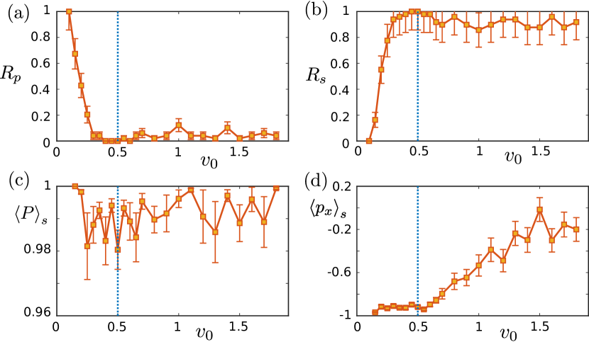
Figure 4: (a) Ratio of the finally pinned states $R_{p}$(lower bound) as a function of the particle velocity $v_{0}$. (b) Ratio of the finally sliding states $R_{s}$ (lower bound) as a function of the particle velocity $v_{0}$. (c) Average polarization of the bands in the finally sliding states $\left<P\right>_{s}$ as a function of $v_{0}$. (d) Average cosine of the bands $\left<p_{x}\right>_{s}$ in the finally sliding states as a function of $v_{0}$. The inset shows the respective standard deviation of ${p_{x}}…_{s}$ for the different realizations. Here we have used $g=0.07$, $D_{r}^{c}=0.15$, $N=5000$, $L_{x}=500$,$L_{y}=5$, $D_{r}=3\times 10^{-5}$, $u_{0}=0.3,\omega=0.02,k=0.1$ ($v_{L}=0.2$). The dotted vertical line marks the value of the velocity $v_{0}=0.5$ beyond which sliding in the positive direction is possible.

Complementary information about the finally sliding states, featuring a current reversal, is provided by Figs. 4 (c),(d). The final average polarization of these states $\left<P\right>_{s}$ is for all $v_{0}$ very close to 1 (Fig. 4 (c)), owing to the low noise which results in particles clustering to a macroband with a certain alignment. In contrast, the direction of this alignment, quantified by $\left<p_{x}\right>_{s}=\left<\cos\theta\right>_{s}$, is affected strongly by $v_{0}$ (Fig. 4 (d)). For $0.1<v_{0}\leq 0.5$ we have $\left<p_{x}\right>_{s}\approx-0.95$, indicating that within this interval the particles’ velocities are all approximately aligned towards $-\mathbf{e}_{x}$ (as in Fig. 3 (i)) and thus the particles counterpropagate at roughly their maximum velocity. This picture changes when $v_{0}>0.5$ where a sliding also in the forward direction becomes possible. Different realizations result in finally sliding states with a different alignment $\mathbf{p}_{i}$ and thus their ensemble average $\left<p_{x}\right>_{s}\rightarrow 0$ as $v_{0}$ increases, recovering the isotropy in the direction of sliding bands of the Vicsek model in the absence of a lattice.

VII Effect of the noise amplitude

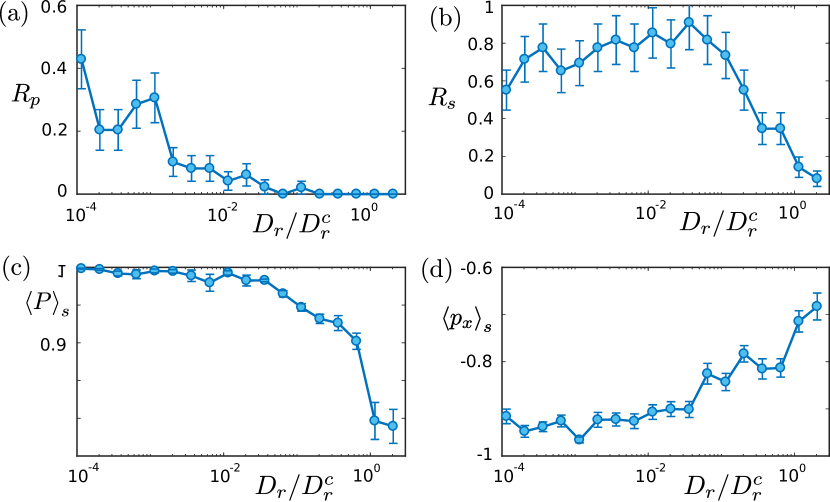
Figure 5: (a) Ratio of the finally pinned states $R_{p}$ (lower bound) as a function of the noise amplitude $D_{r}$ (in units of $D_{r}^{c}$). (b) Ratio of the finally sliding states $R_{s}$ (lower bound) as a function of the noise amplitude $D_{r}$ (in units of $D_{r}^{c}$). (c) Average polarization of the bands in the finally sliding states $\left<P\right>_{s}$ as a function of $D_{r}$. (d) Average cosine of the bands $\left<p_{x}\right>_{s}$ in the finally sliding states as a function of $D_{r}$. Here we have used $g=0.07$, $D_{r}^{c}=0.15$, $N=5000$, $L_{x}=500$,$L_{y}=5$, $v_{0}=0.2$, $u_{0}=0.3,\omega=0.02,k=0.1$ ($v_{L}=0.2$).

Rotational diffusion, whose strength is controlled by $D_{r}$, is crucial to initiate the emergence of sliding states; on the other hand, there is an upper critical noise strength $D_{r}^{c}$ above which the Vicsek model does not show polar order, but is in the isotropic phase. We now systematically explore how the transition to the counterpropagating macroband is affected when changing $D_{r}$. For $u_{0}=0.3,v_{0}=v_{L}=0.2$ where sliding is possible only in the negative $x$ direction, the ratio of states which are pinned at the end of our simulations $R_{p}$ decreases as $D_{r}$ increases (Fig. 5 (a)) and finally approaches zero for $D_{r}\gtrsim 0.1D_{r}^{c}$. The reason for this behaviour is probably that larger noise turns the orientation of the polarization of initially pinned bands faster and therefore initiates sliding earlier (and more often). The respective ratio of finally sliding states $R_{s}$ (Fig. 5 (b)) increases only slightly as $D_{r}$ increases from zero for $D_{r}\lesssim 0.05D_{r}^{c}$ and afterwards decreases tending towards zero. Physically, when $D_{r}$ is too large, the polarization of a band may significantly change between each subsequent collisions with other bands and may therefore leave the sliding regime before encountering another collision. Thus, for too strong noise, the emergence of a transition to a counterpropagating macroband is rather unlikely. The generic behaviour of the system for such high noise values is that of a mixture of individual particles, both in the pinned and in the sliding phase, whose polarization orientation changes fast in time, providing the picture of an overall disordered phase modulated by the existing potential wells (Figs. 6 (a),(b)). There is however still a possibility of obtaining a finally sliding state even in the high noise regime (Fig. 5 (b)). Such states are significantly less polarized than the ones in the low noise regime (Figs. 5 (c), 6 (c)) featuring also a larger variety in the direction of alignment, quantified by $\left<p_{x}\right>_{s}$ (Figs. 5 (d), 6 (d)). Furthermore, for such cases of high noise (e.g. $D_{r}=0.3$, $D_{r}=0.95$) the time evolution of both $\left<p_{x}\right>$ and $\left<P\right>$ is much slower (Figs. 6 (e),(f)) than the ones observed for lower noise values (e.g. $D_{r}=0.0003$, $D_{r}=0.003$), indicating the diffusive character of the dynamics expected for highly noisy systems.

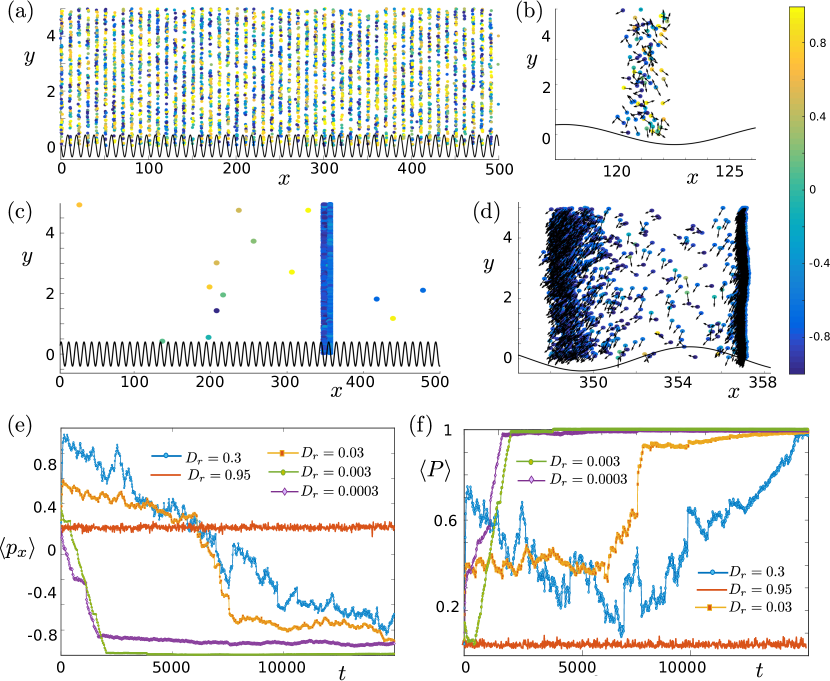
Figure 6: (a),(b) Snapshot of the pinned phase in the presence of a lattice from a sample simulation at high noise $D_{r}=0.95$ and a zoomed figure showing the orientation of the particles. (c),(d) Snapshot of the sliding phase in the presence of a lattice from a sample simulation at high noise $D_{r}=0.3$ and a zoomed figure showing the orientation of the particles. (e),(f) Time evolution of (a) the average cosine $\left<p_{x}\right>$ and (b) the average polarization $\left<P\right>$ for sample simulations leading to a finally sliding state for five different values of $D_{r}$. Note the difference of Figs (c),(d) from Fig. 2 (f).

VIII Conclusions

The present results provide a scheme allowing to control the typically highly irregular collective dynamics of polar active particles. In particular, we have seen that the bands occurring in the Vicsek model, which normally move in unpredictable directions and irregularly merge and split up can be tamed by applying a traveling wave-shaped potential, as can be realized e.g. using a micropatterned moving substrate or a traversing optical lattice. We find that while most particles in the system self-organize into polarized bands which comove with the lattice at early times, they can later experience a remarkable reversal, initiated by the counterpropagation of a single band which subsequently consumes all other bands in the system. The asymptotic state is a strongly polarized macroband which predictably moves opposite to the direction of the motion of the external substrate. This behaviour is representative in a large parameter window and can be controlled e.g. by tuning the relative speed of the active particles and the lattice. These results may inspire further research of the interface between nonlinear dynamics and active matter and perhaps also applications regarding collective targeted cargo delivery using polar active matter.

- [1] S Ramaswamy. The mechanics and statistics of active matter. Annu. Rev. Cond. Matt. Phys., 1.
- [2] M C Marchetti, J-F Joanny, S Ramaswamy, T B Liverpool, J Prost, M Rao, and R A Simha. Hydrodynamics of soft active matter. Rev. Mod. Phys., 85(3):1143, 2013.
- [3] Clemens Bechinger, Roberto Di Leonardo, Hartmut Löwen, Charles Reichhardt, Giorgio Volpe, and Giovanni Volpe. Active particles in complex and crowded environments. Rev. Mod. Phys., 88(4):045006, 2016.
- [4] I Theurkauff, C Cottin-Bizonne, J Palacci, C Ybert, and L Bocquet. Dynamic clustering in active colloidal suspensions with chemical signaling. Phys. Rev. Lett., 108(26):268303, 2012.
- [5] Jérémie Palacci, Stefano Sacanna, Adrian Vatchinsky, Paul M Chaikin, and David J Pine. Photoactivated colloidal dockers for cargo transportation. J. Am. Chem. Soc., 135(43):15978, 2013.
- [6] I Buttinoni, J Bialké, F Kümmel, H Löwen, C Bechinger, and T Speck. Dynamical clustering and phase separation in suspensions of self-propelled colloidal particles. Phys. Rev. Lett., 110(23):238301, 2013.
- [7] F Ginot, I Theurkauff, F Detcheverry, C Ybert, and C Cottin-Bizonne. Aggregation-fragmentation and individual dynamics of active clusters. Nature Comm., 9(1):696, 2018.
- [8] Benno Liebchen and Hartmut Löwen. Which interactions dominate in active colloids? arXiv preprint arXiv:1808.07389, 2018.
- [9] Rodrigo Soto and Ramin Golestanian. Self-assembly of catalytically active colloidal molecules: tailoring activity through surface chemistry. Phys. Rev. Lett., 112(6):068301, 2014.
- [10] Akhil Varma, Thomas D Montenegro-Johnson, and Sebastien Michelin. Clustering-induced self-propulsion of isotropic autophoretic particles. arXiv preprint arXiv:1806.03812, 2018.
- [11] Falko Schmidt, Benno Liebchen, Hartmut Löwen, and Giovanni Volpe. Light-controlled assembly of active colloidal molecules. arXiv preprint arXiv:1801.06868, 2018.
- [12] Andrey Sokolov and Igor S Aranson. Physical properties of collective motion in suspensions of bacteria. Phys. Rev. Lett., 109(24):248109, 2012.
- [13] Henricus H Wensink, Jörn Dunkel, Sebastian Heidenreich, Knut Drescher, Raymond E Goldstein, Hartmut Löwen, and Julia M Yeomans. Meso-scale turbulence in living fluids. Proc. Natl. Acad. Sci., 2012.
- [14] Andreas Kaiser, Anton Peshkov, Andrey Sokolov, Borge ten Hagen, Hartmut Löwen, and Igor S Aranson. Transport powered by bacterial turbulence. Phys. Rev. Lett., 112(15):158101, 2014.
- [15] Joakim Stenhammar, Cesare Nardini, Rupert W Nash, Davide Marenduzzo, and Alexander Morozov. Role of correlations in the collective behavior of microswimmer suspensions. Phys. Rev. Lett., 119(2):028005, 2017.
- [16] Ingmar H Riedel, Karsten Kruse, and Jonathon Howard. A self-organized vortex array of hydrodynamically entrained sperm cells. Science, 309(5732):300–303, 2005.
- [17] Martin Loose and Timothy J Mitchison. The bacterial cell division proteins ftsa and ftsz self-organize into dynamic cytoskeletal patterns. Nature Cell Biol., 16(1):38, 2014.
- [18] J Denk, L Huber, E Reithmann, and E Frey. Active curved polymers form vortex patterns on membranes. Phys. Rev. Lett., 116(17):178301, 2016.
- [19] Benno Liebchen and Demian Levis. Collective behavior of chiral active matter: pattern formation and enhanced flocking. Phys. Rev. Lett., 119(5):058002, 2017.
- [20] Volker Schaller, Christoph Weber, Christine Semmrich, Erwin Frey, and Andreas R Bausch. Polar patterns of driven filaments. Nature, 467(7311):73, 2010.
- [21] Thomas Le Goff, Benno Liebchen, and Davide Marenduzzo. Pattern formation in polymerizing actin flocks: Spirals, spots, and waves without nonlinear chemistry. Phys. Ref. Lett., 117(23):238002, 2016.
- [22] John Toner, Yuhai Tu, and Sriram Ramaswamy. Hydrodynamics and phases of flocks. Ann. Phys., 318(1):170–244, 2005.
- [23] Walter F Paxton, Kevin C Kistler, Christine C Olmeda, Ayusman Sen, Sarah K St. Angelo, Yanyan Cao, Thomas E Mallouk, Paul E Lammert, and Vincent H Crespi. Catalytic nanomotors: autonomous movement of striped nanorods. J. Am. Chem. Soc., 126(41):13424, 2004.
- [24] Fernando Peruani. Active brownian rods. Eur. Phys. J. Spec. Top., 225(11-12):2301, 2016.
- [25] J Toner and Y Tu. Long-range order in a two-dimensional dynamical xy model: how birds fly together. Phys. Rev. Lett., 75(23):4326, 1995.
- [26] N David Mermin and Herbert Wagner. Absence of ferromagnetism or antiferromagnetism in one-or two-dimensional isotropic heisenberg models. Phys. Rev. Lett., 17(22):1133, 1966.
- [27] G Grégoire and H Chaté. Onset of collective and cohesive motion. Phys. Rev. Lett., 92(2):025702, 2004.
- [28] Jean-Baptiste Caussin, Alexandre Solon, Anton Peshkov, Hugues Chaté, Thierry Dauxois, Julien Tailleur, Vincenzo Vitelli, and Denis Bartolo. Emergent spatial structures in flocking models: A dynamical system insight. Phys. Rev. Lett., 112:148102, Apr 2014.
- [29] Alexandre P Solon, Hugues Chaté, and Julien Tailleur. From phase to microphase separation in flocking models: The essential role of nonequilibrium fluctuations. Phys. Rev. Lett., 114(6):068101, 2015.
- [30] N Koumakis, A Lepore, C Maggi, and R Di Leonardo. Targeted delivery of colloids by swimming bacteria. Nat. Comm., 4:2588, 2013.
- [31] Xing Ma, Kersten Hahn, and Samuel Sanchez. Catalytic mesoporous janus nanomotors for active cargo delivery. J. Am. Chem. Soc., 137(15):4976, 2015.
- [32] SJ Ebbens. Active colloids: Progress and challenges towards realising autonomous applications. Curr. Opin. Colloid Interface Sci., 21:14–23, 2016.
- [33] Alexander Geiseler, Peter Hänggi, Fabio Marchesoni, Colm Mulhern, and Sergey Savel’ev. Chemotaxis of artificial microswimmers in active density waves. Phys. Rev. E, 94(1):012613, 2016.
- [34] Ahmet F Demirörs, Fritz Eichenseher, Martin J Loessner, and André R Studart. Colloidal shuttles for programmable cargo transport. Nat. Comm., 8(1):1872, 2017.
- [35] Simona Colabrese, Kristian Gustavsson, Antonio Celani, and Luca Biferale. Flow navigation by smart microswimmers via reinforcement learning. Phys. Rev. Lett., 118(15):158004, 2017.
- [36] Alexander Geiseler, Peter Hänggi, and Fabio Marchesoni. Self-polarizing microswimmers in active density waves. Sci. Rep., 7:41884, 2017.
- [37] Santiago Muiños-Landin, Keyan Ghazi-Zahedi, and Frank Cichos. Reinforcement learning of artificial microswimmers. arXiv preprint arXiv:1803.06425, 2018.
- [38] Jeffrey A Drocco, CJ Olson Reichhardt, and Cynthia Reichhardt. Bidirectional sorting of flocking particles in the presence of asymmetric barriers. Phys. Rev. E, 85(5):056102, 2012.
- [39] Félix Ginot, Isaac Theurkauff, Demian Levis, Christophe Ybert, Lydéric Bocquet, Ludovic Berthier, and Cécile Cottin-Bizonne. Nonequilibrium equation of state in suspensions of active colloids. Phys. Rev. X, 5(1):011004, 2015.
- [40] Jan-Timm Kuhr, Johannes Blaschke, Felix Rühle, and Holger Stark. Collective sedimentation of squirmers under gravity. Soft matter, 13(41):7548, 2017.
- [41] C Reichhardt and CJO Reichhardt. Negative differential mobility and trapping in active matter systems. J. Phys.: Cond. Matter, 30(1):015404, 2017.
- [42] Wei-jing Zhu, Xiao-qun Huang, and Bao-quan Ai. Transport of underdamped self-propelled particles in active density waves. J. Phys. A, 51(11):115101, 2018.
- [43] C Reichhardt and CJO Reichhardt. Clogging and depinning of ballistic active matter systems in disordered media. Phys. Rev. E, 97(5):052613, 2018.
- [44] Jing Yan, Ming Han, Jie Zhang, Cong Xu, Erik Luijten, and Steve Granick. Reconfiguring active particles by electrostatic imbalance. Nat. Mater., 15(10):1095, 2016.
- [45] Chenhui Peng, Taras Turiv, Yubing Guo, Qi-Huo Wei, and Oleg D Lavrentovich. Command of active matter by topological defects and patterns. Science, 354(6314):882, 2016.
- [46] Pau Guillamat, Jordi Ignés-Mullol, and Francesc Sagués. Control of active liquid crystals with a magnetic field. Proc. Natl. Acad. Sci., 113(20):5498, 2016.
- [47] Pau Guillamat, Jordi Ignés-Mullol, and Francesc Sagués. Taming active turbulence with patterned soft interfaces. Nat. Comm., 8(1):564, 2017.
- [48] Andreas Kaiser, Alexey Snezhko, and Igor S Aranson. Flocking ferromagnetic colloids. Sci. Adv., 3(2):e1601469, 2017.
- [49] Peter Reimann. Brownian motors: noisy transport far from equilibrium. Physics reports, 361(2-4):57–265, 2002.
- [50] Cs Sándor, Andras Libál, Charles Reichhardt, and CJ Olson Reichhardt. Collective transport for active matter run-and-tumble disk systems on a traveling-wave substrate. Phys. Rev. E, 95(1):012607, 2017.
- [51] Pietro Tierno and Arthur V Straube. Transport and selective chaining of bidisperse particles in a travelling wave potential. Eur. Phys. J. E, 39(5):54, 2016.
- [52] Peter Hänggi and Fabio Marchesoni. Artificial brownian motors: Controlling transport on the nanoscale. Rev. Mod. Phys., 81(1):387, 2009.
- [53] Michael PN Juniper, Arthur V Straube, Dirk GAL Aarts, and Roel PA Dullens. Colloidal particles driven across periodic optical-potential-energy landscapes. Phys. Rev. E, 93(1):012608, 2016.
- [54] Michael PN Juniper, Urs Zimmermann, Arthur V Straube, Rut Besseling, Dirk GAL Aarts, Hartmut Löwen, and Roel PA Dullens. Dynamic mode locking in a driven colloidal system: experiments and theory. New J. Phys., 19(1):013010, 2017.
- [55] Consider the dynamics of free, not fully overdamped particles yielding the solution , i.e. the timescale on which a particle reaches the velocity is . We assume here that this time scale is much shorter than all other time scales in the system, including those applied by the travelling wave potential.
- [56] Choosing length and time units as shows that the parameter space has five essential dimensions: the Peclet number measuring the persistence length of the active particles (in bulk) in units of the particle radius, the reduced alignment rate , comparing the typical alignment rate of the particles with the Brownian decay of alignment, the reduced lattice depth and the reduced frequency and wave vector of the lattice (and the density ). The mass unit is implicitly fixed as yielding an energy unit of , where we have used the Einstein and the Stokes-Einstein-Debye relation.
- [57] P Coullet, J. M Gilli, M Monticelli, and N Vandenberghe. A damped pendulum forced with a constant torque. Am. J. Phys., 73:1122, 2005.
- [58] O. M Braun and Y. S Kivshar. The Frenkel-Kontorova Model: Concepts, Methods and Applications. Springer, Berlin, 2004.
- [59] A Barone and G. Paternò. Physics and Applications of the Josephson Effect. Wiley & Sons, New York, 1982.
- [60] L Cheng and Yip N. K. The long time behavior of brownian motion in tilted periodic potentials. Physica D, 297:1, 2015.