Reconstruction of surfaces with ordinary singularities from their silhouettes^∗

Abstract.

We present algorithms for reconstructing, up to unavoidable projective automorphisms, surfaces with ordinary singularities in three dimensional space starting from their silhouette, or “apparent contour” — namely the branching locus of a projection on the plane — and the projection of their singular locus.

1. Introduction

In this paper, we provide an algorithm that deals with the following problem: given a homogeneous ternary polynomial $D$ which is the discriminant of a polynomial $F$, reconstruct $F$ up to unavoidable automorphisms of the polynomial ring that preserve the discriminant. We do not tackle this problem in its full generality, and to understand better the conditions that we impose on the polynomial $F$, it is useful to rephrase the question in a geometric setting. If we let $S$ be the surface in $\mathbb{P}^{3}$ defined by $F$, and we consider a linear projection $\mathbb{P}^{3}\dashrightarrow\mathbb{P}^{2}$, we call contour the locus of points in $S$ whose tangent space passes though the center of projection. The projection of the contour is the silhouette of $S$, and it is the zero set of the discriminant of $F$ in the direction given by the linear projection. The previous problem can then be specified as follows: given the silhouette of $S$ under a projection $\mathbb{P}^{3}\dashrightarrow\mathbb{P}^{2}$, we want to reconstruct the surface $S$ and the projection to $\mathbb{P}^{2}$. Since we can always precompose a projection by an automorphism of $\mathbb{P}^{3}$, we can only hope to solve the problem modulo these automorphisms. We restrict to surfaces that have at most ordinary singularities, namely those singularities that arise on a general projection to $\mathbb{P}^{3}$ of a smooth surface living in a higher dimensional projective space. Moreover, we suppose that all projections $\mathbb{P}^{3}\dashrightarrow\mathbb{P}^{2}$ we consider are have “good” properties, namely those that would arise by projecting from a general point. This implies that the silhouettes we consider have only “simple” singularities (see Figure 1).

In its geometric version, the problem we investigate comes within the field of algebraic vision, namely the study, via algebra and geometry, of problems from computer vision. This subject has been investigated intensively in the last years; see, for example, the books [13, 17] and, among others, the papers [23, 24, 20, 33, 34, 37]. In particular, the problem of reconstructing 3D shapes from 2D information has been investigated thoroughly (see for example [5], [22] and [21]). Attempting to reconstruct a 3D surface from just one 2D picture (namely, from its silhouette) seems hopeless because small bumps or perturbations in the direction of the camera do not leave any trace on the contour. There are situations where this approach was tried, but only when strong a priori knowledge about the object to reconstruct is available (see [32] and [40]). However, in the algebraic setting, this turns out to be doable, due to the rigidity of algebraic varieties. The question of reconstruction of a surface from its silhouette was investigated by the Italian school of algebraic geometry at the beginning of the twentieth century, and culminated with the formulation of Chisini’s conjecture and its solution by Kulikov in 1999.

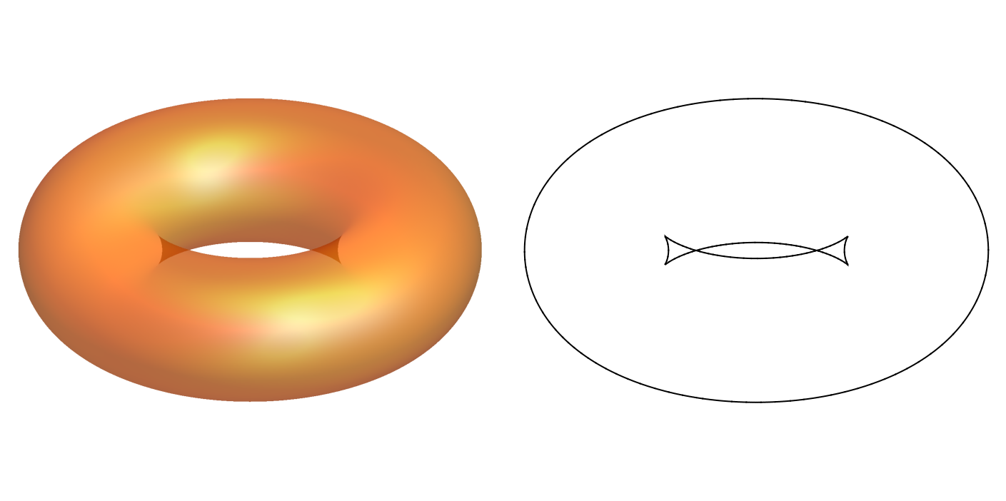
Figure 1. On the left, a ring torus, an algebraic surface of degree $4$. On the right, we highlight its silhouette.

Chisini’s conjecture

Following the works of Enriques (see [12] and related papers by Zariski [39] and Segre [35]), Chisini asked in [8] whether a surface can be reconstructed from its silhouette when it is projected to $\mathbb{P}^{2}$. In more modern terms, (see [6, Introduction, Definition 1]), one defines a multiple plane to be a pair $(S,f)$ where $S$ is a compact connected complex surface and $f$ is a finite holomorphic map $f\colon S\longrightarrow\mathbb{P}^{2}$. The pair $(S,f)$ is said to be general if the ramification divisor $R$ of $f$ is smooth and reduced, $f(R)=B$ has only nodes and ordinary cusps as singularities, and $f_{|_{R}}\colon R\longrightarrow B$ has degree $1$. Chisini conjectured that if two general multiple planes $(S,f)$ and $(S^{\prime},f^{\prime})$, whose maps have degree $\geq 5$, have the same branching locus $B\subset\mathbb{P}^{2}$, then there exists an isomorphism $\phi\colon S\longrightarrow S^{\prime}$ such that $f^{\prime}\circ\phi=f$. Several authors investigated this problem (see [6, 31, 27, 30] and [7, Section 7.4]), until Kulikov solved it in affirmative way in [25] and [26]. Interestingly, the case when $S$ is a smooth surface in $\mathbb{P}^{3}$ and $f$ is a general linear projection to $\mathbb{P}^{2}$ is also solved by Forsyth in [15].

Cubic surfaces

Cubic surfaces in $\mathbb{P}^{3}$ are a first non-trivial, though still simple enough, case of surface reconstruction from the silhouette. This case was studied by Zariski [39] and Segre [35], by Chisini and Manara [9], and by Biggiogero [2] (she later considered also the case of quartic surfaces in [3]); more recently, works focusing on the real situation appeared, see for example [29] and [14]. A cubic form $F$ can always be brought to Tschirnhaus form $F=w^{3}+A(x,y,z)w+B(x,y,z)$ via automorphisms of $\mathbb{P}^{3}$; its discriminant is $\Delta=-(4A^{3}+27B^{2})$. The task of reconstructing the surface $\{F=0\}$ from its silhouette is equivalent to reconstructing $A$ and $B$ from $\Delta$. Generically, the curve $\Delta$ has six cusps; there is a unique conic passing through those six points, which one proves must be $A$ (possibly up to some scalar multiple). Once $A$ is known, the cubic $B$ can be computed as follows: one selects a cubic $C$ in the ideal of the six points which is linearly independent from the three linear multiples of $A$; then, one makes an ansatz for $B$ of the form $\lambda C+L\cdot A$ where $\lambda\in\mathbb{C}$ and $L$ a linear polynomial, and imposes that $-\bigl{(}4A^{3}+27(\lambda C+L\cdot A)\bigr{)}$ equals the given discriminant.

Unfortunately, already for quartic surfaces the formula for the discriminant is more complicated, and does not allow a straightforward generalization of the procedure for cubics. Nevertheless, the algorithm described in Section 3 (and already known in the literature) provides a generalization of the one for cubics when we restrict to smooth surfaces. Going further, the algorithm we present in Section 4 applies to even more general situations.

Our contribution

In this paper, we provide a reconstruction algorithm for surfaces in $\mathbb{P}^{3}$ that have at most ordinary singularities, namely those singularities that inevitably arise when we project a smooth surface in $\mathbb{P}^{5}$ to $\mathbb{P}^{3}$. Section 2 discusses general projections of surfaces with ordinary singularities, and in particular describes the possible singularities of the silhouette of such projections recalling some well-known classical results.

As a warm-up, in Section 3 we recall the procedure for recovering a smooth surface from its silhouette (see [11]). We proceed in two steps: first, we reconstruct the contour from the silhouette, and then we determine the surface. The construction of the contour is based on the fact that there is exactly one form $G_{1}$ of degree $d^{2}-3d+2$ vanishing at the singularities of the silhouette (in analogy with the existence of the conic $A$ in the situation of cubic surfaces); moreover, there is exactly one form $G_{2}$ of degree $d^{2}-3d+3$ vanishing at the singularities of the silhouette that is independent from $G_{1}$. The contour is the image of the silhouette under the rational map

$$(x:y:z)\;\mapsto\;(x:y:z:G_{2}/G_{1})\,.$$

Once the contour is known, the equation $F$ of the surface is determined so that $F$ and $\partial_{w}F$ generate the ideal of the contour (supposing that the projection is the one along the $w$-axis).

The algorithm for good projections of surfaces with ordinary singularities generalizes the one for smooth surfaces. Also here, we use the singularities of the silhouette in order to define a rational map that determines the contour as the image of the silhouette; after that, the reconstruction of the surface proceeds exactly as in the smooth situation. One important difference with the smooth case is that when dealing with surfaces with ordinary singularities we have to take into account the non-reduced structure of both the contour and the silhouette. Sheaf theory provides a firm theoretical ground to prove the correctness of our algorithm, which relies on a well-known formula relating the dualizing sheaves of the contour and of the silhouette.

While in the smooth case it is well-known that reconstruction is essentially unique, our algorithm could (and in some example really does) give finitely many essentially different results. The reason is that the two components of the silhouette, which are the projections of the curve of smooth points of the surface that are in the contour, and of the singular curve of the surface, may intersect transversally; these intersections may either be projections of pinch points, or just the result of two distinct points on the surface being collapsed by the projection, and it is not possible to distinguish these two situations by using only local analytic equations. This ambiguity is related to the failure of Chisini’s conjecture in low degree (see [6]). Figure 2 shows three essentially different Roman surfaces with the same silhouette; in this case, there are projective isomorphisms between the surfaces, but none of them preserves the center of projection. This case is discussed in more detail in Example 4.15.

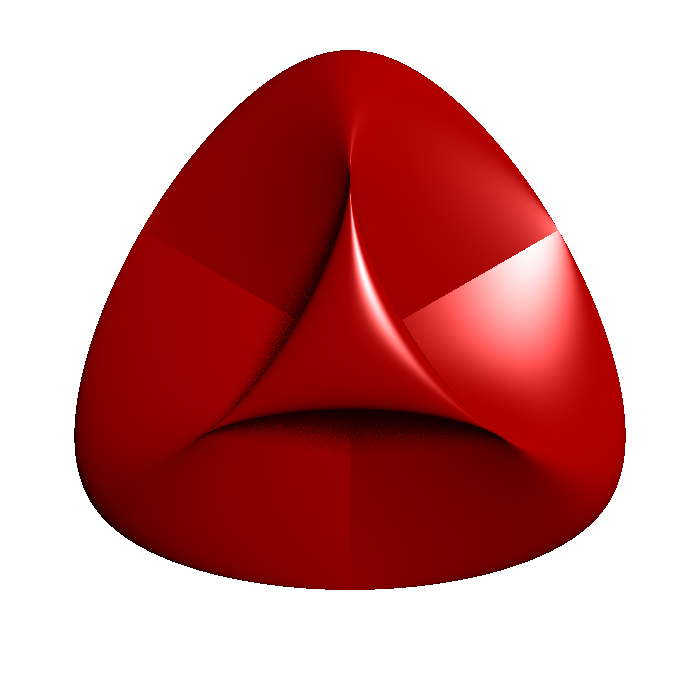
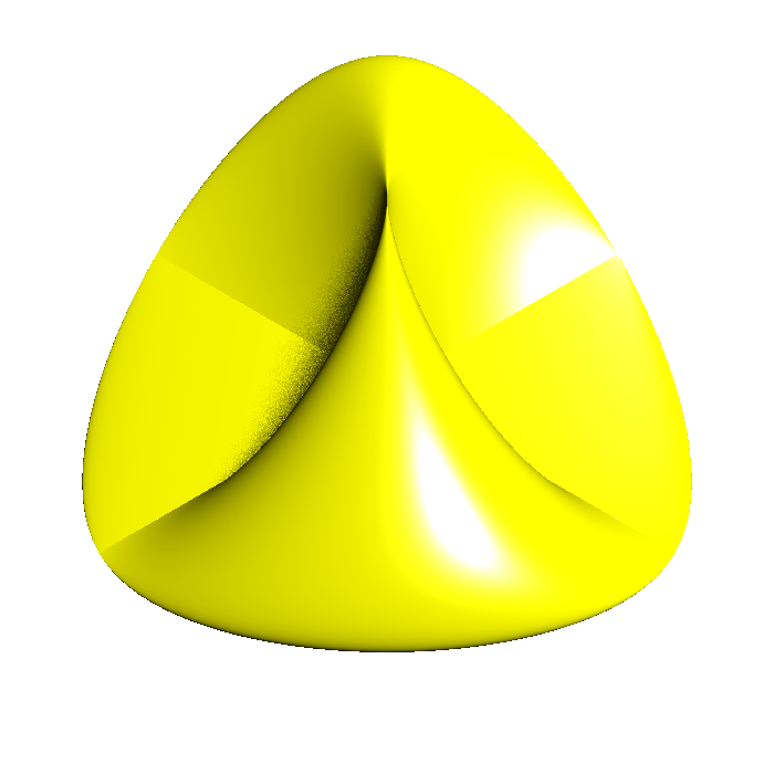
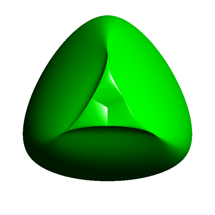
Figure 2. Three Roman surfaces with the same silhouette.

Concerning the algorithm

An implementation in Maple of our algorithm is available at

https://www.risc.jku.at/people/jschicho/pub/Chisini.mpl.

The algorithm can easily be re-implemented in any computer algebra system that provides Gröbner bases. We tested the program for randomly generated surfaces with different type of singularities of degree up to $6$; the performances are reported at the end of Section 4.

We tried to state the algorithm with as few references to the theory we used to prove its correctness as possible, in order to make it available to a wide range of readers. The proof of its correctness, instead, requires a basic knowledge of sheaf and scheme theory.

The package contains also symbolic proofs that are needed in Appendix A.

2. Singularities of surfaces and their contours and silhouettes

In this section we describe the kind of surfaces and projections we are going to deal with for the rest of the paper. We fix the following terminology. The contour of a surface $S\subset\mathbb{P}^{3}$ is the common zero set of the equation of the surface and its derivative in the direction of the projection. The contour is then the union of the singular locus $Z$ of $S$ and the proper contour $R\subset S$, namely the curve of smooth points of the surface whose tangent planes pass through the center of projection (see [10, Remark 3.3]).

The silhouette is the projection of the contour, and hence it is the union of the singular image $W\subset\mathbb{P}^{2}$, the projection of the singular locus, and of the proper silhouette $B\subset\mathbb{P}^{2}$, the projection of the proper contour. If the surface is smooth, the proper contour and the proper silhouette are, respectively, what in algebraic geometry are called the ramification locus and the branching locus of the projection $S\longrightarrow\mathbb{P}^{2}$ (see [10, Section 3.1]).

In our work, we consider surfaces $S\subset\mathbb{P}^{3}$ with ordinary singularities (see [28, Definition 7] and [10, Section 2.1]). Surfaces with ordinary singularities are surfaces whose only singularities are self-intersection curves (double curves), self-intersection triple points and pinch points (see Figure 3). Notice that, in particular, these surfaces cannot be tangent developables (this will be useful in the proof of Proposition 2.1). Moreover, our object of investigation will be good projections $S\longrightarrow\mathbb{P}^{2}$. A good projection is a linear map $S\longrightarrow\mathbb{P}^{2}$ where $S$ has ordinary singularities and such that:

1. the restriction of the projection to the contour is injective, except for at most finitely many points;

2. the proper contour $R$ is smooth, and the proper silhouette $B$ has at most nodes and ordinary cusps;

3. the line through the center of projection and a point in the proper contour $R$ intersects $S$ with multiplicity exactly $2$ at that point, except for preimages of cusps and singular points on the surface;

4. the singular image $W$ has only nodes and ordinary triple points ($D_{4}$ singularities), the latter arising as images of spatial triple points;

5. the singular image $W$ and the proper silhouette $B$ meet either transversally, or tangentially with order $2$ at smooth points; in particular, we ask pinch points to be mapped to transversal intersections.

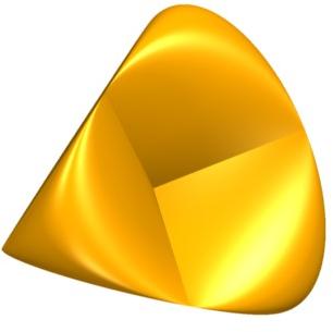
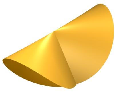
Figure 3. Examples of general singularities of a surface: on the left a self-intersection triple point and three pinch points (in a Roman surface) and on the right a pinch point (in a Whitney umbrella).

We remark that the assumptions on the singularities of the surfaces are satisfied if the surfaces are general projections of smooth surfaces (see [28, Theorem 8]).

We show now that the properties of good projections $S\longrightarrow\mathbb{P}^{2}$ are satisfied if we project a surface with ordinary singularities from a general point in $\mathbb{P}^{3}$. This is a mild generalization of [10, Theorem 1.2], and in several parts of the proof we use the same techniques used by Ciliberto and Flamini. In the proof, we use some auxiliary results (Lemmas 2.3, 2.4, 2.5 and 2.6) which are proved at the end of the section to increase readability since the proof of Proposition 2.1 is rather long.

Proposition 2.1.

If $S\subset\mathbb{P}^{3}$ is a surface with ordinary singularities, then the projection $S\longrightarrow\mathbb{P}^{2}$ from a general point $p\in\mathbb{P}^{3}$ is good.

Proof.

By [10, Theorem 1.2], properties (1), (2), and (3) hold for projections from a general center. By assumption, the singular curve $Z\subset S$ has no singularities other than triple points; a general projection may introduce at most nodes and project the spatial triple points to planar ordinary triple points. Hence condition (4) is satisfied.

In order to ensure condition (5), we start by showing that no singular point of the singular image $W\subset\mathbb{P}^{2}$ lies on the proper silhouette $B\subset\mathbb{P}^{2}$, and vice versa.

No triple point of the singular image $W$ lies on $B$. If the center of projection does not lie on any of the three tangent planes at any triple point of $Z$, then the contour does not pass through any triple point of $Z$. If we now consider the projection of $S$ from a triple point, this map has itself a silhouette curve, and the cone over this silhouette curve is constituted of lines that pass through the triple point and are tangent to $S$. We get finitely many such cones considering all triple points, and if the projection center is chosen outside the union of all of them, then no triple point of $W$ lies on the proper silhouette $B$.

If a node of the singular image $W$ lies in $B$, then the projection center must lie on a two-secant line of $Z$ which is tangent to the surface $S$ at a smooth point. Lemma 2.3 states that this does not happen for general projection centers, since these lines do not fill $\mathbb{P}^{3}$. Recall that, having ordinary singularities, the surface $S$ cannot be a tangent developable, and so we can use Lemma 2.3 and the subsequent result. By the way, a two-secant line of $Z$ that is tangent at a singular point of $S$ would be a trisecant of $Z$, hence lead to a triple point of $W$ not arising from a triple point of $Z$. This would contradict the first paragraph of the proof.

If a node of $B$ lies on $W$, then the projection center lies on a bitangent of $S$ that intersects $Z$. Lemma 2.4 excludes that happens for general projection centers.

If a cusp of $B$ lies on $W$, then the projection center must lie on an asymptotic tangent line (see [10, Section 3.2]) that intersects $Z$. Lemma 2.5 states that this does not happen for general projection centers.

We have established that $B$ and $W$ intersect only at points that are smooth in both curves. These intersections arise in two ways: projections of an intersection point of $Z$ and $R$, or projections of two distinct points, one smooth in $Z$ and another smooth in $R$. We show that $B$ and $W$ intersect transversally in both cases.

Suppose that the intersection is a projection of two distinct points. If the intersection were not transversal, then the center of projection would lie on a line $L$ that intersects $Z$ at a smooth point $q$ and such that the tangent to $Z$ at $q$ is contained in a tangent plane of $S$ at a smooth point contained in $L$. This is excluded by Lemma 2.6.

Suppose that the intersection of $B$ and $W$ comes from an intersection of $R$ and $Z$. The strategy here to show that $B$ and $W$ intersect transversally is the following: we first show that the intersection between $R$ and $Z$ must be transversal; then $R\cap Z$ can be either a simple double point of $R\cup Z$, or a pinch point. In the first case, we show that the point is mapped to a point of simple tangency; in the second case, we prove that the transversality of the intersection is preserved by the projection.

We begin with the first step, namely showing that the intersection between $R$ and $Z$ is transversal. We start by analyzing the tangent directions of the proper contour. Suppose that the surface $S$ is defined by a polynomial $F\in\mathbb{C}[x,y,z,w]$. Then the contour is defined by $F$ and by the polynomial $aF_{x}+bF_{y}+cF_{z}+dF_{w}$ where $(a:b:c:d)$ is the center of projection. If we de-homogenize setting $w=d=1$, then the equations for the contour are

$$F=0,\quad(x-a)F_{x}+(y-b)F_{y}+(z-c)F_{z}=0\,.$$

The tangent direction of the contour at $(x,y,z)$ is then given by the vector product of the gradients of the two equations:

$$\begin{pmatrix}F_{x}\\ F_{y}\\ F_{z}\end{pmatrix}\times\begin{pmatrix}F_{x}+(x-a)F_{xx}+(y-b)F_{xy}+(z-c)F_{xz}\\ F_{y}+(x-a)F_{yx}+(y-b)F_{yy}+(z-c)F_{yz}\\ F_{z}+(x-a)F_{zx}+(y-b)F_{zy}+(z-c)F_{zz}\end{pmatrix}=\\ =\nabla(F)\times\Bigl{(}H(F)\cdot\bigl{(}(x,y,z)-(a,b,c)\bigr{)}\Bigr{)}\,.$$

Let $P$ be an intersection point of $Z$ and $R$. Notice that the surface $S$ has two (analytic) branches around $P$. From now on, we focus the branch of the surface $S$ at $P$ containing the proper contour $R$, and we want to understand when the proper contour $R$ of $S$ is tangent to the singular locus $Z$. Hence, from now on we let $F$ denote the analytic equation of the branch of $S$ at $P$ that contains $R$. By a linear change of coordinates, we can assume that $P=(0,0,0)$ and $\nabla(F)|_{P}=(0,0,1)$, and that the tangent line $T_{P}Z$ is spanned by $(1,0,0)$. Locally at $P$, the affine equation of the branch of $S$ containing the proper contour is of the form $F(x,y,z)=z-f(x,y)$; moreover the center of the projection has coordinates $(a,b,0)$, otherwise the proper contour would not pass through $P$. Then

$$H(F)=\begin{pmatrix}f_{xx}&f_{xy}&0\\ f_{xy}&f_{yy}&0\\ 0&0&0\end{pmatrix}\,.$$

The direction of the contour at $P$ is then

$$\begin{pmatrix}0\\ 0\\ 1\end{pmatrix}\times\begin{pmatrix}f_{xx}\cdot a+f_{xy}\cdot b\\ f_{xy}\cdot a+f_{yy}\cdot b\\ 0\end{pmatrix}\,.$$

Hence the proper contour is tangent to the singular locus at $P$ if and only if

$$a\,f_{xx}+bf_{xy}=0\,,$$

since we supposed that the tangent direction of $Z$ at $P$ is $(1,0,0)$. We distinguish three situations:

$\mathrm{rk}\bigl{(}H(f)\bigr{)}=0$:

in this case the tangency condition is satisfied for every $(a,b)$.

$\mathrm{rk}\bigl{(}H(f)\bigr{)}=1$:

in this case we have a so-called parabolic point; the Hessian of $f$ is of the form $\left(\begin{smallmatrix}\alpha^{2}&\alpha\beta\\ \alpha\beta&\beta^{2}\end{smallmatrix}\right)$, and so it has a one-dimensional kernel, also called the asymptotic direction of the parabolic point. If the tangent direction of $Z$ lies in this kernel, then the tangency condition is satisfied for every $(a,b)$.

$\mathrm{rk}\bigl{(}H(f)\bigr{)}=2$:

in this case the tangency condition is not satisfied for a general choice of $(a,b)$.

We consider points with zero Hessian as degenerate parabolic points with infinitely many asymptotic directions, to avoid a case distinction in the rest of the proof. We claim that a curve of parabolic points, whose tangent direction is always the/a asymptotic direction, has the property that the tangent plane is constant along the curve. Recall that, locally, the surface has equation $z-f(x,y)=0$. We can locally define the curve by an additional second equation $y-h(x)=0$. We want to show that the gradient vector

$$\begin{pmatrix}f_{x}\bigl{(}x,h(x)\bigr{)}\\ f_{y}\bigl{(}x,h(x)\bigr{)}\\ -1\end{pmatrix}$$

is constant. The derivative of this expression is

$$\begin{pmatrix}f_{xx}\bigl{(}x,h(x)\bigr{)}+f_{xy}\bigl{(}x,h(x)\bigr{)}h^{\prime}(x)\\ f_{xy}\bigl{(}x,h(x)\bigr{)}+f_{yy}\bigl{(}x,h(x)\bigr{)}h^{\prime}(x)\\ 0\end{pmatrix}=\begin{pmatrix}H(f)\bigl{(}x,h(x)\bigr{)}\begin{pmatrix}1\\ h^{\prime}(x)\end{pmatrix}\\ 0\end{pmatrix}\,,$$

which is zero by assumption. The claim, namely the fact that the tangent plane is constant along the curve, is thus proven. Notice that, since as we already remarked a surface with ordinary singularities cannot be a tangent developable, not all points on the surface are parabolic. Hence, if the center of projection is outside these finitely many planes determined by curves of parabolic points or isolated parabolic points, the curves $R$ and $Z$ will intersect transversally.

We now show that if a point of intersection of $R$ and $Z$ is a pinch point, then its projection is a point of transverse intersection between $B$ and $W$; moreover, we show that if an intersection of $R$ and $Z$ is not a pinch point, then its projection is a point of simple tangential intersection of $B$ and $W$. Once we prove this, condition (5) is ensured and the whole proof is concluded.

Suppose that $P\in R\cap Z$ is not a pinch point. Locally around $P$, we can take analytic coordinates such that the proper contour is defined by $x=z=0$, the branch of $S$ containing it has equation $x-z^{2}=0$, and the projection is along the $z$-axis. Since $R$ and $Z$ intersect transversally, there exists a power series $h$ of positive order such that the equation of the singular locus $Z$ is of the form $y-h(z)=x-z^{2}=0$. The equation of the proper silhouette is $x=0$. The equation of the singular image is given by eliminating $z$ from the equations $y-h(z)=0$ and $x-z^{2}=0$. We write $h(z)$ in the form $zh_{1}(z^{2})+z^{2}h_{2}(z^{2})$, so the elimination ideal is generated by

$$\bigl{(}y+xh_{2}(x)\bigr{)}^{2}-xh_{1}(x)^{2}\,.$$

This shows that $B$ and $W$ have the same linear factor, so they are tangent, but if we set $x=0$ in the equation of $W$ we obtain a non-zero quadratic summand, proving that the tangency is simple.

Consider now the case that $P\in R\cap Z$ is a pinch point. Recall that a pinch point is a singular point such that the analytic germ of the surface at the point has equation equivalent to $z^{2}-yx^{2}=0$, see [10, Definition 2.1]. We know that pinch points are double points. Hence, for a general projection for which we choose coordinates $(x,y,z)\mapsto(x,y)$, we have that $S$ has local equation at $P$ of the form $z^{2}+h_{1}(x,y)z+h_{2}(x,y)=0$. A Tschirnhaus transformation $z\mapsto z-h_{1}(x,y)/2$, which leaves the direction of projection invariant, makes the local equation of $S$ in the form $z^{2}+h(x,y)=0$. Now, pinch points can be characterized as points such that the discriminant of a general projection is the product of a square of a linear factor and another linear factor intersecting transversally the first one, namely it is of the form $u^{2}v$. In these coordinates, hence, the surface $S$ has equation $z^{2}+u^{2}v=0$ at $P$, and the projection can still be assumed to be along the $z$-axis. The contour is then given by $z^{2}+u^{2}v=z=0$, so we see that the projection maps it isomorphically to the plane curve $u^{2}v=0$. This concludes the proof that pinch points project to transverse intersections of the proper silhouette and the singular image. ∎

In order to prove the auxiliary results needed for Proposition 2.1 we use the results from focal geometry introduced and proved in [10, Sections 4 and 5]. Here we briefly sketch the setting and the results, and we refer to the work of Ciliberto and Flamini for more precise information. We consider families of lines in $\mathbb{P}^{3}$, namely varieties $\mathscr{X}\subset D\times\mathbb{P}^{3}$, where $D\subset\mathbb{G}(1,3)$ is a subvariety of the Grassmannian of lines in $\mathbb{P}^{3}$, of the form

$$\mathscr{X}=\bigl{\{}(\delta,x)\,\colon\,\delta\in D,\,x\text{ belongs to the line corresponding to }\delta\bigr{\}}\,.$$

By restricting the second projection to $\mathscr{X}$, we get a map $f\colon\mathscr{X}\longrightarrow\mathbb{P}^{3}$; its ramification points form the focal locus of $\mathscr{X}$. We say that $\mathscr{X}$ is a filling family if $D$ is two-dimensional and $f$ is dominant.

Theorem 2.2.

Let $f\colon\mathscr{X}\longrightarrow\mathbb{P}^{3}$ be a filling family, let $S\subset\mathbb{P}^{3}$ be a non-developable surface, and let $Z\subset\mathbb{P}^{3}$ be a curve. For a general element $\delta\in D$, the fiber

$$\mathscr{X}_{\delta}=\bigl{\{}(\delta,x)\in\mathscr{X}\,\colon\,x\text{ belongs to the line corresponding to }\delta\bigr{\}}$$

intersects the focal locus in two points (or one counted with multiplicity $2$).

Moreover, if for a general element $\delta\in D$ the line $\ell=f(\mathscr{X}_{\delta})$ intersects the surface $S$ tangentially at a point $p$, then the following properties hold:

• the point $(\delta,p)\in\mathscr{X}_{\delta}$ is a focus, namely a point in the focal locus;

• the multiplicity of intersection of $\ell$ with $S$ at $p$ is at most $3$;

• if the multiplicity of intersection of $\ell$ with $S$ at $p$ is $3$, then $(\delta,p)$ is a focus of $\mathscr{X}_{\delta}$ of multiplicity $2$.

Moreover, if for a general element $\delta\in D$ the line $\ell=f(\mathscr{X}_{\delta})$ intersects the curve $Z$ in a point $p$, then $(\delta,p)$ is a focus in $\mathscr{X}_{\delta}$.

Notice that the last statement in Theorem 2.2 is not present in [10] but can be proven in an analogous way. Moreover, in [10] it is used the notion of contact order instead of multiplicity of intersection: however, these two numbers just differ by $1$, so we adopt the latter notion.

With these results at hand, we can proceed with proving our auxiliary lemmas. Here, the considered families of lines $\mathscr{X}$ are families whose general element is tangent or bitangent to a given non-developable surface $S$ and intersects a given curve $Z$.

Lemma 2.3.

Let $S\subset\mathbb{P}^{3}$ be a non-developable surface and let $Z\subset\mathbb{P}^{3}$ be a curve. Then the family of two-secant lines of $Z$ that are tangent to the surface $S$ at a smooth point does not fill $\mathbb{P}^{3}$.

Proof.

If such a family were filling, then any of its general members would carry three foci, which is impossible by Theorem 2.2. ∎

Lemma 2.4.

Let $S\subset\mathbb{P}^{3}$ be a non-developable surface and let $Z\subset\mathbb{P}^{3}$ be a curve. Then the family of bitangents of $S$ that intersect $Z$ does not fill $\mathbb{P}^{3}$.

Proof.

If such a family were filling, then any of its general members would carry three foci, which is impossible by Theorem 2.2. ∎

Lemma 2.5.

Let $S\subset\mathbb{P}^{3}$ be a non-developable surface and let $Z\subset\mathbb{P}^{3}$ be a curve. Then the family of asymptotic tangent lines of $S$ that intersect $Z$ does not fill $\mathbb{P}^{3}$.

Proof.

If such a family were filling, then any of its general members would carry two foci, one of which with multiplicity $2$, which is impossible by Theorem 2.2. ∎

Lemma 2.6.

Let $S\subset\mathbb{P}^{3}$ be a non-developable surface and let $Z\subset\mathbb{P}^{3}$ be a curve. Then the family of lines $L$ that intersect $Z$ at a smooth point $q$ and such that the tangent to $Z$ at $q$ is contained in a tangent plane of $S$ at a smooth point contained in $L$ does not fill $\mathbb{P}^{3}$.

Proof.

Assume indirectly that the family of lines is filling. Let $\mathscr{Y}$ be the family of tangent planes to $S$ whose existence is postulated by the assumption (these planes have to be tangent to $Z$ as well). We distinguish two cases. First, suppose that $\mathscr{Y}$ is two-dimensional. The family $\mathscr{Y}$ is contained in the two-dimensional family of tangent planes to $S$, and in the two-dimensional family of tangent planes to $Z$, and both families are irreducible. Moreover, the second family forms a tangent developable surface in the dual projective space, while the first one does not. So the two irreducible families cannot be equal and therefore intersect in a family of dimension one, which contradicts the assumption. Second, suppose that $\mathscr{Y}$ is one-dimensional. Then there are infinitely many lines of the filling family contained in a general plane in $\mathscr{Y}$. It follows that there are infinitely many points at which such a plane is tangent to $S$. Then the surface $S$ has only a one-dimensional family of tangent planes, which implies that it is a developable surface. This contradicts the assumption. ∎

To sum up, suppose we have a good projection $S\longrightarrow\mathbb{P}^{2}$. If $B$ is the proper silhouette and $W$ is the singular image of the surface $S$, then the curve $B\cup W$ has only the following $7$ types of singularities, which we call special points (see Figure 4):

• nodes or cusps of $B$,

• nodes or triple points of $W$,

• tangential intersections of $B$ and $W$,

• transversal intersections of $B$ and $W$ whose preimages are distinct,

• transversal intersections of $B$ and $W$ coming from pinch points.

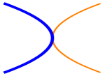
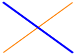
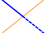
Figure 4. The seven possible singularities of the union of the proper silhouette (thinner, in orange) and the singular image (thicker, in blue) of a surface in $\mathbb{P}^{3}$. The case of a singularity coming from a pinch point of the surface is denoted by a dotted line.

3. Reconstruction of smooth surfaces

The question of reconstructing a smooth surface from its silhouette has been answered by d’Almeida in [11]. We report his construction — without any claim of originality — because it introduces several key concepts that will be used later in Section 4 to deal with the more general case of surfaces with ordinary singularities.

The silhouette of a good projection of a smooth surface in $\mathbb{P}^{3}$ of degree $d$ is a curve of degree $d(d-1)$ with only nodes and cusps as singularities (see Figure 5). The contour, also of degree $d(d-1)$, is a smooth curve which is a complete intersection and hence it is linearly normal, namely it is not the projection of a non-degenerate curve living in a bigger projective space. Therefore, we can reconstruct the contour from the silhouette as its linear normalization (see [38, Definition 2.11]). Once we have access to the ideal of the contour, the unique form of degree $d-1$ must be the derivative in the direction of the projection of the yet to-be-determined equation of the surface. Finding such an equation becomes then a problem in linear algebra, which admits a unique solution.

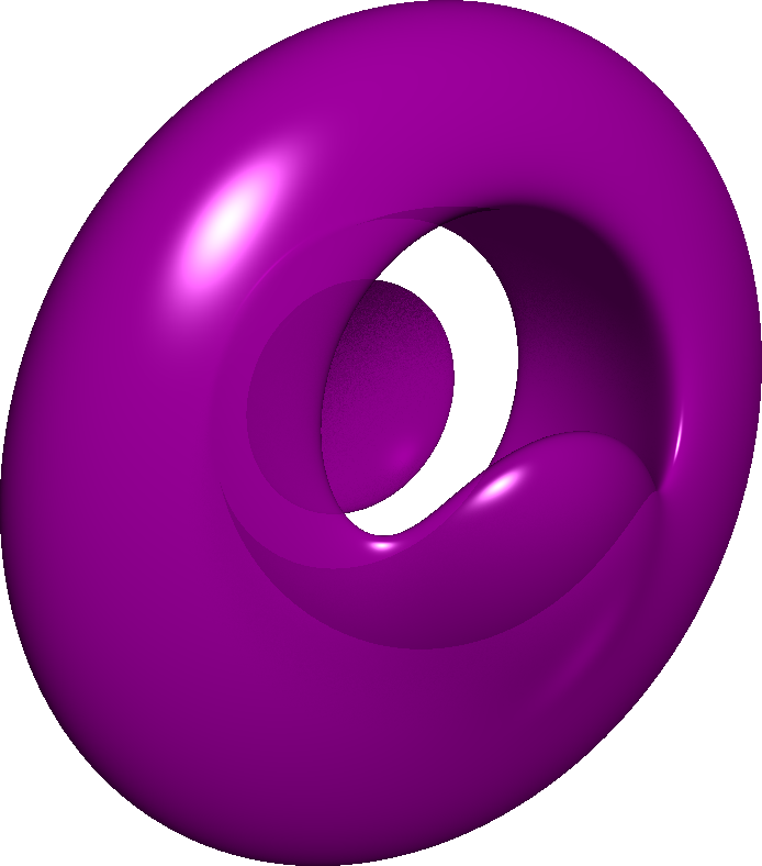
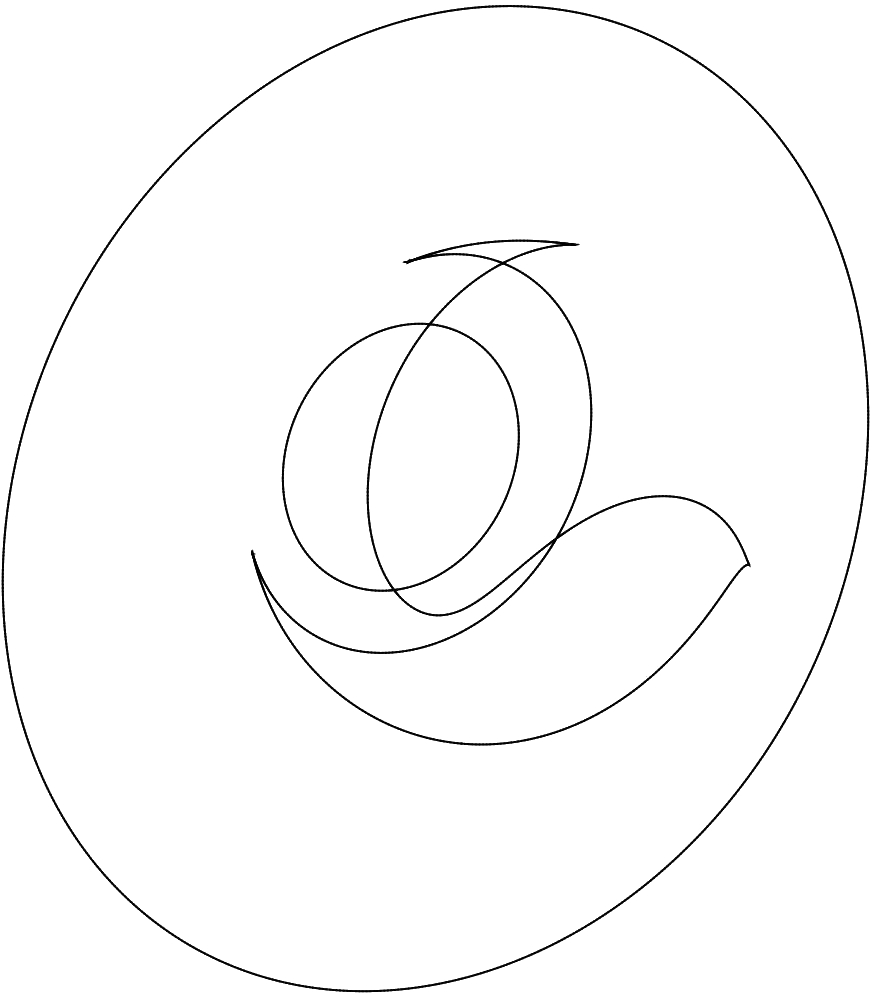
Figure 5. A smooth surface of degree $4$ (on the left) and its silhouette in the plane (on the right).

We start by the reconstruction of the contour.

Remark 3.1.

The key fact here is that $\mathscr{O}_{R}(1)$, the line bundle embedding the contour $R$ in $\mathbb{P}^{3}$, is a twist of the canonical sheaf $\omega_{R}$ of $R$; by the theory of adjoints, one proves that $\pi_{\ast}(\omega_{R})$ is a twist of the ideal of singularities of the silhouette $B$. The global sections of $\pi_{\ast}\mathscr{O}_{R}(1)$ can then be obtained as homogeneous forms of a certain degree passing through the singularities of $B$. In this way we get a way to map $B$ into $\mathbb{P}^{3}$ whose image is projectively equivalent to $R$.

Lemma 3.2.

The contour $R$ of a good projection is linearly normal. This means that the standard map $\operatorname{H}^{0}\bigl{(}\mathbb{P}^{3},\mathscr{O}_{\mathbb{P}^{3}}(1)\bigr{)}\longrightarrow\operatorname{H}^{0}\bigl{(}R,\mathscr{O}_{R}(1)\bigr{)}$ is an isomorphism. In particular, $\operatorname{H}^{0}\bigl{(}R,\mathscr{O}_{R}(1)\bigr{)}$ is $4$-dimensional.

Proof.

Since $R$ is a smooth complete intersection, it is linearly normal. ∎

Lemma 3.3.

The canonical sheaf $\omega_{R}$ of $R$ is isomorphic to $\mathscr{O}_{R}(2d-5)$. Moreover, the canonical sheaf $\omega_{B}=\pi_{\ast}(\omega_{R})$ of the silhouette $B$ is isomorphic to $\mathscr{J}\bigl{(}d^{2}-d-3\bigr{)}$, where $\mathscr{J}$ is the restriction to $B$ of the ideal sheaf $\mathscr{K}$ on $\mathbb{P}^{2}$ of the singularities of $B$.

Proof.

The statement regarding the canonical sheaf of $R$ follows from the fact that $R$ is the complete intersection of two surfaces of degree $d$ and $d-1$, and from the adjunction formula, see [18, Exercise II.8.4e]. Since $B$ has degree $d(d-1)$, the theory of adjoints for plane curves shows that

$$\omega_{B}\cong\mathscr{J}\bigl{(}d(d-1)-3\bigr{)}=\mathscr{J}\bigl{(}d^{2}-d-3\bigr{)}\,,$$

see [16, Chapter 8, Proposition 8] for the case of curves with only nodes, the situation of cusps is analogous. ∎

Proposition 3.4.

The complete linear series $|\omega_{B}(-2d+6)|$ maps $B$ to $\mathbb{P}^{3}$, and the image of this map is, up to projective equivalence in $\mathbb{P}^{3}$ over $B$, equal to $R$. These linear series correspond to global sections of $\mathscr{J}(d^{2}-3d+3)$.

Proof.

We showed in Lemma 3.3 that there is an isomorphism $\omega_{R}(-2d+6)\cong\mathscr{O}_{R}(1)$. Recall that the latter divisor is the one providing the embedding of the contour $R$ in $\mathbb{P}^{3}$, and in this embedding $R$ is linearly normal. The projection $R\longrightarrow B$ determines an isomorphism between the global sections of $\omega_{R}$ and $\omega_{B}$. By construction, the image of $B$ under the complete linear series $|\omega_{B}(-2d+6)|$ is also linearly normal, and so must coincide up to projective equivalence over $B$ with $R$. The last statement follows from the second part of Lemma 3.3. ∎

Since $\omega_{R}(-2d+6)\cong\mathscr{O}_{R}(1)$, it follows that $\operatorname{h}^{0}\bigl{(}\omega_{R}(-2d+6)\bigr{)}=4$. Thus, there are exactly $4$ linearly independent forms of degree $d^{2}-3d+3$ in the ideal $J$ defining the sheaf $\mathscr{J}$. Since $\omega_{R}(-2d+5)\cong\mathscr{O}_{R}$, it follows that $\omega_{B}(-2d+5)\cong\mathscr{O}_{B}$, and so $\mathscr{J}(d^{2}-3d+2)$ has a one-dimensional space of global sections.

Notice that for all $n\in\mathbb{N}$ there is the following exact sequence:

$$\lx@xy@svg{\hbox{\raise 0.0pt\hbox{\kern 5.5pt\hbox{\ignorespaces\ignorespaces\ignorespaces\hbox{\vtop{\kern 0.0pt\offinterlineskip\halign{\entry@#!@&&\entry@@#!@\cr&&&&\crcr}}}\ignorespaces{\hbox{\kern-5.5pt\raise 0.0pt\hbox{\hbox{\kern 0.0pt\raise 0.0pt\hbox{\hbox{\kern 3.0pt\raise 0.0pt\hbox{$\textstyle{0\ignorespaces\ignorespaces\ignorespaces\ignorespaces}$}}}}}}}\ignorespaces\ignorespaces\ignorespaces\ignorespaces{}{\hbox{\lx@xy@droprule}}\ignorespaces{\hbox{\kern 29.5pt\raise 0.0pt\hbox{\hbox{\kern 0.0pt\raise 0.0pt\hbox{\lx@xy@tip{1}\lx@xy@tip{-1}}}}}}{\hbox{\lx@xy@droprule}}{\hbox{\lx@xy@droprule}}{\hbox{\kern 29.5pt\raise 0.0pt\hbox{\hbox{\kern 0.0pt\raise 0.0pt\hbox{\hbox{\kern 3.0pt\raise 0.0pt\hbox{$\textstyle{\mathscr{I}(n)\ignorespaces\ignorespaces\ignorespaces\ignorespaces}$}}}}}}}\ignorespaces\ignorespaces\ignorespaces\ignorespaces{}{\hbox{\lx@xy@droprule}}\ignorespaces{\hbox{\kern 76.89127pt\raise 0.0pt\hbox{\hbox{\kern 0.0pt\raise 0.0pt\hbox{\lx@xy@tip{1}\lx@xy@tip{-1}}}}}}{\hbox{\lx@xy@droprule}}{\hbox{\lx@xy@droprule}}{\hbox{\kern 76.89127pt\raise 0.0pt\hbox{\hbox{\kern 0.0pt\raise 0.0pt\hbox{\hbox{\kern 3.0pt\raise 0.0pt\hbox{$\textstyle{\mathscr{K}(n)\ignorespaces\ignorespaces\ignorespaces\ignorespaces}$}}}}}}}\ignorespaces\ignorespaces\ignorespaces\ignorespaces{}{\hbox{\lx@xy@droprule}}\ignorespaces{\hbox{\kern 128.44922pt\raise 0.0pt\hbox{\hbox{\kern 0.0pt\raise 0.0pt\hbox{\lx@xy@tip{1}\lx@xy@tip{-1}}}}}}{\hbox{\lx@xy@droprule}}{\hbox{\lx@xy@droprule}}{\hbox{\kern 128.44922pt\raise 0.0pt\hbox{\hbox{\kern 0.0pt\raise 0.0pt\hbox{\hbox{\kern 3.0pt\raise 0.0pt\hbox{$\textstyle{\mathscr{J}(n)\ignorespaces\ignorespaces\ignorespaces\ignorespaces}$}}}}}}}\ignorespaces\ignorespaces\ignorespaces\ignorespaces{}{\hbox{\lx@xy@droprule}}\ignorespaces{\hbox{\kern 177.36826pt\raise 0.0pt\hbox{\hbox{\kern 0.0pt\raise 0.0pt\hbox{\lx@xy@tip{1}\lx@xy@tip{-1}}}}}}{\hbox{\lx@xy@droprule}}{\hbox{\lx@xy@droprule}}{\hbox{\kern 177.36826pt\raise 0.0pt\hbox{\hbox{\kern 0.0pt\raise 0.0pt\hbox{\hbox{\kern 3.0pt\raise 0.0pt\hbox{$\textstyle{0}$}}}}}}}\ignorespaces}}}}\ignorespaces\,, \textstyle{0\ignorespaces\ignorespaces\ignorespaces\ignorespaces} \textstyle{\mathscr{I}(n)\ignorespaces\ignorespaces\ignorespaces\ignorespaces} \textstyle{\mathscr{K}(n)\ignorespaces\ignorespaces\ignorespaces\ignorespaces} \textstyle{\mathscr{J}(n)\ignorespaces\ignorespaces\ignorespaces\ignorespaces} \textstyle{0} \textstyle{0\ignorespaces\ignorespaces\ignorespaces\ignorespaces} \textstyle{\mathscr{I}(n)\ignorespaces\ignorespaces\ignorespaces\ignorespaces} \textstyle{\mathscr{K}(n)\ignorespaces\ignorespaces\ignorespaces\ignorespaces} \textstyle{\mathscr{J}(n)\ignorespaces\ignorespaces\ignorespaces\ignorespaces} \textstyle{0}$$

where $\mathscr{I}$ is the ideal sheaf of $B$ on $\mathbb{P}^{2}$. Taking global sections, we get:

$$\lx@xy@svg{\hbox{\raise 0.0pt\hbox{\kern 5.5pt\hbox{\ignorespaces\ignorespaces\ignorespaces\hbox{\vtop{\kern 0.0pt\offinterlineskip\halign{\entry@#!@&&\entry@@#!@\cr&&&&\crcr}}}\ignorespaces{\hbox{\kern-5.5pt\raise 0.0pt\hbox{\hbox{\kern 0.0pt\raise 0.0pt\hbox{\hbox{\kern 3.0pt\raise 0.0pt\hbox{$\textstyle{0\ignorespaces\ignorespaces\ignorespaces\ignorespaces}$}}}}}}}\ignorespaces\ignorespaces\ignorespaces\ignorespaces{}{\hbox{\lx@xy@droprule}}\ignorespaces{\hbox{\kern 29.5pt\raise 0.0pt\hbox{\hbox{\kern 0.0pt\raise 0.0pt\hbox{\lx@xy@tip{1}\lx@xy@tip{-1}}}}}}{\hbox{\lx@xy@droprule}}{\hbox{\lx@xy@droprule}}{\hbox{\kern 29.5pt\raise 0.0pt\hbox{\hbox{\kern 0.0pt\raise 0.0pt\hbox{\hbox{\kern 3.0pt\raise 0.0pt\hbox{$\textstyle{\operatorname{H}^{0}\bigl{(}\mathscr{I}(n)\bigr{)}\ignorespaces\ignorespaces\ignorespaces\ignorespaces}$}}}}}}}\ignorespaces\ignorespaces\ignorespaces\ignorespaces{}{\hbox{\lx@xy@droprule}}\ignorespaces{\hbox{\kern 96.52463pt\raise 0.0pt\hbox{\hbox{\kern 0.0pt\raise 0.0pt\hbox{\lx@xy@tip{1}\lx@xy@tip{-1}}}}}}{\hbox{\lx@xy@droprule}}{\hbox{\lx@xy@droprule}}{\hbox{\kern 96.52463pt\raise 0.0pt\hbox{\hbox{\kern 0.0pt\raise 0.0pt\hbox{\hbox{\kern 3.0pt\raise 0.0pt\hbox{$\textstyle{\operatorname{H}^{0}\bigl{(}\mathscr{K}(n)\bigr{)}\ignorespaces\ignorespaces\ignorespaces\ignorespaces}$}}}}}}}\ignorespaces\ignorespaces\ignorespaces\ignorespaces{}{\hbox{\lx@xy@droprule}}\ignorespaces{\hbox{\kern 167.71594pt\raise 0.0pt\hbox{\hbox{\kern 0.0pt\raise 0.0pt\hbox{\lx@xy@tip{1}\lx@xy@tip{-1}}}}}}{\hbox{\lx@xy@droprule}}{\hbox{\lx@xy@droprule}}{\hbox{\kern 167.71594pt\raise 0.0pt\hbox{\hbox{\kern 0.0pt\raise 0.0pt\hbox{\hbox{\kern 3.0pt\raise 0.0pt\hbox{$\textstyle{\operatorname{H}^{0}\bigl{(}\mathscr{J}(n)\bigr{)}\ignorespaces\ignorespaces\ignorespaces\ignorespaces}$}}}}}}}\ignorespaces\ignorespaces\ignorespaces\ignorespaces{}{\hbox{\lx@xy@droprule}}\ignorespaces{\hbox{\kern 236.26834pt\raise 0.0pt\hbox{\hbox{\kern 0.0pt\raise 0.0pt\hbox{\lx@xy@tip{1}\lx@xy@tip{-1}}}}}}{\hbox{\lx@xy@droprule}}{\hbox{\lx@xy@droprule}}{\hbox{\kern 236.26834pt\raise 0.0pt\hbox{\hbox{\kern 0.0pt\raise 0.0pt\hbox{\hbox{\kern 3.0pt\raise 0.0pt\hbox{$\textstyle{\operatorname{H}^{1}\bigl{(}\mathscr{I}(n)\bigr{)}}$}}}}}}}\ignorespaces}}}}\ignorespaces\,. \textstyle{0\ignorespaces\ignorespaces\ignorespaces\ignorespaces} \textstyle{\operatorname{H}^{0}\bigl{(}\mathscr{I}(n)\bigr{)}\ignorespaces\ignorespaces\ignorespaces\ignorespaces} \textstyle{\operatorname{H}^{0}\bigl{(}\mathscr{K}(n)\bigr{)}\ignorespaces\ignorespaces\ignorespaces\ignorespaces} \textstyle{\operatorname{H}^{0}\bigl{(}\mathscr{J}(n)\bigr{)}\ignorespaces\ignorespaces\ignorespaces\ignorespaces} \textstyle{\operatorname{H}^{1}\bigl{(}\mathscr{I}(n)\bigr{)}} \textstyle{0\ignorespaces\ignorespaces\ignorespaces\ignorespaces} \textstyle{\operatorname{H}^{0}\bigl{(}\mathscr{I}(n)\bigr{)}\ignorespaces\ignorespaces\ignorespaces\ignorespaces} \textstyle{\operatorname{H}^{0}\bigl{(}\mathscr{K}(n)\bigr{)}\ignorespaces\ignorespaces\ignorespaces\ignorespaces} \textstyle{\operatorname{H}^{0}\bigl{(}\mathscr{J}(n)\bigr{)}\ignorespaces\ignorespaces\ignorespaces\ignorespaces} \textstyle{\operatorname{H}^{1}\bigl{(}\mathscr{I}(n)\bigr{)}}$$

Since $B$ has degree $d(d-1)$, we have $\mathscr{I}(n)\cong\mathscr{O}_{\mathbb{P}^{2}}(-d(d-1)+n)$. It follows that $\operatorname{H}^{1}\bigl{(}\mathscr{I}(n)\bigr{)}=0$ for all $n\in\mathbb{N}$. Thus, global sections of $\mathscr{J}(n)$ are restrictions of global sections of $\mathscr{K}(n)$ in $\mathbb{P}^{2}$. Hence there exists a unique (up to scalars) form $G_{1}$ of degree $d^{2}-3d+2$ in the ideal $K$ of singularities of $B$, and there is a unique form $G_{2}$ of degree $d^{2}-3d+3$ up to scalars and multiples of $G_{1}$.

Proposition 3.4 implies that the contour $R$ can be obtained by mapping the silhouette $B$ via the rational map from $\mathbb{P}^{2}$ to $\mathbb{P}^{3}$ given by three multiples of $G_{1}$ by linearly independent linear forms, and $G_{2}$, see Steps $2$ and $3$ in Algorithm ReconstructSmoothSurface. If we take coordinates so that the projection $S\longrightarrow\mathbb{P}^{2}$ is the map forgetting the last coordinate, then the three linear forms can be taken to be $x$, $y$ and $z$; in this way, the rational map $\mathbb{P}^{2}\dashrightarrow\mathbb{P}^{3}$ is

$$(x:y:z)\mapsto(x:y:z:G_{2}/G_{1})$$

and it is a section of the projection, see Step $4$ of Algorithm ReconstructSmoothSurface.

Once the contour is reconstructed, let $I$ be its homogeneous ideal in $\mathbb{C}[x,y,z,w]$. By hypothesis, the minimal non-zero homogeneous component of $I$ is the one in degree $d-1$. This component is one-dimensional, hence the derivative $H$ of the equation of the surface in the direction of the projection is uniquely determined up to scalars. Now, it is enough to compute a form $F$ of degree $d$ in $I$ such that its derivative is $H$. This amounts to solving a system of linear equations, see Steps $5$ and $6$ of Algorithm ReconstructSmoothSurface. In fact, suppose that the projection direction is the one along the $w$-axis; by integration we can compute a primitive $\widetilde{H}$ of $H$; then we make an ansatz for the integration constant, which must be a homogeneous polynomial $N$ of degree $d$ depending only on $x$, $y$ and $z$. Reducing the polynomial $\widetilde{H}+N$ modulo a Gröbner basis of $I$ gives linear equations for the coefficients of $N$.

Claim. This linear system has a unique solution.

Proof. Suppose that $F_{1}$ and $F_{2}$ are two different solutions; then there are constants $a$ and $b$ such that $F:=aF_{1}+bF_{2}$ is an element of $I$ such that its derivative along the direction of the projection is zero. This means that $F$ is the equation of a cone of degree $d$ passing through the contour $R$ whose vertex is the projection center. The projection of the cone would be a component of degree $d$ of the silhouette. This is absurd because the silhouette is irreducible of degree $d(d-1)$. $\square$

This proves that Algorithm ReconstructSmoothSurface is correct and that every smooth surface having branching locus $B$ is projectively equivalent over $B$ to the output.

Algorithm 1 ReconstructSmoothSurface

1:A curve $B\subset\mathbb{P}^{2}$, the silhouette of a good projection to $\mathbb{P}^{2}$ of a smooth surface $S\subset\mathbb{P}^{3}$ of degree $d$.

2:A smooth surface $S\subset\mathbb{P}^{3}$ together with a projection to $\mathbb{P}^{2}$ such that $B$ is the branching locus of this projection.

3:

4:Compute the radical $K$ of the Jacobian ideal of $B$.

5:Select in $K$ a form $G_{1}$ of degree $d^{2}-3d+2$.

6:Select in $K$ a form $G_{2}$ of degree $d^{2}-3d+3$ which is not a multiple of $G_{1}$.

7:Compute the ideal $I$ of the image $R$ of $B$ under the map

$$(x:y:z)\mapsto(x:y:z:G_{2}/G_{1}).$$

8:Select in $I$ a form $H$ of degree $d-1$.

9:Select in $I$ a form $F$ whose derivative is a scalar multiple of $H$.

10:Return $F$.

4. Reconstruction of surfaces with ordinary singularities

In this section we present a reconstruction algorithm for good projections $S\longrightarrow\mathbb{P}^{2}$. It subsumes the previous case presented in Section 3. The idea is similar to the one in the smooth case: we first reconstruct the contour, and then we obtain the surface via linear algebra. However, now it is not enough to compute the normalization of the silhouette, because the contour may be singular. Instead, we solve local reconstruction problems for each of the seven types of special points that can arise in the silhouette and obtain the global result by sheaf theory.

Recall that we denote by $Z$ the singular locus of $S$ and by $R$ the proper contour of a good projection; moreover, we denote by $W$ the singular image, and by $B$ the proper silhouette. For our purposes, the set-theoretic description of the contour is insufficient, so we define two scheme-theoretic notions.

Definition 4.1.

The fat contour $Y$ is the one-dimensional scheme defined by the equation of surface $S$ and its derivative in the direction of the projection. This scheme is supported on the set $Z\cup R$.

The fat silhouette $C$ is the one-dimensional scheme defined by the discriminant of the equation of the surface. This scheme is supported on the set $W\cup B$.

Proposition 4.2.

A good projection maps $Y$ onto $C$ and it is an isomorphism except over the special points of $C$.

Proof.

Since the projection is good, it is injective except over the special points. The component of $Y$ supported on $R$ is reduced because of the hypothesis that tangent lines through the center of projection intersect the surface with multiplicity $2$ at contour points. Hence the set-theoretic isomorphism implies scheme-theoretic isomorphism for those points. This is not immediately the case for the component of $Y$ supported on $Z$. Locally at a smooth point of $Z$ outside the contour, the surface $S$ is analytically isomorphic to $z(z-x)=0$, the fat contour $Y$ is defined by $2z-x=z(z-x)=0$, and $C$ is defined by $x^{2}=0$; hence the restriction of the projection to $Y$ is an isomorphism (of schemes) with inverse described by the homomorphism of rings $\mathbb{C}[x,y,z]/(2z-x,z(z-x))\longrightarrow\mathbb{C}[x,y]/(x^{2})$ given by $([x],[y],[z])\mapsto([x],[y],[x/2])$. ∎

The strategy for reconstructing the fat contour of a good projection from the fat silhouette mimics the one in the smooth case. First of all, we express the sheaf $\mathscr{O}_{Y}(1)$, which provides the embedding of $Y$ in $\mathbb{P}^{3}$, as a twist of the dualizing sheaf $\omega^{\circ}_{Y}$, which is a substitute in the non-smooth setting for the canonical sheaf. Using the “upper shriek” operation, in Lemmas 4.4 and 4.5 we connect the dualizing sheaves of $Y$ and $C$, and obtain that in order to determine the direct image of $\mathscr{O}_{Y}(1)$ under a projection $\pi$, it is enough to compute (a twist of) the sheaf $\mathscr{H}\!\!om_{\mathscr{O}_{C}}\bigl{(}\pi_{\ast}\mathscr{O}_{Y},\mathscr{O}_{C}\bigr{)}$, which is supported at the special points of $C$. The latter comes with a natural map to $\mathscr{O}_{C}$, and we show that this map is injective, proving that $\mathscr{H}\!\!om_{\mathscr{O}_{C}}\bigl{(}\pi_{\ast}\mathscr{O}_{Y},\mathscr{O}_{C}\bigr{)}$ is an ideal sheaf. Therefore, the problem of determining a rational map sending $C$ to $Y$ becomes equivalent to the computation of the space of homogeneous forms of a certain degree that satisfy particular vanishing conditions at the special points of $C$. This is analogous to the smooth situation, where we computed the adjoint forms of the silhouette.

Recall that a crucial step in the smooth situation is the fact that the contour $R$ is linearly normal, or equivalently (for smooth varieties) that the standard map $\operatorname{H}^{0}\bigl{(}\mathbb{P}^{3},\mathscr{O}_{\mathbb{P}^{3}}(1)\bigr{)}\longrightarrow\operatorname{H}^{0}\bigl{(}R,\mathscr{O}_{Y}(1)\bigr{)}$ is an isomorphism. We prove that the latter condition holds also for the fat contour, which is very far from being smooth.

Lemma 4.3.

The map $\operatorname{H}^{0}\bigl{(}\mathbb{P}^{3},\mathscr{O}_{\mathbb{P}^{3}}(1)\bigr{)}\longrightarrow\operatorname{H}^{0}\bigl{(}Y,\mathscr{O}_{Y}(1)\bigr{)}$ is an isomorphism. In particular, $\operatorname{H}^{0}\bigl{(}Y,\mathscr{O}_{Y}(1)\bigr{)}$ is $4$-dimensional.

Proof.

This follows from the fact that $Y$ is a complete intersection of two surfaces of degree $d$ and $d-1$, and so we have a graded free resolution of $\mathscr{O}_{Y}$ provided by the Koszul complex:

Twisting by $\mathscr{O}_{Y}(1)$ and looking at the corresponding long exact sequence in cohomology yields the result. ∎

We now show how to reconstruct the fat contour $Y$ and the projection $\pi_{|_{Y}}\colon Y\longrightarrow C$ starting from the fat silhouette $C$. As pointed out at the beginning of the section, this is carried out locally, and the local data are patched together using the fact that both schemes, being projective over a field, admit a dualizing sheaf $\omega^{\circ}$ (see [18, Proposition III.7.5]).

In particular, in our case we have:

Lemma 4.4.

$\omega_{Y}^{\circ}\cong\mathscr{O}_{Y}(2d-5)$ and $\omega_{C}^{\circ}\cong\mathscr{O}_{C}(d^{2}-d-3)$.

Proof.

For a closed subscheme $X$ of $\mathbb{P}^{n}$ that is a local complete intersection of codimension $r$, we have by [18, Theorem III.7.11]

$$\omega_{X}^{\circ}\cong\omega_{\mathbb{P}^{n}}\otimes\bigwedge^{r}\bigl{(}\mathscr{I}/\mathscr{I}^{2}\bigr{)}^{\vee}\,,$$

where $\mathscr{I}$ is the ideal sheaf of $X$, and $(\cdot)^{\vee}$ denotes the dual sheaf. The claim follows from this formula and the definitions of $Y$ and $C$ as complete intersections. ∎

If we think of $Y$ as an abstract scheme, it is embedded in $\mathbb{P}^{3}$ via morphism determined by the global sections of the sheaf $\mathscr{O}_{Y}(1)$. Since our goal, as in the smooth situation, is to compute a map from $C$ to $\mathbb{P}^{3}$ whose image gives $Y$, we link the global sections of $\mathscr{O}_{Y}(1)$ to the ones of a sheaf on $C$.

Lemma 4.5.

$\operatorname{H}^{0}\bigl{(}Y,\mathscr{O}_{Y}(1)\bigr{)}\cong\operatorname{H}^{0}\Bigl{(}C,\mathscr{H}\!\!om_{\mathscr{O}_{C}}\bigl{(}\pi_{\ast}\mathscr{O}_{Y},\mathscr{O}_{C}\bigr{)}(d^{2}-3d+3)\Bigr{)}$.

Proof.

Since the projection $\pi_{|_{Y}}\colon Y\longrightarrow C$ is a finite affine morphism, we have that $\omega_{Y}^{\circ}=\pi^{!}\bigl{(}\omega_{C}^{\circ}\bigr{)}$ by [18, Exercise III.7.2]. The sheaf $\pi^{!}\bigl{(}\omega_{C}^{\circ}\bigr{)}$, called “$\pi$ upper shriek” is defined in the following way (see [18, Exercise III.6.10]). The sheaf $\mathscr{H}\!\!om_{\mathscr{O}_{C}}\bigl{(}\pi_{\ast}\mathscr{O}_{Y},\omega_{C}^{\circ}\bigr{)}$ is both an $\mathscr{O}_{C}$-module and a $\pi_{\ast}\mathscr{O}_{Y}$-module. For affine morphisms there is a correspondence between $\pi_{\ast}\mathscr{O}_{Y}$-modules and $\mathscr{O}_{Y}$-modules (see [18, Exercise II.5.17e]); the $\mathscr{O}_{Y}$-module corresponding to $\mathscr{H}\!\!om_{\mathscr{O}_{C}}\bigl{(}\pi_{\ast}\mathscr{O}_{Y},\omega_{C}^{\circ}\bigr{)}$ is defined to be $\pi^{!}\bigl{(}\omega_{C}^{\circ}\bigr{)}$. From Lemma 4.4 we get

$$\operatorname{H}^{0}\bigl{(}Y,\mathscr{O}_{Y}(1)\bigr{)} \cong\operatorname{H}^{0}\bigl{(}Y,\omega_{Y}^{\circ}(-2d+6)\bigr{)}$$

$$\cong\operatorname{H}^{0}\bigl{(}Y,\pi^{!}(\omega_{C}^{\circ})(-2d+6)\bigr{)}$$

$$\cong\operatorname{H}^{0}\Bigl{(}C,\pi_{\ast}\bigl{(}\pi^{!}(\omega_{C}^{\circ})(-2d+6)\bigl{)}\Bigr{)}$$

$$\cong\operatorname{H}^{0}\Bigl{(}C,\pi_{\ast}\bigl{(}\pi^{!}(\omega_{C}^{\circ})\bigl{)}(-2d+6)\Bigr{)}\,,$$

where the latter isomorphism is given by the projection formula (see [18, Exercise II.5.1d]). By analyzing the correspondence between $\pi_{\ast}\mathscr{O}_{Y}$-modules and $\mathscr{O}_{Y}$-modules as hinted in [18, Exercise II.5.17e], one sees that $\pi_{\ast}\bigl{(}\pi^{!}(\omega_{C}^{\circ})\bigl{)}$ is $\mathscr{H}\!\!om_{\mathscr{O}_{C}}\bigl{(}\pi_{\ast}\mathscr{O}_{Y},\omega_{C}^{\circ}\bigr{)}$ as an $\mathscr{O}_{C}$-module. So we have

$$\operatorname{H}^{0}\bigl{(}Y,\mathscr{O}_{Y}(1)\bigr{)} \cong\operatorname{H}^{0}\Bigl{(}C,\mathscr{H}\!\!om_{\mathscr{O}_{C}}\bigl{(}\pi_{\ast}\mathscr{O}_{Y},\omega_{C}^{\circ}\bigr{)}(-2d+6)\Bigr{)}$$

$$\cong\operatorname{H}^{0}\Bigl{(}C,\mathscr{H}\!\!om_{\mathscr{O}_{C}}\bigl{(}\pi_{\ast}\mathscr{O}_{Y},\mathscr{O}_{C}(d^{2}-d-3)\bigr{)}(-2d+6)\Bigr{)}$$

$$\cong\operatorname{H}^{0}\Bigl{(}C,\mathscr{H}\!\!om_{\mathscr{O}_{C}}\bigl{(}\pi_{\ast}\mathscr{O}_{Y},\mathscr{O}_{C}\bigr{)}(d^{2}-3d+3)\Bigr{)}\,.$$

Notice that $\mathscr{H}\!\!om_{\mathscr{O}_{C}}\bigl{(}\pi_{\ast}\mathscr{O}_{Y},\mathscr{O}_{C}\bigr{)}$ is supported at the singularities of $C$ since by Proposition 4.2 a good projection is an isomorphism outside them. ∎

We are going to show that $\mathscr{H}\!\!om_{\mathscr{O}_{C}}\bigl{(}\pi_{\ast}\mathscr{O}_{Y},\mathscr{O}_{C}\bigr{)}$ is an ideal sheaf. We then compute the graded part of degree $d^{2}-3d+3$ of this ideal. By Lemma 4.5, a basis of this graded part provides a rational map from $C$ to $\mathbb{P}^{3}$ defined everywhere except at the special points (namely, the singularities of the silhouette); the image of this rational map is an open subscheme $Y^{\circ}$ of $Y$ intersecting both of its components nontrivially. The equation of the surface $S$ is then the only polynomial of degree $d$ vanishing on $Y^{\circ}$ such that its derivative in the direction of the projection also vanishes on $Y^{\circ}$, and this is what we compute in Algorithm ReconstructGeneralSurface.

Proposition 4.6.

The $\mathscr{O}_{C}$-module $\mathscr{H}\!\!om_{\mathscr{O}_{C}}\bigl{(}\pi_{\ast}\mathscr{O}_{Y},\mathscr{O}_{C}\bigr{)}$ is an ideal sheaf.

Proof.

There is a natural morphism of sheaves $\Phi\colon\mathscr{H}\!\!om_{\mathscr{O}_{C}}\bigl{(}\pi_{\ast}\mathscr{O}_{Y},\mathscr{O}_{C}\bigr{)}\longrightarrow\mathscr{O}_{C}$ sending a homomorphism $\varphi$ to $\varphi(1)$. We prove that $\Phi$ is injective, this showing that $\mathscr{H}\!\!om_{\mathscr{O}_{C}}\bigl{(}\pi_{\ast}\mathscr{O}_{Y},\mathscr{O}_{C}\bigr{)}$ is an ideal sheaf. To do so, it is enough to show that for every closed point $c\in C$, the induced map $\Phi_{c}\colon\mathscr{H}\!\!om_{\mathscr{O}_{C}}\bigl{(}\pi_{\ast}\mathscr{O}_{Y},\mathscr{O}_{C}\bigr{)}_{c}\longrightarrow\mathscr{O}_{C,c}$ on stalks is injective. In turn, we can pass to the completion, namely we can tensor by $\widehat{\mathscr{O}}_{C,c}$, and prove injectivity in that case, since the completion of a local Noetherian ring is faithfully flat (see [36, Tag/00MC, Lemma 10.96.3]). Since the formation of $\operatorname{Hom}$ commutes with flat base change (see [36, Tag/087R, Remark 15.60.20]), it suffices to prove that the map

$$\widehat{\Phi}_{c}\colon\operatorname{Hom}_{\widehat{\mathscr{O}}_{C,c}}\bigl{(}(\pi_{\ast}\mathscr{O}_{Y})_{c}\otimes\widehat{\mathscr{O}}_{C,c},\widehat{\mathscr{O}}_{C,c}\bigr{)}\longrightarrow\widehat{\mathscr{O}}_{C,c}$$

is injective. Notice that the $\widehat{\mathscr{O}}_{C,c}$-module $(\pi_{\ast}\mathscr{O}_{Y})_{c}\otimes\widehat{\mathscr{O}}_{C,c}$ is isomorphic to the direct sum $\displaystyle\bigoplus_{y_{i}\colon\pi(y_{i})=c}\widehat{\mathscr{O}}_{Y,y_{i}}$. In fact, by the Theorem on Formal Functions (see [18, Theorem III.11.1 and Remark III.11.1.2]) we have that

$$(\pi_{\ast}\mathscr{O}_{Y})_{c}\otimes\widehat{\mathscr{O}}_{C,c}\;\cong\;\operatorname{H}^{0}\bigl{(}\widehat{Y},\mathscr{O}_{\widehat{Y}}\bigr{)}\,.$$

where $(\widehat{Y},\mathscr{O}_{\widehat{Y}})$ is the completion of $Y$ along $\pi^{-1}(c)$ (see [18, Definition III.9.3]). As a topological space, $\widehat{Y}$ is just $\pi^{-1}(c)$, so in our case it is a finite union of points (namely, the closed points $y_{i}\in Y$ such that $\pi(y_{i})=c$), so the group of global sections of its structure sheaf is the direct sum of the groups of sections on each of these points. For any closed point $y_{i}\in\pi^{-1}(c)$, the group $\operatorname{H}^{0}\bigl{(}y_{i},\mathscr{O}_{\widehat{Y}}\bigr{)}$ is $\widehat{\mathscr{O}}_{Y,y_{i}}$: in fact, by definition $\operatorname{H}^{0}\bigl{(}y_{i},\mathscr{O}_{\widehat{Y}}\bigr{)}$ is the limit $\displaystyle\lim_{\leftarrow_{n}}\bigl{(}\mathscr{O}_{Y,y_{i}}/J_{i}^{n}\cdot\mathscr{O}_{Y,y_{i}}\bigr{)}$, where $J_{i}$ is the ideal of $\pi^{-1}(c)$ at $y_{i}$. Since the radical of $J_{i}$ is the maximal ideal of $\mathscr{O}_{Y,y_{i}}$, the two ideals define the same topology (see [4, end of Section III.2.5]), and so $\displaystyle\lim_{\leftarrow_{n}}\bigl{(}\mathscr{O}_{Y,y_{i}}/J_{i}^{n}\cdot\mathscr{O}_{Y,y_{i}}\bigr{)}=\widehat{\mathscr{O}}_{Y,y_{i}}$. Hence, we just need to prove that

$$\operatorname{Hom}_{\widehat{\mathscr{O}}_{C,c}}\left(\bigoplus_{y_{i}\colon\pi(y_{i})=c}\widehat{\mathscr{O}}_{Y,y_{i}},\,\widehat{\mathscr{O}}_{C,c}\right)\longrightarrow\widehat{\mathscr{O}}_{C,c}$$

is injective for every closed point $c\in C$. Notice that for every closed point $c$ such that $\pi_{|_{\pi^{-1}(c)}}\colon\pi^{-1}(c)\longrightarrow\{c\}$ is an isomorphism, there is nothing to prove. Hence, the only points we need to care about are the seven types of special points. The statement then follows from Lemma 4.7, which describes a sufficient condition for injectivity, and Lemma 4.8, which proves that this condition is met for each of the seven possible special points. ∎

Lemma 4.7.

Let $E$ be a ring with total fraction ring $K$, namely $K$ is the localization of $E$ at the set $R(E)$ of non-zerodivisors. Let $F$ be a subring of $K$ containing $E$. Then the homomorphism of $E$-modules $\alpha\colon\operatorname{Hom}_{E}(F,E)\longrightarrow E$ sending $\varphi$ to $\varphi(1)$ is injective, and its image equals the conductor ideal

$$\{w\in E\,\colon\,wF\subset E\}\,.$$

Proof.

We first show that if $\varphi\in\operatorname{Hom}_{E}(F,E)$, then $\varphi(f)=\varphi(1)\cdot f$ for all $f\in F$. We localize $\varphi\colon F\longrightarrow E$ at $R(E)$ and obtain $\widetilde{\varphi}\colon K\longrightarrow K$. The latter fulfills $\widetilde{\varphi}(f)=\widetilde{\varphi}(1)\cdot f$ because it is $K$-linear. Since $\varphi$ is the restriction of $\widetilde{\varphi}$ to $F$, and both $f$ and $1$ are in $F$, the claim is established.

If $\varphi(1)=0$, then by what we proved $\varphi=0$, and thus injectivity of $\alpha$ is established.

Let $\varphi\in\operatorname{Hom}_{E}(F,E)$. For each $w\in F$, we have $\alpha(\varphi)\cdot w=\varphi(1)\cdot w=\varphi(w)\in E$, hence $\alpha(\varphi)$ is in the conductor ideal. Conversely, if $u$ is in the conductor ideal, then we define $\varphi\colon F\longrightarrow E$ as $w\mapsto u\cdot w$. Then $\alpha(\varphi)=u$. Hence the image of the map $\alpha$ coincides with the conductor ideal. ∎

Lemma 4.8.

Let $c\in C$ be a closed point of $C$ that is a special point for the fat silhouette. Set $E=\widehat{\mathscr{O}}_{C,c}$ and $\displaystyle F=\bigoplus_{y_{i}\colon\pi(y_{i})=c}\widehat{\mathscr{O}}_{Y,y_{i}}$. Then the homomorphism $E\longrightarrow F$ induced by the projection $\pi$ is injective and becomes an isomorphism when we localize by the non-zerodivisors of $E$.

Proof.

The statement follows from Proposition 4.2. In fact, the statement holds if we prove that we obtain an isomorphism after localizing by a single non-zerodivisor. Geometrically the latter is true if and only if the projection $\pi$ defines an isomorphism between the distinguished open set defined by the non-zerodivisor, and its preimage under $\pi$. In view of Proposition 4.2, it is then enough to show that for every special point $c\in C$ there is a non-zerodivisor in $E$ vanishing on the special point. Since $E$ can be brought to the form $\mathbb{C}[\![{x,y}]\!]/(h)$ for a bivariate power series $h$, it is enough to show that there always exists a non-zerodivisor in the ideal $([x],[y])$ of $E$. This is true since every zerodivisor of $E$ correspond to a factor of $h$, and since we have infinitely many different elements in $([x],[y])$ of the form $[x+\lambda y]$ for $\lambda\in\mathbb{C}$, it is always possible to choose $\bar{\lambda}$ so that $x+\bar{\lambda}y$ is not a factor of $h$. ∎

The proof of Proposition 4.6 is complete and we know that the $\mathscr{O}_{C}$-module $\mathscr{H}\!\!om_{\mathscr{O}_{C}}\bigl{(}\pi_{\ast}\mathscr{O}_{Y},\mathscr{O}_{C}\bigr{)}$ is an ideal sheaf. Next, we compute the image of the map

(1) $$\mathscr{H}\!\!om_{\mathscr{O}_{C}}\bigl{(}\pi_{\ast}\mathscr{O}_{Y},\mathscr{O}_{C}\bigr{)}_{c}\otimes\widehat{\mathscr{O}}_{C,c}\longrightarrow\widehat{\mathscr{O}}_{C,c}\,,$$

namely the completions of the stalks of this ideal sheaf, for every special point $c\in C$.

Appendix A explains how one can compute the image of the map (1) given a local equation of the surface $S$ at a special point $c$. In the next paragraph we clarify how we can compute, starting from these local data, the sections of a twist of the ideal sheaf $\mathscr{I}$ which is the image of $\mathscr{H}\!\!om_{\mathscr{O}_{C}}\bigl{(}\pi_{\ast}\mathscr{O}_{Y},\mathscr{O}_{C}\bigr{)}$ in $\mathscr{O}_{C}$. From the discussion above, the global sections of $\mathscr{I}(d^{2}-3d+3)$ provide the map sending the fat silhouette $C$ to the fat contour $Y$.

Notice that, as we already proved in Section 3, the global sections of $\mathscr{I}(d^{2}-3d+3)$ are homogeneous polynomials of degree $d^{2}-3d+3$ satisfying particular properties. A homogeneous polynomial $F$ of degree $e$ is a global section of $\mathscr{I}(e)$ if and only if for any special point $c$ the localization of $F$ at $c$ is in the stalk $\mathscr{I}_{c}$. The set of polynomials in $\mathbb{C}[x,y,z]$ such that their localization at a point $c$ belongs to $\mathscr{I}_{c}$ is a homogeneous ideal. The intersection of all these ideals provides the ideal defining $\mathscr{I}$. Therefore, using the formulas provided in Appendix A we can compute all these ideals for every special point $c\in C$.

The formula for the conductor ideal of a transversal intersection of $B$ and $W$ is not the same for the two possible types of these special points: if the transversal intersection is coming from a pinch point, then the conductor ideal is trivial, while if the intersection is the projection of of two distinct points, one in $R$ and one in $Z$, then the ideal is the sum of the square of the ideal of $W$ and the ideal of $B$ at the point. We could not find of a way to tell the two cases apart given only the equations of $B$ and $W$. It is of course possible to try out each of the finitely many cases, compute the result, and check it by comparing the discriminant with the given polynomial (in most cases, the computation will terminate with an error because the dimension of some vector space is not as expected).

This concludes the explanation of the correctness of Algorithm ReconstructGeneralSurface.

Algorithm 2 ReconstructGeneralSurface

1:A curve $C\subset\mathbb{P}^{2}$ with simple and double components.

2:A surface $S\subset\mathbb{P}^{3}$ with ordinary singularities together with a good projection to $\mathbb{P}^{2}$ such that $C$ is the fat silhouette of this projection, if such a surface exists; an error otherwise.

3:

4:Compute the special points of the fat silhouette (see Remark 4.9).

5:Choose a subset of the transversal intersections between proper silhouette and singular image to be considered as images pinch points.

6:For each special point Do

7:     Compute the ideal whose localization at the special point coincides with the conductor ideal. Use the equivariant formulas given in Lemma A.2 and subsequent discussion.

8:     Homogenize the ideal.

9:End For

10:Intersect all these ideals. Let $K$ be the result.

11:Select in $K$ a form $G_{1}$ of degree $d^{2}-3d+2$.

12:Select in $K$ a form $G_{2}$ of degree $d^{2}-3d+3$ which is not a multiple of $G_{1}$.

13:Compute the ideal $I$ of the image $R$ of $B$ under the map

$$(x:y:z)\mapsto(x:y:z:G_{2}/G_{1}).$$

14:Select in $I$ a form $H$ of degree $d-1$.

15:Select in $I$ a form $F$ whose derivative is a scalar multiple of $H$.

16:Return $F$ if its discriminant is the fat silhouette; fail otherwise.

Remark 4.9.

In our implementation, in order to determine the special points of the fat silhouette and to sort them by their type, we do as follows. We factor the equation of the fat silhouette as $U^{2}V$, where $U$ is the equation of the singular image and $V$ is the equation of the proper silhouette. We then consider a general projection $\mathbb{P}^{2}\dashrightarrow\mathbb{P}^{1}$ and we compute the discriminant of both $U$ and $V$ with respect to this projection and the resultant of $U$ and $V$ with respect to this projection. In this way, depending on the multiplicities of the corresponding factor in the discriminants or in the resultant, we are able to distinguish the various types of special points.

To further comment Algorithm ReconstructGeneralSurface in Remark 4.11, we introduce an equivalence relation between surfaces in $\mathbb{P}^{3}$.

Definition 4.10.

Let $S_{1},S_{2}\subset\mathbb{P}^{3}$ be two surfaces not passing through a point $p$. We say that $S_{1}$ is equivalent to $S_{2}$ if and only if there is a projective automorphism of $\mathbb{P}^{3}$ that fixes all lines through $p$ and that maps $S_{1}$ to $S_{2}$. Note that the equations of equivalent surfaces have the same discriminant with respect to $w$, up to scaling. In other words, the surfaces $S_{1}$ and $S_{2}$ are equivalent over their silhouette.

Remark 4.11.

For each choice of pinch points, the selection of the form $G_{1}$ in Step $8$ is unique up to scaling, the selection of the form $G_{2}$ in Step $9$ is unique up to scaling and up to multiples of $G_{1}$, and the choice of $H$ and $F$ is unique up to scaling. This makes the result unique up to equivalence.

By trying all possible choices of pinch points, the algorithm can be used to compute all possible surfaces with ordinary singularities whose discriminant locus coincides with the given curve up to equivalence.

Remark 4.12.

One might believe that equivalent surfaces “look the same” to a camera positioned at the center of projection, meaning that they give the same structure of hidden parts of the silhouette. This is not so, because the hidden part structure depends on the relative position of camera, surface, and plane at infinity.

Let us assume that there exists a hyperplane $H$ through $p$ that does not intersect the real part of the surface $S$. Take coordinates $x$, $y$, $z$, and $w$ in $\mathbb{P}^{3}$ so that $H$ is the plane $\{z=0\}$ and $p=(0:0:0:1)$. In this way, the real part of $S$ is contained in the affine space where $z\neq 0$. In affine coordinates, the projection from $p$ is then given by $(X,Y,W)\mapsto(X,Y)$, where $X,Y,W$ are the de-homogenized coordinates. Then, there are exactly two different ways of defining hidden parts on the real points of $S$: given two points $q_{1},q_{2}$ with the same $X$ and $Y$ coordinates, one says that $q_{1}$ is hidden by $q_{2}$ (respectively, $q_{2}$ is hidden by $q_{1}$) if the $W$-coordinate of $q_{1}$ is bigger (respectively, smaller) than the one of $q_{2}$. We call the two hidden part structures obtained in this way the front view and the back view of the surface.

In Figure 6 we show the front and the back view of the same surface, which exhibit different hidden part structures.

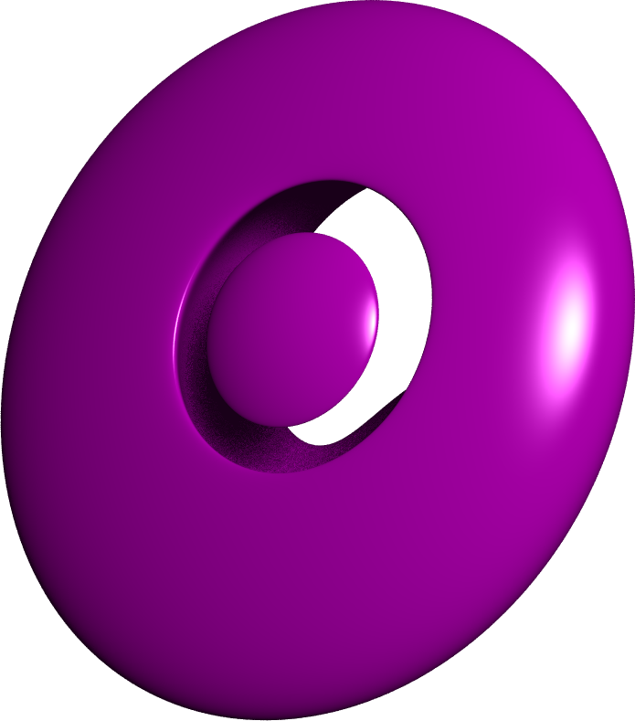
Figure 6. The front and the back view of a quartic smooth surface.

We implemented the algorithm in Maple and tested it on a computer with an Intel I7-5600 processor (1400 MHz). We report the timings in Table 1. The examples were surfaces of degree $4$ and $5$ with various types of singularities; the non-smooth cases are obtained by computing a random projection from a smooth model in a higher dimensional projective space. The coefficients used in these random constructions were $5$ decimal digit rational numbers chosen randomly. We projected the test surfaces to $\mathbb{P}^{2}$ and used Algorithm ReconstructGeneralSurface to reconstruct them. Some of these test surfaces were ruled, and in this case we developed another algorithm — which will be the subject of another paper — that proves to be faster than the one presented here if we know a point on the proper silhouette.

As for the choice of the pinch points in Step $2$, we took advantage of the fact that our surfaces were defined over $\mathbb{Q}$: we chose the conjugacy class of points whose cardinality coincides with the known number of pinch points.

Table 1. The table shows the degree of the surface $S$, of the proper silhouette $B$, and of the singular image $W$; then the number of nodes and cusps of $B$, the number of nodes and triple points of $W$, the number of tangential intersections, pinch points, and other transversal intersection points, and the computing time in CPU seconds.

$d$	$B$	$W$	$n(B)$	$c(B)$	$n(W)$	$t(W)$	$t$	$p$	$o$	time	type
4	8	2	8	12	1	0	0	8	4	12s	ruled (elliptic base)
4	8	2	4	12	0	0	4	4	4	6s	Del Pezzo
4	6	3	4	6	1	0	2	4	6	4s	ruled
4	12	0	12	24	0	0	0	0	0	5s	smooth
4	6	3	0	9	0	1	6	6	3	3s	Veronese
5	20	0	60	60	0	0	0	0	0	180s	smooth
5	10	5	12	18	3	1	18	8	12	400s	Del Pezzo
5	8	6	12	9	6	1	12	6	15	130s	ruled

Example 4.13 (Quartic Del Pezzo surface).

A general projection of a smooth quartic Del Pezzo surface in $\mathbb{P}^{4}$ to $\mathbb{P}^{3}$ is a quartic surface $S$. The singular curve $Z$ of $S$ is an irreducible conic.

The proper silhouette is an octic curve. To produce a concrete example, we start with the surface $S$ with the following equation:

$$(x^{2}+y^{2}-w^{2})^{2}-z^{2}(x^{2}-y^{2})+z^{4}=0\,.$$

The singular locus $Z$ is given by the conic

$$z=x^{2}+y^{2}-w^{2}=0\,.$$

By projecting from the point $\left(\frac{2987}{918}:\frac{58}{33}:\frac{29}{6}:1\right)$, the singular locus is mapped isomorphically to the plane conic $W$ with equation $x^{2}+y^{2}-w^{2}=0$. The proper silhouette $B$ is an octic with 2 real components. The curves $B$ and $W$ intersect in 4 points tangentially and in 8 points transversally. Four of them are images of pinch points. We see only two of the remaining $4$ because the other two are not real.

If we specify the correct pinch points, then the reconstruction algorithm returns the surface $S$. If we specify the other four points as pinch points, then we obtain another surface $S^{\prime}$ that has only two real pinch points (see Figure 7). Any other choice of pinch points does not give a surface.

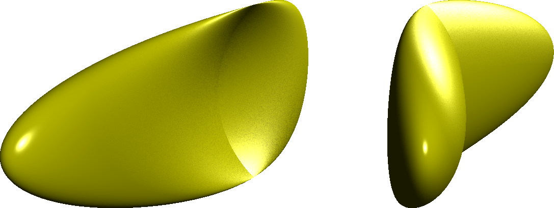
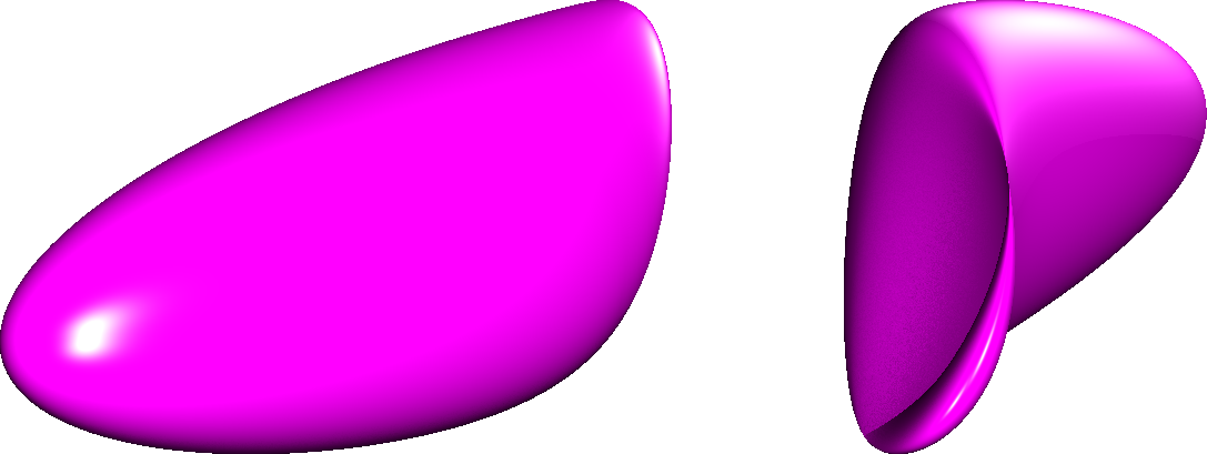
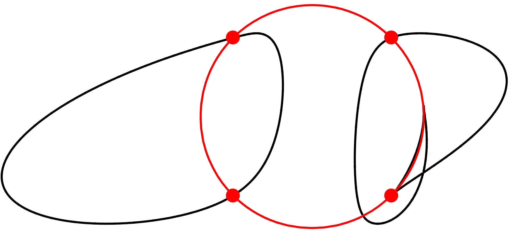
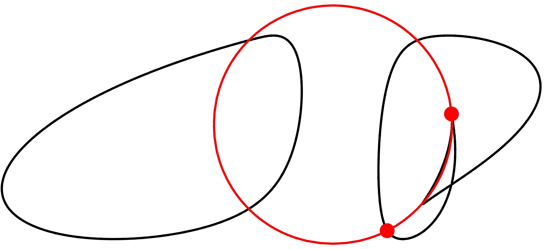
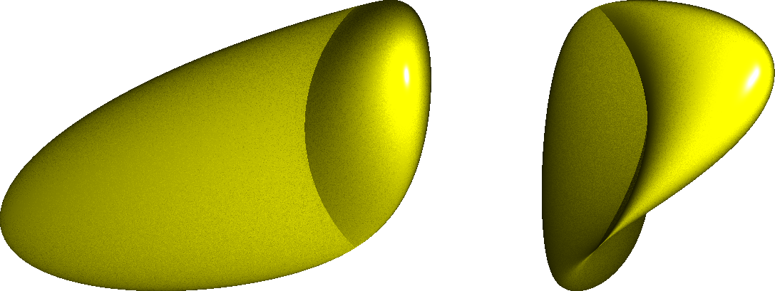
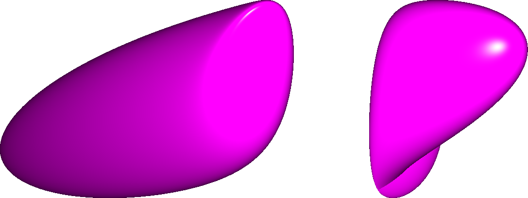
Figure 7. Two quartic surfaces with a singular conic with the same silhouette. The surface on the left, with front view, silhouette, and back view, has four real pinch points. The surface on the right has two real pinch points.

Remark 4.14.

If a quadratic equation of the singular curve $Z$ of a surface as in Example 4.13 is positive definite, then by a change of coordinates we can suppose that $Z$ is given by

$$w=x^{2}+y^{2}+z^{2}=0\,.$$

Hence we see that if we fix a positive definite quadratic equation of $Z$, we get a scalar product in the affine space $\mathbb{A}^{3}$ obtained by removing the plane carrying $Z$. This gives the space $\mathbb{A}^{3}$ the structure of a Euclidean space; the conic $Z$ is the absolute conic with respect to this structure (by definition, this is a conic without real points in the plane at infinity). The reason for this setup is that, despite $Z$ has no real points, it can still be “seen” in a photographic image obtained by central projection from a point $p\in\mathbb{A}^{3}$. The trick is to use a calibrated camera (see [17, Section 1.1]): if we mark the footpoint $q$ of $p$ on the image plane and the intersection of this plane with a right circular cone with vertex $p$ and axis through $q$ and angle $\frac{\pi}{4}$ (any other fixed angle would equally work), then all viewing angles $\sphericalangle(q_{1},p,q_{2})$ for $q_{1},q_{2}$ in the image plane can be computed by simple trigonometry. Hence the image plane is an elliptic plane, which means that we prescribe on it a conic without real points; in this case, this conic is the image of $Z$ under the projection.

In this case, the two surfaces $S_{1}$ and $S_{2}$ that are obtained by reconstruction are related by a spherical inversion with midpoint at the center of the projection. The reason for that is that the inversion of a quartic surface with the absolute conic as double curve is again a quartic surface with the absolute conic as double curve.

Example 4.15 (Veronese surface).

The general projection of a Veronese surface is a quartic surface $S$ with three singular lines $Z_{1},Z_{2},Z_{3}$ meeting in a triple point. Such a surface is called a Roman or Steiner surface, and is projectively equivalent to the surface of equation

$$x^{2}y^{2}+x^{2}z^{2}+y^{2}z^{2}+xyzw=0\,.$$

In this example, the three singular lines are the coordinate axes through the point $(0\colon 0\colon 0\colon 1)$. Each line contains two pinch points. The silhouette consists of three lines $W_{1},W_{2},W_{3}$ (the singular image) and a sextic $B$ with $9$ cusps (the proper silhouette). Each line $W_{i}$, for $i=1,2,3$, is tangent to $B$ at one point and intersects $B$ transversally in $4$ points. In order to recover the surface from the silhouette, we need to choose which are the projections of the $2$ pinch points on a line $Z_{i}$ among the four points of intersection between $W_{i}$ and $B$. There are $216$ possible cases.

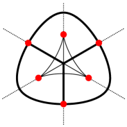
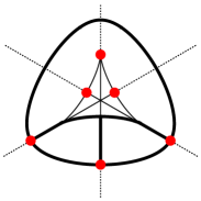
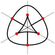
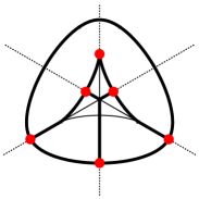
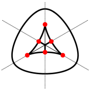
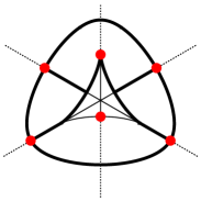
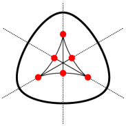
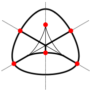
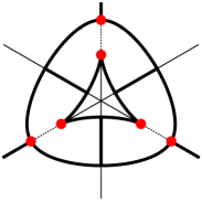
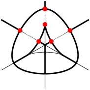
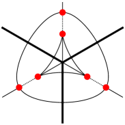
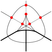
Figure 8. These diagrams show the hidden parts and isolated lines of six non-equivalent Roman surfaces projecting to the same silhouette, front and back view. Six others can be obtained by rotating the three surfaces on the right by $120^{\circ}$ and $240^{\circ}$. Diagrams in the same double row are obtained by factorizing the same projection from the Veronese surface to $\mathbb{P}^{2}$.

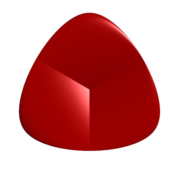
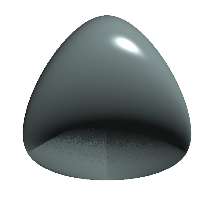
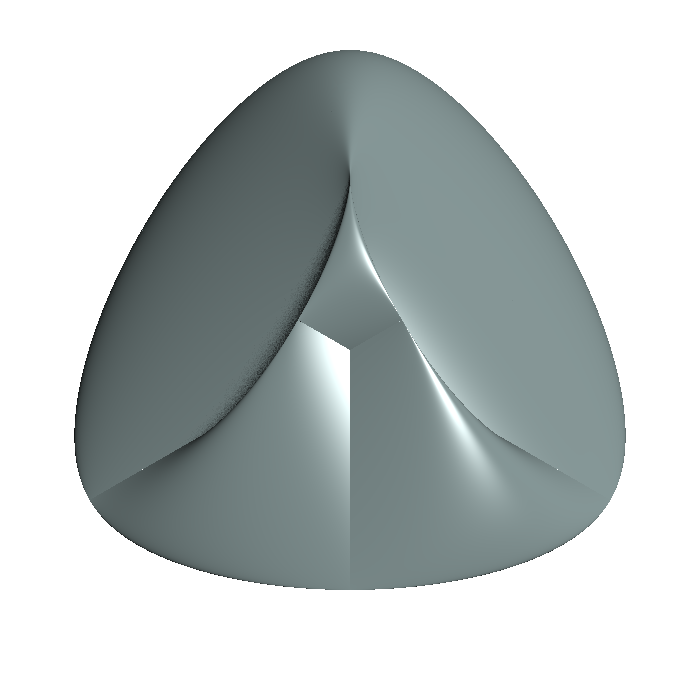
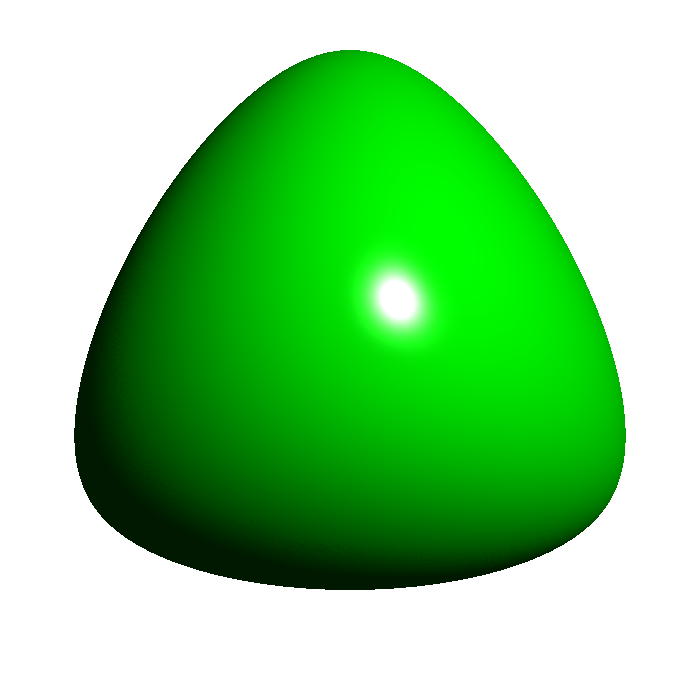
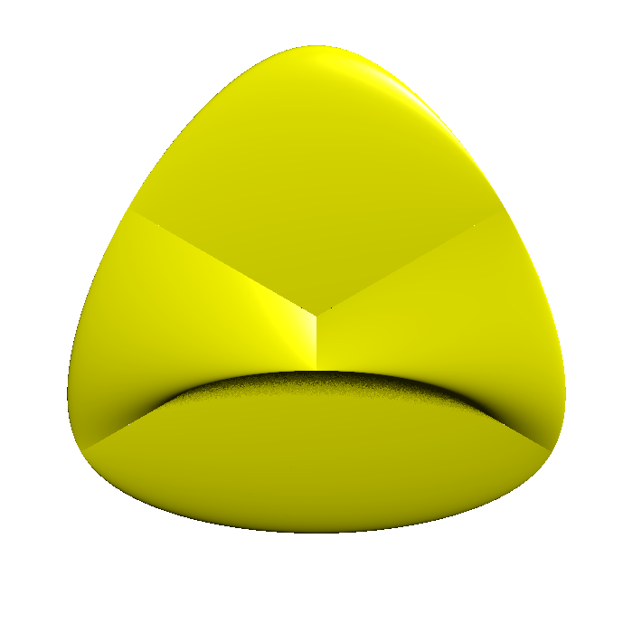
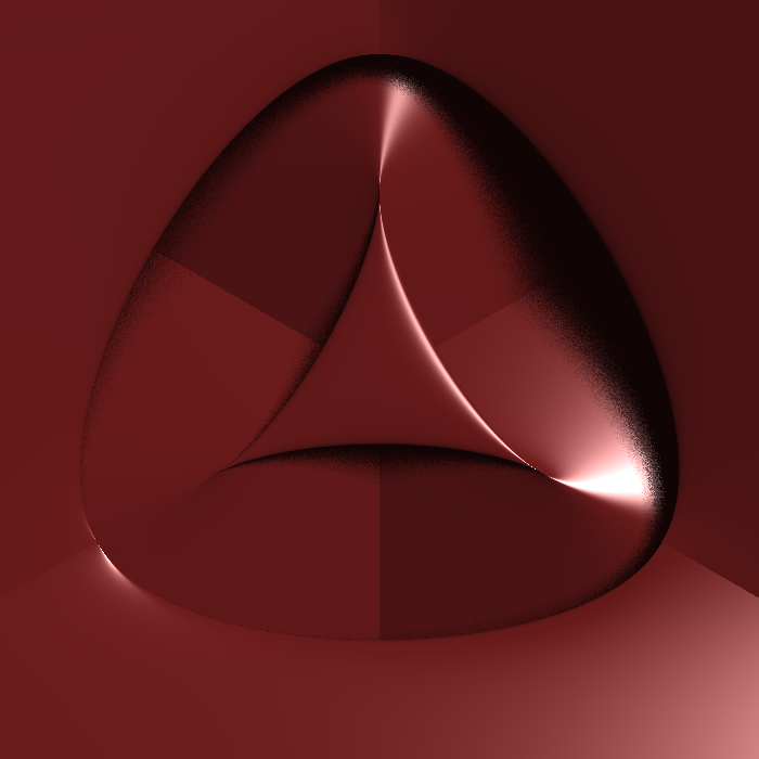
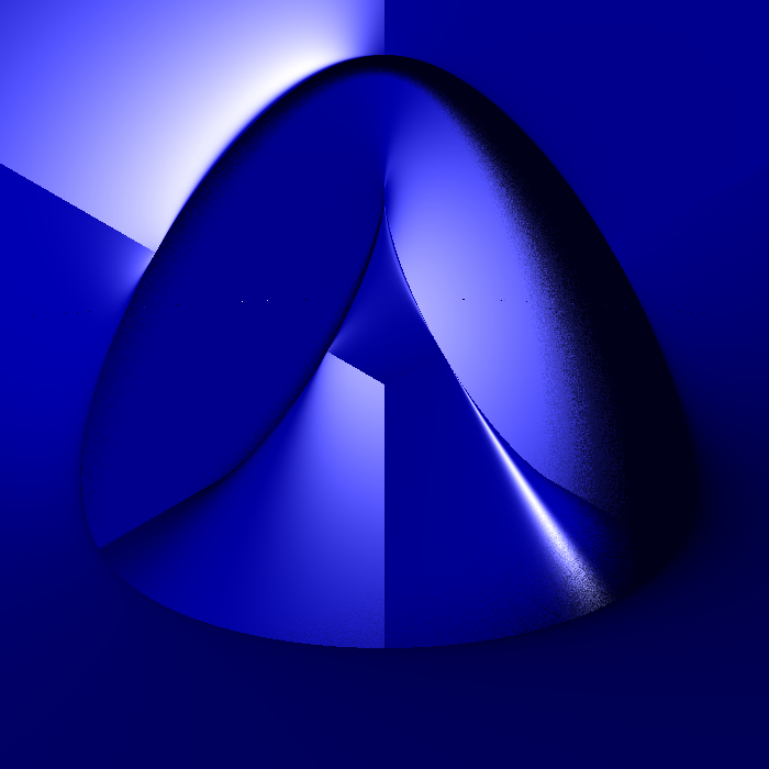
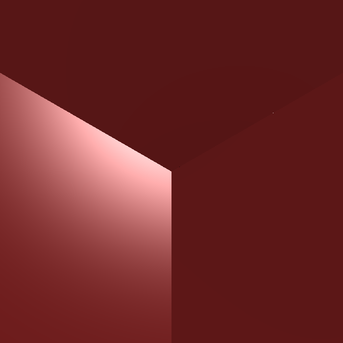
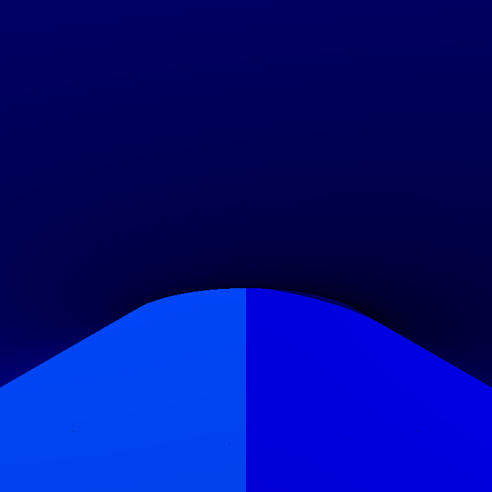
Figure 9. Here are six non-equivalent Roman surfaces with the same silhouette, front and back view, corresponding to the diagrams in Figure 8.

The computation using our algorithm shows that $204$ choices lead to an error message, while $12$ choices lead to a Roman surface. Let us say that two such surfaces $S_{1}$ and $S_{2}$, both coming with a projection $f_{i}\colon S_{i}\longrightarrow\mathbb{P}^{2}$, are Veronese-equivalent if there is a Veronese surface $V\in\mathbb{P}^{5}$ and projection maps $g_{i}\colon V\longrightarrow S_{i}$ such that $g_{1}\circ f_{1}=g_{2}\circ f_{2}$. Then the 12 Roman surfaces are partitioned into three Veronese-equivalence classes, each consisting of four surfaces. The fact that there are three different ways to project a Veronese surface to $\mathbb{P}^{2}$ for a fixed branching curve $B$ has been found by Catanese, see [6, Proposition 3.11], improving an example of Chisini. The four different choices of factoring each of these three maps through a Roman surface are explained by the fact that that the preimage of the intersection point of the three lines $W_{1},W_{2},W_{3}$ consists of $4$ points in the Veronese surface, and three of them are mapped to the triple point of the Roman surface: there are four ways to choose a triple out of four points.

In Figure 9, we show $6$ non-equivalent Roman surfaces with the same silhouette. They are divided in three groups, giving the three Veronese-equivalence classes. The diagrams in Figure 8 displays which parts of the silhouette are visible and which are hidden, and also which parts of the singular line are self-intersections and which are isolated lines. We see that for each Veronese-equivalence class we have an example where the visible/hidden structure is invariant under rotations by $\pi/3$, and another which is not. By applying rotations to the non-invariant example, we get two more non-equivalent surfaces that are in the same Veronese-equivalence class. In this way we get all the $12$ non-equivalent Roman surfaces.

For four surfaces in Figure 9, it is possible to find a hyperplane not intersecting the Roman surface, so we can display front and back view (see Remark 4.12). For the remaining two, we choose two hyperplanes at infinity that do not separate special points in order to produce front and back view.

Appendix A Computation of conductor ideals

The aim of this appendix is to explain how to compute the image of the map

$$\mathscr{H}\!\!om_{\mathscr{O}_{C}}\bigl{(}\pi_{\ast}\mathscr{O}_{Y},\mathscr{O}_{C}\bigr{)}_{c}\otimes\widehat{\mathscr{O}}_{C,c}\longrightarrow\widehat{\mathscr{O}}_{C,c}\,,$$

namely the conductor ideal, when $c\in C$ is a special point of the silhouette. We proceed by first determining normal forms for the projection around the special points, then computing the conductor ideals in those particular situations, and eventually finding equivariant formulas for these ideals that can hence be used without reducing the situation to normal forms.

We start by providing normal forms for each of the seven cases of singularities of the silhouette. Recall the notation from Lemma 4.8:

$$E=\widehat{\mathscr{O}}_{C,c}\quad\text{and}\quad F=\bigoplus_{y_{i}\colon\pi(y_{i})=c}\widehat{\mathscr{O}}_{Y,y_{i}}\,.$$

In each case we express the generators of $F$ as quotients of elements in $E$, as predicted by Lemma 4.8.

• Nodes of the proper silhouette. It is well-known that nodes are $A_{1}$ singularities, so they are analytically isomorphic to $\{(x,y)\in\mathbb{C}^{2}\,\colon\,xy=0\}$. Since the projection $\pi$ is an isomorphism away from the node, then the preimage of an analytic neighborhood of the node $c$ is constituted of two irreducible smooth curves, each of them isomorphic to the two components of $\{xy=0\}$. Hence they are analytically equivalent to two disjoint lines, and so we can suppose that

  $$E=\frac{\mathbb{C}[\![{x,y}]\!]}{(xy)}\quad\text{and}\quad F=\frac{\mathbb{C}[\![{x,y,z}]\!]}{\bigl{(}z(1-z),xz,y(1-z)\bigr{)}}\,,$$

  and the map $E\longrightarrow F$ is the natural inclusion sending the classes of $x$ and $y$ in $E$ to the classes of $x$ and $y$ in $F$. Since $F$ is generated, as an $E$-module, by the classes of $1$ and $z$, it is enough to show that $[z]$ can be expressed as a quotient of two elements $p,q\in E$, where $q$ is a non-zerodivisor. We have

  $$[z]=\frac{[z][x+y]}{[x+y]}=\frac{[y]}{[x+y]}$$

  and $[x+y]$ is not a zerodivisor in $E$.

• Cusps of the proper silhouette. It is well-known that ordinary cusps are $A_{2}$ singularities, so they are analytically isomorphic to $\{(x,y)\in\mathbb{C}^{2}\,\colon\,x^{3}-y^{2}=0\}$. The preimage under the projection $\pi$ of an analytic neighborhood of a cusp is a resolution of the cusp, so we can suppose

  $$E=\frac{\mathbb{C}[\![{x,y}]\!]}{(x^{3}-y^{2})}\quad\text{and}\quad F=\frac{\mathbb{C}[\![{x,y,z}]\!]}{(x-z^{2},y-z^{3},x^{3}-y^{2})}\,.$$

  Again, it is enough to express $[z]$ as the quotient of two elements in $E$, and indeed we have $[z]=[y]/[x]$.

• Nodes of the singular image. This case is similar to the one of the node of the proper silhouette, but we have to take into account that the fat silhouette has a non-reduced structure. The radical of the analytic ideal of node can be hence supposed to be $(xy)$, so the ideal is of the form $(x^{a}y^{b})$. As we saw at the end of the proof of Proposition 4.2, we have $a=b=2$. So

  $$E=\frac{\mathbb{C}[\![{x,y}]\!]}{(x^{2}y^{2})}\quad\text{and}\quad F=\frac{\mathbb{C}[\![{x,y,z}]\!]}{\bigl{(}z(1-z),x^{2}z,y^{2}(1-z)\bigr{)}}\,.$$

  We conclude as in the case of the nodes of the proper contour.

• Triple points of the singular image. A triple point of the singular image is the projection of a triple point of the surface. Such a point is analytically at the intersection of three smooth manifolds, each of which projects isomorphically to the plane. Hence, these manifolds are graphs of functions, so they are analytically equivalent to $\{(x,y,z)\in\mathbb{C}^{3}\,\colon\,z-f_{i}(x,y)=0\}$ for $i\in\{1,2,3\}$ and $f_{i}$ are analytic functions vanishing at $(0,0)$. By an analytic change of coordinates fixing the $(x,y)$-coordinates, we can assume $f_{1}=0$. The projection of the singular curve in the plane is the product $f_{2}f_{3}(f_{2}-f_{3})$. In the plane we have an ordinary triple point, so the tangents at $(0,0)$ to $\{f_{2}=0\}$ and $\{f_{3}=0\}$ are distinct, hence by the inverse function theorem we can suppose that $f_{2}=x$ and $f_{3}=y$. Therefore, we have

  $$E=\frac{\mathbb{C}[\![{x,y}]\!]}{\bigl{(}x^{2}y^{2}(x-y)^{2}\bigr{)}}\quad\text{and}\quad F=\frac{\mathbb{C}[\![{x,y,z}]\!]}{\bigl{(}z(z-x)(z-y),3z^{2}-2z(x+y)+xy\bigr{)}}\,,$$

  where the exponents are justified as in the previous case. In this case, $F$ is generated over $E$ by $[1]$, $[z]$ and $[z^{2}]$. The equation $3z^{2}-2z(x+y)+xy=0$ provides a linear dependence over $E$ between $[z]$ and $[z^{2}]$ that is monic in $[z^{2}]$, so it is enough to show that $[z]$ can be expressed as a quotients of elements in $E$. Taking division with remainder of $z(z-x)(z-y)$ by $3z^{2}-2z(x+y)+xy$ as polynomials in $z$, we get

  $$[z]=\frac{[x][y][x+y]}{2[x^{2}]+2[y^{2}]-2[xy]}\,.$$

• Transverse intersections of proper silhouette and singular image whose preimages are two distinct points. Here we have

  $$E=\frac{\mathbb{C}[\![{x,y}]\!]}{(xy^{2})}\quad\text{and}\quad F=\frac{\mathbb{C}[\![{x,y,z}]\!]}{\bigl{(}z(1-z),xz,y^{2}(1-z)\bigr{)}}\,,$$

  and so $[z]=[y^{2}]/([x]+[y^{2}])$.

• Transverse intersections of proper contour and singular images whose preimages are pinch points. We prove that the projection $\pi$ is an isomorphism in this situation, so we have $E=F$. Recall from Proposition 2.1 that we can assume that the local equation of the surface at a pinch point is $x^{2}y-z^{2}=0$ while keeping the projection along the $z$-axis. Its derivative with respect to $z$ is $2z$, so the fat contour is the plane curve $x^{2}y$ inside the plane $z=0$, thus the fat contour projects isomorphically to the fat silhouette.

• Tangential intersections of proper silhouette and singular image. Locally, the singular curve is the intersection of two smooth components $S_{1}$ and $S_{2}$ of the surface $S$, and one of the two, say $S_{1}$, contains the proper contour. The restriction of the projection to $S_{1}$ is a $2\colon 1$ covering branched along a smooth curve; we can choose analytic coordinates such that the equation of $S_{1}$ is $z^{2}-y=0$, the proper contour is $y=z=0$, and the proper silhouette is $y=0$. The second component $S_{2}$ projects isomorphically to the $xy$-plane, hence it has a local analytic equation of the form $z-f$, where $f$ is a function of $x$ and $y$. The two components of the silhouette are hence $y=0$ and $f^{2}-y=0$, obtained by eliminating $z$ from the previous equations. We know that the intersection multiplicity is $2$. This implies that the gradient of $f$ is independent from $y$. Hence we can choose $f=x$ as the third coordinate. In this coordinate system, we get

  $$E=\frac{\mathbb{C}[\![{x,y}]\!]}{\bigl{(}y(x^{2}-y)^{2}\bigr{)}}\quad\text{and}\quad F=\frac{\mathbb{C}[\![{x,y,z}]\!]}{\bigl{(}(z-x)(z^{2}-y),z^{2}-y+2z(z-x)\bigr{)}}\,.$$

  As in the case of triple points, the module $F$ is generated by $[1]$, $[z]$, and $[z^{2}]$. We get quotient representations for these elements in an analogous way (namely, by polynomial division):

  $$[z]=\frac{[4xy]}{[3y+x^{2}]}\,.$$

Lemma A.1.

For each of the seven types of special points of the fat silhouette $C$, the conductor ideals of the normal forms provided above are:

Type of singularity	Conductor ideal
Nodes of the proper silhouette	$\bigl{(}[x],[y]\bigr{)}$
Cusps of the proper silhouette	$\bigl{(}[x],[y]\bigr{)}$
Nodes of the singular image	$\bigl{(}[x^{2}],[y^{2}]\bigr{)}$
Triple points of the singular image	$\bigl{(}[x^{2}-xy+y^{2}],$
	$[xy(x+y)]\bigr{)}$
Transverse intersections of prop. silhouette and sing. image	$\bigl{(}[x],[y^{2}]\bigr{)}$
whose preimages are two distinct points
Transverse intersections of prop. silhouette and sing. image	$\bigl{(}[1]\bigr{)}$
whose preimages are pinch points
Tangential intersections of prop. silhouette and sing. image	$\bigl{(}[xy],[3y+x^{2}]\bigr{)}$

Proof.

We analyze each case separately.

• Nodes of the proper silhouette. Since $F$ is generated over $E$ by $[1]$ and $[z]$, the conductor ideal is $\{[\alpha]\in E\,\colon\,[\alpha z]\in E\}$. Hence we look for $[\alpha]\in E$ such that $[\alpha y]=[\beta(x+y)]$ for some $\beta\in\mathbb{C}[\![{x,y}]\!]$ (recall the description of $[z]$ as a quotient of elements of $E$). We calculate (in the standard polynomial ring, by means of computer algebra) the intersection of the two ideals $(y,xy)$ and $(x+y,xy)$, which is $(xy,y^{2})$. This implies that the conductor ideal is $([x],[y])$, because this equals the colon ideal $(xy,y^{2})\colon(y)$.

• Cusps of the proper silhouette. As in the previous case, it is enough to compute the intersection of the two ideals $(y,x^{3}-y^{2})$ and $(x,x^{3}-y^{2})$, which is $(y^{2},xy,x^{3})$. From this it follows that the conductor ideal is $([x],[y])$.

• Nodes of the singular image. This case is analogous to the one of nodes of the proper silhouette.

• Triple points of the singular image. This case is analogous to the one of nodes of the proper silhouette.

• Transverse intersections of proper silhouette and singular image whose preimages are two distinct points. This case is analogous to the one of nodes of the proper silhouette.

• Transverse intersections of proper contour and singular images whose preimages are pinch points. Since here $E=F$, the conductor is the trivial ideal.

• Tangential intersections of proper silhouette and singular image. This case is analogous to the one of nodes of the proper silhouette.

∎

One could think that Lemma A.1 provides a way to compute the conductor ideals of the special points from the knowledge of the fat silhouette: one could think, in fact, of bringing each of the special points to the corresponding normal form, and then pick the conductor ideal from the table. This would not be correct, since by knowing only the fat silhouette we do not have control on the fat contour, and so we cannot ensure that the preimages of the special points are in normal form. This seems a hindrance to the creation of an algorithm having as input only the fat silhouette, because the conductor ideal may depend on the fat contour. We now show that this is not the case.

Lemma A.2.

The conductor ideals at the special points depend only on the fat silhouette.

Proof.

We show that the ideals determined in Lemma A.1 for the normal forms are equivariant under analytic changes of coordinates in the plane, thus proving the statement.

• Nodes of the proper silhouette. In this case, the conductor ideal is just the maximal ideal of $\widehat{\mathscr{O}}_{C,c}$.

• Cusps of the proper silhouette. Same situation as for the nodes.

• Nodes of the singular image. Here the conductor ideal is the sum of the squares of the two ideals defining the two analytic components of the node.

• Triple points of the singular image. Let $f$ be an analytic local equation of the fat silhouette at a triple point. We then know that we can write $f=h_{1}h_{2}h_{3}$ with $h_{1}+h_{2}+h_{3}=0$ for some power series $\{h_{i}\}$ of order one. We prove that the conductor ideal equals

  $$J:=\bigl{(}a_{1}^{2}+a_{2}^{2}+a_{3}^{2}\,\colon\,a_{i}\in(h_{i})\text{ for }i\in\{1,2,3\}\text{ and }a_{1}+a_{2}+a_{3}=0\bigr{)}\,.$$

  Since the latter ideal has a formulation that is equivariant under analytic changes of coordinates, it is enough to check that $J$ coincides with the conductor ideal in the situation of the normal form, namely when

  $$h_{1}=-x,\quad h_{2}=y,\quad h_{3}=x-y\,.$$

  Recall that in this case the conductor ideal is $I=(x^{2}-xy+y^{2},x^{2}y+xy^{2})$. We first show the containment $J\subset I$. Consider an element in $J$, namely pick

  $$a_{1}=-\alpha x,\quad a_{2}=\beta y,\quad a_{3}=\gamma(x-y)=\alpha x-\beta y\,.$$

  for some $\alpha,\beta,\gamma\in\mathbb{C}[\![{x,y}]\!]$. This forces $\alpha=\gamma-uy$ and $\beta=\gamma+ux$ for some $u\in\mathbb{C}[\![{x,y}]\!]$. A direct computation shows that

  $$a_{1}^{2}+a_{2}^{2}+a_{3}^{2}=2\gamma^{2}(x^{2}-xy+y^{2})+2\gamma u(x^{2}y+xy^{2})+2u^{2}x^{2}y^{2}$$

  and hence $a_{1}^{2}+a_{2}^{2}+a_{3}^{2}\in I$, since one can check that $I$ contains $(x,y)^{4}$. To prove the opposite inclusion, it is enough to show that $x^{2}-xy+y^{2}$ and $x^{2}y+xy^{2}$ are in $J$. The first case is immediate, since $2(x^{2}-xy+y^{2})=(-x)^{2}+y^{2}+(x-y)^{2}$. For the second element, it is enough to pick the two triples $(a_{1},a_{2},a_{3})$ corresponding to $(\gamma,u)=(1,1)$ and to $(\gamma,u)=(1,-1)$, and to subtract the corresponding sums of squares.

• Transverse intersections of proper silhouette and singular image whose preimages are two distinct points. Here the conductor ideal is the sum of the ideal of the proper silhouette and of the square of the ideal of the singular image.

• Transverse intersections of proper contour and singular images whose preimages are pinch points. In this case the conductor is the trivial ideal.

• Tangential intersections of proper silhouette and singular image. As we did in the case of triple points of the singular image, we provide an equivariant description of the conductor ideal. Consider the situation of the normal form, where the conductor ideal is $I=(xy,3y+x^{2})$. Notice that it equals the ideal

  $$J:=\bigl{\{}a\in\mathbb{C}[\![{x,y}]\!]\,\colon\,a(0,0)=0\text{ and }\operatorname{mult}_{(0,0)}(a,3y+x^{2})\geq 3\bigr{\}}\,.$$

  We show that the latter description is equivariant under changes of analytic coordinates. Consider the following setting (see Figure 10): pick an analytic neighborhood of a tangential intersection of proper silhouette and singular image, and apply to it an analytic isomorphism. Blow up the two analytic neighborhoods at the tangential intersection; the previous analytic isomorphism then extends to an isomorphism of two neighborhoods of the exceptional divisors, which restricts to an automorphism of $\mathbb{P}^{1}$ on the exceptional divisors. After the blow up, the strict transforms of proper silhouette and singular image intersect transversally, and the exceptional divisor passes through that point of intersection. A further blow up separates these three curves and introduces a second exceptional divisor intersecting each of them transversally.

  \begin{overpic}[width=433.62pt]{pictures/tangential_invariant_dots.jpg} \put(39.0,10.0){$\lx@xy@svg{\hbox{\raise 0.0pt\hbox{\kern 3.0pt\hbox{\ignorespaces\ignorespaces\ignorespaces\hbox{\vtop{\kern 0.0pt\offinterlineskip\halign{\entry@#!@&&\entry@@#!@\cr&\crcr}}}\ignorespaces{\hbox{\kern-3.0pt\raise 0.0pt\hbox{\hbox{\kern 0.0pt\raise 0.0pt\hbox{\hbox{\kern 3.0pt\raise 0.0pt\hbox{$\textstyle{\ignorespaces\ignorespaces\ignorespaces\ignorespaces}$}}}}}}}\ignorespaces\ignorespaces\ignorespaces\ignorespaces{}{\hbox{\lx@xy@droprule}}\ignorespaces\ignorespaces\ignorespaces{\hbox{\kern 11.60136pt\raise 6.15pt\hbox{{}\hbox{\kern 0.0pt\raise 0.0pt\hbox{\hbox{\kern 3.0pt\hbox{\hbox{\kern 0.0pt\raise-1.75pt\hbox{$\scriptstyle{\cong}$}}}\kern 3.0pt}}}}}}\ignorespaces{\hbox{\kern 31.45274pt\raise 0.0pt\hbox{\hbox{\kern 0.0pt\raise 0.0pt\hbox{\lx@xy@tip{1}\lx@xy@tip{-1}}}}}}{\hbox{\lx@xy@droprule}}{\hbox{\lx@xy@droprule}}{\hbox{\kern 31.45274pt\raise 0.0pt\hbox{\hbox{\kern 0.0pt\raise 0.0pt\hbox{\hbox{\kern 3.0pt\raise 0.0pt\hbox{$\textstyle{}$}}}}}}}\ignorespaces}}}}\ignorespaces$} \put(39.0,42.0){$\lx@xy@svg{\hbox{\raise 0.0pt\hbox{\kern 3.0pt\hbox{\ignorespaces\ignorespaces\ignorespaces\hbox{\vtop{\kern 0.0pt\offinterlineskip\halign{\entry@#!@&&\entry@@#!@\cr&\crcr}}}\ignorespaces{\hbox{\kern-3.0pt\raise 0.0pt\hbox{\hbox{\kern 0.0pt\raise 0.0pt\hbox{\hbox{\kern 3.0pt\raise 0.0pt\hbox{$\textstyle{\ignorespaces\ignorespaces\ignorespaces\ignorespaces}$}}}}}}}\ignorespaces\ignorespaces\ignorespaces\ignorespaces{}{\hbox{\lx@xy@droprule}}\ignorespaces\ignorespaces\ignorespaces{\hbox{\kern 11.60136pt\raise 6.15pt\hbox{{}\hbox{\kern 0.0pt\raise 0.0pt\hbox{\hbox{\kern 3.0pt\hbox{\hbox{\kern 0.0pt\raise-1.75pt\hbox{$\scriptstyle{\cong}$}}}\kern 3.0pt}}}}}}\ignorespaces{\hbox{\kern 31.45274pt\raise 0.0pt\hbox{\hbox{\kern 0.0pt\raise 0.0pt\hbox{\lx@xy@tip{1}\lx@xy@tip{-1}}}}}}{\hbox{\lx@xy@droprule}}{\hbox{\lx@xy@droprule}}{\hbox{\kern 31.45274pt\raise 0.0pt\hbox{\hbox{\kern 0.0pt\raise 0.0pt\hbox{\hbox{\kern 3.0pt\raise 0.0pt\hbox{$\textstyle{}$}}}}}}}\ignorespaces}}}}\ignorespaces$} \put(39.0,82.0){$\lx@xy@svg{\hbox{\raise 0.0pt\hbox{\kern 3.0pt\hbox{\ignorespaces\ignorespaces\ignorespaces\hbox{\vtop{\kern 0.0pt\offinterlineskip\halign{\entry@#!@&&\entry@@#!@\cr&\crcr}}}\ignorespaces{\hbox{\kern-3.0pt\raise 0.0pt\hbox{\hbox{\kern 0.0pt\raise 0.0pt\hbox{\hbox{\kern 3.0pt\raise 0.0pt\hbox{$\textstyle{\ignorespaces\ignorespaces\ignorespaces\ignorespaces}$}}}}}}}\ignorespaces\ignorespaces\ignorespaces\ignorespaces{}{\hbox{\lx@xy@droprule}}\ignorespaces\ignorespaces\ignorespaces{\hbox{\kern 11.60136pt\raise 6.15pt\hbox{{}\hbox{\kern 0.0pt\raise 0.0pt\hbox{\hbox{\kern 3.0pt\hbox{\hbox{\kern 0.0pt\raise-1.75pt\hbox{$\scriptstyle{\cong}$}}}\kern 3.0pt}}}}}}\ignorespaces{\hbox{\kern 31.45274pt\raise 0.0pt\hbox{\hbox{\kern 0.0pt\raise 0.0pt\hbox{\lx@xy@tip{1}\lx@xy@tip{-1}}}}}}{\hbox{\lx@xy@droprule}}{\hbox{\lx@xy@droprule}}{\hbox{\kern 31.45274pt\raise 0.0pt\hbox{\hbox{\kern 0.0pt\raise 0.0pt\hbox{\hbox{\kern 3.0pt\raise 0.0pt\hbox{$\textstyle{}$}}}}}}}\ignorespaces}}}}\ignorespaces$} \put(18.0,30.0){$\lx@xy@svg{\hbox{\raise 0.0pt\hbox{\kern 3.0pt\hbox{\ignorespaces\ignorespaces\ignorespaces\hbox{\vtop{\kern 0.0pt\offinterlineskip\halign{\entry@#!@&&\entry@@#!@\cr\\\crcr}}}\ignorespaces{\hbox{\kern-3.0pt\raise 0.0pt\hbox{\hbox{\kern 0.0pt\raise 0.0pt\hbox{\hbox{\kern 3.0pt\raise 0.0pt\hbox{$\textstyle{\mbox{}\ignorespaces\ignorespaces\ignorespaces\ignorespaces}$}}}}}}}\ignorespaces\ignorespaces\ignorespaces\ignorespaces{}{\hbox{\lx@xy@droprule}}\ignorespaces\ignorespaces\ignorespaces{\hbox{\kern 0.0pt\raise-24.33955pt\hbox{{}\hbox{\kern 0.0pt\raise 0.0pt\hbox{\hbox{\kern 3.0pt\hbox{\hbox{\kern 0.0pt\raise-0.8264pt\hbox{$\scriptstyle{p_{1}}$}}}\kern 3.0pt}}}}}}\ignorespaces{\hbox{\kern 0.0pt\raise-45.67912pt\hbox{\hbox{\kern 0.0pt\raise 0.0pt\hbox{\lx@xy@tip{1}\lx@xy@tip{-1}}}}}}{\hbox{\lx@xy@droprule}}{\hbox{\lx@xy@droprule}}{\hbox{\kern-3.0pt\raise-48.67912pt\hbox{\hbox{\kern 0.0pt\raise 0.0pt\hbox{\hbox{\kern 3.0pt\raise 0.0pt\hbox{$\textstyle{\mbox{}}$}}}}}}}\ignorespaces}}}}\ignorespaces$} \put(18.0,68.0){$\lx@xy@svg{\hbox{\raise 0.0pt\hbox{\kern 3.0pt\hbox{\ignorespaces\ignorespaces\ignorespaces\hbox{\vtop{\kern 0.0pt\offinterlineskip\halign{\entry@#!@&&\entry@@#!@\cr\\\crcr}}}\ignorespaces{\hbox{\kern-3.0pt\raise 0.0pt\hbox{\hbox{\kern 0.0pt\raise 0.0pt\hbox{\hbox{\kern 3.0pt\raise 0.0pt\hbox{$\textstyle{\mbox{}\ignorespaces\ignorespaces\ignorespaces\ignorespaces}$}}}}}}}\ignorespaces\ignorespaces\ignorespaces\ignorespaces{}{\hbox{\lx@xy@droprule}}\ignorespaces\ignorespaces\ignorespaces{\hbox{\kern 0.0pt\raise-24.33955pt\hbox{{}\hbox{\kern 0.0pt\raise 0.0pt\hbox{\hbox{\kern 3.0pt\hbox{\hbox{\kern 0.0pt\raise-0.8264pt\hbox{$\scriptstyle{p_{2}}$}}}\kern 3.0pt}}}}}}\ignorespaces{\hbox{\kern 0.0pt\raise-45.67912pt\hbox{\hbox{\kern 0.0pt\raise 0.0pt\hbox{\lx@xy@tip{1}\lx@xy@tip{-1}}}}}}{\hbox{\lx@xy@droprule}}{\hbox{\lx@xy@droprule}}{\hbox{\kern-3.0pt\raise-48.67912pt\hbox{\hbox{\kern 0.0pt\raise 0.0pt\hbox{\hbox{\kern 3.0pt\raise 0.0pt\hbox{$\textstyle{\mbox{}}$}}}}}}}\ignorespaces}}}}\ignorespaces$} \put(68.0,30.0){$\lx@xy@svg{\hbox{\raise 0.0pt\hbox{\kern 3.0pt\hbox{\ignorespaces\ignorespaces\ignorespaces\hbox{\vtop{\kern 0.0pt\offinterlineskip\halign{\entry@#!@&&\entry@@#!@\cr\\\crcr}}}\ignorespaces{\hbox{\kern-3.0pt\raise 0.0pt\hbox{\hbox{\kern 0.0pt\raise 0.0pt\hbox{\hbox{\kern 3.0pt\raise 0.0pt\hbox{$\textstyle{\mbox{}\ignorespaces\ignorespaces\ignorespaces\ignorespaces}$}}}}}}}\ignorespaces\ignorespaces\ignorespaces\ignorespaces{}{\hbox{\lx@xy@droprule}}\ignorespaces\ignorespaces\ignorespaces{\hbox{\kern 0.0pt\raise-24.33955pt\hbox{{}\hbox{\kern 0.0pt\raise 0.0pt\hbox{\hbox{\kern 3.0pt\hbox{\hbox{\kern 0.0pt\raise-2.96667pt\hbox{$\scriptstyle{\widehat{p}_{1}}$}}}\kern 3.0pt}}}}}}\ignorespaces{\hbox{\kern 0.0pt\raise-45.67912pt\hbox{\hbox{\kern 0.0pt\raise 0.0pt\hbox{\lx@xy@tip{1}\lx@xy@tip{-1}}}}}}{\hbox{\lx@xy@droprule}}{\hbox{\lx@xy@droprule}}{\hbox{\kern-3.0pt\raise-48.67912pt\hbox{\hbox{\kern 0.0pt\raise 0.0pt\hbox{\hbox{\kern 3.0pt\raise 0.0pt\hbox{$\textstyle{\mbox{}}$}}}}}}}\ignorespaces}}}}\ignorespaces$} \put(68.0,68.0){$\lx@xy@svg{\hbox{\raise 0.0pt\hbox{\kern 3.0pt\hbox{\ignorespaces\ignorespaces\ignorespaces\hbox{\vtop{\kern 0.0pt\offinterlineskip\halign{\entry@#!@&&\entry@@#!@\cr\\\crcr}}}\ignorespaces{\hbox{\kern-3.0pt\raise 0.0pt\hbox{\hbox{\kern 0.0pt\raise 0.0pt\hbox{\hbox{\kern 3.0pt\raise 0.0pt\hbox{$\textstyle{\mbox{}\ignorespaces\ignorespaces\ignorespaces\ignorespaces}$}}}}}}}\ignorespaces\ignorespaces\ignorespaces\ignorespaces{}{\hbox{\lx@xy@droprule}}\ignorespaces\ignorespaces\ignorespaces{\hbox{\kern 0.0pt\raise-24.33955pt\hbox{{}\hbox{\kern 0.0pt\raise 0.0pt\hbox{\hbox{\kern 3.0pt\hbox{\hbox{\kern 0.0pt\raise-2.96667pt\hbox{$\scriptstyle{\widehat{p}_{2}}$}}}\kern 3.0pt}}}}}}\ignorespaces{\hbox{\kern 0.0pt\raise-45.67912pt\hbox{\hbox{\kern 0.0pt\raise 0.0pt\hbox{\lx@xy@tip{1}\lx@xy@tip{-1}}}}}}{\hbox{\lx@xy@droprule}}{\hbox{\lx@xy@droprule}}{\hbox{\kern-3.0pt\raise-48.67912pt\hbox{\hbox{\kern 0.0pt\raise 0.0pt\hbox{\hbox{\kern 3.0pt\raise 0.0pt\hbox{$\textstyle{\mbox{}}$}}}}}}}\ignorespaces}}}}\ignorespaces$} \put(16.0,6.0){$P$} \put(16.0,38.0){$Q$} \put(17.0,95.0){$R$} \put(4.0,44.0){$E_{1}$} \put(4.0,84.0){$E_{1}^{\prime}$} \put(21.0,72.0){$E_{2}$} \put(26.0,13.0){$B$} \put(26.0,4.0){$W$} \put(32.0,48.0){$B^{\prime}$} \put(32.0,36.0){$W^{\prime}$} \put(32.0,88.0){$B^{\prime\prime}$} \put(32.0,79.0){$W^{\prime\prime}$} \put(69.0,6.0){$\widehat{P}$} \put(69.0,38.0){$\widehat{Q}$} \put(69.0,95.0){$\widehat{R}$} \put(82.0,44.0){$\widehat{E}_{1}$} \put(82.0,84.0){$\widehat{E}^{\prime}_{1}$} \put(64.0,72.0){$\widehat{E}_{2}$} \put(60.0,13.0){$\widehat{B}$} \put(60.0,4.0){$\widehat{W}$} \put(53.0,48.0){$\widehat{B}^{\prime}$} \put(53.0,36.0){$\widehat{W}^{\prime}$} \put(53.0,88.0){$\widehat{B}^{\prime\prime}$} \put(53.0,79.0){$\widehat{W}^{\prime\prime}$} \end{overpic}

  Figure 10. Schematic view of the construction used to prove independence of the conductor ideal from the fat contour in the case of tangent intersections: we blow up the two curves $B$ and $W$ at their intersection $P$, obtaining an exceptional divisor $E_{1}$, which intersects the strict transforms $B^{\prime}$ and $W^{\prime}$ in a point $Q$. Blowing up again we introduce another exceptional divisor $E_{2}$. The conductor ideal can be interpreted as the ideal of functions vanishing at $P$, whose controlled transforms vanish at $Q$ and at a point $R$ of $E_{2}$. If we have an analytic isomorphism around the tangent intersection, the fact that it extends to an isomorphism on exceptional divisors proves that the image of $R$ is prescribed, since the isomorphism $E_{2}\longrightarrow\widehat{E}_{2}$ is an automorphism of $\mathbb{P}^{1}$ which must preserve the intersections of $E_{2}$ with the strict transforms $E_{1}^{\prime}$, $B^{\prime\prime}$ and $W^{\prime\prime}$.

  Let us use the following notation: we denote by $p_{1}$ the first blow up map, by $E_{1}$ its exceptional divisor, by $B^{\prime}$ and $W^{\prime}$ the strict transforms of $B$ and $W$; we denote by $p_{2}$ the second blow up map, by $E_{2}$ its exceptional divisor, and by $E_{1}^{\prime}$, $B^{\prime\prime}$ and $W^{\prime\prime}$ the strict transforms of $E_{1}$, $B^{\prime}$ and $W^{\prime\prime}$. Let $P$ be the tangential intersection of $B$ and $W$, let $Q$ be the intersection of $B^{\prime}$, $W^{\prime}$ and $E_{1}$. We show that the ideal $J$ coincides with

  $$K:=\bigl{\{}a\in\mathbb{C}[\![{x,y}]\!]\,\colon\,a(P)=0,\,p_{1}^{!}(a)(Q)=0,\,(p_{2}\circ p_{1})^{!}(a)(R)=0\bigr{\}}\,,$$

  where $p_{1}^{!}(a)$ is the controlled transform of $a$ under the blow up map $p_{1}$, and $R$ is a point on $E_{2}$. To show this, notice that $I$ is analytically equivalent to the ideal $(x^{3},y)$, and so $J$ can be described as the ideal of functions $a$ that vanish at $(0,0)$ and such that $\operatorname{mult}_{(0,0)}(a,y)\geq 3$, namely that are of the form $a=\sum_{i,j}a_{ij}x^{i}y^{j}$ with $i\geq 3$ or $j\geq 1$. Let us compute $K$ in this new setting: the condition $a(P)=0$ implies that if $a=\sum_{i,j}a_{ij}x^{i}y^{j}$, then $i\geq 1$ or $j\geq 1$. The controlled transform $p_{1}^{!}(a)$ equals, in the chart with coordinates $(x,\widetilde{y})$ with $y=\widetilde{y}x$, the function $\sum_{i,j}a_{ij}x^{i+j-1}\widetilde{y}^{j}$ — we subtract $1$ in the exponent of $x$ since in these coordinates $p_{1}^{!}(a)=p_{1}^{\ast}(a)/x$ because $x=0$ is the equation of the exceptional divisor; so, the condition $p_{1}^{!}(a)(Q)=0$ translates into $i+j-1\geq 1$ or $j\geq 1$. Similarly, the condition $(p_{2}\circ p_{1})^{!}(a)(R)=0$ translates to $i+2j-2\geq 1$ or $j\geq 1$. One can check that the conjunction of these three conditions is equivalent to the condition defining $J$. Hence the conductor ideal $I$ equals $K$, and we see that the description of $K$ is equivariant under local analytic changes of coordinates, because, as already mentioned, any such change extends to an isomorphism at the level of the exceptional divisors $E_{2}$, which are projective lines; since this isomorphism must preserve the intersections of $E_{2}$ with $E_{1}^{\prime}$, $B^{\prime\prime}$ and $W^{\prime\prime}$, it is uniquely determined, and so the same holds for the image of $R$ under it. This proves that the formation of the conductor ideal is equivariant.

∎

We conclude this appendix providing formulas to compute the conductor ideals of special points without the need of bringing the equation of the fat silhouette to a normal form. The proof of Lemma A.2 clarifies how to do so in the case of nodes and cusps of the proper silhouette, and of transversal intersections of proper silhouette and singular image (coming both from pinch points or pairs of distinct points). We are hence left with:

Nodes of the singular image:

If $f$ is a local analytic equation of the silhouette, namely of the reduced structure of the fat silhouette, one sees that the conductor ideal in the normal form is generated by the $2\times 2$ minors of the matrix

$$\begin{pmatrix}\partial_{xx}f&\partial_{xy}f&\partial_{yy}f&\partial_{x}f&\partial_{y}f\\ \partial_{xx}(f^{2})&\partial_{xy}(f^{2})&\partial_{yy}(f^{2})&\partial_{x}(f^{2})&\partial_{y}(f^{2})\end{pmatrix}\,.$$

We show that these formulas are equivariant under analytic changes of coordinates, and so they can be used for any node of the singular image. First of all, notice that the conductor ideal for the normal form contains the ideal $(x,y)^{3}$. This means that the conductor ideal always contains the third power of the maximal ideal of the point. Hence, in order to prove that the formulas we give are equivariant, it is enough to consider their part of order at most two. Locally analytically, the function $f$, which is of order two at the node, splits as a product $f=h_{1}h_{2}$, where each $h_{i}$ has order one. We show that any perturbation of the $h_{i}$ by an element of order at least two does not influence the equivariance property. In fact, suppose that we write $h_{1}=\widetilde{h}_{1}+\varepsilon$, where $\widetilde{h}_{1}$ has order one and $\varepsilon$ has order two. Then $f=\widetilde{h}_{1}h_{2}+\varepsilon h_{2}$, and so $\varepsilon h_{2}$ has order three. This means that any of the second derivatives of $f$ will be affected by a perturbation of order one. With similar computations, one sees that the second derivatives of $f^{2}$ are affected by a perturbation of order two. This implies that any minor of the previous matrix is affected by a perturbation of order at least three, which can be ignored since the conductor ideal contains the whole third power of the maximal ideal. Hence, in order to prove equivariance, it suffices to check that the formula we propose is equivariant under all coordinate changes of the form

$$\begin{pmatrix}x\\ y\end{pmatrix}\mapsto\begin{pmatrix}a_{1}\,x+a_{2}\,y\\ a_{3}\,x+a_{4}\,y\end{pmatrix}\,,$$

namely that it always provides the conductor ideal, which is given by $(h_{1}^{2},h_{2}^{2})$. These checks can performed for symbolic parameters $a_{1},\dotsc,a_{4}$ with the help of a computer algebra system. We implemented these tests in a Maple script inside the package we developed, see the introduction for the Internet address where to find the code.

Triple points of the singular image:

If $f$ is a local analytic equation for the silhouette, then one can check that the conductor ideal in the normal form is generated by the $2\times 2$ minors of the matrix

$$\begin{pmatrix}\partial_{xxx}f&\partial_{xxy}f&\partial_{xyy}f&\partial_{yyy}f\\ \partial_{xxx}(f^{2})&\partial_{xxy}(f^{2})&\partial_{xyy}(f^{2})&\partial_{yyy}(f^{2})\end{pmatrix}$$

together with

$$3\,f\,f_{xxx}\,f_{xyy}\,f_{xyyy}-3\,f\,f_{xxy}^{2}f_{xyyy}-3\,f\,f_{xxx}\,f_{yyy}\,f_{xxyy}+3\,f\,f_{xxy}\,f_{xyy}\,f_{xxyy}+$$

$$3\,f\,f_{xxy}\,f_{yyy}\,f_{xxxy}-3\,f\,f_{xyy}^{2}\,f_{xxxy}+2\,f_{xx}\,f_{xy}\,f_{xxy}\,f_{yyy}-2\,f_{xx}\,f_{xy}\,f_{xyy}^{2}+$$

$$2\,f_{xx}\,f_{yy}\,f_{xxx}\,f_{yyy}-2\,f_{xx}\,f_{yy}\,f_{xxy}\,f_{xyy}-4\,f_{xy}^{2}\,f_{xxx}\,f_{yyy}+4\,f_{xy}^{2}\,f_{xxy}\,f_{xyy}+$$

$$2\,f_{xy}\,f_{yy}\,f_{xxx}\,f_{xyy}-2\,f_{xy}\,f_{yy}\,f_{xxy}^{2}\,.$$

The last element has been computed by imposing that a symbolic linear combination of a list of candidates is in the conductor ideal for several randomized examples. As for the case of nodes, we show that these formulas are equivariant under analytic changes of coordinates. Since the conductor ideal of the normal form contains the ideal $(x,y)^{4}$, the conductor ideal always contains the fourth power of the maximal ideal of the point, and so we can neglect contributions of order at least four in the formulas. We know that for a triple point we always have, locally analytically, the factorization $f=h_{1}h_{2}(h_{1}-h_{2})$, where each $h_{i}$ has order one. Similarly as before, a direct inspection of the formulas shows that a perturbation of order at least three of the $h_{i}$ determines a perturbation of order at least four in the formula. Thus it is sufficient to check that the formulas are equivariant under changes of coordinates of the form

$$\begin{pmatrix}x\\ y\end{pmatrix}\mapsto\begin{pmatrix}a_{1}\,x+a_{2}\,y+b_{1}\,x^{2}+b_{2}\,xy+b_{3}\,y^{2},\\ a_{3}\,x+a_{4}\,y+b_{4}\,x^{2}+b_{5}\,xy+b_{6}\,y^{2}\end{pmatrix}\,,$$

namely that they always provide the conductor ideal, which is given by

$$\bigl{(}h_{1}^{2}+h_{2}^{2}+(h_{1}-h_{2})^{2},\,h_{1}^{2}h_{2}+h_{1}h_{2}^{2}\bigr{)}\,.$$

This is checked symbolically with the aid of computer algebra.

Tangential intersections of proper silhouette and singular image:

In this case, if $f$ and $g$ are local analytic equations of the proper silhouette and of the singular image, the conductor ideal in the normal form is given by

$$\bigl{(}fg,\,4f\thinspace\partial_{y}g-g\thinspace\partial_{y}f,\,4f\thinspace\partial_{x}g-g\thinspace\partial_{x}f\bigr{)}\,.$$

The proof of equivariance follows as in the previous cases.

References

[1]Persistence of Vision Pty. Ltd.Williamstown, Victoria, Australia. http://www.povray.org/.
[2]G. Biggiogero, La caratterizzazione della curva di diramazione dei
piani tripli, ottenuta mediante sistemi di curve pluritangenti, Ist.
Lombardo Sci. Lett. Rend Cl. Sci. Mat. Nat., LXXX (1947), pp. 151–160.
s. .
[3]G. Biggiogero, Sulla caratterizzazione della curva di diramazione
dei piani quadrupli generali, Ist. Lombardo Sci. Lett. Rend Cl. Sci. Mat.
Nat., LXXX (1947), pp. 269–280.
s. .
[4]N. Bourbaki, Elements of mathematics. Commutative algebra,
Springer-Verlag, Berlin, 1998.
[5]E. Boyer and M.-O. Berger, 3D Surface Reconstruction Using
Occluding Contours, Int. J. Comput. Vis., 22 (1997), pp. 219–233,
https://doi.org/10.1023/A:1007978616082.
[7]F. Catanese, Differentiable and deformation type of algebraic
surfaces, real and symplectic structures, in Symplectic 4-manifolds and
algebraic surfaces, vol. 1938 of Lecture Notes in Math., Springer, Berlin,
2008, pp. 55–167, https://doi.org/10.1007/978-3-540-78279-7_2.
[8]O. Chisini, Sulla identità birazionale di due funzioni algebriche
di più variabili, dotate di una medesima varietà di diramazione, Ist.
Lombardo Sci. Lett. Rend Cl. Sci. Mat. Nat. (3), 77 (1944), pp. 339–356.
[9]O. Chisini and C. F. Manara, Sulla caratterizzazione delle curve di
diramazione dei piani tripli, Ann. Mat. Pura Appl., 25 (1946), pp. 255–265,
https://doi.org/10.1007/BF02418084.
[10]C. Ciliberto and F. Flamini, On the branch curve of a general
projection of a surface to a plane, Trans. Amer. Math. Soc., 363 (2011),
pp. 3457–3471, https://doi.org/10.1090/S0002-9947-2011-05401-2.
[12]F. Enriques, Sulla costruzione delle funzioni algebriche di due
variabili possedenti una data curva di diramazione, Annali di Matematica
Pura ed Applicata, 1 (1924), pp. 185–198,
https://doi.org/10.1007/BF02409919.
[13]O. Faugeras and Q.-T. Luong, The geometry of multiple images, MIT
Press, Cambridge, MA, 2001.
[14]S. Finashin and V. Kharlamov, Apparent contours of nonsingular real
cubic surfaces, Trans. Amer. Math. Soc., 367 (2015), pp. 7221–7289,
https://doi.org/10.1090/S0002-9947-2015-06286-2.
[15]D. A. Forsyth, Recognizing algebraic surfaces from their outlines,
in 1993 (4th) International Conference on Computer Vision, May 1993,
pp. 476–480, https://doi.org/10.1109/ICCV.1993.378177.
[17]R. Hartley and A. Zisserman, Multiple view geometry in computer
vision, Cambridge University Press, 2nd ed., 2004,
https://doi.org/10.1017/CBO9780511811685.
[18]R. Hartshorne, Algebraic geometry, vol. 52 of Graduate Texts in
Mathematics, Springer-Verlag, New York-Heidelberg, 1977.
[19]S. Holzer and O. Labs, surfex 0.90, tech. report, University
of Mainz, University of Saarbrücken, 2008.
www.surfex.AlgebraicSurface.net.
[20]M. Joswig, J. Kileel, B. Sturmfels, and A. Wagner, Rigid
multiview varieties., Int. J. Algebra Comput., 26 (2016), pp. 775–788,
https://doi.org/10.1142/S021819671650034X.
[21]F. Kahl and K. Åström, Motion estimation in image sequences
using the deformation of apparent contours, in Sixth International
Conference on Computer Vision (IEEE Cat. No.98CH36271), Jan 1998,
pp. 939–942, https://doi.org/10.1109/ICCV.1998.710829.
[22]K. Kang, J. P. Tarel, R. Fishman, and D. Cooper, A linear dual-space
approach to 3D surface reconstruction from occluding contours using
algebraic surfaces, in Proceedings Eighth IEEE International Conference on
Computer Vision. ICCV 2001, vol. 1, 2001, pp. 198–204,
https://doi.org/10.1109/ICCV.2001.937518.
[23]J. Kileel, Minimal problems for the calibrated trifocal variety,
SIAM J. Appl. Algebra Geom., 1 (2017), pp. 575–598,
https://doi.org/10.1137/16M1104482.
[24]K. Kohn, B. Sturmfels, and M. Trager, Changing views on curves and
surfaces, Acta Math. Vietnam., 43 (2018), pp. 1–29,
https://doi.org/10.1007/s40306-017-0240-1.
[27]S. Manfredini and R. Pignatelli, Chisini’s conjecture for curves
with singularities of type , Michigan Math. J., 50 (2002),
pp. 287–312, https://doi.org/10.1307/mmj/1028575735.
[28]E. Mezzetti and D. Portelli, A tour through some classical theorems
on algebraic surfaces, An. Ştiinţ. Univ. Ovidius Constanţa Ser.
Mat., 5 (1997), pp. 51–78.
[30]B. G. Moishezon, Stable branch curves and braid monodromies, in
Algebraic geometry (Chicago, Ill., 1980), vol. 862 of Lecture Notes in
Math., Springer, Berlin-New York, 1981, pp. 107–192.
[32]J. Ponce, D. Chelberg, and W. B. Mann, Invariant properties of
straight homogeneous generalized cylinders and their contours, IEEE
Transactions on Pattern Analysis and Machine Intelligence, 11 (1989),
pp. 951–966, https://doi.org/10.1109/34.35498.
[33]J. Ponce and M. Hebert, On image contours of projective shapes, in
European Conference on Computer Vision, 2014.
[34]J. Ponce, B. Sturmfels, and M. Trager, Congruences and
concurrent lines in multi-view geometry., Adv. Appl. Math., 88 (2017),
pp. 62–91, https://doi.org/10.1016/j.aam.2017.01.001.
[35]B. Segre, Sulla caratterizzazione delle curve di diramazione dei
piani multipli generali, Memor. Reale Acc. d’Italia, 1 (1930), pp. 5–31.
[37]M. Trager, M. Hebert, and J. Ponce, Consistency of silhouettes and
their duals, in IEEE Conference on Computer Vision and Pattern Recognition,
2016.
[38]F. L. Zak, Tangents and secants of algebraic varieties, vol. 127 of
Translations of Mathematical Monographs, American Mathematical Society, 1993.
[39]O. Zariski, On the problem of existence of algebraic functions of
two variables possessing a given branch curve, Amer. J. Math., 51 (1929),
pp. 305–328, https://doi.org/10.2307/2370712.
[40]M. Zerroug and R. Nevatia, Quasi-invariant properties and 3-D
shape recovery of non-straight, non-constant generalized cylinders, in
Proceedings of IEEE Conference on Computer Vision and Pattern Recognition,
Jun 1993, pp. 96–103, https://doi.org/10.1109/CVPR.1993.340973.