Towards a correct and efficient implementation of simulation and verification tools for probabilistic ntcc

Keywords: process algebras, model checking, probabilistic models of computation

AMS Mathematics Subject CLassification 68Q85, 68Q10, 68Q87

Abstract

We extended our simulation tool Ntccrt for probabilistic ntcc (pntcc) models. In addition, we developed a verification tool for pntcc models. Using this tool we can prove properties such as “the system will go to a successful state with probability $p$ under $t$ discrete time-units”.

Currently, we are facing a few problems. We can only verify pntcc models using a finite domain constraint system and the encoding of cells ( mathematical entities that can update their value ) is experimental. In addition, in order to reduce the states generated during the verification process we need to implement a procedure to calculate whether two processes are equivalent.

In the future, we want to provide multiple interfaces for the tools (e.g., a web application, a graphical interface and command line interface). We also want to support constraint systems over trees, graph and sets. We want to show the relevance of our tool to model biological and multimedia

interaction systems in our tool, verify some properties about them, and simulate such systems in our real-time capable interpreter.

Process calculi has been applied to the modeling of interactive music systems [Tor18, Tor16b, TDCC16, TRAA16, Tor16a, TRAA15, ADCT11, TDCR14, TAAR09, ORS⁺11, Tor12, Tor09a, Tor10, Tor15, AAO⁺09, TDCC12, Tor09b, TDC10, TDCB10, Tor08] and ecological systems [TPA⁺16, PT13, TPKS14, PTA13]. In addition, research on algorithms [PFATT16, MPT17, RPT17] and software engineering [RML18] also contributes to this field.

1 Introduction

Definition 1.

pntcc internal transitions.

Lemma 1.

Every sequence of internal sequences is terminating (i.e., there are not infinite sequences) [ntcc-phd].

Definition 2.

Given a configuration $\langle P,c\rangle$, where $c$ is an initial store (i.e., input) and $P$ is a ntcc process. We define a output as a store $d$ such that $\langle P,c\rangle\longrightarrow^{*}\langle Q,d\rangle\longrightarrow/\$, where $\longrightarrow$ means … $\longrightarrow/\$ means … $\longrightarrow^{*}$ means…

Definition 3.

A Constraint System (CS) is a pair ($\sum$,$\Delta$) where $\sum$ is a signature specifying constants, functions and predicate symbols, and $\Delta$ is consistent first-order they over $\sum$ (i.e., a set of first-order sentences over $\sum$ having at least one model). We say that $c$ entails $d$ in $\Delta$, written $c\models_{\Delta}d$ iff the formula $c\Rightarrow d$ is true in all models of $\Delta$. We write $\models$ instead of $\models_{\Delta}$ when $\Delta$ is unimportant [ntcc-phd].

Definition 4.

Let $n>0$. FD(n) is a CS such that:

- $\sum$ is given by constant symbols $0..n-1$ and the equality.

- $\Delta$ is given by … [ntcc-phd]

Definition 5.

A Herbrand CS …

Definition 6.

A CSP is defined as a triple $\langle X,D,C\rangle$ where $X$ is a set of variables, $D$ is a set of domains and $C$ is a set of constraints. A solution for a CSP is an evaluation that satisfies all constraints.

The input-output behavior can be interpreted as an interaction between the system $P$ and the environment. At the time unit $i$, the environment provides a stimulus $c_{i}$ and $P_{i}$ produces $c_{i}^{\prime}$ as a response. As observers, we can see that on input $\alpha$ the process P responds with $\alpha^{\prime}$. We then recard ($\alpha,\alpha^{\prime}$) as a reactive observation of P. Given $P$ we shall refer to the set of all its reactive observations as the input-output behavior of $P$ [ntcc-phd].

Definition 7.

$io(P)=\{(\alpha,\alpha^{\prime}|P\overset{\alpha,\alpha^{\prime}}{\Longrightarrow}^{\omega}\}$

We recall the following proposition from the pntcc paper.

Proposition 1.

Given a pntcc process $P_{0}$, for every $P_{n}$ reachable from $P_{0}$ through an observable sequence, in the DTMC given by DTMC($\langle P_{o},true\rangle)$ there exists a path from $\langle P_{0},true\rangle$ to $\langle P_{n},d\rangle$, for some constraint $d$.

2 Simulation for pntcc

In what follows, we explain how to formalize the construction of an interpreter for pntcc and its implementation.

2.1 Encoding a deterministic, non-timed, non-probabilistic fragment of pntcc as a CSP

In this section we propose the encoding of a pntcc fragment as a Constraint Satisfaction Problem (CSP). First, we give some useful definitions. Then, we present the enconding of a pntcc process into a constraint. Following, we prove the correctness of the encoding. Finally, we propose the encoding for the execution of a pntcc process and an input (i.e., store) parametrized by a specific scheduler into a CSP.

We prove that all the solutions of the CSP are valuations for the output of a pntcc process for such scheduler. An advantage of representing the execution of a process as a CSP is that we can use any constraint solving tool to simulate the execution of a process.

The following fragment of pntcc does not include temporal operators (i.e., next, !, unless and *), non-deterministic choice (i.e., $\sum$) nor probabilistic choice (i.e., $\bigoplus$). It is parametrized by a Finite Domain constraint system, which is also parametrized by $2^{32}$, which is the size of an integer on a 32 bits computer architecture.

Definition 8.

A fragment of pntcc parametrized by FD[$2^{32}$] where

$P,Q$ ::= $\sum\limits_{i\in I}$ when $c$ do $P$ $|$ $P\|Q$ $|$ tell ($c$) $|$ local $x$ $P$

In order to define the CSP, we need to define its variables. For that reason, we provide the function vars(P), which returns all the non-local variables used by a pntcc process.

Definition 9.

Let vars(P): “ pntcc process” $\rightarrow$ “set of variable names” be recursively defined.

vars(tell(c))::= $Cvars(c)$, the variables contained in a constraint.

vars($P||Q$) ::= vars(P)$\cup$vars(Q)

vars($\sum\limits_{i\in I}$ when $c$ do $P$) ::= $\bigcup\limits_{i\in I}$ vars($P_{i}$)

vars(local x $P$)::= vars(P)$-\{x\}$

The encoding [ [.] ]codifies a pntcc process into a constraint. A key issue for this encoding is representing the non-deterministic process $\sum\limits_{i\in I}$ when $c_{i}$ do $P_{i}$.

We propose the constraint $(c_{i}\leftrightarrow e_{i}\wedge f_{i}\leftrightarrow[\ [P_{i}]\ ]\wedge(e_{i}\wedge f_{i})\leftrightarrow g_{i}\wedge\sum\limits_{i\in I}g_{i}=1)\vee\bigwedge\limits_{i\in I}\neg c_{i}$. The idea is posting the constraints associated to a process for at most one process which guard holds.

We assume a constraint $c_{i}\leftrightarrow b$ in the constraint system for each constraint used in the “when” processes. These constraints are called reified constraints. The use of constraints as guards of “when” processes will be limited by the reified constraints supplied by the constraint solving tool.

Definition 10.

Let [ [.] ]: “pntcc process” $\rightarrow$ “FD constraint” be defined recursively.

[ [tell($c$)] ]::= $c$, c is a FD constraint

[ [$P||Q$] ]::= [ [P] ]$\wedge$[ [Q] ]

[ [$\sum\limits_{i\in I}$ when $c_{i}$ do $P_{i}$] ]::= $(c_{i}\leftrightarrow e_{i}\wedge f_{i}\leftrightarrow[\ [P_{i}]\ ]\wedge(e_{i}\wedge f_{i})\leftrightarrow g_{i}\wedge\sum\limits_{i\in I}g_{i}=1)\vee\bigwedge\limits_{i\in I}\neg c_{i}$

[ [local x $P$] ]::= $\exists x.$[ [P] ]

Using the encoding presented above, we show that for every constraint $c$, given a process $P$, its output is equivalent to the encoding of $P$ in conjuction with the constraint $c$. This proposition makes a link between the output of a pntcc process and a constraint.

Proposition 2.

Let $P$ and $[\ [.]\ ]$ be a process in the pntcc fragment given by Def. 8 and the encoding given by Def. 10. Then, for every constraint $c$ using a scheduler that chooses the process with minium index which guard holds, it holds that
$(\langle P,c\rangle\longrightarrow^{*}\langle Q,d\rangle\longrightarrow/\ \ \ )\rightarrow([\ [P]\ ]\wedge c\equiv d)$

Proof.

The proof proceeds by induction on the structure of $P$.

1. $P$ = tell($c$).

   According to the rule TELL (Def. 1) and the fact that skip does not make any internal transition, we must have $\langle$ tell(c),d $\rangle$ $\longrightarrow$ $\langle\textbf{skip},d\wedge c\rangle\longrightarrow/\$

   Then, we have to prove that $d\wedge c\equiv[\ [P]\ ]\wedge d$

   Since $[\ [P]\ ]=c$ accoding to Def. 10, we have $d\wedge c\equiv c\wedge d$

2. $P$ = $Q\|R$

   We recall the rule

   PAR $\frac{\langle Q,c\rangle\longrightarrow\langle Q^{\prime},d\rangle}{\langle Q\|R,c\rangle\longrightarrow\langle Q^{\prime}\|R,d\rangle}$

   We suppose $\langle Q,c\rangle\longrightarrow\langle Q^{\prime},e\rangle$ and $\langle R,e\rangle\longrightarrow\langle R^{\prime},f\rangle$ (1)

   From (1) and lemma 1, we can deduce $\langle Q,c\rangle\longrightarrow\langle Q^{\prime},e\rangle\longrightarrow^{*}\langle H,w\rangle\longrightarrow/\$

   According to the rule PAR, to (1) and to the lemma 1, we must have

   $\langle Q\|R,c\rangle\longrightarrow\langle Q^{\prime}\|R,e\rangle\longrightarrow\langle Q^{\prime}\|R^{\prime},f\rangle\longrightarrow^{*}\langle S\|R\rangle\longrightarrow/\$ (2)

   by (2) and the inductive hypothesis, we must have

   $f\equiv[\ [Q]\ ]\wedge c$ (3)   $f\equiv[\ [Q^{\prime}]\ ]\wedge e$ (4)

   from (3) and (4), we have $[\ [Q]\ ]\wedge c\equiv[\ [Q^{\prime}]\ ]\wedge e$ (5)

   On the other hand, from (2) and the inductive hypothesis, we can deduce

   $g\equiv[\ [Q\|R]\ ]\wedge c$   (6) $g\equiv[\ [Q^{\prime}\|R]\ ]\wedge e$ (7)

   From (6) and (7), we deduce $[\ [Q\|R]\ ]\wedge c\equiv[\ [Q^{\prime}\|R]\ ]\wedge e$ (8)

   Applying Def. 10, we can deduce from (8) $[\ [Q]\ ]\wedge[\ [R]\ ]\wedge c\equiv[\ [Q^{\prime}]\ ]\wedge[\ [R]\ ]\wedge e$ (9)

   Finally, replacing (5) in (9) we have $[\ [Q]\ ]\wedge[\ [R]\ ]\wedge c\equiv[\ [Q]\ ]\wedge[\ [R]\ ]\wedge c$

   The case where $\langle Q\|R^{\prime},c\rangle\longrightarrow\langle Q\|R^{\prime},m\rangle\longrightarrow\langle Q^{\prime}\|R^{\prime},f\rangle\longrightarrow^{*}\langle S\|R\rangle\longrightarrow/\$ is trivial since $Q\|R\equiv R\|Q$ according to structural congruence.

3. P = $\sum\limits_{i\in I}$ when $c_{i}$ do $P_{i}$

   We recall the rule

   SUM $\frac{}{\langle\sum\limits_{i\in I}when\ c_{i}\ do\ P_{i},d\rangle\rightarrow<P_{i}^{\prime},d>}$ if $d\equiv c_{i}$
   

   There are two cases:

   1. $\exists c_{i}.d\equiv c_{i}$

      By lemma 1 and SUM, we must have $\langle P,d\rangle\longrightarrow\langle P_{i},d\rangle\longrightarrow^{*}\langle Q,e\rangle\longrightarrow/\$

      Then, we have to prove $e\equiv d\wedge[\ [P]\ ]$ (1)
      We have $e\equiv d\wedge[\ [P^{\prime}]\ ]$ (2) by the inductive hypothesis

      From (1) and (2) we deduce $d\wedge[\ [P]\ ]\equiv d\wedge[\ [P_{i}]\ ]$

      Since $[\ [P]\ ]=[\ [P_{i}]\ ]$ by to Def. 10 and because ???, we have $d\wedge[\ [P]\ ]\equiv d\wedge[\ [P]\ ]$

   2. $\neg\exists c_{i}.d\models c_{i}$

      We must have $\langle P,d\rangle\longrightarrow/\$ .Then, we have to prove that $d\equiv[\ [P]\ ]\wedge d$.

      Since $[\ [P]\ ]=true$ according to Def. 10 and because $\bigwedge\limits_{i\in I}\neg ci$, we have $d\equiv d$

4. $P$ = local $x$ $Q$

   We recall the rule

   LOC $\frac{\langle Q,c\wedge\exists xd\rangle\rightarrow\langle Q^{\prime},c\rangle}{\langle(localx,c)Q,d\rangle\rightarrow\langle(localx,c^{\prime})Q^{\prime},d\wedge\exists xc^{\prime}\rangle}$.
   

   According to lemma 1 and LOC, we must have

   $\langle(localx,c)Q,d\rangle\longrightarrow\langle(localx,c^{\prime})Q^{\prime},d\wedge\exists xc^{\prime}\rangle\longrightarrow^{*}\langle R,e\rangle\longrightarrow/\$

   We have to prove $e\equiv\exists x.[\ [Q^{\prime}]\ ]\wedge d\wedge\exists x.c^{\prime}$ (1)   $e\equiv\exists x.[\ [Q]\ ]\wedge d$ (2)

   From (1) and (2) we have $\exists x.[\ [Q^{\prime}]\ ]\wedge\exists x.c^{\prime}\equiv\exists[\ [Q]\ ]$ (3)

   To prove (3), we have to prove all these cases:

   1. Q = tell(h)

      We have Q’ = skip and $c^{\prime}=h$

      Then, according to Def. 10 and replacing Q, Q’ and c in (3), we have
      $\exists x.true\wedge\exists x.h\equiv\exists x.h$

   2. Q = $\sum\limits_{i\in I}$ when $c_{i}$ do $Q_{i}$

      Since $[\ [Q]\ ]=[\ [Q_{k}]\ ]$ by Def. 10 and $c^{\prime}=true$ by rule SUM and because we know that asume that $\langle Q,c\wedge\exists d\rangle\longrightarrow\langle Q^{\prime},c\rangle$, we have $\exists x.[\ [Q]\ ]\equiv\exists x.[\ [Q]\ ]$

   3. Q = $S\|R$

      According to rule PAR, we must have $Q^{\prime}=S^{\prime}\|R$ and $c^{\prime}=d$

      Then, we have to prove that $\exists x([\ [S^{\prime}\|R]\ ])\wedge\exists x.d\equiv\exists x[\ [Q]\ ]$

      We have the following derivation

      $\exists x([\ [S^{\prime}\|R]\ ])\wedge\exists x.d\equiv\exists x([\ [S^{\prime}]\ ]\wedge[\ [R]\ ])\wedge\exists x.d$ by Def. 10

      $\exists x([\ [S^{\prime}]\ ]\wedge[\ [R]\ ])\wedge\exists x.d\equiv\exists x([\ [S^{\prime}]\ ]\wedge d\wedge[\ [R]\ ])$

      $\exists x([\ [S^{\prime}]\ ]\wedge d\wedge[\ [R]\ ])\equiv\exists x([\ [S^{\prime}]\ ]\wedge[\ [R]\ ])$ by inductive hypothesis (recalling proof for the case $P=Q\|R$)

      $\exists x[\ [S^{\prime}]\ ]\wedge[\ [R]\ ]\equiv\exists x[\ [Q]\ ]$ by Def. 10

   4. $Q$ = local $x$ $Q^{\prime}$

      This holds by the inductive hypothesis

∎

Since we can encode the output of a process as a constraint, following, we describe the relation between executing a process and solving a CSP. We will show that a process $P$ and a constraint $c$ can be rewriten as a CSP, and the solutions of such CSP are all the valuations of the output obtained by executing a process with the scheduler described previously.

Proposition 3.

Let $P$ be a process in the pntcc fragment given by Def. 8 and $[\ [.]\ ]$ the encoding given in Def. 10 , for every $c$ it holds that the solutions to the CSP

• Variables = $vars(P)$

• Domains = $[0..2^{32}-1]$ for each variable

• Constraints = $\{c\wedge[\ [P]\ ]\}$

are all the valuations for a store $d$ obtained by executing $P$ with an input $c$ described in proposition LABEL:. Formally,
$\langle P,c\rangle\longrightarrow^{*}\langle Q,d\rangle\longrightarrow/\$ $\rightarrow$ $\forall x.(x=solution(CSP)\leftrightarrow d[x])$

Proof.

According to proposition 2, it holds that the store $d$ is equivalent to the constraint [ [P ] ]$\wedge c$ after executing a process $P$ with a store $c$. By Def. 6, we know that a solution for a CSP satisfies all its constraints, thus, all the solutions of a CSP are all the possible valuations that satisfies its constraints. Therefore, all the possible solutions for the CSP, satisifies the store $d$. ∎

The correctness of our tool will be based on solving a CSP correctly. Fortunately, there are multiple techniques and theories about how to solve a CSP composed by FD constraints. In the implementation, we will left the problem of solving a CSP to a constraint solving library called Gecode [SS06]. In order to execute the $i-th$ process instead of the first process, we define a pre-encoding for the sum process

[ [$\sum\limits_{i\in I}$ when $c_{i}$ do $P_{i}$ ] ]_R ::= $\sum\limits_{i\in R(I)}$ when $c_{i}$ do [ [$P_{i}$] ]_R
where $R:$ “set of indexes” $\rightarrow$ “set of indexes” change the other of the indexes.

2.2 Adding time

In this section we explain how we can extend the encoding proposed in Def. 10 for the “time” operators. Then, we propose an abstract machine capable of simulating a finite number of pntcc time-units. Finally, we will prove that there is a relation between the execution of the abstract machine and the execution of pntcc process.

Definition 11.

A non-probabilistic fragment of pntcc parametrized by FD[$2^{32}$] where

$P,Q$ ::= $\sum\limits_{i\in I}$ when $c_{i}$ do $P_{i}$ $|$ $P\|Q$ $|$ tell ($c$) $|$ local $x$ $P$$|$ next $P$ $|$ unless $c$ next $P$ $|$ $\textbf{!}P$

The following encoding is a function that takes a pntcc process as given by Def. 11 and returns a pair composed by the constraint associated to that process (based on Def. 10) and the process to be executed in the next time-unit (based on the definition of F(P)).

Definition 12.

Let $[\ [.]\ ]_{T}$: “pntcc process” $\rightarrow$ “pair” be defined recursively.

[ [tell($c$)$]\ ]_{T}$ ::= $(c,\textbf{skip})$, c is a FD constraint

[ [$P||Q$$]\ ]_{T}$::= $(c\wedge d,R\|S)$, where $(c,R)=[\ [P]\ ]_{T}\ and\ (d,S)=[\ [Q]\ ]_{T}$

[ [$\sum\limits_{i\in I}$ when $c_{i}$ do $P_{i}$$]\ ]_{T}$::= $(c_{i}\leftrightarrow e_{i}\wedge f_{i}\leftrightarrow[\ [P_{i}]\ ]\wedge(e_{i}\wedge f_{i})\leftrightarrow g_{i}\wedge\sum\limits_{i\in I}g_{i}=1)\vee\bigwedge\limits_{i\in I}\neg c_{i}$

[ [local x $P$$]\ ]_{T}$ ::= $(\exists x.c,\textbf{local}\ x\ Q)$ , where $(c,Q)=[\ [P]\ ]_{T}$

[ [next $P$$]\ ]_{T}$ ::= $(\texttt{true},P)$

[ [unless $c$ next $P$$]\ ]_{T}$ ::=

$$\begin{cases}(\texttt{true},\textbf{skip})&,c\leftrightarrow b\wedge b=true\\ (\texttt{true},P)&,otherwise\end{cases}$$

[ [!$P$$]\ ]_{T}$ ::= $(c,\textbf{!}P\|Q)$ , where $(c,Q)=[\ [P]\ ]_{T}$

Example 1.

Let $P$ = tell(c) $\|$ next tell (d) $\|$ !(tell(e)$\|$tell(f)).
Then, $[\ [P]\ ]_{T}$ = $\langle c\wedge e\wedge f,\textbf{tell}(d)\|\textbf{!}(\textbf{tell}(e)\|\textbf{tell}(f))\rangle$

Proposition 4.

Let $P$ be a process given by Def. 11, for any constraint $c$, it holds for every FD constraint $c$ that
$\langle P,c\rangle\longrightarrow^{*}\langle Q,d\rangle\rightarrow(d\equiv e\wedge c\ and\ F(Q)\equiv R)$
where $F(Q)$ is the future function applied to Q and $(e,R)=[\ [P]\ ]_{T}$ the encoding given by Def. 12 applied to $P$

Proof.

… Pending ∎

In order to execute $P$, the pntccM machine first need to encode $P$ into a suitable machine term. A machine term $V$ is a triple composed by a FD constraint, a process and an integer.

Definition 13.

Syntax of pntccM.

V ::= $\langle c,Q,j\rangle$, where

c is a Finite Domain constraint

Q is a process defined in Def. 11

$j>0$

The following function is used to encode a pntcc process into a pntccM term for a simulation of $n$ time-units.

Definition 14.

Encoding a pntcc process into a pntccM term.

$(\ [P]\ )_{n,I}=\langle c\wedge I,Q,n\rangle,$ where $(c,Q)=[\ [P]\ ]_{T}$

Once a process has been encoded to a machine term using Def. 14, it can be executed by the machine. A given term can be executed if $i>0$. The reduction depends on the input from the environment. The new machine term is formed by the output of the process, the future function applied to the process and $i-1$.

Definition 15.

Reduction in pntccM for an input $I$.

$\langle c,P,i\rangle\longrightarrow^{I}\langle d\wedge I,Q,i-1\rangle$, where $(d,Q)=[\ [P]\ ]$ and $i>0$

$\langle c,P,i\rangle\longrightarrow/\ ^{I}\ \$, when $i\leq 0$

Next, we define a finite simulation of the pntccM machine.

Definition 16.

Let $n$ be the number of time-units to simulate, $P$ a pntcc process defined in Def. 11, and $I$ a sequence of $n$ inputs (FD constraints). A simulation $S_{P,n,I}$ is a sequence $c_{1}...c_{n}$ such that $\langle c_{1},Q_{1},n\rangle\longrightarrow^{I_{2}}\langle c_{2},Q_{2},n-1\rangle...\longrightarrow^{I_{n-1}}\langle c_{n},Q_{n},0\rangle\longrightarrow/\$  and $(\ [P]\ )_{n,I_{1}}=\langle c_{1},Q_{1},n\rangle$

Example 2.

Let $P$ be the process defined in example 1. Then, a simulation $S_{P,5,b^{5}}=[c\wedge b\wedge e\wedge f,b\wedge d\wedge e\wedge f,b\wedge e\wedge f,b\wedge e\wedge f,b\wedge e\wedge f]$

There is a relation between the input-output behavior of a pntcc process and a simulation of the pntccM machine.

Proposition 5.

Let $S$ be a simulation parametrized by a process $P$ given by Def. 11, an integer $n$ and a sequence of FD constraints $I$. $io(P)[1..n]$ (i.e., the first $n$ elements of the sequence) is equal to $S_{P,n,I}$

Proving proposition 5 we show that the pntccM gives the same output as a process because an input-output sequence generated by a process is equal to a simulation of the machine. Then, every output given by a machine is calculated by a process and viceversa.

Proof.

The proof proceeds by induction over the io(P)[1..n] and the simulation $S$ sequence. Let $\alpha_{1}...\alpha_{n}=io(P)$ and $c_{1}...c_{n}=S$.

Base case:

$\alpha_{1}=c_{1}$ is a collorary of proposition 4 and Def. 14.

Inductive case:

Let $\alpha_{i}=c_{i}$ be the inductive hypothesis. We must prove that $\alpha_{i+1}=c_{i+1}$. This is also a collorary of proposition 4.

∎

2.3 Adding probabilistic choice

In this section we will show how to encode a non-timed fragment of pntcc as a sequence of Propagation Problems (PP). The advantage of this approach is that we can make a implementation of this fragment of pntcc only using a constraint solving tool based on propagators and a random-number generation library. We will also show the correctness of the encodings as usual.

Definition 17.

Process up to level j. Let PUL_j : “pntcc process” $\rightarrow$ “pntcc process” be defined recursively.

PUL_j(tell(c)) ::= tell(c)

PUL_j($P||Q$)::= PUL_j($P$)$\|$PUL_j($Q$)

PUL_j($\sum\limits_{i\in I}$ when $c_{i}$ do $P_{i}$) ::=$\sum\limits_{i\in I}$ when $c_{i}$ do PUL${}_{j}(P_{i})$

PUL_j(local $x$ $P$) ::= local $x$ PUL${}_{j}(P)$

PUL_j($\bigoplus\limits_{i\in I}$ when $c_{i}$ do $P_{i}$, $a_{i}$) ::=

$$\begin{cases}\bigoplus\limits_{i\in I}\ \textbf{when}\ c_{i}\ \textbf{do}\ PUL_{j-1}(P_{i}),a_{i}&,j\geq 0\\ skip&,j<0\\ \end{cases}$$

Definition 18.

Probabilistic processes at level j. Let PPAL_j : “pntcc process” $\rightarrow$ “set of pntcc process” be defined recursively.

PPAL_j(tell(c)) ::= $\emptyset$

PPAL_j($P||Q$)::= PPAL_j($P$)$\cup$PPAL_j($Q$)

PPAL_j($\sum\limits_{i\in I}$ when $c_{i}$ do $P_{i}$) ::=$\bigcup\limits_{i\ I}$ PPAL${}_{j}(P_{i})$

PPAL_j(local $x$ $P$) ::= PPAL${}_{j}(P)$

PPAL_j($\bigoplus\limits_{i\in I}$ when $c_{i}$ do $P_{i}$, $a_{i}$) ::=

$$\begin{cases}\bigcup\limits_{i\in I}PPAL_{j-1}(P_{i})\cup P&,j\geq 0\\ \emptyset&,j<0\\ \end{cases}$$

Property 1.

For any $b$, It exists $c$ and $c^{\prime}$, such that $\langle PUJ_{j}(P),b\rangle\longrightarrow\langle R,c$ and $\langle P,b\rangle\longrightarrow\langle S,c^{\prime}\rangle$ For each $P^{\prime}\in PPAL_{j}(P)$, $\langle[\ [P^{\prime}]\ ]_{P},c\rangle\longrightarrow\langle Q,c\rangle\rightarrow\langle P^{\prime},c\rangle\longrightarrow\langle Q,d\rangle$

Definition 19.

A fragment of pntcc parametrized by FD[$2^{32}$] where

$P,Q$ ::= $\sum\limits_{i\in I}$ when $c_{i}$ do $P_{i}$ $|$ $P\|Q$ $|$ tell ($c$) $|$ local $x$ $P$ $\|$ $\bigoplus\limits_{i\in I}$ when $c_{i}$ do $P_{i},a_{i}$
and $P,Q$ holds the property 1

Definition 20.

The Maximum $\bigoplus$ nested depth (mnp) function. Let mnp : pntcc $\rightarrow$ $\mathbb{N}$ be recursively defined.

mnp(tell($c$)) = 0

mnp($P\|Q$) = max( mnp($P$), mnp($Q$))

mnp(local $x$ $P$) = mnp($P$)

mnp($\sum\limits_{i\in I}$ when $c_{i}$ do $P_{i}$) = max($\{j,j=mnp(P_{i})\wedge i\in I\}$)

mnp($\bigoplus\limits_{i\in I}$ when $c_{i}$ do $P_{i}$, $a_{i}$) = max($\{j,j=mnp(P_{i})\wedge i\in I\}$) + 1

Definition 21.

The Boolean Variables of a Probabilistic Process (ProbGuards) function. Let ProbGuards : “pntcc process” $\rightarrow$ “set of tuples $\langle$ process, index, boolean var$\rangle$” be defined recursively

ProbGuards(skip) = ProbGuards(tell($c$) = $\emptyset$

ProbGuards($P\|Q$) = ProbGuards($P$)$\cup$ProbGuards($Q$)

ProbGuards($\sum\limits_{i\in I}$ when $c_{i}$ do $P_{i}$) = $\bigcup\limits_{i\in I}$ProbGuards($P_{i}$)

ProbGuards(local $x$ $P$) = $\{$ProbGuards($P$)$\}$

ProbGuards($\bigoplus$ when $c_{i}$ do $P_{i}$, $a_{i}$) = $\bigcup\limits_{i\in I}ProbGuards_{j-i}(P_{i})\cup\{\exists b.(P,i,b)\wedge c_{i}\leftrightarrow b\wedge i\in I\}$

Definition 22.

getBool(P,i,b) …

Definition 23.

ChooseProb(set)

Definition 24.

The encoding [ [.] ]_j

[ [skip] ]_j ::= true

[ [tell($c$)] ]_j ::= $c$, c is a FD constraint

[ [$P||Q$] ]_j ::= [ [P] ]$\wedge$[ [Q] ]

[ [$\sum\limits_{i\in I}$ when $c_{i}$ do $P_{i}$] ]_j ::=

$$\begin{cases}[\ [P_{k}]\ ]_{j}&,k\in\{h,h\in I\wedge c_{j}\leftrightarrow b\wedge b=true\}\\ true&,otherwise\end{cases}$$

[ [local x $P$] ]_j ::= $\exists x.$[ [P] ]_j

[ [$\bigoplus\limits_{i\in I}$ when $c_{i}$ do $P_{i}$, $a_{i}$] ]_j =

$$\begin{cases}\bigwedge\limits_{i\in I}c_{i}\rightarrow getBool(P,i,B)&,j=0\\ ChooseProb\{(P_{i},a_{i}),getBool(P,i,B)=true\wedge i\in I\}&,j=1\\ true&,j>0\\ \end{cases}$$

Proposition 6.

$\langle PUJ_{j}(P),c\rangle\longrightarrow^{*}\langle Q,d\rangle\longrightarrow/\ \wedge\forall b,b\in guards\rightarrow...c\wedge[\ [P]\ ]_{j,G}\equiv d\ and\ \exists g\in Gc_{i}\leftrightarrow b$

Proposition 7.

Copy from the other one…

Let $i$ such that $0<i<mnp(P)$. After calculating mutual fixpoints for $mnp(P)+1$ propagation problems for

$PP_{0}$

• Variables = vars_i(P)$\cup$ $\{z,(x,y,z)=$ ProbGuards(P) $\}$

• Domains =

  $$\begin{cases}[0..2^{32}-1]&,var\in vars(PUL_{0}(P)\\ [0..1]&,var\notin vars(PUL_{0}(P)\\ \end{cases}$$

• Constraints = $c\wedge[\ [PUL_{0}(P)]\ ]_{0}$

Calculate a mutual fixpoint for all the propagators

Add the constraints = $[\ [PUL_{j}(P)]\ ]_{j}$

and we think about the last PP as a CSP, the solutions to $vars_{mnp(P)+1}$ of the CSP …

2.4 Implementation

Ntccrt [Tor08] is written in C++ and it can generate stand-alone programs executing a ntcc model. Ntccrt can also use Flext to generate the externals for either Max or Pd [PAZ98], and Gecode [SS06] for constraint solving and concurrency control. Gecode is an efficient constraint solving library, providing efficient propagators (narrowing operators reducing the set of possible values for some variables). The basic principle of Ntccrt is encoding the “when” and “tell” processes as Gecode propagators.

Although Gecode was designed to solve combinatorial problems, Toro found out in [Tor08] that writing the “when” process as a propagator, Gecode can manage all the concurrency needed to represent ntcc. Following, we explain the encoding of the “tell” and the “when”.

To represent the “tell”, we define a super class $Tell$. For Ntccrt, we provide three subclasses to represent these processes: tell ($a=b$), tell ($a\in B$), and tell ($a>b$). Other kind of “tells” can be easily defined by inheriting from the $Tell$ superclass and declaring an $Execute$ method.

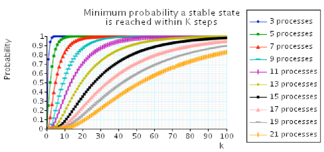
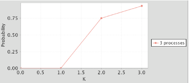
Figure 3: The minimum probability of reaching a stable configuration within K steps

We have a When propagator for the “when” and a When class for calling the propagator. A process when $C$ do $P$ is represented by two propagators: $C\leftrightarrow b$ (a reified propagator for the constraint $C$) and if $b$ then $P$ else $skip$ (the When propagator). The When propagator checks the value of $b$. If the value of $b$ is true, it calls the Execute method of $P$. Otherwise, it does not take any action. Figure 3 shows how to encode the process when $a=c$ do $P$ using our When propagator.

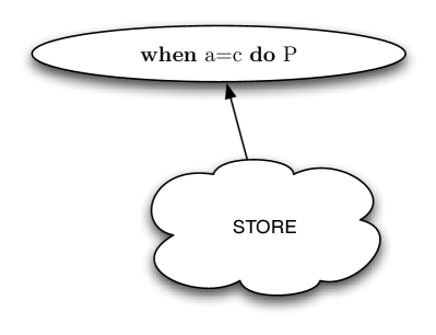
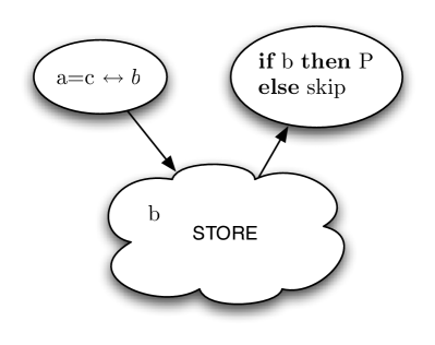
Figure 1: Example of the When propagator

We have a $\sum$ propagator …

3 Verification

Finally, we will extend the abstract machine to calculate a Discrete-Time Markov Chain (DTMC) and we will show its correctness.

3.0.1 Verification of non-probabilistic pntcc

A key aspect of pntcc is that it can be used for both, simulation and verification. Following, we define another abstract machine that calculates DTMCs instead of a simple sequence of outputs. Using the DTMC we can prove PCTL properties. This machine is an extension of pntccM and it is also based on the encoding given by Def. 12.

In order to execute $P$, the VerificationPntccM machine first need to encode $P$ into a suitable machine term. A machine term $V$ is a tuple composed by a FD constraint, a process, a DTMC and an integer.

Definition 25.

Syntax of VerificationPntccM.

V ::= $\langle A,B,C,j\rangle$, where

A is a Finite Domain constraint

B is a process defined in Def. 11

C is a DTMC (i.e., a tuple $\langle Q_{OBS},T_{OBS},LM\rangle$)

$j>0$

The following function is used to encode a pntcc process into a VerificationPntccM term to calculate a DTMC representing a $n$ time-units execution.

Definition 26.

Encoding a pntcc process into a VerificationPntccM term.

$(\ [P]\ )_{n,I}=\langle P_{1}\wedge I,P_{2},\langle n,\emptyset,(n,P_{1})\rangle n\rangle,$ where $(P_{1},P_{2})=[\ [P]\ ]_{T}$

Definition 27.

Reduction in VerificationPntccM.

$\langle A,B,C,i\rangle\longrightarrow^{I}\langle B_{1}\wedge I,B_{2},\\ \langle Q_{OBS}\cup\{i-1\},\gamma_{0},T_{OBS}\cup\{(i,i-1,1.0)\},LM\cup\{(B,B_{1}\wedge I)\}\rangle,i-1\rangle$
where $(B_{1},B_{2})=[\ [B]\ ]$, $\langle Q_{OBS},\gamma_{0},T_{OBS},LM\rangle=C$ and $i>0$

$\langle A,B,C,i\rangle\longrightarrow/\$  , when $i\leq 0$

Proposition 8.

Given a pntcc process $P$, the DTMC given by the first ? states of the DTMC($\langle P,true\rangle$) is an isomorph of the verification structure Ver(P,n)…

Proof.

The proof proceeds by induction DTMC($\langle P,true\rangle$) ∎

4 Applications

4.1 Herman’s Stabilization protocol

4.2 Description

A self-stabilising protocol for a network of processes is a protocol which, when started from some possibly illegal start configuration, returns to a legal/stable configuration without any outside intervention within some finite number of steps. For further details on self-stabilisation see here.

In each of the protocols we consider, the network is a ring of identical processes. The stable configurations are those where there is exactly one process designated as ”privileged” (has a token). This privilege (token) should be passed around the ring forever in a fair manner.

For each of the protocols, we compute the minimum probability of reaching a stable configuration and the maximum expected time (number of steps) to reach a stable configuration (given that the above probability is 1) over every possible initial configuration of the protocol.

The first protocol we consider is due to Herman [Her90]. The protocol operates synchronously, the ring is oriented, and communication is unidirectional in the ring. In this protocol the number of processes in the ring must be odd.

Each process in the ring has a local boolean variable xi, and there is a token in place i if xi=x(i-1). In a basic step of the protocol, if the current values of xi and x(i-1) are equal, then it makes a (uniform) random choice as to the next value of xi, and otherwise it sets it equal to the current value of x(i-1).

4.3 Simulation

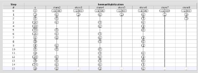
Figure 2: simulation

"Ntccrt Simulation"
""
""
"Time Unit \# 0"
"Number of processes= 7"
""
"Variables Value (Only those specified are printed)"
"num\_tokens"
"3"
"x1"
"0"
"x2"
"0"
"x3"
"0"
"changex1"
"1"
"changex2"
"1"
"changex3"
"1"
"..........................................."
""
"Time Unit # 1"
"Number of processes= 18"
""
"Variables Value (Only those specified are printed)"
"num_tokens"
"1"
"x1"
"1"
"x2"
"0"
"x3"
"0"

"..........................................."
""
"Time Unit # 2"
"Number of processes= 22"
""
"Variables Value (Only those specified are printed)"
"num_tokens"
"1"
"x1"
"0"
"x2"
"1"
"x3"
"1"
"changex1"
"1"
"changex2"
"1"
"changex3"
"1"
"..........................................."
""
"Time Unit # 3"
"Number of processes= 26"
""
"Variables Value (Only those specified are printed)"
"num_tokens"
"1"
"x1"
"1"
"x2"
"0"
"x3"
"0"
"changex1"
"1"
"changex2"
"1"
"changex3"
"1"
"..........................................."
""
"Time Unit # 4"
"Number of processes= 30"
""
"Variables Value (Only those specified are printed)"
"num_tokens"
"1"
"x1"
"0"
"x2"
"1"
"x3"
"1"
"changex1"
"1"
"changex2"
"1"
"changex3"
"1"
"..........................................."
""
"Time Unit # 5"
"Number of processes= 34"
""
"Variables Value (Only those specified are printed)"
"num_tokens"
"1"
"x1"
"1"
"x2"
"0"
"x3"
"0"
"changex1"
"1"
"changex2"
"1"
"changex3"
"1"
"..........................................."
""
"Time Unit # 6"
"Number of processes= 38"
""
"Variables Value (Only those specified are printed)"
"num_tokens"
"1"
"x1"
"0"
"x2"
"1"
"x3"
"1"
"changex1"
"1"
"changex2"
"1"
"changex3"
"1"
"..........................................."
""
"Time Unit # 7"
"Number of processes= 42"
""
"Variables Value (Only those specified are printed)"
"num_tokens"
"1"
"x1"
"1"
"x2"
"0"
"x3"
"1"
"changex1"
"1"
"changex2"
"1"
"changex3"
"1"
"..........................................."
""
"Time Unit # 8"
"Number of processes= 46"
""
"Variables Value (Only those specified are printed)"
"num_tokens"
"1"
"x1"
"1"
"x2"
"1"
"x3"
"0"
"changex1"
"1"
"changex2"
"1"
"changex3"
"1"
"..........................................."
NIL
T

CL-USER 10 ¿

4.4 Model Checking

We first check the correctness of the protocol, namely that:

From any configuration, a stable configuration is reached with probability 1

We then studied the following quantitative properties:

The minimum probability of reaching a stable configuration within K steps (from any configuration)

4.5 zig-zagging problem

4.5.1 description

Zigzagging [free99] is task on which a robot can go either foward, left, or right but (1) it cannot go forward if its preceding action was to go forward, (2) it cannot turn right if its second-last action was to go right, and (3) it cannot turn left if its second-last action was to go left. (frank thesis - page 105)

Valencia models this problem by using cells $a_{1}$ and $a_{2}$ to “look back” and three different distinct constrats $f,r,l\in D-\{0\}$ and the predicate symbols forward, right, left.

GoF
GoR
GoL
Zigzag
GoZigZag

Valencia verifies that GoZigzag $models$ $square(romboright...$.

4.5.2 simulation

Frank’s style

"Ntccrt Simulation"
""
""
"Time Unit # 0"
"Number of processes= 3"
""
"Variables Value (Only those specified are printed)"
"direction"
"1"
"a1"
"0"
"a2"
"0"
"changea1"
"1"
"changea2"
"1"
"..........................................."
""
"Time Unit # 1"
"Number of processes= 9"
""
"Variables Value (Only those specified are printed)"
"direction"
"3"
"a1"
"1"
"a2"
"0"
"changea1"
"1"
"changea2"
"1"
"..........................................."
""
"Time Unit # 2"
"Number of processes= 11"
""
"Variables Value (Only those specified are printed)"
"direction"
"1"
"a1"
"3"
"a2"
"1"
"changea1"
"1"
"changea2"
"1"
"..........................................."
""
"Time Unit # 3"
"Number of processes= 13"
""
"Variables Value (Only those specified are printed)"
"direction"
"2"
"a1"
"1"
"a2"
"3"
"changea1"
"1"
"changea2"
"1"
"..........................................."
""
"Time Unit # 4"
"Number of processes= 15"
""
"Variables Value (Only those specified are printed)"
"direction"
"2"
"a1"
"2"
"a2"
"1"
"changea1"
"1"
"changea2"
"1"
"..........................................."
""
"Time Unit # 5"
"Number of processes= 17"
""
"Variables Value (Only those specified are printed)"
"direction"
"1"
"a1"
"2"
"a2"
"2"
"changea1"
"1"
"changea2"
"1"
"..........................................."
""
"Time Unit # 6"
"Number of processes= 19"
""
"Variables Value (Only those specified are printed)"
"direction"
"3"
"a1"
"1"
"a2"
"2"
"changea1"
"1"
"changea2"
"1"
"..........................................."
""
"Time Unit # 7"
"Number of processes= 21"
""
"Variables Value (Only those specified are printed)"
"direction"
"3"
"a1"
"3"
"a2"
"1"
"changea1"
"1"
"changea2"
"1"
"..........................................."
""
"Time Unit # 8"
"Number of processes= 23"
""
"Variables Value (Only those specified are printed)"
"direction"
"1"
"a1"
"3"
"a2"
"3"
"changea1"
"1"
"changea2"
"1"
"..........................................."
""
"Time Unit # 9"
"Number of processes= 25"
""
"Variables Value (Only those specified are printed)"
"direction"
"2"
"a1"
"1"
"a2"
"3"
"changea1"
"1"
"changea2"
"1"
"..........................................."
""
"Time Unit # 10"
"Number of processes= 27"
""
"Variables Value (Only those specified are printed)"
"direction"
"2"
"a1"
"2"
"a2"
"1"
"changea1"
"1"
"changea2"
"1"
"..........................................."
""
"Time Unit # 11"
"Number of processes= 29"
""
"Variables Value (Only those specified are printed)"
"direction"
"3"
"a1"
"2"
"a2"
"2"
"changea1"
"1"
"changea2"
"1"
"..........................................."
""
"Time Unit # 12"
"Number of processes= 31"
""
"Variables Value (Only those specified are printed)"
"direction"
"1"
"a1"
"3"
"a2"
"2"
"changea1"
"1"
"changea2"
"1"
"..........................................."

My way

"Ntccrt Simulation"
""
"SKIP:: cella1 -11::"
"SKIP:: zigzag -11::"
"SKIP:: GoR -11::"
"SKIP:: Exchange value ! -11::"
"SKIP:: exch0 -11::"
"SKIP:: I will call exch_aux0 -11::"
""
"Time Unit # 0"
"Number of processes= 5"
""
"Variables Value (Only those specified are printed)"
"direction"
"2"
"a1"
"0"
"a2"
"0"
"changea1"
"1"
"changea2"
"1"
"x"
"0"
"y"
"0"
"changex"
"1"
"changey"
"[-2147483645..2147483645]"
"..........................................."
"SKIP:: zigzag -11::"
"SKIP:: value changes!!!! -11::"
"SKIP:: cella1 -11::"
"SKIP:: GoF -11::"
"SKIP:: Exchange value ! -11::"
"SKIP:: exch2 -11::"
""
"Time Unit # 1"
"Number of processes= 15"
""
"Variables Value (Only those specified are printed)"
"direction"
"1"
"a1"
"2"
"a2"
"0"
"changea1"
"1"
"changea2"
"1"
"x"
"1"
"y"
"0"
"changex"
"[-2147483645..2147483645]"
"changey"
"1"
"..........................................."
"SKIP:: zigzag -11::"
"SKIP:: cella1 -11::"
"SKIP:: GoL -11::"
"SKIP:: Exchange value ! -11::"
"SKIP:: exch1 -11::"
""
"Time Unit # 2"
"Number of processes= 18"
""
"Variables Value (Only those specified are printed)"
"direction"
"3"
"a1"
"1"
"a2"
"2"
"changea1"
"1"
"changea2"
"1"
"x"
"1"
"y"
"1"
"changex"
"1"
"changey"
"[-2147483645..2147483645]"
"..........................................."
"SKIP:: zigzag -11::"
"SKIP:: cella1 -11::"
"SKIP:: GoF -11::"
"SKIP:: Exchange value ! -11::"
"SKIP:: exch3 -11::"
""
"Time Unit # 3"
"Number of processes= 21"
""
"Variables Value (Only those specified are printed)"
"direction"
"1"
"a1"
"3"
"a2"
"1"
"changea1"
"1"
"changea2"
"1"
"x"
"0"
"y"
"1"
"changex"
"[-2147483645..2147483645]"
"changey"
"1"
"..........................................."
"SKIP:: zigzag -11::"
"SKIP:: cella1 -11::"
"SKIP:: GoR -11::"
"SKIP:: Exchange value ! -11::"
"SKIP:: exch1 -11::"
""
"Time Unit # 4"
"Number of processes= 24"
""
"Variables Value (Only those specified are printed)"
"direction"
"2"
"a1"
"1"
"a2"
"3"
"changea1"
"1"
"changea2"
"1"
"x"
"0"
"y"
"2"
"changex"
"1"
"changey"
"[-2147483645..2147483645]"
"..........................................."
"SKIP:: zigzag -11::"
"SKIP:: cella1 -11::"
"SKIP:: GoR -11::"
"SKIP:: Exchange value ! -11::"
"SKIP:: exch2 -11::"
""
"Time Unit # 5"
"Number of processes= 27"
""
"Variables Value (Only those specified are printed)"
"direction"
"2"
"a1"
"2"
"a2"
"1"
"changea1"
"1"
"changea2"
"1"
"x"
"1"
"y"
"2"
"changex"
"1"
"changey"
"[-2147483645..2147483645]"
"..........................................."
"SKIP:: zigzag -11::"
"SKIP:: cella1 -11::"
"SKIP:: GoF -11::"
"SKIP:: Exchange value ! -11::"
"SKIP:: exch2 -11::"
""
"Time Unit # 6"
"Number of processes= 30"
""
"Variables Value (Only those specified are printed)"
"direction"
"1"
"a1"
"2"
"a2"
"2"
"changea1"
"1"
"changea2"
"1"
"x"
"2"
"y"
"2"
"changex"
"[-2147483645..2147483645]"
"changey"
"1"
"..........................................."
"SKIP:: zigzag -11::"
"SKIP:: cella1 -11::"
"SKIP:: GoL -11::"
"SKIP:: Exchange value ! -11::"
"SKIP:: exch1 -11::"
""
"Time Unit # 7"
"Number of processes= 33"
""
"Variables Value (Only those specified are printed)"
"direction"
"3"
"a1"
"1"
"a2"
"2"
"changea1"
"1"
"changea2"
"1"
"x"
"2"
"y"
"3"
"changex"
"1"
"changey"
"[-2147483645..2147483645]"

4.5.3 Model checking

Frank style

// The robot does not go foward twice ”init” =¿ P¡=0 [F store2 = 1 & store3 = 1]

// The robot does not go right more than twice ”init” =¿ P¡=0 [F store2=2 & store3 = 2 & store4 = 2]

//The robot does not go left more than twice ”init” =¿ P¡=0 [F store2=3 & store3 = 3 & store4 = 3]

// The robot always makes a good move ”init” =¿ P¿=1 [F (store2 !=1 — store3 !=1) & (store2 != 2 — store3 != 2 — store4 != 2) & (store2 != 3 — store3 != 3 — store4 != 3)]

My way

Probability distribution for x,y positions

const x; const y; P ? [F store7 = x & store8 = y]

References

- [AAO+09] Jesús Aranda, Gérard Assayag, Carlos Olarte, Jorge A. Pérez, Camilo Rueda, Mauricio Toro, and Frank D. Valencia. An overview of FORCES: an INRIA project on declarative formalisms for emergent systems. In Patricia M. Hill and David Scott Warren, editors, Logic Programming, 25th International Conference, ICLP 2009, Pasadena, CA, USA, July 14-17, 2009. Proceedings, volume 5649 of Lecture Notes in Computer Science, pages 509–513. Springer, 2009.
- [ADCT11] Antoine Allombert, Myriam Desainte-Catherine, and Mauricio Toro. Modeling temporal constrains for a system of interactive score. In Gérard Assayag and Charlotte Truchet, editors, Constraint Programming in Music, chapter 1, pages 1–23. Wiley, 2011.
- [MPT17] Juan David Arcila Moreno, Santiago Passos, and Mauricio Toro. On-line assembling mitochondrial DNA from de novo transcriptome. CoRR, abs/1706.02828, 2017.
- [ORS+11] Carlos Olarte, Camilo Rueda, Gerardo Sarria, Mauricio Toro, and Frank Valencia. Concurrent Constraints Models of Music Interaction. In Gérard Assayag and Charlotte Truchet, editors, Constraint Programming in Music, chapter 6, pages 133–153. Wiley, Hoboken, NJ, USA., 2011.
- [PAZ98] M. Puckette, T. Apel, and D. Zicarelli. Real-time audio analysis tools for Pd and MSP. In Proceedings of the International Computer Music Conference., 1998.
- [PFATT16] C. Patiño-Forero, M. Agudelo-Toro, and M. Toro. Planning system for deliveries in Medellín. ArXiv e-prints, November 2016.
- [PT13] Anna Philippou and Mauricio Toro. Process Ordering in a Process Calculus for Spatially-Explicit Ecological Models. In Proceedings of MOKMASD’13, LNCS 8368, pages 345–361. Springer, 2013.
- [PTA13] Anna Philippou, Mauricio Toro, and Margarita Antonaki. Simulation and Verification for a Process Calculus for Spatially-Explicit Ecological Models. Scientific Annals of Computer Science, 23(1):119–167, 2013.
- [RML18] Mazo Raul, Toro Mauricio, and Cobaleda Luz. Definicion de la arquitectura de referencia de un dominio: de la elucidacion al modelado. In Raul Mazo, editor, Guia para la adopcion industrial de lineas de productos de software, pages 193–210. Editorial Eafit, 2018.
- [RPT17] Juan Manuel Ciro Restrepo, Andrés Felipe Zapata Palacio, and Mauricio Toro. Assembling sequences of DNA using an on-line algorithm based on debruijn graphs. CoRR, abs/1705.05105, 2017.
- [SS06] Christian Schulte and Peter J. Stuckey. Efficient constraint propagation engines. CoRR, abs/cs/0611009, 2006.
- [TAAR09] Mauricio Toro, Carlos Agón, Gérard Assayag, and Camilo Rueda. Ntccrt: A concurrent constraint framework for real-time interaction. In Proc. of ICMC ’09, Montreal, Canada, 2009.
- [TDC10] Mauricio Toro and Myriam Desainte-Catherine. Concurrent constraint conditional branching interactive scores. In Proc. of SMC ’10, Barcelona, Spain, 2010.
- [TDCB10] Mauricio Toro, Myriam Desainte-Catherine, and P. Baltazar. A model for interactive scores with temporal constraints and conditional branching. In Proc. of Journées d’Informatique Musical (JIM) ’10, May 2010.
- [TDCC12] Mauricio Toro, Myriam Desainte-Catherine, and Julien Castet. An extension of interactive scores for multimedia scenarios with temporal relations for micro and macro controls. In Proc. of Sound and Music Computing (SMC) ’12, Copenhagen, Denmark, July 2012.
- [TDCC16] MAURICIO TORO, MYRIAM DESAINTE-CATHERINE, and JULIEN CASTET. An extension of interactive scores for multimedia scenarios with temporal relations for micro and macro controls. European Journal of Scientific Research, 137(4):396–409, 2016.
- [TDCR14] Mauricio Toro, Myriam Desainte-Catherine, and Camilo Rueda. Formal semantics for interactive music scores: a framework to design, specify properties and execute interactive scenarios. Journal of Mathematics and Music, 8(1):93–112, 2014.
- [Tor08] Mauricio Toro. Exploring the possibilities and limitations of concurrent programming for multimedia interaction and graphical representations to solve musical csp’s. Technical Report 2008-3, Ircam, Paris.(FRANCE), 2008.
- [Tor09a] Mauricio Toro. Probabilistic Extension to the Factor Oracle Model for Music Improvisation. Master’s thesis, Pontificia Universidad Javeriana Cali, Colombia, 2009.
- [Tor09b] Mauricio Toro. Towards a correct and efficient implementation of simulation and verification tools for probabilistic ntcc. Technical report, Pontificia Universidad Javeriana, May 2009.
- [Tor10] Mauricio Toro. Structured interactive musical scores. In Manuel V. Hermenegildo and Torsten Schaub, editors, Technical Communications of the 26th International Conference on Logic Programming, ICLP 2010, July 16-19, 2010, Edinburgh, Scotland, UK, volume 7 of LIPIcs, pages 300–302. Schloss Dagstuhl - Leibniz-Zentrum fuer Informatik, 2010.
- [Tor12] Mauricio Toro. Structured Interactive Scores: From a simple structural description of a multimedia scenario to a real-time capable implementation with formal semantics . PhD thesis, Univeristé de Bordeaux 1, France, 2012.
- [Tor15] Mauricio Toro. Structured interactive music scores. CoRR, abs/1508.05559, 2015.
- [Tor16a] M. Toro. Probabilistic Extension to the Concurrent Constraint Factor Oracle Model for Music Improvisation. ArXiv e-prints, February 2016.
- [Tor16b] Mauricio Toro. Probabilistic Extension to the Concurrent Constraint Factor Oracle Model for Music Improvisation . Inteligencia Artificial, 57(19):37–73, 2016.
- [Tor18] Mauricio Toro. CURRENT TRENDS AND FUTURE RESEARCH DIRECTIONS FOR INTERACTIVE MUSIC. Journal of Theoretical and Applied Information Technology, 69(16):5569–5606, 2018.
- [TPA+16] Mauricio Toro, Anna Philippou, Sair Arboleda, María Puerta, and Carlos M. Vélez S. Mean-field semantics for a process calculus for spatially-explicit ecological models. In César A. Muñoz and Jorge A. Pérez, editors, Proceedings of the Eleventh International Workshop on Developments in Computational Models, Cali, Colombia, October 28, 2015, volume 204 of Electronic Proceedings in Theoretical Computer Science, pages 79–94. Open Publishing Association, 2016.
- [TPKS14] Mauricio Toro, Anna Philippou, Christina Kassara, and Spyros Sfenthourakis. Synchronous parallel composition in a process calculus for ecological models. In Gabriel Ciobanu and Dominique Méry, editors, Proceedings of the 11th International Colloquium on Theoretical Aspects of Computing - ICTAC 2014, Bucharest, Romania, September 17-19, volume 8687 of Lecture Notes in Computer Science, pages 424–441. Springer, 2014.
- [TRAA15] MAURICIO TORO, CAMILO RUEDA, CARLOS AGÓN, and GÉRARD ASSAYAG. Ntccrt: A concurrent constraint framework for soft real-time music interaction. Journal of Theoretical & Applied Information Technology, 82(1), 2015.
- [TRAA16] MAURICIO TORO, CAMILO RUEDA, CARLOS AGÓN, and GÉRARD ASSAYAG. Gelisp: A framework to represent musical constraint satisfaction problems and search strategies. Journal of Theoretical & Applied Information Technology, 86(2), 2016.