On the Calculation of Resonances in Pre-Born–Oppenheimer Molecular Structure Theory
Abstract
The main motivation for this work is the exploration of rotational-vibrational states corresponding to electronic excitations in a pre-Born–Oppenheimer quantum theory of molecules. These states are often embedded in the continuum of the lower-lying dissociation channel of the same symmetry, and thus are thought to be resonances. In order to calculate rovibronic resonances, the pre-Born–Oppenheimer variational approach of [J. Chem. Phys. 137, 024104 (2012)], based on the usage of explicitly correlated Gaussian functions and the global vector representation, is extended with the complex coordinate rotation method. The developed computer program is used to calculate resonance energies and widths for the three-particle positronium anion, Ps-, and the four-particle positronium molecule, Ps2. Furthermore, the excited bound and resonance rovibronic states of the four-particle H2 molecule are also considered. Resonance energies and widths are estimated for the lowest-energy resonances of H2 beyond the continuum.
Keywords: rovibronic energy level, predissociation, complex coordinate rotation method, Ps-, Ps2, H2
Eötvös University] Laboratory of Molecular Structure and Dynamics, Institute of Chemistry, Eötvös University, P.O. Box 32, H-1518, Budapest 112, Hungary
1 Introduction
The present work is devoted to conceptual and computational problems in pre-Born–Oppenheimer (pre-BO) molecular structure theory. Without the Born–Oppenheimer (BO) approximation,1, 2, 3 in a “pre-BO world”, we can gain in accuracy for the numerical results but loose a central paradigm for the well-accustomed concepts of chemistry. The reconstruction or interpretation of many common chemical concepts becomes a real challenge. One of these famous challenges, the problem of the quantum structure of molecules has been recognized long ago4, 5, 6, 7 and studied by many authors.8, 9, 10, 11, 12, 13, 14, 15, 16, 17, 18, 19, 20
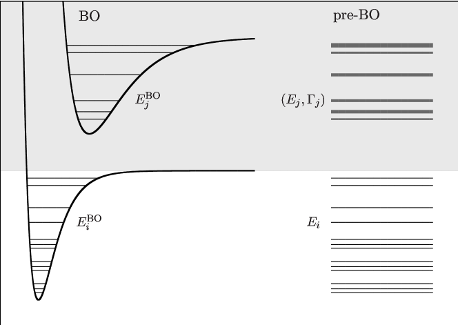
In the present work we address another challenge, the status of electronically excited rotational-vibrational states in a pre-BO quantum mechanical description. In a pre-BO description there are no electronic states with corresponding potential energy curves or surfaces on which the rotational-vibrational Schrödinger equation could be solved. In addition, rotational-vibrational states corresponding to electronic excitations are often embedded in the lowest-lying dissociation channel of the system, 1, prone to predissociation.21 These rovibronic states are thus accessible in a pre-BO description only as resonances. These rovibronic resonances are characterized with some energy and width corresponding to a finite non-radiative (predissociative) lifetime. Our aim is to explore how these properties can be calculated in a pre-BO approach.
As to the numerical results, there are practical approaches used for the calculation of quasi-bound states in molecular science 22, 23, 24. The stabilization technique, a very simple computational tool has been used to identify resonances and to estimate the resonance energy25, 26, 27 and can also be extended to the calculations of the width.28, 29, 30, 31 The complex coordinate rotation method 32, 33, 34 is a neat mathematical approach for the calculation of the resonance energy and width, and has been used in several cases,23, 24 for example in rotational-vibrational calculations on a potential energy surface within the Born–Oppenheimer (BO) theory.35, 31 The usage of complex absorbing potentials 36, 37, 38 has been a popular technique in molecular spectroscopy and quantum reaction kinetics with many applications.39, 40, 41 There exist also more involved and specialized approaches, such as the solution of the Faddeev–Merkuriev integral equations. 42, 43
The present work is organized as follows. First, the necessary theoretical framework is described for the variational solution of the Schrödinger equation for bound states of few-particle systems. Then, this approach is extended for the identification and calculation of quasi-bound states. Next, numerical examples are presented for the three-particle Ps- and the four-particle Ps2. Finally, the description of excited bound and resonance rovibronic states of the four-particle H2 is explored. In the end, we finish with a summary and outlook.
2 Theory and computational strategy
The Schrödinger equation for an -particle system with masses and electric charges assigned to the particles is
| (1) |
with the non-relativistic quantum Hamiltonian in Hartree atomic units
| (2) |
written in laboratory-fixed Cartesian coordinates .
In the present work we use the bound-state variational approach of Ref. 44 and (a) combine it with the stabilization technique to quickly identify long-lived resonances; and (b) extend it with the complex coordinate rotation method to calculate resonance energies and widths.
2.1 Variational pre-BO calculations using explicitly correlated Gaussian functions and the global vector representation
The overall translation of the center of mass is eliminated by writing the kinetic energy operator in terms of Jacobi Cartesian coordinates and the translational kinetic energy of the center of mass is subtracted. As an alternative to this approach, the original laboratory-fixed Cartesian coordinates can be used throughout the calculations without any further coordinate transformation employing a special elimination technique for the overall translation during the evaluation of the matrix elements.45
The matrix representation of the translationally invariant Hamiltonian is constructed using a symmetry-adapted basis set defined as follows.
A basis function with the quantum numbers111 denotes here the total spatial (orbital plus rotational) angular momentum quantum number in agreement with the recommendations of the International Union of Pure and Applied Chemistry.46 We note that in Ref. 44 the symbol was used in the same sense. Furthermore, is the parity, which we call “natural” if and “unnatural” if . In this work we restrict the discussion to natural-parity states. The total spin quantum number for particles of type is . For example, and denote the total spin quantum numbers for the protons and the electrons, respectively. and ( label the particle type) is constructed as
| (3) |
where is the symmetrization and antisymmetrization operator for bosonic and fermionic-type particles, respectively. () is an operator permuting identical particles and if corresponds to an odd number of interchanges of fermions, otherwise, .
The spatial part of the basis functions with natural parity, , is constructed using explicitly correlated Gaussian functions47, 48, 49, 50, 51 and the global vector representation52, 53, 54 as
| (4) |
where the unit vector points in the direction of the global vector, . denote the th order th degree spherical harmonic function. The spin function, , is constructed from elementary spin functions so that the resulting function is an eigenfunction of and for each type of particles () with the quantum numbers .
Then, the resulting basis function has the quantum numbers of the non-relativistic quantum theory (it is “symmetry-adapted”) and contains free parameters, which can be optimized for an efficient description of the “internal structure” of a system. The free parameters of the spatial function, 4, are , : , and : with the restriction , which guarantees translational invariance. The spin functions used in this work do not contain any free parameters.
We only note here that for the positronium molecule, Ps2, as a special case studied in this work, the entire basis function was additionally adapted to the charge-conjugation symmetry of the electrons and the positrons.55, 56, 57
The matrix elements of the kinetic and potential energy operators corresponding to the basis functions with natural parity, 3–4, were evaluated with the pre-BO program according to Ref. 44.
Since the basis functions are not orthogonal we have to solve a generalized eigenvalue problem
| (5) |
to find the variationally optimal linear combination of the basis functions with the linear combination coefficients corresponding to the eigenvalue . The generalized eigenproblem is solved by introducing and , which simplifies the eigenvalue equation, 5, to . In our computations the Cholesky decomposition of for the evaluation of as well as the diagonalization of the real, symmetric transformed Hamiltonian matrix, , were carried out by using the LAPACK library routines.58
The computational efficiency and usefulness of the variational approach described depends on the parameterization of the basis functions (the choice of the values of , , for the basis functions ). For bound-state calculations we adopted the stochastic variational approach59, 60, 61, 62, 54 for the optimization of the basis function parameters. The (quasi-)optimization of the parameter set is a very delicate problem and our recipe includes the following details:44 (a) a system-adapted random number generator is constructed using a sampling-importance resampling strategy for the generation of trial parameter sets; (b) the acceptance criterion of the generated trial values is based on the linear independence condition and the energy minimization requirement (relying on the variational principle); (c) the selected parameters are fine-tuned using a simple random walk approach or Powell’s method63.
Furthermore, once a parameter set has been selected or optimized for a system with some quantum numbers it can be used, “transferred”, to parameterize basis functions for the same system with different quantum numbers (“parameter transfer approach”). It is important to emphasize that the basis functions are not transferred, since they have different mathematical form for different quantum numbers, but only the parameter set is taken over from one calculation to another.
2.2 Calculation of resonances
The bound-state pre-BO approach described was extended for the calculation of resonance states as follows. First of all, without any change of the computer program, we looked for the quasi-stabilization of higher-energy eigenvalues (higher than the lowest-energy threshold) of the real eigenvalue problem. This application of the stabilization technique25, 26, 27 is a simple, practical test for identifying possible quasi-bound states and was found to be useful as a first check of the higher-energy eigenspectrum. By making full use of the stabilization theory both the resonance energies and widths could be calculated from consecutive diagonalization of the (real) Hamiltonian matrix corresponding to increasing number of basis functions, which cover increasing boxes of the configuration space.28, 29, 30, 31
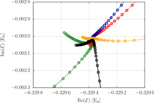
Instead of using this approach, the complex coordinate rotation method (CCRM) 32, 33, 34, 23, 24 was implemented for the calculation of resonance parameters, energies and widths. The resonance parameters were determined by identifying stabilization points in the complex plane with respect to the coordinate rotation angle and (the size and parameterization of) the basis set. The localized real part of the eigenvalue, , was taken to be the resonance energy, and the imaginary part provided the resonance width, , which is inversely proportional to the lifetime, .22
Implementation of the complex coordinate rotation method for the Coulomb Hamiltonian
The complex scaling of the coordinates translates to the replacement of the Hamiltonian with
| (6) |
The matrix representation of is constructed with the matrices of and evaluated by the pre-BO program 44. Then, the eigenvalue equation for reads as
| (7) |
where is the overlap matrix of the (linearly independent) set of basis functions. is eliminated from the equation similarly to the case of the real generalized eigenproblem, 5,
| (8) |
with
| (9) |
and
| (10) |
The complex symmetric eigenvalue problem, 8, is solved using the LAPACK library routines.58
3 Numerical results
The first numerical applications of our implementation were carried out for the notoriously non-adiabatic positronium anion, Ps, and for the positronium molecule, Ps. The reason for the choice of these systems was of technical nature: we observed in bound-state calculations 44 that it was straightforward to find an appropriate parameterization of the basis set for the positronium complexes. Furthermore, comparison of the results with earlier calculations42, 64, 27, 65 allowed us check the developed computational methods and gain experience in the localization of the real and imaginary parts of the complex eigenvalues using the complex coordinate rotation method.
While for the bound-state calculations the basis function parameters were optimized for the lowest-energy level(s) using the variational principle, this handy optimization criterion was not available in the CCRM calculations. Thus, we used optimized bound-state basis sets and enlarged them with linearly independent basis functions for the estimation of the resonance parameters.
Next, we investigated the calculation of some of the excited states of the H2 molecule. The construction of a reasonably good parameterization for the basis set has turned out to be a challenge. Nevertheless, we describe the essence of our observations and give calculated resonance energy values and approximate widths for the lowest-lying excited states beyond the repulsive electronic state embedded in the H(1)+H(1) continuum.
3.1 Ps-
In 1 bound- and resonance-state parameters (, ) are collected, which were obtained in this work. The basis sets were generated using the energy minimization and the linear independence conditions using a random number generator set up following the strategy described in Ref. 44. The parameters for the largest basis sets used during the calculations are given in the Supporting Information. The generated basis sets were apparently large and flexible enough to obtain resonance states not only beyond the first, but also beyond the second, and the third dissociation channels which correspond to , , and , respectively. As to the accuracy, the (real) variational principle, directly applicable for bound states, is not useful for the assessment of the resonance parameters. Instead, we used benchmarks available in the literature resulting from extensive three-body calculations using Pekeris-type wave functions with one and two length scales64 and from the solution of the Fadeev–Merkuriev integral equations for three-body systems.42
First of all, the present results and the literature data are in satisfactory agreement. Our results could be certainly improved by running more extensive calculations with larger basis sets. Instead of going in this direction, a careful comparison is carried out with the reference data in order to learn about the accuracy and convergence behavior of our approach. The results are often in excellent agreement with the benchmarks but in some cases the lifetimes are orders of magnitude off. It can be observed that the calculated lifetimes are worse when the real part of the complex energy was determined less accurately (and given to less significant digits in 1). The inaccuracy appears in both the real and the imaginary parts and is about of the same order of magnitude compared to the absolute value of the complex energy. Thus, if the widths are expected to be very small and the real part can be determined only to a few digits, the width should be considered only as a rough estimate to its exact value. This observation can be used later in this work also for the assessment of the calculations carried out for the four-particle Ps2 and H2.
| b | c | c | d | d | Ref. |
|---|---|---|---|---|---|
| e | e | 66 | |||
| \cdashline1-6 | |||||
| 64 | |||||
| 64 | |||||
| 42 | |||||
| \cdashline1-6 | |||||
| 64 | |||||
| 64 | |||||
| 42 | |||||
| \cdashline1-6 | |||||
| 64 | |||||
| \cdashline1-6 | |||||
| 64 | |||||
| 42 | |||||
| \cdashline1-6 | |||||
| 64 | |||||
| 42 | |||||
| \cdashline1-6 | |||||
| 42 |
a The dissociation threshold energies, in Eh, accessible for both the and 1 states are , , and .
b and : total spatial angular momentum quantum number, parity, and total spin quantum number of the electrons, respectively.
c and : resonance energy and width with calculated in this work.
e Bound state.
3.2 Ps2
Our next test case was the four-particle positronium molecule, Ps. Resonances of the positronium molecule have recently attracted attention 67, 65, 27. Ps2 has few bound states, and thus a detailed spectroscopic investigation of its structure and dynamics is possible only through the detection and analysis of its quasi-bound states.
In our list of numerical examples, the positronium molecule is unique because, in addition to the spatial symmetries, its Hamiltonian is invariant under the conjugation of the electric charges. In order to account for this additional property, the basis functions, 3–4, were adapted also to the charge conjugation symmetry.68, 65, 55, 56, 57 As a result, the total symmetry-adapted basis functions and also the calculated wave functions are not necessarily eigenfunctions for the total spin angular momentum of the electrons or that of the positrons, or . Nevertheless, the total spatial angular momentum quantum number, , the parity, , as well as the charge-conjugation parity, or , are always good quantum numbers.
The parameterization strategy of the basis set was similar to that used for Ps-: we employed (a) the energy minimization condition for the lowest-energy eigenvalue; and (b) the linear independence condition for the generation of new basis function parameters. The parameter sets used in the largest calculations are given in the Supporting Information.
The bound and resonance states calculated with total spatial angular momentum quantum number and parity are collected in 2. Considering all possible charge conjugation and spin functions, we obtained only three bound states in agreement with the literature.69, 27, 65 Two of the three calculated bound states substantially improve on the best available results.65 It is interesting to note that the bound state with Eh ( and ) is bound only due to the charge-conjugation symmetry of the electrons and the positrons. The localization of the energy and width for the lowest-energy resonance state of Ps2 is shown in 2. The calculated resonance positions are in good agreement with the literature. In some cases our results might even improve on the best available data,27, 65 although there is no such a direct criterion for the assessment of the accuracy of the resonance parameters as the variational principle for bound states.
a For the five symmetry blocks with different quantum numbers and
labels the lowest accessible thresholds are
Ps(1S)+Ps(1S),
Ps(1S)+Ps(2P),
Ps(1S)+Ps(2P),
Ps(1S)+Ps(1S),
Ps(1S)+Ps(2S,2P), respectively.68
The corresponding energies, in Eh, are
and
.
(The black and gray coloring is used to help the orientation.)
b and : total spatial angular momentum quantum number,
parity, and charge conjugation quantum number, respectively.
c and : total spin quantum numbers for the electrons and the positrons, respectively.
In the last symmetry block, and , are not good quantum numbers
because these spin states are coupled due to the charge-conjugation symmetry of the Hamiltonian.
d and :
resonance energy and width with calculated in this work.
e and :
resonance energy and width with taken from Ref. 65.
f Bound states.
3.3 Toward the calculation of rovibronic resonances of H2
Next, our goal was to explore how the lowest-lying resonance states of H2 can be calculated in a pre-Born–Oppenheimer quantum mechanical approach. It could be anticipated that one of the major challenges in this undertaking would be the parameterization of the basis functions, which was already in the bound-state calculations more demanding for H2 than for Ps2.44 In the bound-state calculations the optimized parameters were fine-tuned in repeated cycles. The entire parameter selection and optimization procedure relied on the variational principle and the minimization of the energy.
According to the spatial and permutational symmetry properties of the H2 molecule, there are four different blocks with natural parity
-
B1:
“ block”: ;
-
B2:
“ block”: ;
-
B3:
“ block”: ;
-
B4:
“ block”: ,
which can be calculated in independent runs with our computer program using basis functions with the appropriate quantum numbers, 3–4. The lowest-energy levels of the first three blocks correspond to bound states, while the last block starts with the H(1)+H(1) continuum. In the BO picture the electronic state is repulsive 70 and does not support any bound rotational-vibrational levels (see 3 and 3). Then, one of our goals was the identification of the lowest-energy quasi-bound states in the block.
During the calculation of the lowest-energy resonances of Ps2, the basis function parameters were generated randomly using a system-adapted random number generator.44 Unfortunately, this simple strategy for the H2 resonances was not useful.
The energy minimization criterion for the lowest (few) eigenstates was not useful neither, since it resulted only in the accumulation of functions near the H(1)+H(1) limit, the lowest energy levels in the block, and the higher-lying quasi-bound states were not at all described by the basis sets generated in this way.
Then, our alternative working strategy was the usage of the parameter transfer approach (described in Section “Theory and computational strategy” and in Ref. 44). In this approach a parameter set optimized for a bound state with some quantum numbers, “state ”, is used to parameterize the basis functions corresponding to another set of quantum numbers and used to calculate “state ”. It is important to emphasize that the mathematical form of the basis functions is defined by the selected values of the quantum numbers, 3–4, and thus not the basis functions but only the parameters are transferred from one calculation to another. Our qualitative understanding tells us that this parameter-transfer strategy is computationally useful if the internal structures of “state ” and “state ” are more or less similar. By inspecting the orientation chart of H2, 3, our idea was that the combination of the (natural-parity) bound-state optimized parameter sets could provide a parameterization good enough for the identification of the lowest-lying resonance states embedded in the continuum.
For this purpose, we used the parameters of basis functions optimized for the lowest-lying bound states with and angular momentum quantum numbers corresponding to the , , and blocks using the sampling-importance resampling strategy of Ref. 44 and Powell’s method63 for the fine-tuning of each basis function. As a result of these calculations, we obtained a parameter set large enough for basis functions. In addition, basis functions were generated and less tightly optimized for the lowest-energy levels of the block with and 1. Using this large parameter set, , basis functions were constructed for all possible quantum numbers of the four blocks, B1–B4, with and 2. In each case the resulting basis set was found to be linearly independent. The complete parameter set is given in the Supporting Information. The proton-electron ratio was throughout the calculations.71
Bound-state energy levels
The lowest-lying energy values obtained with for the different quantum numbers are collected in 3, and are in good agreement with the best available non-relativistic results in the literature. The energy values of the electronic and vibrational ground states with and are larger by only less than nEh than the theoretical results of Ref. 72.
For all three calculated levels our energy values are lower by more than compared to the results of Ref. 73 obtained in close-coupling calculations using adiabatic potential energy curves and non-adiabatic couplings for six electronic states. We also note that for the lowest-lying vibrational level of there is a “variational-perturbational” estimate given in Table 3 of Ref. 73, which was anticipated to be more accurate, and thus it was the recommended value for this level in the article, though not a strict upper bound to the exact value. It was obtained not in the six-state close-coupling calculations, but as a result of two-state close-coupling calculations with the potentials and couplings of Ref. 73, incremented with a non-adiabatic correction term.74 This term value translates to the energy value Eh based on the explanation given below Eq. (13) of Ref. 73. An earlier non-adiabatic estimate75 (not upper bound) for this energy level was Eh calculated using the adiabatic energy and a correction to the BO potential76 incremented by a non-adiabatic correction.74 For comparison, the pre-Born–Oppenheimer energy calculated in the present work (in a fully variational procedure) is Eh (3).
In the case of the energy levels the presented energy values obtained in this work are lower than the lowest energies values published77.
Based on this overview, we can conclude that the parameter set, , performs well for the lowest-lying bound-state energy levels and also contains basis functions optimized for an approximate description of the H(1)+H(1) continuum. Then, we can hope that the application of this parameter set in the CCRM calculations for the description of the related or just energetically nearby-lying quasi-bound states will be useful.
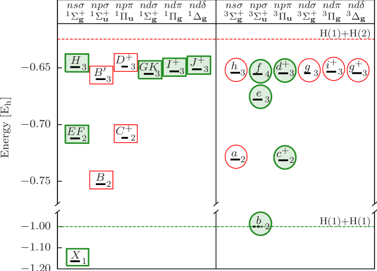
Electronically excited bound and resonance rovibronic states
In the orientation chart of H2, 3, the electronic states are collected below the H(1)+H(2) dissociation threshold known from the literature78, 79 (only natural-parity states are considered). Although in our calculations there are no potential energy curves corresponding to electronic states, these conventional electronic-state labels help the orientation and the reference to the calculated energy levels. In the figure those states which are coupled by symmetry and calculated in the same block are highlighted similarly (green or red color and oval or rectangular marking) corresponding to the B1–B4 blocks introduced earlier this section. This coupling is included in the calculations automatically by specifying the total spatial (orbital plus rotational) angular momentum, parity, and spin quantum numbers. The empty ellipses and rectangles indicate bound states, while the shaded signs are for resonance states embedded in their corresponding lowest-lying continuum (here: H(1)+H(1)).
We carried out calculations in all four blocks, B1–B4, with and 2 total spatial angular momentum quantum numbers and most of the states indicated in 3 could have been identified using the largest parameter set, . Unfortunately, the accuracy of the calculated energies often did not meet the level of spectroscopic accuracy,80 and thus we collect here only the essence of the calculations.
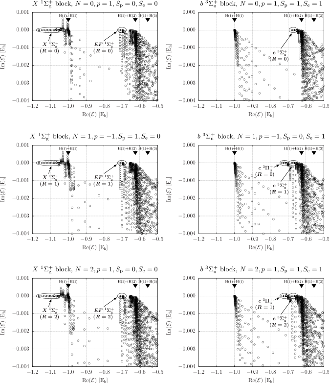
First of all, the most important qualitative results can be explained by inspecting 4 prepared for the “ block” and for the “ block”, B1 and B4. 4 shows a part of the eigenspectrum of the complex scaled Hamiltonian, of 6, corresponding to small values, , and the Eh interval of the real part of the eigenvalues.
In both cases the onset of the H(1)+H(1) continuum can be observed on the real axes at . In the block the bound rovibrational energy levels assignable to the electronic state line up on the real axis with (deviations from this value are due to the incomplete convergence only and the estimated stabilization points are on the real axis). In the block however we find no states below the H(1)+H(1) continuum, in agreement with the BO calculations 70. The next, H(1)+H(2) threshold corresponds to the energy value . Beyond the H(1)+H(1) but below the H(1)+H(2) thresholds stabilization points (with respect to the rotation angle and the basis set) were observed with small negative imaginary values, which were assigned (based on the real parts of the eigenvalues) to rotational-vibrational levels corresponding to the electronically excited states in their symmetry blocks (see 4 and also 3). The lack of any stabilization points beyond the H(1)+H(2) threshold can be explained with the limited size and flexibility of the basis set.
It can be observed in 4 in the block that a group of stabilization points appear for and , which are not present for . These points for and were assigned to the rotational-vibrational states with and 1 rotational angular momentum quantum numbers of the electronic state, respectively. This result demonstrates that the coupling of the rotational and orbital angular momenta are automatically included in the calculations by specifying only the total spatial angular momentum quantum number, .
Finally, we note that the H(1)+H(1) continuum does not couple neither to the “ block” nor to the “ block”, and in these cases the lowest-lying continuum corresponds to the H(1)+H(2) dissociation channel (3).
Numerical results for the resonance energies and widths
In 4 numerical results are given obtained for the “ block”, B4, for the lowest-lying rotational-vibrational levels with , and 2 corresponding to the () and to the () electronic-state labels. These rovibronic levels are embedded in the H(1)+H(1) continuum, and thus they are considered as rovibronic resonances.
The real energy values are in satisfactory agreement with the experimental results.81 We consider however the given imaginary parts as estimates to their accurate values, and all we can conclude at this point is that the obtained imaginary parts are of the order of Eh, which corresponds to a predissociative lifetime, , of the order of ns. As it was explained earlier, it is difficult to assess the accuracy of the calculated resonance energies and widths, since there is no such a simple criterion as the (real) variational principle for bound states. According to our observations in the test calculations for Ps- (1), the relative errors in the real and imaginary parts with respect to the absolute value of the complex energy are similar. The accuracy of the pre-BO real energy values can be estimated here by their comparison with available experimental results. This observation also indicates that the resonance widths given in 4 should be considered as rough estimates.
Theoretical energy values are available in the literature calculated by Kołos and Rychlewski82, 70 and are also cited in 4. In Ref. 70 adiabatic rotational-vibrational energy levels were determined for the electronic state by calculating an accurate adiabatic potential energy curve and solving the corresponding rotational-vibrational Schrödinger equation. The theoretical reference value for the level was taken from Ref. 82, which was obtained by the calculation of an accurate BO potential energy curve and solving the corresponding vibrational Schrödinger equation. The resulting BO energy could be furthermore corrected for the -doubling, but the numerical value for this correction term was not clearly identifiable in Ref. 82. It would be interesting to see if nonadiabatic corrections can be calculated to these levels, for example using the recently developed nonadiabatic perturbation theory by Pachucki and Komasa.83, 72
The lifetimes of rotational-vibrational levels corresponding to the state were measured in delayed coincidence experiments,84 which include both the radiative and predissociative decay channels accessible from these levels. In the same work the competition of the two decay channels were investigated using ab initio (full configuration interaction electronic wave functions using Gaussian-type orbitals and an accurate adiabatic potential energy curve70) as well as quantum defect theory with a one-channel approximation.84 According to these calculations the predissociative lifetimes are of the order of s and ns for the and vibrational levels, respectively, for the state with . The lifetime of the lowest rotational-vibrational levels of the state were calculated using a simple perturbative model, which included the orbit-rotation interaction and used several approximations during the calculations.85 In a similar perturbative treatment86 the orbit-rotational coupling operator was included and accurate BO potential energy curves were used to describe the and states.87, 82 According to both the lifetime measurements88, 89 and the calculations85, 86 the predissociative lifetime of the lowest-lying rotational-vibrational levels of are of the order of 1 ns. Unfortunately, calculated energy levels were not reported in any of these theoretical work85, 86, 84 on the predissociative lifetimes of the and states, which makes comparison of the results more difficult.
To pinpoint the resonance energies and especially the widths of the rovibronic levels within the rigorous pre-BO framework developed in the present work further calculations are necessary. Nevertheless, the results shown in 4 improve on the best available theoretical values for energy levels published in the literature.82, 70 Furthermore, our primary goal was also completed, it was demonstrated that in pre-BO calculations (a) electronically excited rovibronic levels are accessible; and (b) there are excited rovibronic levels, which are described as bound states in the BO theory, but appear as resonances in a pre-BO description, i.e., if the introduction of the BO approximation is completely avoided.
How to improve on the present results?
First of all, one of the lessons of the present study is that an efficient parameterization of the basis set is one of the main challenges of the calculation of rovibronic resonances in pre-BO theory.
We have shown that the random generation of parameters can be improved using the parameter-transfer approach assuming that there are bound states of comparable internal structure to the quasi-bound states to be calculated. In the case of H2 the presented calculations could be improved by the tight optimization of parameter sets for the lowest-lying bound states with unnatural-parity, , and by the inclusion of also these parameters in an extended parameter set.
Then, another technically straightforward, but computationally more demanding option is the optimization of parameters not only for the lowest-lying states of a symmetry block but for more (or all) vibrational and vibronic excited bound states, e.g. for all (ro)vibrational states of up to the H(1)+H(1) threshold or for all the bound (ro)vibronic energy levels corresponding to the “ block” as well as to the “ block” up to their lowest-lying correlating threshold, H(1)+H(2) (see 3).
Finally, a more generally applicable solution to the parameterization problem of resonance states would be the development of a useful and practical application of the complex variational principle for resonances.24
a : total spatial angular momentum quantum number; parity, ; and : total spin quantum numbers for the protons and the electrons, respectively.
b : the energy obtained with the largest parameter set, , used in this study corresponding to basis functions for each set of quantum numbers (see the text for details and the Supporting Information for the numerical values). The proton-electron ratio was .71
c with being the best available non-Born–Oppenheimer theoretical energy value in the literature.
d Born–Oppenheimer electronic state label. Each energy level given here can be assigned to the lowest-energy vibrational level of the electronic state.
e The lowest-energy eigenvalue of the Hamiltonian obtained for the given set of quantum numbers.
f The non-relativistic energy of two ground-state hydrogen atoms, , was used as reference.
| a | b | b | c | d | Assignment e |
| f | H(1)+H(1) continuum | ||||
| 70 | |||||
| 70 | |||||
| f | H(1)+H(1) continuum | ||||
| 82 | |||||
| 70 | |||||
| 70 | |||||
| f | H(1)+H(1) continuum | ||||
a : total spatial angular momentum quantum number; parity, ; and : total spin quantum numbers for the protons and electrons, respectively.
b and : resonance energy and width with calculated in this work. The largest basis set contained basis functions for each set of quantum numbers. The proton-electron ratio was .71
c experimental reference value, in Eh, derived as with the ground-state energy () Eh. All values were obtained by correcting the experimental term values of Dieke81, with (), since all triplet term values were too high.90, 70
d : the best available theoretical reference energy values, in Eh, corresponding to accurate adiabatic calculations for the levels70 and to accurate Born–Oppenheimer calculations for the levels.82 The non-relativistic energy of two ground-state hydrogen atoms is given in square brackets.
e Born–Oppenheimer electronic- and vibrational-state labels. The (approximate) rotational angular momentum quantum number, , is also given.
f The lowest-energy eigenvalue of the real Hamiltonian obtained with the largest parameter set and with the given quantum numbers.
4 Summary and outlook
The present work was devoted to the calculation of rotational-vibrational energy levels corresponding to electronically excited states, which are bound within the Born–Oppenheimer (BO) approximation but appear as resonances in a pre-Born–Oppenheimer (pre-BO) quantum mechanical description.
In order to calculate resonance energies and widths, corresponding to predissociative lifetimes, the pre-BO variational approach and computer program of Ref. 44 was extended with the complex coordinate rotation method (CCRM). Similarly to the bound-state calculations, the wave function was written as a linear combination of basis functions which have the non-relativistic quantum numbers (total spatial—rotational plus orbital—angular momentum quantum number, parity, and total spin quantum number for each particle type). The basis functions were constructed using explicitly correlated Gaussian functions and the global vector representation.
This pre-BO-resonance approach was first used for the three- and four-particle positronium complexes, Ps and Ps, respectively. These applications allowed us to test the implementation and gain experience in the identification of resonance parameters. For the dipositronium, Ps2, we managed to improve on some of the best available results reported in the literature.
Then, the developed methodology and technology was employed for the four-particle molecule, H2. First, the rovibronic states known in the literature were collected and considered which were accessible in our calculations with various sets of (exact) quantum numbers of the non-relativistic theory. The experimental and theoretical energy values of the literature were also used for the assignment of our calculated energy levels with the common BO terminology of electronic and vibrational state labels.
As to the computational part, we had to find a useful parameterization strategy for the basis functions. Since the bound-state parameter-optimization approach relied on the energy minimization condition and the (real) variational principle, it was not directly applicable for making the CCRM calculations more efficient. A simple and practical solution to the parameterization problem was the parameter-transfer approach, the basis functions used to describe low-energy resonances of some symmetry were parameterized with optimized parameters of (high-energy) bound states. As a result, a large parameter set was constructed, which was compiled from parameters optimized for different symmetry blocks. The parameterization of basis functions, which have mathematical forms defined by the exact quantum numbers, with this extended parameter set immediately lead to an improvement for the best available energy values available in the literature for the lowest-lying rotational states assigned to the and electronic states.
Then, using this extended parameter set low-energy rovibronic resonances became accessible beyond the repulsive electronic state, embedded in the H(1)+H(1) continuum. Based on these calculations, resonance energies were evaluated and resonance widths were estimated for the lowest-lying rotational-vibrational levels of the electronically excited and states. We note here that the coupling of the rotational and orbital angular momenta was automatically included in our computational approach by specifying only the total spatial angular momentum quantum number, . Although the presented results improve on the best available (BO and adiabatic) calculations in the literature for these states, to pinpoint the resonance energies and especially the widths more extensive calculations are necessary.
As to further improvements, the major present technical difficulty is the efficient parameterization of the basis set for resonance states. A generally applicable solution to this problem would be a useful application and implementation of a complex analogue for the real variational principle. In the lack of such a general solution, optimization of large parameter sets for bound (excited) states together with the parameter-transfer strategy might be appropriate for the calculation of a larger number and/or more accurate rovibronic resonances of H2. In addition to the improvement of the parameterization strategy, a generally applicable analysis tool would also be desirable which provides an assignment for the pre-BO wave function with the common BO electronic- and vibrational-state labels where such an assignment is possible.
E.M. is thankful to Prof. Attila G. Császár and Prof. Markus Reiher for the continuous encouragement and also thanks Benjamin Simmen for discussions. The financial support of the Hungarian Scientific Research Fund (OTKA, NK83583) an ERA-Chemistry grant is gratefully acknowledged. The computing facilities of HPC-Debrecen (NIIFI) were used during this work.
Supporting Information Available
This information is available free of charge via the Internet at http://pubs.acs.org .
References
- Born and Oppenheimer 1927 Born, M.; Oppenheimer, R. Zur Quantentheorie der Molekeln. Ann. der Phys. 1927, 84, 457–484
- Born 1951 Born, M. Kopplung der Elektronen- und Kernbewegung in Molekeln und Kristallen. Nachr. Akad. Wiss. Göttingen, math.-phys. Kl., math.-phys.-chem. Abtlg. 1951, 6, 1–3
- Born and Huang 1954 Born, M.; Huang, K. Dynamical Theory of Crystal Lattices; Clarendon Press: Oxford, 1954
- Woolley 1976 Woolley, R. G. Quantum Theory and Molecular Structure. Adv. Phys. 1976, 25, 27–52
- Woolley 1978 Woolley, R. G. Most a Molecule Have a Shape? J. Am. Chem. Soc. 1978, 100, 1073–1078
- Woolley and Sutcliffe 1977 Woolley, R. G.; Sutcliffe, B. T. Molecular Structure and the Born–Oppenheimer Approximation. Chem. Phys. Lett. 1977, 45, 393–398
- Weininger 1984 Weininger, S. J. The Molecular Structure Conundrum: Can Classical Chemistry Be Reduced to Quantum Chemistry? J. Chem. Educ. 1984, 61, 939–944
- Claverie and Diner 1980 Claverie, P.; Diner, S. The Concept of Molecular Structure in Quantum Theory: Interpretation Problems. Isr. J. Chem. 1980, 19, 54–81
- Woolley 1980 Woolley, R. G. Quantum Mechanical Aspects of the Molecular Structure Hypothesis. Isr. J. Chem. 1980, 19, 30–46
- Woolley 1986 Woolley, R. G. Molecular Shapes and Molecular Structures. Chem. Phys. Lett. 1986, 125, 200–205
- Cafiero and Adamowicz 2004 Cafiero, M.; Adamowicz, L. Molecular Structure in Non-Born–Oppenheimer Quantum Mechanics. Chem. Phys. Lett. 2004, 387, 136–141
- Sutcliffe and Woolley 2005 Sutcliffe, B. T.; Woolley, R. G. Comment on ’Molecular Structure in Non-Born–Oppenheimer Quantum Mechanics’. Chem. Phys. Lett. 2005, 408, 445–447
- Müller-Herold 2006 Müller-Herold, U. On the Emergence of Molecular Structure from Atomic Shape in the Harmonium Model. J. Chem. Phys. 2006, 124, 014105–1–5
- Müller-Herold 2008 Müller-Herold, U. On the Transition Between Directed Bonding and Helium-Like Correlation in a Modified Hooke-Calogero Model. Eur. Phys. J. D 2008, 49, 311–315
- Ludeña et al. 2012 Ludeña, E. V.; Echevarría, L.; Lopez, X.; Ugalde, J. M. Non-Born-Oppenheimer Electronic and Nuclear Densities for a Hooke-Calogero Three-Particle Model: Non-Uniqueness of Density-Derived Molecular Structure. J. Chem. Phys. 2012, 136, 084103–1–12
- Cassam-Chenaï 1998 Cassam-Chenaï, P. A Mathematical Definition of Molecular Structure – Open Problem. J. Math. Chem. 1998, 23, 61–63
- Goli and Shahbazian 2011 Goli, M.; Shahbazian, S. Atoms in Molecules: Beyond Born–Oppenheimer Paradigm. Theor. Chim. Acta 2011, 129, 235–245
- Goli and Shahbazian 2012 Goli, M.; Shahbazian, S. The Two-Component Quantum Theory of Atoms in Molecules (TC-QTAIM): Foundations. Theor. Chim. Acta 2012, 131, 1208–1–19
- Mátyus et al. 2011 Mátyus, E.; Hutter, J.; Müller-Herold, U.; Reiher, M. On the Emergence of Molecular Structure. Phys. Rev. A 2011, 83, 052512–1–5
- Mátyus et al. 2011 Mátyus, E.; Hutter, J.; Müller-Herold, U.; Reiher, M. Extracting Elements of Molecular Structure from the All-Particle Wave Function. J. Chem. Phys. 2011, 135, 204302–1–12
- Harris 1963 Harris, R. A. Predissociation. J. Chem. Phys. 1963, 39, 978–987
- Kukulin et al. 1988 Kukulin, V. I.; Krasnopolsky, V. M.; Horácek, J. Theory of Resonances—Principles and Applications; Kluwer: Dodrecth, 1988
- Reinhardt 1982 Reinhardt, W. P. Complex Coordinates in the Theory of Atomic and Molecular Structure and Dynamics. Ann. Rev. Phys. Chem. 1982, 33, 223–255
- Moiseyev 1998 Moiseyev, N. Quantum Theory of Resonances: Calculating Energies, Widths and Cross-Sections by Complex Scaling. Phys. Rep. 1998, 302, 211
- Hazi and Taylor 1970 Hazi, A. U.; Taylor, H. S. Stabilization Method of Calculating Resonance Energies: Model Problem. Phys. Rev. A 1970, 1, 1109–1120
- Ho 1983 Ho, Y. K. The Method of Complex Coordinate Rotation and its Applications to Atomic Collision Processes; North-Holland Publishing Company: Amsterdam, 1983
- Usukura and Suzuki 2002 Usukura, J.; Suzuki, Y. Resonances of Positronium Complexes. Phys. Rev. A 2002, 66, 010502(R)–1–4
- Mandelshtam et al. 1993 Mandelshtam, V. A.; Ravuri, T. R.; Taylor, H. S. Calculation of the Density of Resonance States Using the Stabilization Method. Phys. Rev. Lett. 1993, 70, 1932–1935
- Mandelshtam et al. 1994 Mandelshtam, V. A.; Taylor, H. S.; Ryaboy, V.; Moiseyev, N. Stabilization Theory for Computing Energies and Widths of Resonances. Phys. Rev. A 1994, 50, 2764–2766
- Müller et al. 1994 Müller, J.; Yang, X.; Burgdörfer, J. Calculation of Resonances in Doubly Excited Helium Using the Stabilization Method. Phys. Rev. A 1994, 49, 2470–2475
- Ryaboy et al. 1994 Ryaboy, V.; Moiseyev, N.; Mandelshtam, V. A.; Taylor, H. S. Resonance Positions and Widths by Complex Scaling and Modified Stabilization Method: van der Waals Complex NeICl. J. Chem. Phys. 1994, 101, 5677–5682
- Aguilar and Combes 1971 Aguilar, J.; Combes, J. M. A Class of Analytic Perturbations for One-Body Schrödinger Hamiltonians. Comm. Math. Phys. 1971, 22, 269–279
- Balslev and Combes 1971 Balslev, E.; Combes, J. M. Spectral Properties of Many-body Schrödinger Operators with Dilatation-Analytic Interactions. Comm. Math. Phys. 1971, 22, 280–294
- Simon 1972 Simon, B. Quadratic Form Techniques and the Balslev-Combes Theorem. Comm. Math. Phys. 1972, 27, 1–9
- Wang and Bowman 1995 Wang, D.; Bowman, J. M. Complex L2 Calculations of Bound States and Resonances of HCO and DCO. Chem. Phys. Lett. 1995, 235, 277–285
- Rom et al. 1990 Rom, N.; Engdahl, E.; Moiseyev, N. Tunneling Rates in Bound Systems Using Smooth Exterior Complex Scaling within the Framework of the Finite Basis Set Approximation. J. Chem. Phys. 1990, 93, 3413–3419
- Rom et al. 1991 Rom, N.; Lipkin, N.; Moiseyev, N. Optical Potentials by the Complex Coordinate Method. Chem. Phys. 1991, 151, 199–204
- Riss and Meyer 1993 Riss, U. V.; Meyer, H.-D. Calculation of Resonance Energies and Widths Using the Complex Absorbing Potential Method. J. Phys. B 1993, 26, 4503–4536
- Seideman and Miller 1992 Seideman, T.; Miller, W. H. Calculation of the Cumulative Reaction Probability via a Discrete Variable Representation with Absorbing Boundary Conditions. J. Chem. Phys. 1992, 96, 4412–4422
- Thompson and Miller 1997 Thompson, W. H.; Miller, W. H. On the ”Direct” Calculation of Thermal Rate Constants. II. The Flux-Flux Autocorrelation Function with Absorbing Potentials, with Application to the O+HClOH+Cl Reaction. J. Chem. Phys. 1997, 106, 142–150
- Miller 1998 Miller, W. H. ”Direct” and ”Correct” Calculation of Canonical and Microcanonical Rate Constants for Chemical Reactions. J. Phys. Chem. A 1998, 102, 793–806
- Papp et al. 2002 Papp, Z.; Darai, J.; Nishimura, A.; Hlousek, Z. T.; Hu, C.-Y.; Yakovlev, S. L. Faddeev-Merkuriev Equations for Resonances in Three-Body Coulombic Systems. Phys. Lett. A 2002, 304, 36–42
- Papp et al. 2005 Papp, Z.; Darai, J.; Mezei, J. Z.; Hlousek, Z. T.; Hu, C.-Y. Accumulation of Three-Body Resonances above Two-Body Thresholds. Phys. Rev. Lett. 2005, 94, 143201–1–4
- Mátyus and Reiher 2012 Mátyus, E.; Reiher, M. Molecular Structure Calculations: a Unified Quantum Mechanical Description of Electrons and Nuclei using Explicitly Correlated Gaussian Functions and the Global Vector Representation. J. Chem. Phys. 2012, 137, 024104–1–17
- Simmen et al. 2013 Simmen, B.; Mátyus, E.; Reiher, M. Elimination of the Translational Kinetic Energy Contamination in Pre-Born–Oppenheimer Calculations. Mol. Phys. 2013, DOI: 10.1080/00268976.2013.783938
- Cohen et al. 2007 Cohen, E.; Cvitaš, T.; Frey, J.; Holmström, B.; Kuchitsu, K.; Marquardt, R.; Mills, I.; Pavese, F.; Quack, M.; Stohner, J.; et al. Quantities, Units and Symbols in Physical Chemistry (the IUPAC Green Book - 3rd Edition); RSC Publishing: Cambridge, 2007
- Boys 1960 Boys, S. F. The Integral Formulae for the Variational Solution of the Molecular Many-Electron Wave Equation in Terms of Gaussian Functions with Direct Electronic Correlation. Proc. R. Soc. Lond. A 1960, 369, 402–411
- Singer 1960 Singer, K. The Use of Gaussian (Exponential Quadratic) Wave Functions on Molecular Problems I. General Formulae for the Evaluation of Integrals. Proc. R. Soc. Lond. A 1960, 258, 412–420
- Jeziorski and Szalewicz 1979 Jeziorski, B.; Szalewicz, K. High-Accuracy Compton Profile of Molecular Hydrogen from Explicitly Correlated Gaussian Wave Function. Phys. Rev. A 1979, 19, 2360–2365
- Cencek and Rychlewski 1993 Cencek, W.; Rychlewski, J. Many-Electron Explicitly Correlated Gaussian Functions. I. General Theory and Test Results. J. Chem. Phys. 1993, 98, 1252–1261
- Rychlewski 2003 Rychlewski, J., Ed. Explicitly Correlated Wave Functions in Chemistry and Physics; Kluwer Academic Publishers: Dodrecht, 2003
- Suzuki et al. 1998 Suzuki, Y.; Usukura, J.; Varga, K. New Description of Orbital Motion with Arbitrary Angular Momenta. J. Phys. B: At. Mol. Opt. Phys. 1998, 31, 31–48
- Varga et al. 1998 Varga, K.; Suzuki, Y.; Usukura, J. Global-Vector Representation of the Angular Motion of Few-Particle Systems. Few-Body Systems 1998, 24, 81–86
- Suzuki and Varga 1998 Suzuki, Y.; Varga, K. Stochastic Variational Approach to Quantum-Mechanical Few-Body Problems; Springer-Verlag: Berlin, 1998
- Schrader 2004 Schrader, D. M. Symmetry of Dipositronium, Ps2. Phys. Rev. Lett. 2004, 92, 043401–1–4
- Schrader 2004 Schrader, D. M. Symmetries and States of Ps2. Nuclear Instruments and Methods in Physics Research B 2004, 221, 182–184
- 57 D. M. Schrader, General Forms of Wave Functions for Dipositronium, Ps2, in NASA GSFC Science Symposium on Atomic and Molecular Physics, ed. by A. K. Bhatia (NASA/CP-2006-214146, Goddard Space Flight Center, 2007), pp. 103-110.
- Anderson et al. 1999 Anderson, E.; Bai, Z.; Bischof, C.; Blackford, S.; Demmel, J.; Dongarra, J.; Du Croz, J.; Greenbaum, A.; Hammarling, S.; McKenney, A.; et al. LAPACK Users’ Guide, 3rd ed.; Society for Industrial and Applied Mathematics: Philadelphia, PA, 1999
- Kukulin and Krasnopol’sky 1977 Kukulin, V. I.; Krasnopol’sky, V. M. A Stochastic Variational Method for Few-Body Systems. J. Phys. G: Nucl. Phys. 1977, 3, 795–811
- Alexander et al. 1986 Alexander, S. A.; Monkhorst, H. J.; Szalewicz, K. Random Tempering of Gaussian-Type Geminals. I. Atomic Systems. J. Chem. Phys. 1986, 85, 5821–5825
- Alexander et al. 1987 Alexander, S. A.; Monkhorst, H. J.; Szalewicz, K. Random Tempering of Gaussian-Type Geminals. II. Molecular Systems. J. Chem. Phys. 1987, 87, 3976–3980
- Alexander et al. 1988 Alexander, S. A.; Monkhorst, H. J.; Szalewicz, K. Random Tempering of Gaussian-Type Geminals. III. Coupled Pair Calculations on Lithium Hydride and Beryllium. J. Chem. Phys. 1988, 89, 355–359
- Po 0 M. J. D. Powell, The NEWUOA software for unconstrained optimization without derivatives (DAMTP 2004/NA05), Report no. NA2004/08, http://www.damtp.cam.ac.uk/user/na/reports04.html last accessed on January 18, 2013
- Li and Shakeshaft 2005 Li, T.; Shakeshaft, R. -Wave Resonances of the Negative Positronium Ion and Stability of a Systems of Two Electrons and an Arbitrary Positive Charge. Phys. Rev. A 2005, 71, 052505–1–7
- Suzuki and Usukura 2004 Suzuki, Y.; Usukura, J. Stochastic Variational Approach to Resonances of Ps- and Ps2. Nuclear Instruments and Methods in Physics Research B 2004, 221, 195–199
- Korobov 2000 Korobov, V. I. Coulomb Three-Body Bound-State Problem: Variational Calculations of Nonrelativistic Energies. Phys. Rev. A 2000, 61, 064503–1–3
- DiRienzi and Drachman 2010 DiRienzi, J.; Drachman, R. J. Resonances in the Dipositronium System: Rydberg States. Can. J. Phys. 2010, 88, 877–883
- Suzuki and Usukura 2000 Suzuki, Y.; Usukura, J. Excited States of the Positronium Molecule. Nuclear Instruments and Methods in Physics Research B 2000, 171, 67–80
- Bubin and Adamowicz 2006 Bubin, S.; Adamowicz, L. Nonrelativistic Variational Calculations of the Positronium Molecule and the Positronium Hydride. Phys. Rev. A 2006, 74, 052502–1–5
- Kołos and Rychlewski 1990 Kołos, W.; Rychlewski, J. Adiabatic Potential Energy Curves for the and States of the Hydrogen Molecule. J. Mol. Spectrosc. 1990, 143, 237–250
- 71 http://physics.nist.gov/cuu/Constants (CODATA 2006)
- Pachucki and Komasa 2009 Pachucki, K.; Komasa, J. Nonadiabatic Corrections to Rovibrational Levels of H2. J. Chem. Phys. 2009, 130, 164113–1–11
- Wolniewicz et al. 2006 Wolniewicz, L.; Orlikowski, T.; Staszewska, G. and States of the Hydrogen Molecule: Nonadiabatic Couplings and Vibrational Levels. J. Mol. Spectrosc. 2006, 238, 118–126
- Wolniewicz and Dressler 1992 Wolniewicz, L.; Dressler, K. Nonadiabatic Energy Corrections for the Vibrational Levels of the and States of the H2 and D2 Molecules. J. Chem. Phys. 1992, 96, 6053–6064
- Wolniewicz 1995 Wolniewicz, L. Lowest Order Relativistic Corrections to the Energies of the State of H2. Chem. Phys. Lett. 1995, 233, 647–650
- Dressler and Wolniewicz 1995 Dressler, K.; Wolniewicz, L. Experiment and Theory of High Resolution Spectra of Rovibronic Molecular States. Ber Bunsenges. Phys. Chem. 1995, 99, 246–250
- Wolniewicz 2007 Wolniewicz, L. Non-Adiabatic Energies of the State of the Hydrogen Molecule. Mol. Phys. 2007, 105, 1497–1503
- Herzberg 1950 Herzberg, G. Spectra of Diatomic Molecules; D. Van Nostrand Company, Inc.: Princeton, New Jersey, 1950
- Brown and Carrington 2003 Brown, J.; Carrington, A. Rotational Spectroscopy of Diatomic Molecules; Cambridge University Press: Cambridge, 2003
- 80 The term “spectroscopic accuracy” is not uniquely defined but it is usually used to refer to calculations providing vibrational transition wave numbers with a certainty of at least 1 cm-1 (Eh) and even better accuracy for calculated rotational transitions.
- Dieke 1958 Dieke, G. H. The Molecular Spectrum of Hydrogen and Its Isotopes. J. Mol. Spectrosc. 1958, 2, 494–517
- Kołos and Rychlewski 1977 Kołos, W.; Rychlewski, J. Ab initio Potential Energy Curves and Vibrational Levels for the , , and States of the Hydrogen Molecule. J. Mol. Spectrosc. 1977, 66, 428–440
- Pachucki and Komasa 2008 Pachucki, K.; Komasa, J. Nonadiabatic Corrections to the Wave Function and Energy. J. Chem. Phys. 2008, 129, 034102–1–7
- Kiyoshima et al. 1999 Kiyoshima, T.; Sato, S.; Adamson, S. O.; Pazyuk, E. A.; Stolyarov, A. V. Competition Between Predissociative and Radiative Decays in the and States of H2 and D2. Phys. Rev. A 1999, 60, 4494–4502
- Chiu and Bhattacharyya 1979 Chiu, L.-Y. C.; Bhattacharyya, D. K. Lifetimes of Fine Structure Levels of Metastable H2 in the State. J. Chem. Phys. 1979, 70, 4376–4382
- Comtet and de Bruijn 1985 Comtet, G.; de Bruijn, D. P. Calculation of the Lifetimes of Predissociative Levels of the State in H2, HD and D2. Chem. Phys. 1985, 94, 365–370
- Kołos and Wolniewicz 1965 Kołos, W.; Wolniewicz, L. Potential-Energy Curves for the , , and States of the Hydrogen Molecule. J. Chem. Phys. 1965, 43, 2429–2441
- Meierjohann and Vogler 1978 Meierjohann, B.; Vogler, M. Vibrationally Resolved Predissociation of the and States of H2 by Flight-Time-Difference Spectroscopy. Phys. Rev. A 1978, 17, 47–51
- de Bruijn et al. 1984 de Bruijn, D. P.; Neuteboom, J.; Los, J. Predissociation of the State of H2, Populated after Charge Exchange of H with Several Targets at keV Energies. Chem. Phys. 1984, 85, 233–251
- Miller and Freund 1974 Miller, T. A.; Freund, R. S. Singlet-Triplet Anticrossings in H2. J. Chem. Phys. 1974, 61, 2160–2162