Safe Grid Search with Optimal Complexity

Abstract

Popular machine learning estimators involve regularization parameters that can be challenging to tune, and standard strategies rely on grid search for this task. In this paper, we revisit the techniques of approximating the regularization path up to predefined tolerance $\epsilon$ in a unified framework and show that its complexity is $O(1/\sqrt[d]{\epsilon})$ for uniformly convex loss of order $d\geq 2$ and $O(1/\sqrt{\epsilon})$ for Generalized Self-Concordant functions. This framework encompasses least-squares but also logistic regression, a case that as far as we know was not handled as precisely in previous works. We leverage our technique to provide refined bounds on the validation error as well as a practical algorithm for hyperparameter tuning. The latter has global convergence guarantee when targeting a prescribed accuracy on the validation set. Last but not least, our approach helps relieving the practitioner from the (often neglected) task of selecting a stopping criterion when optimizing over the training set: our method automatically calibrates this criterion based on the targeted accuracy on the validation set.

1 Introduction

Various machine learning problems are formulated as minimization of an empirical loss function $f$ plus a regularization function $\Omega$ whose calibration is controlled by a hyperparameter $\lambda$. The choice of $\lambda$ is crucial in practice since it directly influences the generalization performance of the estimator, i.e., its score on unseen data sets. The most popular method in such a context is cross-validation (or some variant, see (Arlot & Celisse, 2010) for a detailed review). For simplicity, we investigate here the simplest case, the holdout version. It consists in splitting the data in two parts: on the first part (training set) the method is trained for a pre-defined collection of candidates $\Lambda_{T}:=\{\lambda_{0},\dots,\lambda_{T-1}\}$, and on the second part (validation set), the best parameter is selected among the $T$ candidates.

For a piecewise quadratic loss $f$ and a piecewise linear regularization $\Omega$ (e.g., the Lasso estimator), Osborne et al. (2000); Rosset & Zhu (2007) have shown that the set of solutions follows a piecewise linear curve w.r.t. to the parameter $\lambda$. There are several algorithms that can generate the full path by maintaining optimality conditions when the regularization parameter varies. This is what LARS is performing for Lasso (Efron et al., 2004), but similar approaches exist for SVM (Hastie et al., 2004) or generalized linear models (GLM) (Park & Hastie, 2007). Unfortunately, these methods have some drawbacks that can be critical in many situations:

$~{}\bullet$ their worst case complexity, i.e., the number of linear segments, is exponential in the dimension $p$ of the problem (Gärtner et al., 2012) leading to unpractical algorithms. Recently, Li & Singer (2018) have shown that for some specific design matrix with $n$ observations, a polynomial complexity of $O(n\times p^{6})$ can be obtained. Note that even in a more favorable cases of linear complexity in $p$, the exact path can be expensive to compute when the dimension $p$ is large.

$~{}\bullet$ they suffer from numerical instabilities due to multiple and expensive inversion of ill-conditioned matrix. As a result, these algorithms may fail before exploring the entire path, a common issue for small regularization parameter.

$~{}\bullet$ they lack flexibility when it comes at incorporating different statistical learning tasks because they usually rely on specific algebra to handle the structure of the regularization and loss functions. As far as we know, they can be applied only to a limited number of cases and we are not aware of a general framework that bypasses these issues.

$~{}\bullet$ they cannot benefit of early stopping. Following Bottou & Bousquet (2008), it is not necessary to optimize below the statistical error for suitable generalization. Exact regularization path algorithms need to maintain optimality conditions as the hyperparameter varies, which is time consuming.

To overcome these issues, an $\epsilon$-approximation of the solution path was proposed and optimal complexity was proven to be $O(1/\epsilon)$ by (Giesen et al., 2010) in a fairly general setting. Then, Mairal & Yu (2012) provided an interesting algorithm whose complexity is $O(1/\sqrt{\epsilon})$ for the Lasso case. The latter result was then extended by (Giesen et al., 2012) to objective function with quadratic lower bound while providing a lower and upper bound of order $O(1/\sqrt{\epsilon})$. Unfortunately, these assumptions fail to hold for many problems, including logistic regression or Huber loss.

Following such ideas, (Shibagaki et al., 2015) have proposed, for classification problems, to approximate the regularization path on the hold-out cross-validation error. Indeed, the latter is a more natural criterion to monitor when one aims at selecting a hyperparameter guaranteed to achieve the best validation error. The main idea is to construct upper and lower bounds of the validation error as simple functions of the regularization parameter. Hence by sequentially varying the parameters, one can estimate a range of parameter for which the validation error gap (i.e., the difference with the validation error achieved by the best parameter) is smaller than an accuracy $\epsilon_{v}>0$.

Contributions.

We revisit the approximation of the solution and validation path in a unified framework under general regularity assumptions commonly met in machine learning. We encompass both classification and regression problems and provide a complexity analysis along with explicit optimality guarantees. We highlight the relationship between the regularity of the loss function and the complexity of the approximation path. We prove that its complexity is $O(1/\sqrt[d]{\epsilon})$ for uniformly convex loss of order $d\geq 2$ (see Bauschke & Combettes (2011, Definition 10.5)) and $O(1/\sqrt{\epsilon})$ for the logistic loss thanks to a refined measure of its curvature throughout its Generalized Self-Concordant properties (Sun & Tran-Dinh, 2017). As far as we know, the previously known approximation path algorithms cannot handle these cases. We provide an algorithm with global convergence property for selecting a hyperparameter with a validation error $\epsilon_{v}$-close to the optimal hyperparameter from a given grid. We bring a natural stopping criterion when optimizing over the training set making this criterion automatically calibrated.

Our implementation is available at https://github.com/EugeneNdiaye/safe_grid_search.

	Lasso	Logistic regr.
$f_{i}(z)$	${(y_{i}-z)^{2}}/{2}$	$\log(1+\mathrm{e}^{z})-y_{i}z$
$f_{i}^{*}(u)$	$({(u-y_{i})^{2}-y_{i}^{2}})/{2}$	$\operatorname{Nh}(u+y_{i})$
$\mathcal{V}_{f^{*},x}(u)$	$\lVert u\rVert_{2}^{2}/2$	$w_{4}({\lVert u\rVert_{x}^{2}}/{\lVert u\rVert_{2}})\lVert u\rVert_{u}^{2}$

Table 1: $w_{4}(\tau)=\frac{(1-\tau)\log(1-\tau)+\tau}{\tau^{2}}$

and $\mathrm{Nh}(x)=x\log(x)+(1-x)\log(1-x)$

Notation.

Given a proper, closed and convex function $f:\mathbb{R}^{n}\to\mathbb{R}\cup\{+\infty\}$, we denote $\mathrm{dom}\>f=\{x\in\mathbb{R}^{n}:f(x)<+\infty\}$. If $f$ is a twice continuously differentiable function with positive definite Hessian $\nabla^{2}f(x)$ at any $x\in\mathrm{dom}\>f$, we denote $\left\lVert z\right\rVert_{x}=\sqrt{\langle\nabla^{2}f(x)z,z\rangle}$. The Fenchel-Legendre transform of $f$ is the function $f^{*}:\mathbb{R}^{n}\to\mathbb{R}\cup\{+\infty\}$ defined by $f^{*}(x^{*})=\sup_{x\in\mathrm{dom}\>f}\langle x^{*},x\rangle-f(x)$. The support function of a nonempty set $C$ is defined as $\sigma_{C}(x)=\sup_{c\in C}\langle c,x\rangle$. If $C$ is closed, convex and contains $0$, we define its polar as $\sigma_{C}^{\circ}(x^{*})=\sup_{\sigma_{C}(x)\leq 1}\langle x^{*},x\rangle$. We denote by $[T]$ the set $\{1,\ldots,T\}$ for any non zero integer $T$. The vector of observations is $y\in\mathbb{R}^{n}$ and the design matrix $X=[x_{1},\dots,x_{n}]^{\top}\in\mathbb{R}^{n\times p}$ has $n$ observations row-wise, and $p$ features (column-wise).

2 Problem setup

Let us consider the class of regularized learning methods expressed as convex optimization problems, such as (regularized) GLM (McCullagh & Nelder, 1989):

$$\hat{\beta}^{({\lambda})}\in\mathop{\mathrm{arg\,min}}_{\beta\in\mathbb{R}^{p}}\underbrace{f(X\beta)+\lambda\Omega(\beta)}_{P_{\lambda}(\beta)}\quad\mathrm{(Primal)}.$$ (1)

We highlight two important cases: the regularized least-squares and logistic regression where the loss functions are written as an empirical risk $f(X\beta)=\sum_{i\in[n]}f_{i}(x_{i}^{\top}\beta)$ with the $f_{i}$’s given in Table 1. The penalty term is often used to incorporate prior knowledges by enforcing a certain regularity on the solutions. For instance, choosing a Ridge penalty (Hoerl & Kennard, 1970) $\Omega(\cdot)=\tfrac{1}{2}\left\lVert\cdot\right\rVert_{2}^{2}$ improves the stability of the resolution of inverse problems while $\Omega(\cdot)=\left\lVert\cdot\right\rVert_{1}$ imposes sparsity at the feature level, a motivation that led to the Lasso estimator (Tibshirani, 1996); see also (Bach et al., 2012) for extensions to other structured penalties.

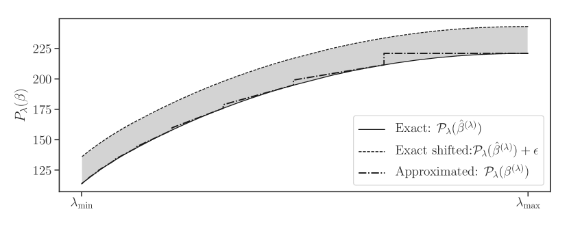
Figure 1: Illustration of the approximation path for the Lasso at accuracy $\epsilon=\left\lVert y\right\rVert_{2}^{2}/20$. We choose $\lambda_{\max}=\lVert X^{\top}y\rVert_{\infty}$ and $\lambda_{\min}=\lambda_{\max}/50$. The shaded gray region shows the interval where any $\epsilon$-path must lie. The exact path is computed with the LassoLars on diabetes data from sklearn.

In practice, obtaining $\hat{\beta}^{({\lambda})}$, an exact solution to Problem (1) is unpractical and one aims achieving a prescribed precision $\epsilon>0$. More precisely, a (primal) vector $\beta^{(\lambda)}:=\beta^{(\lambda,\epsilon)}$ (we will drop the dependency in $\epsilon$ for readability) is referred to as an $\epsilon$-solution for $\lambda$ if its (primal) objective value is optimal at precision $\epsilon$:

$$P_{\lambda}(\beta^{(\lambda)})-P_{\lambda}(\hat{\beta}^{({\lambda})})\leq\epsilon\enspace.$$ (2)

We recall and illustrate the notion of approximation path in Figure 1 as described by Giesen et al. (2012).

Definition 1 ($\epsilon$-path).

A set $\mathcal{P_{\epsilon}}\subset\mathbb{R}^{p}$ is called an $\epsilon$-path for a parameter range $[\lambda_{\min},\lambda_{\max}]$ if

$$\forall\lambda\in[\lambda_{\min},\lambda_{\max}],\exists\text{ an }\epsilon\text{-solution }\beta^{(\lambda)}\in\mathcal{P_{\epsilon}}\enspace.$$ (3)

We call path complexity $T_{\epsilon}$ the cardinality of the $\epsilon$-path.

To achieve the targeted $\epsilon$-precision in (2) over a whole path and construct an $\epsilon$-path , we rely on duality gap evaluations. For that, we compute $\epsilon_{c}$-solutions (for an accuracy $\epsilon_{c}<\epsilon$) over a finite grid, and then we control the gap variations w.r.t. $\lambda$ to achieve the prescribed $\epsilon$-precision over the whole range $[\lambda_{\min},\lambda_{\max}]$; see Algorithm 1. We now recall the Fenchel duality (Rockafellar, 1997, Chapter 31):

$$\hat{\theta}^{({\lambda})} \in\mathop{\mathrm{arg\,max}}_{\theta\in\mathbb{R}^{n}}\underbrace{-f^{*}(-\lambda\theta)-\lambda\Omega^{*}(X^{\top}\theta)}_{D_{\lambda}(\theta)}\quad\mathrm{(Dual)}.$$ (4)

For a primal/dual pair $(\beta,\theta)\in\mathrm{dom}\>P_{\lambda}\times\mathrm{dom}\>D_{\lambda}$, the duality gap is the difference between primal and dual objectives:

$$\operatorname{\mathcal{G}}_{\lambda}(\beta,\theta) =f(X\beta)+f^{*}(-\lambda\theta)+\lambda(\Omega(\beta)+\Omega^{*}(X^{\top}\theta))\enspace.$$

Weak duality yields $D_{\lambda}(\theta)\leq P_{\lambda}(\beta)$ and

$$P_{\lambda}(\beta)-P_{\lambda}(\hat{\beta}^{({\lambda})})\leq\operatorname{\mathcal{G}}_{\lambda}(\beta,\theta)\enspace,$$ (5)

explaining the interest of the duality gap as an optimality certificate. Using (5), we can safely construct an approximation path for Problem (1) : if $\beta^{(\lambda)}$ is an $\epsilon$-solution for $\lambda$, it is guaranteed to remain one for all parameters $\lambda^{\prime}$ such that $\operatorname{\mathcal{G}}_{\lambda^{\prime}}(\beta^{(\lambda)},\theta^{(\lambda)})\leq\epsilon$. Since the function $\lambda^{\prime}\mapsto\operatorname{\mathcal{G}}_{\lambda^{\prime}}(\beta^{(\lambda)},\theta^{(\lambda)})$ does not exhibit a simple dependence in $\lambda$, we rely on an upper bound on the gap encoding the structural regularity of the loss function (e.g., 1-dimensional quadratics for strongly convex functions). This bound controls the optimization error as $\lambda$ varies while preserving optimal complexity on the approximation path.

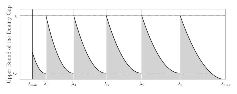
(a) Uniform unilateral approximation path (as in Proposition 3)

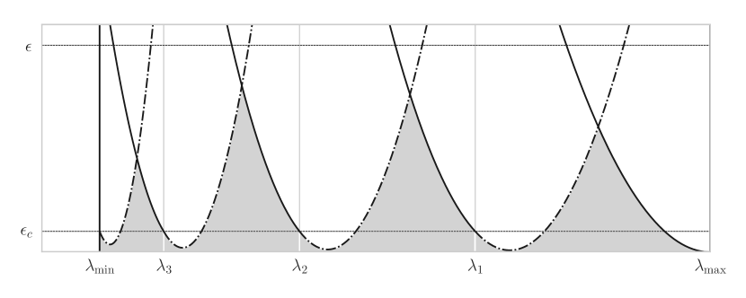
(b) Bilateral approximation path (as in Proposition 4)

Figure 2: Illustration of the construction of $\epsilon$-paths for the Lasso on synthetic dataset generated with sklearn as $X,y=$ make_regression$(n=30,p=150)$ at accuracy $\epsilon=\left\lVert y\right\rVert_{2}^{2}/40$ and $\epsilon_{c}=\epsilon/10$. We choose $\lambda_{\max}=\lVert X^{\top}y\rVert_{\infty}$ and $\lambda_{\min}=\lambda_{\max}/20$. For Lasso the bounds are piece-wise quadratic. The shaded gray regions correspond to the regions where the true value of the duality gap lies. We obtain a path complexity of $T_{\epsilon}=6$ (resp. $T_{\epsilon}=4$) for the unilateral (resp. bilateral) path over $[\lambda_{\min},\lambda_{\max}]$.

3 Bounds and approximation path

We introduce the tools to design an approximation path.

3.1 Preliminary results and technical tools

Definition 2.

Given a differentiable function $f$ and $x\in\mathrm{dom}\>f$, let $\mathcal{U}_{f,x}(\cdot)$ and $\mathcal{V}_{f,x}(\cdot)$ be non negative functions that vanish at 0. We say that $f$ is $\mathcal{U}_{f,x}$-convex (resp. $\mathcal{V}_{f,x}$-smooth) at $x$ when Inequality (6) (resp. (7)) is satisfied for any $z\in\mathrm{dom}\>f$

$$\mathcal{U}_{f,x}(z-x) \leq f(z)-f(x)-\langle\nabla f(x),z-x\rangle\enspace,$$ (6)

$$\mathcal{V}_{f,x}(z-x) \geq f(z)-f(x)-\langle\nabla f(x),z-x\rangle\enspace.$$ (7)

This extends $\mu$-strong convexity and $\nu$-smoothness (Nesterov, 2004) and encompasses smooth uniformly convex losses and generalized self-concordant ones.

Smooth uniformly convex case:

In this case, we have

$$\mathcal{U}_{f,x}(z-x)=\mathcal{U}(\lVert z-x\rVert),$$

$$\mathcal{V}_{f,x}(z-x)=\mathcal{V}(\lVert z-x\rVert),$$

where $\mathcal{U}(\cdot)$ and $\mathcal{V}(\cdot)$ are increasing from $[0,+\infty)$ to $[0,+\infty]$ vanishing at $0$; see Azé & Penot (1995). Examples of such functions are $\mathcal{U}(t)=\frac{\mu}{d}t^{d}$ and $\mathcal{V}(t)=\frac{\nu}{d}t^{d}$ where $d$, $\mu$ and $\nu$ are positive constants. The case $d=2$ corresponds to strong convexity and smoothness; in general they are called uniformly convex of order $d$, see (Juditski & Nesterov, 2014) or (Bauschke & Combettes, 2011, Ch. 10.2 and 18.5) for details.

Generalized self-concordant case:

a $\mathcal{C}^{3}$ convex function $f$ is $(M_{f},\nu)$-generalized self-concordant of order $\nu\geq 2$ and $M_{f}\geq 0$ if $\forall x\in\mathrm{dom}\>f$ and $\forall u,v\in\mathbb{R}^{n}$:

$$\left|\langle\nabla^{3}f(x)[v]u,u\rangle\right|\leq M_{f}\left\lVert u\right\rVert_{x}^{2}\left\lVert v\right\rVert_{x}^{\nu-2}\left\lVert v\right\rVert_{2}^{3-\nu}.$$

In this case, Sun & Tran-Dinh (2017, Proposition 10) have shown that one could write:

$$\mathcal{U}_{f,x}(y-x) =w_{\nu}(-d_{\nu}(x,y))\left\lVert y-x\right\rVert_{x}^{2}\enspace,$$

$$\mathcal{V}_{f,x}(y-x) =w_{\nu}(d_{\nu}(x,y))\left\lVert y-x\right\rVert_{x}^{2}\enspace,$$

where the last equality holds if $d_{\nu}(x,y)<1$ for the case $\nu>2$. Closed-form expressions of $w_{\nu}(\cdot)$ and $d_{\nu}(\cdot)$ are recalled in Appendix for logistic, quadratic and power losses.

Approximating the duality gap path.

Assume we have constructed primal/dual feasible vectors for a finite grid of parameters $\Lambda_{T}=\{\lambda_{0},\dots,\lambda_{T-1}\}$, i.e., we have at our disposal $(\beta^{(\lambda_{t})},\theta^{(\lambda_{t})})$ for all $\lambda_{t}\in\Lambda_{T}$. Let us denote $\operatorname{\mathcal{G}}_{t}=\operatorname{\mathcal{G}}_{\lambda_{t}}(\beta^{(\lambda_{t})},\theta^{(\lambda_{t})})$, and for $\zeta_{t}=-\lambda_{t}\theta^{(\lambda_{t})}$, $\Delta_{t}=f(X\beta^{(\lambda_{t})})-f(\nabla f^{*}(\zeta_{t}))$. For any function $\phi:\mathbb{R}^{n}\to[0,+\infty]$ that vanishes at $0$, $\rho\in\mathbb{R}$, we define

$$Q_{t,\phi}(\rho)=\operatorname{\mathcal{G}}_{t}+\rho\cdot(\Delta_{t}-\operatorname{\mathcal{G}}_{t})+\phi(-\rho\cdot\zeta_{t})\enspace.$$ (8)

The terms $\operatorname{\mathcal{G}}_{t}$ and $\Delta_{t}$ represent a measure of the optimization error at $\lambda_{t}$. The notation introduced in (8) will be convenient to write concisely upper and lower bounds on the duality gap. This is the goal of the next lemma which leverages regularity of the loss function $f$, as introduced in Definition 2. This provides control on how the duality gap deviates when one evaluates it for another (close) parameter $\lambda$.

Lemma 1.

We assume that $-\lambda\theta^{(\lambda_{t})}\in\mathrm{dom}\>f^{*}$ and $X^{\top}\theta^{(\lambda_{t})}\in\mathrm{dom}\>\Omega^{*}$. If $f^{*}$ is $\mathcal{V}_{f^{*}}$-smooth (resp. $\mathcal{U}_{f^{*}}$-convex), then for $\rho=1-{\lambda}/{\lambda_{t}}$, the right (resp. left) hand side of Inequality (9) holds true

$$Q_{t,\mathcal{U}_{f^{*}}}(\rho)\leq\operatorname{\mathcal{G}}_{\lambda}(\beta^{(\lambda_{t})},\theta^{(\lambda_{t})})\leq Q_{t,\mathcal{V}_{f^{*}}}(\rho)\enspace.$$ (9)

Proof.

Proof for this result and for other propositions and theorems are deferred to the Appendix. ∎

The function $\phi$, chosen as $\mathcal{V}_{f^{*}}$ (resp. $\mathcal{U}_{f^{*}}$) for the upper (resp. lower) bound, essentially captures the regularity needed to approximate the duality gap at $\lambda$ when using primal/dual vector $(\beta^{(\lambda_{t})},\theta^{(\lambda_{t})})$ for $\lambda_{t}$ close to $\lambda$. When the function satisfies both inequalities, tightness of the bounds can be related to the conditioning $\mathcal{U}_{f^{*}}/\mathcal{V}_{f^{*}}$ of the dual loss $f^{*}$. Equality holds for $\mathcal{U}_{f^{*}}\equiv\mathcal{V}_{f^{*}}\equiv\tfrac{1}{2}{\left\lVert\cdot\right\rVert_{2}^{2}}$ (least-squares), showing the tightness of the bounds.

From Lemma 1, we have $\operatorname{\mathcal{G}}_{\lambda}(\beta^{(\lambda_{t})},\theta^{(\lambda_{t})})\leq\epsilon$ as soon as $Q_{t,\mathcal{V}_{f^{*}}}(\rho)\leq\epsilon$ where $\rho=1-\lambda/\lambda_{t}$ varies with $\lambda$. Hence, we obtain the following proposition that allows to track the regularization path for an arbitrary precision on the duality gap. It proceeds by choosing the largest $\rho=\rho_{t}$ such that the upper bound in Equation 9 remains below $\epsilon$ and leads to Algorithm 1 for computing an $\epsilon$-path.

Proposition 1 (Grid for a prescribed precision).

 
Given $(\beta^{(\lambda_{t})},\theta^{(\lambda_{t})})$ such that $\operatorname{\mathcal{G}}_{t}\leq\epsilon_{c}<\epsilon$, for all $\lambda\in\lambda_{t}\times\left[1-\rho_{t}^{\ell}(\epsilon),\,1+\rho_{t}^{r}(\epsilon)\right]$, we have $\operatorname{\mathcal{G}}_{\lambda}(\beta^{(\lambda_{t})},\theta^{(\lambda_{t})})\leq\epsilon$ where $\rho_{t}^{\ell}(\epsilon)$ (resp. $\rho_{t}^{r}(\epsilon)$) is the largest non-negative $\rho$ s.t. $Q_{t,\mathcal{V}_{f^{*}}}(\rho)\leq\epsilon$ (resp. $Q_{t,\mathcal{V}_{f^{*}}}(-\rho)\leq\epsilon$).

Conversely, given a grid of $T$ parameters $\Lambda_{T}=\{\lambda_{0},\dots,\lambda_{T-1}\}$, we define $\epsilon_{\Lambda_{T}}$, the error of the approximation path on $[\lambda_{\min},\lambda_{\max}]$ by using a piecewise constant approximation of the map $\lambda\mapsto\operatorname{\mathcal{G}}_{\lambda}(\beta^{(\lambda_{t})},\theta^{(\lambda_{t})})$:

$$\epsilon_{\Lambda_{T}}:=\max_{\lambda\in[\lambda_{\min},\lambda_{\max}]}\min_{\lambda_{t}\in\Lambda_{T}}\operatorname{\mathcal{G}}_{\lambda}(\beta^{(\lambda_{t})},\theta^{(\lambda_{t})})\enspace.$$ (10)

This error is however difficult to evaluate in practice so we rely on a tight upper bound based on Lemma 1 that often leads to closed-form expressions.

Proposition 2 (Precision for a given grid).

Given a grid of parameters $\Lambda_{T}$, the set $\{\beta^{(\lambda)}:\lambda\in\Lambda_{T}\}$ is an $\epsilon_{\Lambda_{T}}$-path with $\epsilon_{\Lambda_{T}}\leq\max_{t\in[T]}Q_{t,\mathcal{V}_{f^{*}}}(1-\lambda_{t}^{\star}/\lambda_{t})$ where for all $t\in\{0,\dots,T-1\}$, $\lambda_{t}^{\star}$ is the largest $\lambda\in[\lambda_{t+1},\lambda_{t}]$ such that $Q_{t,\mathcal{V}_{f^{*}}}(1-\lambda/\lambda_{t})\geq Q_{t+1,\mathcal{V}_{f^{*}}}(1-\lambda/\lambda_{t+1})$.

Construction of dual feasible vector.

We rely on gradient rescaling to produce a dual feasible vector:

Lemma 2.

For any $\beta^{(\lambda_{t})}\in\mathbb{R}^{p}$, the vector

$$\theta^{(\lambda_{t})}=\frac{-\nabla f(X\beta^{(\lambda_{t})})}{\max(\lambda_{t},\sigma_{\mathrm{dom}\>\Omega^{*}}^{\circ}(X^{\top}\nabla f(X\beta^{(\lambda_{t})}))}\enspace,$$

is feasible: $-\lambda\theta^{(\lambda_{t})}\in\mathrm{dom}\>f^{*}$, $X^{\top}\theta^{(\lambda_{t})}\in\mathrm{dom}\>\Omega^{*}$.

Remark 1.

When the regularization is a norm, $\Omega(\cdot)=\left\lVert\cdot\right\rVert$ then $\sigma_{\mathrm{dom}\>\Omega^{*}}^{\circ}$ is the associated dual norm $\left\lVert\cdot\right\rVert_{*}$.

The dual $\theta^{(\lambda_{t})}$ in Lemma 2 implies that $\operatorname{\mathcal{G}}_{t}$ and $\Delta_{t}$ converge to $0$ when $\beta^{(\lambda_{t})}$ converges to $\hat{\beta}^{(\lambda_{t})}$ (Ndiaye et al., 2017).

Finding $\rho$.

Following Proposition 1, a 1-dimensional equation $Q_{t,\mathcal{V}_{f^{*}}}(\rho)=\epsilon$ needs to be solved to obtain an $\epsilon$-path. This can be done efficiently at high precision by numerical solvers if no explicit solution is available.

As a corollary from Lemma 1 and Proposition 2, we recover the analysis by Giesen et al. (2012):

Corollary 1.

If the function $f^{*}$ is $\frac{\nu}{2}\lVert\cdot\rVert^{2}$-smooth, the left ($\rho^{\ell}_{t}$) and right ($\rho^{r}_{t}$) step sizes defined in Proposition 1 have closed-form expressions:

$$\rho^{\ell}_{t}=\frac{\!\sqrt{\!2\nu\delta_{t}\left\lVert\zeta_{t}\right\rVert^{2}\!+{\tilde{\delta}_{t}}^{2}}-\tilde{\delta}_{t}}{\nu\left\lVert\zeta_{t}\right\rVert^{2}},\rho^{r}_{t} =\frac{\!\sqrt{\!2\nu\delta_{t}\left\lVert\zeta_{t}\right\rVert^{2}\!+{\tilde{\delta}_{t}}^{2}}+\tilde{\delta}_{t}}{\nu\left\lVert\zeta_{t}\right\rVert^{2}},$$

where $\delta_{t}:=\epsilon-\operatorname{\mathcal{G}}_{t}$ and $\tilde{\delta}_{t}:=\Delta_{t}-\operatorname{\mathcal{G}}_{t}$. This is simplified to $\delta_{t}=\epsilon-\epsilon_{c}$ and $\tilde{\delta}_{t}=0$ when $\max(\operatorname{\mathcal{G}}_{t},\Delta_{t})\leq\epsilon_{c}$.

Algorithm 1 training_path

  Input: $f,\Omega,\epsilon,\epsilon_{c},[\lambda_{\min},\lambda_{\max}]$

  Initialization: $t=0$, $\lambda_{0}=\lambda_{\max}$, $\Lambda=\{\lambda_{\max}\}$

  repeat

     Get $\beta^{(\lambda_{t})}$ solving (1) to accuracy $\operatorname{\mathcal{G}}_{t}\leq\epsilon_{c}<\epsilon$

     Compute the step size $\rho_{t}^{\ell}(\epsilon)$ following Proposition 3, 4, 5.

     Set $\lambda_{t+1}=\max(\lambda_{t}\times(1-\rho_{t}^{\ell}),\,\lambda_{\min})$

     $\Lambda\leftarrow\Lambda\cup\{\lambda_{t+1}\}$ and $t\leftarrow t+1$

  until $\lambda_{t}\leq\lambda_{\min}$

  Return: $\{\beta^{(\lambda_{t})}\;:\;\lambda_{t}\in\Lambda\}$

3.2 Discretization strategies

We now establish new strategies for the exploration of the hyperparameter space in the search for an $\epsilon$-path.

For regularized learning methods, it is customary to start from a large regularizer $\lambda_{0}=\lambda_{\max}$ and then to perform the computation of $\hat{\beta}^{({\lambda_{t+1}})}$ after the one of $\hat{\beta}^{({\lambda_{t}})}$, until the smallest parameter of interest $\lambda_{\min}$ is reached. Models are generally computed by increasing complexity, allowing important speed-ups due to warm start (Friedman et al., 2007) when the $\lambda$’s are close to each other. Knowing $\lambda_{t}$, we provide a recursive strategy to construct $\lambda_{t+1}$.

Adaptive unilateral.

The strategy we call unilateral consists in computing the new parameter as $\lambda_{t+1}=\lambda_{t}\times(1-\rho_{t}^{\ell}(\epsilon))$ as in Proposition 1.

Proposition 3 (Unilateral approximation path).

Assume that $f^{*}$ is $\mathcal{V}_{f^{*}}$-smooth. We construct the grid of parameters $\Lambda^{(u)}(\epsilon)=\{\lambda_{0},\ldots,\lambda_{T_{\epsilon}-1}\}$ by

$$\lambda_{0}=\lambda_{\max},\quad\lambda_{t+1}=\lambda_{t}\times(1-\rho_{t}^{\ell}(\epsilon))\enspace,$$

and $(\beta^{(\lambda_{t})},\theta^{(\lambda_{t})})$ s.t. $\operatorname{\mathcal{G}}_{t}\leq\epsilon_{c}<\epsilon$ for all $t$. Then, the set $\{\beta^{(\lambda_{t})}\;:\;\lambda_{t}\in\Lambda^{(u)}(\epsilon)\}$ is an $\epsilon$-path for Problem (1).

This strategy is illustrated in 2(a) on a Lasso case, and stands as a generic one to compute an approximation path for loss functions satisfying assumptions in Definition 2.

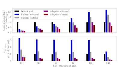
(a) $\ell_{1}$ least-squares regression on climate data set NCEP/NCAR Reanalysis; $n=814$ observations and $p=73577$ features.

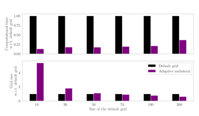
(b) $\ell_{1}$ logistic regression on leukemia data set with $n=72$ observations and $p=7129$ features.

Figure 3: Computation of the approximation path to reach the same error than the default grid ($\epsilon=10^{-4}\left\lVert y\right\rVert^{2}$ for the least-squares case and $\epsilon=10^{-4}\min(n_{1},n_{2})/n$ where $n_{i}$ is the number of observations in the class $i\in\{0,1\}$, for the logistic case). We have used the same (vanilla) coordinate descent optimization solver with warm start between parameters for all grids. Note that a smaller grid do not imply faster computation, as the interplay with the warm-start can be intricate in our sequential approach.

Adaptive bilateral.

For uniformly convex functions, we can make a larger step by combining the information given by the left and right step sizes. Indeed, let us assume that we explore the parameter range $[\lambda_{\min},\lambda_{\max}]$. Starting from a parameter $\lambda_{t}$, we define the next step, given by Proposition 1, $\lambda_{t}^{\ell}:=\lambda_{t}(1-\rho_{t}^{\ell})$. Then it exists $\lambda_{t^{\prime}}\leq\lambda_{t}^{\ell}$ such that $\lambda_{t^{\prime}}^{r}:=\lambda_{t^{\prime}}(1+\rho_{t^{\prime}}^{r})=\lambda_{t}^{\ell}$. Thus a larger step can be done by using $\lambda_{t^{\prime}}=\lambda_{t}\times{(1-\rho_{t}^{\ell})}/{(1+\rho_{t^{\prime}}^{r})}$. However $\rho_{t^{\prime}}^{r}$ depends on the (approximated) solution $\beta^{(\lambda_{t^{\prime}})}$ that we do not know before optimizing the problem for parameter $\lambda_{t^{\prime}}$ when computing sequentially the grid points in decreasing order i.e., $\lambda_{t^{\prime}}\leq\lambda_{t}$. We overcome this issue in Lemma 3 by (upper) bounding all the constants in $Q_{t^{\prime},\mathcal{V}_{f^{*}}}(\rho)$ that depend on the solution $\beta^{(\lambda_{t^{\prime}})}$, by constants involving only information given by $\beta^{(\lambda_{t})}$.

Lemma 3.

Assuming $f$ uniformly smooth yields $\lVert\nabla f(X\beta^{(\lambda_{t^{\prime}})})\rVert_{*}\leq\widetilde{R}_{t}$, where $\widetilde{R}_{t}:={\mathcal{V}_{f}^{*}}^{-1}\big{(}f(X\beta^{(\lambda_{t})})+\frac{2\epsilon_{c}}{\rho_{t}^{\ell}(\epsilon)}\big{)}$. If additionally $f$ is uniformly convex, this yields $\Delta_{t^{\prime}}\leq\widetilde{\Delta}_{t}$, where $\widetilde{\Delta}_{t}:=\widetilde{R}_{t}\times\mathcal{U}_{f}^{-1}(\epsilon_{c})$ as well as $\operatorname{\mathcal{G}}_{\lambda}(\beta^{(\lambda_{t^{\prime}})},\theta^{(\lambda_{t^{\prime}})})\leq Q_{t^{\prime},\mathcal{V}_{f^{*}}}(\rho)\leq\widetilde{Q}_{t,\mathcal{V}_{f^{*}}}(\rho)$, where

$$\widetilde{Q}_{t,\mathcal{V}_{f^{*}}}(\rho)=\epsilon_{c}+\rho\cdot(\widetilde{\Delta}_{t}-\epsilon_{c})+\mathcal{V}_{f^{*}}\left(\left|\rho\right|\cdot\widetilde{R}_{t}\right)\enspace.$$

Let us now define $\rho_{t}^{(b)}(\epsilon)=\displaystyle\frac{\rho_{t}^{\ell}(\epsilon)+\tilde{\rho}_{t}^{r}(\epsilon)}{1+\tilde{\rho}_{t}^{r}(\epsilon)}$, where $\rho_{t}^{\ell}(\epsilon)$ is defined in Proposition 1 and $\tilde{\rho}_{t}^{r}(\epsilon)$ is the largest non negative $\rho$ such that $\widetilde{Q}_{t,\mathcal{V}_{f^{*}}}(\rho)\leq\epsilon$ in Lemma 3.

Proposition 4 (Bilateral Approximation Path).

Assume that $f$ is uniformly convex and smooth. We construct the grid $\Lambda^{(b)}(\epsilon)=\{\lambda_{0},\ldots,\lambda_{T_{\epsilon}-1}\}$ by

$$\lambda_{0}=\lambda_{\max},\quad\lambda_{t+1}=\lambda_{t}\times(1-\rho_{t}^{(b)}(\epsilon))\enspace,$$

and $(\beta^{(\lambda_{t})},\theta^{(\lambda_{t})})$ s.t. $\operatorname{\mathcal{G}}_{t}\leq\epsilon_{c}<\epsilon$ for all $t$. Then the set $\{\beta^{(\lambda_{t})}\;:\;\lambda_{t}\in\Lambda^{(b)}(\epsilon)\}$ is an $\epsilon$-path for Problem (1).

This strategy is illustrated in 2(b) on a Lasso example.

Uniform unilateral and bilateral.

In some cases, it may be advantageous to have access to a predefined grid before launching a hyperparameter selection procedure such as hyperband (Li et al., 2017) or for parallel computations. Given the initial information from the initialization $(\beta^{(\lambda_{0})},\theta^{(\lambda_{0})})$, we can build a uniform grid that guarantees an $\epsilon$-approximation before solving any optimization problem. Indeed, by applying Lemma 3 at $t=0$, we have $\operatorname{\mathcal{G}}_{\lambda}(\beta^{(\lambda_{t})},\theta^{(\lambda_{t})})\leq\widetilde{Q}_{0,\mathcal{V}_{f^{*}}}(\rho)$. We can define $\widetilde{\rho}_{0}^{\ell}(\epsilon)$ (resp. $\widetilde{\rho}_{0}^{r}(\epsilon)$) as the largest non-negative $\rho$ s.t. $\widetilde{Q}_{0,\mathcal{V}_{f^{*}}}(\rho)\leq\epsilon$ (resp. $\widetilde{Q}_{0,\mathcal{V}_{f^{*}}}(-\rho)\leq\epsilon$) and also

$$\rho_{0}(\epsilon)=\begin{cases}\widetilde{\rho}_{0}^{\ell}(\epsilon)&\text{for \emph{unilateral} path},\\ \frac{\widetilde{\rho}_{0}^{\ell}(\epsilon)+\widetilde{\rho}_{0}^{r}(\epsilon)}{1+\tilde{\rho}_{0}^{r}(\epsilon)}&\text{for \emph{bilateral} path}.\end{cases}$$ (11)

Proposition 5 (Uniform approximation path).

 
Assume that $f$ is uniformly convex and smooth, and define the grid $\Lambda^{(0)}(\epsilon)=\{\lambda_{0},\ldots,\lambda_{T_{\epsilon}-1}\}$ by

$$\lambda_{0}=\lambda_{\max},\quad\lambda_{t+1}=\lambda_{t}\times(1-\rho_{0}(\epsilon))\enspace,$$

and $\forall t\in[T],(\beta^{(\lambda_{t})},\theta^{(\lambda_{t})})$ s.t. $\operatorname{\mathcal{G}}_{t}\leq\epsilon_{c}<\epsilon$. Then the set $\{\beta^{(\lambda_{t})}\;:\;\lambda_{t}\in\Lambda^{(0)}(\epsilon)\}$ is an $\epsilon$-path for Problem (1) with at most $T_{\epsilon}$ grid points where

$$T_{\epsilon}=\left\lfloor\frac{\log({\lambda_{\min}}/{\lambda_{\max}})}{\log(1-\rho_{0}(\epsilon))}\right\rfloor\enspace.$$ (12)

3.3 Limitations of previous framework

Previous algorithms for computing $\epsilon$-paths have been initially developed with a complexity of $O(1/\epsilon)$ (Clarkson, 2010; Giesen et al., 2010) in a large class of problems. Yet, losses arising in machine learning have often nicer regularities that can be exploited. This is all the more striking in the Lasso case where a better complexity in $O(1/\sqrt{\epsilon})$ was obtained by Mairal & Yu (2012); Giesen et al. (2012).

The relation between path complexity and regularity of the objective function remains unclear and previous methods do not apply to all popular learning problems. For instance the dual loss $f^{*}$ of the logistic regression is not uniformly smooth. So to apply the previous theory, one needs to optimize on a (potentially badly pre-selected) compact set.

Let us consider the one dimensional toy example where $p=1$, $\beta\in\mathbb{R}$, $X=\mathrm{Id}_{p}$, $y=-1$ and the loss function $f(X\beta)=\log(1+\exp(\beta))$. We have, $\nabla^{2}f(\beta)=\exp(\beta)/(1+\exp(\beta))^{2}$. Then for Problem (1), since $P_{\lambda}(\hat{\beta}^{({\lambda})})\leq P_{\lambda}(0)$, we have $|\hat{\beta}^{({\lambda})}|\in[0,\log(2)/\lambda]$ and a smoothness constant $\nu_{f^{*}}\approx\exp(\lambda)$ for the dual can be estimated at each step. This leads to an unreasonable algorithm with tiny step sizes in Corollary 1. Also, the algorithm proposed by Giesen et al. (2012) can not be applied for the logistic loss since the dual function is not polynomial.

Our proposed algorithm does not suffer from such limitations and we introduce a finer analysis that takes into account the regularity of the loss functions.

3.4 Complexity and regularity

Lower bound on path complexity.

For our method, the lower bound on the duality gap quantifies how close the from Proposition 1 is from the best possible one can achieve for smooth loss functions. Indeed, at optimal solution, we have $\operatorname{\mathcal{G}}_{t}=\Delta_{t}=0$. Thus the largest possible step — starting at $\lambda_{t}$ and moving in decreasing order — is given by the smallest $\lambda\in[\lambda_{\min},\lambda_{t}]$ such that $\mathcal{U}_{f^{*}}(-\hat{\zeta}_{t}\times\rho)>\epsilon$ where $\hat{\zeta}_{t}=-\lambda_{t}\hat{\theta}^{({\lambda_{t}})}$. Hence, any algorithm for computing an $\epsilon$-path for $\mathcal{U}_{f^{*}}$-uniformly convex dual loss, have necessarily a complexity of order at least $O(1/\mathcal{U}_{f^{*}}^{-1}(\epsilon))$.

Upper bounds.

We remind that we write $T_{\epsilon}$ for the complexity of our proposed approximation path i.e., the cardinality of the grid returned by Algorithm 1. In the following proposition, we propose a bound on the complexity w.r.t. the regularity of the loss function. Discussions on the constants and assumptions are provided in the Appendix.

Proposition 6 (Approximation path: complexity).

Assuming that $\max(\operatorname{\mathcal{G}}_{t},\Delta_{t})\leq\epsilon_{c}<\epsilon$ at each step $t$, there exists an explicit constant $C_{f}(\epsilon_{c})>0$ such that

$$T_{\epsilon} \leq\log\Big{(}\frac{\lambda_{\max}}{\lambda_{\min}}\Big{)}\times\frac{C_{f}(\epsilon_{c})}{\mathcal{W}_{f^{*}}(\epsilon-\epsilon_{c})}\enspace,$$ (13)

where for all $t>0$, the function $\mathcal{W}_{f^{*}}$ is defined by

$$\mathcal{W}_{f^{*}}(\cdot)=\begin{cases}\mathcal{V}_{f^{*}}^{-1}(\cdot),&\!\!\!\text{if }f\text{ is uniformly convex and smooth}\\ \sqrt{\cdot},&\!\!\!\text{if }f\text{ is Generalized Self-Concordant}\\ &\text{and uniformly-smooth.}\end{cases}$$

Moreover, $C_{f}(\epsilon_{c})$ is an uniform upper bound of $\left\lVert\zeta_{t}\right\rVert_{*}$ along the path, that tends to a constant $C_{f}$ when $\epsilon_{c}$ goes to $0$.

Proposition 6 applied to the special case when $f$ is $\nu$-smooth and $\mu$-strongly convex reads $\log\Big{(}\frac{\lambda_{\max}}{\lambda_{\min}}\Big{)}\sqrt{\frac{\nu}{\mu}\frac{f(X\beta^{(\lambda_{0})})}{\epsilon-\epsilon_{c}}}$ for the complexity for any data $X,y$. This is not explicitly dependent on the dimension $n$ and $p$ and are more scalable.

4 Validation path

Algorithm 2 $\epsilon_{v}$-path for Validation Set

  Input: $f,\Omega,\epsilon_{v},[\lambda_{\min},\lambda_{\max}]$

  Compute $\epsilon_{v,\mu}$ as in Proposition 7

  $\Lambda(\epsilon_{v,\mu})=\texttt{training\_path}\left(f,\Omega,\epsilon_{v,\mu},[\lambda_{\min},\lambda_{\max}]\right)$

  Return: $\Lambda(\epsilon_{v,\mu})$

To achieve good generalization performance, estimators defined as solutions of Problem 1 require a careful adjustment of $\lambda$ to balance data-fitting and regularization. A standard approach to calibrate such a parameter is to select it by comparing the validation errors on a finite grid (say with K-fold cross-validation). Unfortunately, it is often difficult to determine a priori the grid limits, the number of $\lambda$’s (number of points in the grid) or how they should be distributed to achieve low validation error.

Considering the validation data $({X^{\prime}},{y^{\prime}})$ with $n^{\prime}$ observations and loss $\mathcal{L}$, we define the validation error for $\beta\in\mathbb{R}^{p}$:

$$E_{v}(\beta)=\mathcal{L}({y^{\prime}},{X^{\prime}}\beta)\enspace.$$ (14)

For selecting a hyperparameter, we leverage our approximation path to solve the bi-level problem

$$\mathop{\mathrm{arg\,min}}_{\lambda\in[\lambda_{\min},\lambda_{\max}]} E_{v}(\hat{\beta}^{({\lambda})})=\mathcal{L}(y^{\prime},X^{\prime}\hat{\beta}^{({\lambda})})$$

$$\text{s.t. }\hat{\beta}^{({\lambda})}\in\mathop{\mathrm{arg\,min}}_{\beta\in\mathbb{R}^{p}}f(X\beta)+\lambda\Omega(\beta)\enspace.$$

Recent works have addressed this problem by using gradient-based algorithms, see for instance Pedregosa (2016); Franceschi et al. (2018) who have shown promising results in computational time and scalability w.r.t. multiple hyperparameters. Yet, they require assumptions such as smoothness of the validation function $E_{v}$ and non-singular Hessian of the inner optimization problem at optimal values which are difficult to check in practice since they depend on the optimal solutions $\hat{\beta}^{({\lambda})}$. Moreover, they can only guarantee convergence to stationary point.

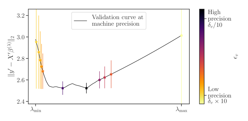
(a) Synthetic data set generated using the sklearn command $X,y=$ make_sparse_uncorrelated$(n=30,p=50)$.

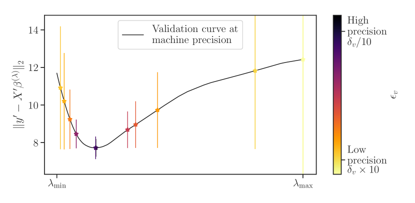
(b) Synthetic data set generated using the sklearn command $X,y=$ make_regression$(n=500,p=5000)$.

Figure 4: Safe selection of the optimal hyperparameter for Enet on the validation set (30% of the observations). The targeted accuracy $\epsilon_{v}$ is refined from $\delta_{v}\times 10$ to $\delta_{v}/10$ with $\delta_{v}=\max_{\lambda_{t}\in\Lambda}E_{v}(\beta^{(\lambda_{t})})-\min_{\lambda_{t}\in\Lambda}E_{v}(\beta^{(\lambda_{t})})$ and $\Lambda$ is the default grid between $\lambda_{\max}=\lVert X^{\top}y\rVert_{\infty}$ and $\lambda_{\min}=\lambda_{\max}/100$ of size $T=200$. The stars represent the worst case solution amount the one generated by Algorithm 2 (with bilateral path). For loose precision suboptimal parameters are identified, but better ones are found as the accuracy $\epsilon_{v}$ decreases.

In this section, we generalize the approach of (Shibagaki et al., 2015) and show that with a safe and simple exploration of the parameter space, our algorithm has a global convergence property. For that, we assume the following conditions on the validation loss and on the inner optimization objective throughout the section:

$$|\mathcal{L}(a,b)-\mathcal{L}(a,c)|\leq\mathcal{L}(b,c)\text{ for any }a,b,c\in\mathbb{R}^{n}.$$ A1

$$\text{The function }\beta\mapsto P_{\lambda}(\beta)\text{ is }\mu\text{-strongly convex}.$$ A2

The assumption on the loss function is verified for norms (regression) and indicator functions (classification). Indeed, if $\mathcal{L}(a,b)=\lVert a-b\rVert$, A1 corresponds to the triangle inequality. For the $\ell_{0/1}$-loss $\mathcal{L}(a,b)=\frac{1}{n}\sum_{i=1}^{n}\mathbf{1}_{a_{i}b_{i}<0}$, since for any real $s,u$ and $v$, $|\mathbf{1}_{us<0}-\mathbf{1}_{uv<0}|\leq\mathbf{1}_{sv<0}$, one has

$$\Big{|}\frac{1}{n}\sum_{i=1}^{n}\mathbf{1}_{a_{i}b_{i}<0}-\frac{1}{n}\sum_{i=1}^{n}\mathbf{1}_{a_{i}c_{i}<0}\Big{|}\leq\frac{1}{n}\sum_{i=1}^{n}\mathbf{1}_{b_{i}c_{i}<0}\enspace.$$

Definition 3.

Given a primal solution $\hat{\beta}^{({\lambda})}$ for parameter $\lambda$ and a primal point $\beta^{(\lambda_{t})}$ returned by an algorithm, we define the gap on the validation error between $\lambda$ and $\lambda_{t}$ as

$$\Delta E_{v}(\lambda_{t},\lambda):=\big{|}E_{v}(\hat{\beta}^{({\lambda})})-E_{v}(\beta^{(\lambda_{t})})\big{|}\enspace.$$ (15)

Suppose we have fixed a tolerance $\epsilon_{v}$ on the gap on validation error i.e., $\Delta E_{v}(\lambda_{t},\lambda)\leq\epsilon_{v}$. Based on Assumption A1, if there is a region $\mathcal{R}_{\lambda}$ that contains the optimal solution $\hat{\beta}^{({\lambda})}$ at parameter $\lambda$, then we have

$$\Delta E_{v}(\lambda_{t},\lambda) \leq\mathcal{L}({X^{\prime}}\hat{\beta}^{({\lambda})},{X^{\prime}}\beta^{(\lambda_{t})})$$

$$\leq\max_{\beta\in\mathcal{R}_{\lambda}}\mathcal{L}({X^{\prime}}\beta,{X^{\prime}}\beta^{(\lambda_{t})})\enspace.$$

A simple strategy consists in choosing $\mathcal{R}_{\lambda}$ as a ball.

Lemma 4 (Gap safe region Ndiaye et al. (2017)).

Under A2, any primal solution $\hat{\beta}^{({\lambda})}$ belongs to the Euclidean ball with center $\beta^{(\lambda_{t})}$ and radius

$$r_{t,\mu}(\lambda)=\sqrt{\frac{2}{\mu}\operatorname{\mathcal{G}}_{\lambda}(\beta^{(\lambda_{t})},\theta^{(\lambda_{t})})}\enspace.$$ (16)

Such a safe ball leveraging duality gap has been proved useful to speed-up sparse optimization solvers. The improve performance relies on the ability to identify the sparsity structure of the optimal solutions; approaches of this type are referred to as safe screening rules as they provide safe certificates for such structures (El Ghaoui et al., 2012; Fercoq et al., 2015; Shibagaki et al., 2016; Ndiaye et al., 2017).

Since the radius in Equation 16 depends explicitly on the duality gap, we can sequentially track a range of parameters for which the gap on the validation error remains below a prescribed tolerance by controlling the optimization error.

Proposition 7 (Grid for prescribed validation error).

Under Assumptions A1 and A2, let us define for $i\in[n^{\prime}]$ an index in the test set, $\xi_{i}=\left(\tfrac{{x^{\prime}}_{\!\!i}^{\top}\beta^{(\lambda_{t})}}{\left\lVert{x^{\prime}}_{\!\!i}\right\rVert}\right)^{2}$ and

$$\epsilon_{v,\mu}=\begin{cases}\frac{\mu}{2}\times\left(\frac{\epsilon_{v}}{\lVert X^{\prime}\rVert}\right)^{2},&\text{(regression)}\\ \frac{\mu}{2}\times\xi_{(\lfloor n\epsilon_{v}\rfloor+1)},&\text{(classification)}\end{cases}$$ (17)

where $\xi_{(\lfloor n\epsilon_{v}\rfloor+1)}$ is the $(\lfloor n\epsilon_{v}\rfloor+1)$-th smallest value of $\xi_{i}$’s. Given $(\beta^{(\lambda_{t})},\theta^{(\lambda_{t})})$ such that $\operatorname{\mathcal{G}}_{t}\leq\epsilon_{v,\mu}$, we have $\Delta E_{v}(\lambda_{t},\lambda)\leq\epsilon_{v}$ for all parameter $\lambda$ in the interval
$\lambda_{t}\times\left[1-\rho_{t}^{\ell}(\epsilon_{v,\mu}),\,1+\rho_{t}^{r}(\epsilon_{v,\mu})\right],$ where $\rho_{t}^{\ell}(\epsilon_{v,\mu})$, $\rho_{t}^{r}(\epsilon_{v,\mu})$ are defined in Proposition 1.

Remark 2 (Stopping criterion for training).

For the current parameter $\lambda_{t}$, $\Delta E_{v}(\lambda_{t},\lambda_{t})\leq\epsilon_{v}$ as soon as $\operatorname{\mathcal{G}}_{t}\leq\epsilon_{v,\mu}$, which gives us a stopping criterion for optimizing on the training part $(X,y)$ relative to the desired accuracy $\epsilon_{v}$ on the validation data $(X^{\prime},y^{\prime})$. This has the appealing property of relieving the practitioner from selecting the stopping criterion $\epsilon_{c}$ when optimizing on the training set.

Algorithm 2 outputs a discrete set of parameters $\Lambda(\epsilon_{v,\mu})$ such that $\{\beta^{(\lambda_{t})}\text{ for }\lambda_{t}\in\Lambda(\epsilon_{v,\mu})\}$ is an $\epsilon_{v}$-path for the validation error. Thus, for any $\lambda\in[\lambda_{\min},\lambda_{\max}]$, there exists $\lambda_{t}\in\Lambda(\epsilon_{v,\mu})$ such that

$$E_{v}(\beta^{(\lambda_{t})})-\epsilon_{v}\leq E_{v}(\hat{\beta}^{({\lambda})})\enspace.$$ (18)

The following proposition is obtained by taking the minimum on both sides of the inequality.

Proposition 8.

Under Assumptions A1 and A2, the set $\{\beta^{(\lambda_{t})}\text{ for }\lambda_{t}\in\Lambda(\epsilon_{v,\mu})\}$ is an $\epsilon_{v}$-path for the error and

$$\min_{\lambda_{t}\in\Lambda(\epsilon_{v,\mu})}E_{v}(\beta^{(\lambda_{t})})-\min_{\lambda\in[\lambda_{\min},\lambda_{\max}]}E_{v}(\hat{\beta}^{({\lambda})})\leq\epsilon_{v}\enspace.$$

5 Numerical experiments

We illustrate our method on $\ell_{1}$-regularized least squares and logistic regression by comparing the computational times and number of grid points needed to compute an $\epsilon$-path for a given range $[\lambda_{\min},\lambda_{\max}]$ for several strategies.

The ”Default grid” is the one used by default in the packages glmnet (Friedman et al., 2010) and sklearn (Pedregosa et al., 2011). It is defined as $\lambda_{t}=\lambda_{\max}\times 10^{-\delta t/(T-1)}$ (here $\delta=3$). The proposed grids are the adaptive unilateral/bilateral and uniform unilateral/bilateral grids that are defined in Propositions 3, 4 and 5.

Thanks to Proposition 2, we measure the approximation path error $\epsilon$ of the default grid of size $T$ and report the times and numbers of grid points $T_{\epsilon}$ needed to achieve such a precision. Our experiments were conducted on the leukemia dataset, available in sklearn and the climate dataset NCEP/NCAR Reanalysis (Kalnay et al., 1996). The optimization algorithms are the same for all the grid, hence we compare only the grid construction impact. Results are reported in Figure 3 for classification and regression problem. Our approach leads to better guarantees for approximating the regularization path w.r.t. the default grid and often significant gain in computing time.

Figure 4 illustrates convergence for Elastic Net (Enet) (Zou & Hastie, 2005), on synthetic data generated by sklearn as random regression problems make_regression and make_sparse_uncorrelated (Celeux et al., 2012). For a decreasing levels of validation error, we represent the $\lambda$ selected by our algorithm and its corresponding safe interval. Even when the validation curve is non smooth and non convex, the output of the safe grid search converges to the global minimum as stated in Proposition 8.

6 Conclusion

We have shown how to efficiently construct one dimensional grids of regularization parameters for convex risk minimization, and to get an automatic calibration, optimal in term of hold-out test error. Future research could examine how to adapt our framework to address multi-dimensional parameter grids. This case is all the more interesting that it naturally arises when addressing non-convex problems, e.g., MCP or SCAD, with re-weighted $\ell_{1}$-minimization. Approximation of a full path then requires to optimize up to precision $\epsilon_{c}$ at each step, even for non promising hyperparameter, which is time consuming. Combining our approach with safe elimination procedures could provide faster hyperparameter selection algorithms.

7 Appendix

7.1 Generalized self-concordant functions

Proposition 9 (Sun & Tran-Dinh (2017), Proposition 10).

If $(M_{f},\nu)$-generalized self concordant, then

$$w_{\nu}(-d_{\nu}(x,y))\left\lVert y-x\right\rVert_{x}^{2}\leq f(y)-f(x)-\langle\nabla f(x),y-x\rangle\leq w_{\nu}(d_{\nu}(x,y))\left\lVert y-x\right\rVert_{x}^{2}\enspace,$$ (19)

where the right-hand side inequality holds if $d_{\nu}(x,y)<1$ for the case $\nu>2$ and where

$$d_{\nu}(x,y):=\begin{cases}M_{f}\left\lVert y-x\right\rVert_{2}&\text{ if }\nu=2,\\ \left(\frac{\nu}{2}-1\right)M_{f}\left\lVert y-x\right\rVert_{2}^{3-\nu}\left\lVert y-x\right\rVert_{x}^{\nu-2}&\text{ if }\nu>2,\end{cases}$$ (20)

and

$$w_{\nu}(\tau):=\begin{cases}\frac{e^{\tau}-\tau-1}{\tau^{2}}&\text{ if }\nu=2,\\ \frac{-\tau-\log(1-\tau)}{\tau^{2}}&\text{ if }\nu=3,\\ \frac{(1-\tau)\log(1-\tau)+\tau}{\tau^{2}}&\text{ if }\nu=4,\\ \left(\frac{\nu-2}{4-\nu}\right)\frac{1}{\tau}\left[\frac{\nu-2}{2(3-\nu)\tau}\left((1-\tau)^{\frac{2(3-\nu)}{2-\nu}}-1\right)-1\right]&\text{ otherwise.}\end{cases}$$ (21)

The dual of the logistic loss is Generalized Self-Concordant with $M_{f^{*}}=1,\nu=4$. Power loss function $f_{i}(z)=(y_{i}-z)^{q}$ for $q\in(1,2)$, popular in robust regression, is covered with $M_{f}=\frac{2-q}{\sqrt[(2-q)]{q(q-1)}},\nu=\frac{2(3-q)}{2-q}$. We refer to (Sun & Tran-Dinh, 2017) for more details and examples.

Remark 3.

Note that the relation between $\mathcal{U}_{f^{\star}}$, $\mathcal{V}_{f^{\star}}$ and $\mathcal{U}_{f}$, $\mathcal{V}_{f}$ is not always explicit. Uniform convexity and smoothness do not always hold simultaneously for primal $f$ and dual functions $f^{*}$ and one needs to carefully consider the regularity of the functions used. In general, we have $\mathcal{V}_{f}=\mathcal{U}^{*}_{f*}$ for uniformly smooth (Azé & Penot, 1995, Coroll. 2.7) and for self concordant, $\nu+\nu^{*}=6$ for $\nu^{*}\in(0,6)$ (Sun & Tran-Dinh, 2017, Prop 6).

Figure 5: Illustration of the functions in self concordant bounds Equation 21

7.2 Useful convexity inequalities

Lemma 5 (Fenchel-Young inequalities).

Let $f$ be a continuously differentiable function. For all $x,x^{*}$, we have

$$f(x)+f^{*}(x^{*}) \geq\langle x^{*},x\rangle\enspace,$$ (22)

with equality if and only if $x^{*}=\nabla f(x)$ (or equivalently $x\in\partial f^{*}(x^{*})$). Moreover, if $f$ is $\mathcal{U}_{f,x}$-convex (resp. $\mathcal{V}_{f,x}$-smooth) and $f^{*}$ is differentiable at $x^{*}$, Inequality (23) (resp. Inequality (24)) holds true:

$$f(x)+f^{*}(x^{*}) \geq\langle x^{*},x\rangle+\mathcal{U}_{f,x}(x-\nabla f^{*}(x^{*}))\enspace,$$ (23)

$$f(x)+f^{*}(x^{*}) \leq\langle x^{*},x\rangle+\mathcal{V}_{f,x}(x-\nabla f^{*}(x^{*}))\enspace.$$ (24)

Proof.

We have from the $\mathcal{U}_{f,x}$-convexity and the equality $f(z)+f^{*}(\nabla f(z))=\langle\nabla f(z),z\rangle$

$$-f^{*}(\nabla f(z))+\langle\nabla f(z),x\rangle+\mathcal{U}_{f,x}(x-z)=f(z)+\langle\nabla f(z),x-z\rangle+\mathcal{U}_{f,x}(x-z)\leq f(x)\enspace.$$

We conclude by applying the inequality at $z=\nabla f^{*}(x^{*})$ and remark that $\nabla f(z)=x^{*}$. The same proof holds for the upper bound (24). ∎

Applying Fenchel-Young Inequalities (23) and (24) give the following bounds.

Lemma 6.

We assume that $-\lambda\theta\in\mathrm{Dom}(f^{*})$ and $X^{\top}\theta\in\mathrm{Dom}(\Omega^{*})$. Then, the Inequality (25) (resp. (26)) hold provided that $f$ is $\mathcal{U}_{f}$-convex (resp. $\mathcal{V}_{f}$-smooth).

$$\lambda\widetilde{\Omega}(\beta,\theta)+\mathcal{U}_{f}(X\beta-\nabla f^{*}(-\lambda\theta)) \leq\operatorname{\mathcal{G}}_{\lambda}(\beta,\theta)$$ (25)

$$\lambda\widetilde{\Omega}(\beta,\theta)+\mathcal{V}_{f}(X\beta-\nabla f^{*}(-\lambda\theta))\enspace, \geq\operatorname{\mathcal{G}}_{\lambda}(\beta,\theta)\enspace,$$ (26)

where $\widetilde{\Omega}(\beta,\theta)=\Omega(\beta)+\Omega^{*}(X^{\top}\theta)+\langle\beta,-X^{\top}\theta\rangle$.

Proof.

We apply the Fenchel-Young Inequality (23) to obtain

$$\operatorname{\mathcal{G}}_{\lambda}(\beta,\theta) =f(X\beta)+f^{*}(-\lambda\theta)+\lambda(\Omega(\beta)+\Omega^{*}(X^{\top}\theta))$$

$$\geq\langle X\beta,-\lambda\theta\rangle+\mathcal{U}_{f}(X\beta-\nabla f^{*}(-\lambda\theta))+\lambda(\Omega(\beta)+\Omega^{*}(X^{\top}\theta))$$

$$=\mathcal{U}_{f}(X\beta-\nabla f^{*}(-\lambda\theta))+\lambda\left(\Omega(\beta)+\Omega^{*}(X^{\top}\theta)+\langle\beta,-X^{\top}\theta\rangle\right).$$

The same technique applies for the upper bound with the Fenchel-Young Inequality (24). ∎

Remark 4.

From the Fenchel-Young Inequality (22), we have $\Omega(\beta)+\Omega^{*}(X^{\top}\theta)\geq\langle\beta,X^{\top}\theta\rangle$, so the lower bound is always non negative.

7.3 Proof of the bounds for the approximation path error

Lemma 1.

We assume that $-\lambda\theta^{(\lambda_{t})}\in\mathrm{dom}\>f^{*}$ and $X^{\top}\theta^{(\lambda_{t})}\in\mathrm{dom}\>\Omega^{*}$. If $f^{*}$ is $\mathcal{V}_{f^{*}}$-smooth (resp. $\mathcal{U}_{f^{*}}$-convex), then, for $\rho=1-{\lambda}/{\lambda_{t}}$, the right (resp. left) hand side of Inequality (27) holds true

$$Q_{t,\mathcal{U}_{f^{*}}}(\rho)\leq\operatorname{\mathcal{G}}_{\lambda}(\beta^{(\lambda_{t})},\theta^{(\lambda_{t})})\leq Q_{t,\mathcal{V}_{f^{*}}}(\rho)\enspace.$$ (27)

Proof.

We recall that $\operatorname{\mathcal{G}}_{t}:=\operatorname{\mathcal{G}}_{\lambda_{t}}(\beta^{(\lambda_{t})},\theta^{(\lambda_{t})})$ and we denote for simplicity

$$\operatorname{\mathcal{G}}_{\lambda}^{\lambda_{t}}:=\operatorname{\mathcal{G}}_{\lambda}(\beta^{(\lambda_{t})},\theta^{(\lambda_{t})})\quad\text{ and }\quad\Gamma_{t}:=\Omega(\beta^{(\lambda_{t})})+\Omega^{*}(X^{\top}\theta^{(\lambda_{t})})\enspace.$$

By definition for any $(\beta,\theta)\in\mathrm{dom}\>P_{\lambda}\times\mathrm{dom}\>D_{\lambda}$ we have $\operatorname{\mathcal{G}}_{\lambda}(\beta,\theta)=f(X\beta)+f^{*}(-\lambda\theta)+\lambda(\Omega(\beta)+\Omega^{*}(X^{\top}\theta))$, so the following holds

$$\frac{1}{\lambda_{t}}[\operatorname{\mathcal{G}}_{t}-f(X\beta^{(\lambda_{t})})-f^{*}(-\lambda_{t}\theta^{(\lambda_{t})})]=\Gamma_{t}\enspace.$$ (28)

Hence using Equality (28) in the definition of $\operatorname{\mathcal{G}}_{\lambda}^{\lambda_{t}}$, we have:

$$\operatorname{\mathcal{G}}_{\lambda}^{\lambda_{t}}\overset{\phantom{\eqref{eq:isolate_lambda_t}}}{=} f(X\beta^{(\lambda_{t})})+f^{*}(-\lambda\theta^{(\lambda_{t})})+\lambda\Gamma_{t}$$

$$\overset{\eqref{eq:isolate_lambda_t}}{=} \frac{\lambda}{\lambda_{t}}\operatorname{\mathcal{G}}_{t}+\left(1-\frac{\lambda}{\lambda_{t}}\right)[f(X\beta^{(\lambda_{t})})+f^{*}(-\lambda_{t}\theta^{(\lambda_{t})})]+f^{*}(-\lambda\theta^{(\lambda_{t})})-f^{*}(-\lambda_{t}\theta^{(\lambda_{t})})\enspace.$$

Let us write the proof for the upper bound (the proof for the lower bound is similar). We apply the smoothness property and the Fenchel-Young Inequality (24) to the function $f^{*}(\cdot)$ with $z=-\lambda\theta^{(\lambda_{t})}$ and $x=\zeta_{t}:=-\lambda_{t}\theta^{(\lambda_{t})}$ to obtain

$$\operatorname{\mathcal{G}}_{\lambda}^{\lambda_{t}} \leq\frac{\lambda}{\lambda_{t}}\operatorname{\mathcal{G}}_{t}+\left(1-\frac{\lambda}{\lambda_{t}}\right)\Delta_{t}+\mathcal{V}_{f^{*},\zeta_{t}}\left((\lambda_{t}-\lambda)\theta^{(\lambda_{t})}\right)\enspace,$$

where we have used the equality case in the Fenchel-Young Inequality (22) to get:

$$\Delta_{t} =f(X\beta^{(\lambda_{t})})+f^{*}(\zeta_{t})+\langle\nabla f^{*}(\zeta_{t}),-\zeta_{t}\rangle=f(X\beta^{(\lambda_{t})})-f(\nabla f^{*}(\zeta_{t}))\enspace.$$

We conclude by noticing that $\frac{\lambda}{\lambda_{t}}\operatorname{\mathcal{G}}_{t}+\left(1-\frac{\lambda}{\lambda_{t}}\right)\Delta_{t}=\operatorname{\mathcal{G}}_{t}+\left(1-\frac{\lambda}{\lambda_{t}}\right)(\Delta_{t}-\operatorname{\mathcal{G}}_{t})$, that $\zeta_{t}=-\lambda_{t}\theta^{(\lambda_{t})}$ and thanks to the definition of $Q_{t,\phi}$, from Equation 8, applied to $\phi=\mathcal{V}_{f^{*}}$. ∎

Proposition 1 (Grid for a prescribed precision).

Given $(\beta^{(\lambda_{t})},\theta^{(\lambda_{t})})$ such that $\operatorname{\mathcal{G}}_{t}\leq\epsilon_{c}<\epsilon$, for all $\lambda\in\lambda_{t}\times\left[1-\rho_{t}^{\ell}(\epsilon),\,1+\rho_{t}^{r}(\epsilon)\right]$, we have $\operatorname{\mathcal{G}}_{\lambda}(\beta^{(\lambda_{t})},\theta^{(\lambda_{t})})\leq\epsilon$ where $\rho_{t}^{\ell}(\epsilon)$ (resp. $\rho_{t}^{r}(\epsilon)$) is the largest non-negative $\rho$ s.t. $Q_{t,\mathcal{V}_{f^{*}}}(\rho)\leq\epsilon$ (resp. $Q_{t,\mathcal{V}_{f^{*}}}(-\rho)\leq\epsilon$).

Proof.

From Lemma 1, we have $\operatorname{\mathcal{G}}_{\lambda}(\beta^{(\lambda_{t})},\theta^{(\lambda_{t})})\leq Q_{t,\mathcal{V}_{f^{*}}}(\rho)=Q_{t,\mathcal{V}_{f^{*}}}(1-\lambda/\lambda_{t})$. Then, $\operatorname{\mathcal{G}}_{\lambda}(\beta^{(\lambda_{t})},\theta^{(\lambda_{t})})\leq\epsilon$ for

$$\lambda\in\left[\inf\{\lambda^{\prime}:\,Q_{t,\mathcal{V}_{f^{*}}}(1-\lambda^{\prime}/\lambda_{t})\leq\epsilon,\;\lambda^{\prime}\leq\lambda_{t}\},\quad\sup\{\lambda^{\prime}:\,Q_{t,\mathcal{V}_{f^{*}}}(1-\lambda^{\prime}/\lambda_{t})\leq\epsilon,\;\lambda^{\prime}\geq\lambda_{t}\}\right]\enspace.$$

∎

Proposition 2 (Precision for a Given Grid).

Given a grid of parameter $\Lambda_{T}$, the set $\{\beta^{(\lambda)}:\lambda\in\Lambda_{T}\}$ is an $\epsilon_{\Lambda_{T}}$-path and $\epsilon_{\Lambda_{T}}\leq\max_{t\in[T]}Q_{t,\mathcal{V}_{f^{*}}}(1-\lambda_{t}^{\star}/\lambda_{t})$ where for all $t\in[T-1]$, $\lambda_{t}^{\star}$ is the largest $\lambda\in[\lambda_{t+1},\lambda_{t}]$ such that $Q_{t,\mathcal{V}_{f^{*}}}(1-\lambda/\lambda_{t})\geq Q_{t+1,\mathcal{V}_{f^{*}}}(1-\lambda/\lambda_{t+1})$.

Proof.

From the upper bound $\operatorname{\mathcal{G}}_{\lambda}(\beta^{(\lambda_{t})},\theta^{(\lambda_{t})})\leq Q_{t,\mathcal{V}_{f^{*}}}(1-\lambda/\lambda_{t})$ for all $\lambda$ and $\lambda_{t}$, and since one can partition the parameter set as $[\lambda_{\min},\lambda_{\max}]=\cup_{t\in[0:T-1]}[\lambda_{t+1},\lambda_{t}]$, we have thanks to the Definition of $\epsilon_{\Lambda_{t}}$ in Equation 10:

$$\epsilon_{\Lambda_{t}} \leq\max_{t\in[0:T-1]}\sup_{\lambda\in[\lambda_{t+1},\lambda_{t}]}\min_{\lambda_{t}\in\Lambda_{T}}Q_{t,\mathcal{V}_{f^{*}}}(1-\lambda/\lambda_{t})$$

$$\leq\max_{t\in[0:T-1]}\sup_{\lambda\in[\lambda_{t+1},\lambda_{t}]}\min_{t^{\prime}\in\{t+1,t\}}Q_{t^{\prime},\mathcal{V}_{f^{*}}}(1-\lambda/\lambda_{t^{\prime}})\enspace.$$

where the last inequality holds since $\{\lambda_{t+1},\lambda_{t}\}$ is a subset of $\Lambda_{T}$. Let us define

$$\forall\lambda\in[\lambda_{t+1},\lambda_{t}],\quad\psi_{t}(\lambda):=\min\{Q_{t+1,\mathcal{V}_{f^{*}}}(1-\lambda/\lambda_{t+1}),Q_{t,\mathcal{V}_{f^{*}}}(1-\lambda/\lambda_{t})\}\enspace.$$

The quantity $Q_{t+1,\mathcal{V}_{f^{*}}}(1-\lambda/\lambda_{t+1})$ (resp. $Q_{t,\mathcal{V}_{f^{*}}}(1-\lambda/\lambda_{t})$) is monotonically increasing w.r.t. $\lambda$ (resp. decreasing), so $\sup_{\lambda\in[\lambda_{t+1},\lambda_{t}]}\psi_{t}(\lambda)$ is reached for $\lambda_{t}^{\star}$, the largest $\lambda$ satisfying

$$Q_{t,\mathcal{V}_{f^{*}}}(1-\lambda/\lambda_{t})\geq Q_{t+1,\mathcal{V}_{f^{*}}}(1-\lambda/\lambda_{t+1})\enspace.$$

∎

Corollary 1.

If the function $f^{*}$ is $\frac{\nu}{2}\lVert\cdot\rVert^{2}$-smooth, the left ($\rho^{\ell}_{t}$) and right ($\rho^{r}_{t}$) step sizes defined in Proposition 1 have closed-form expressions:

$$\rho^{\ell}_{t}=\frac{\sqrt{2\nu\delta_{t}\left\lVert\zeta_{t}\right\rVert^{2}+{\tilde{\delta}_{t}}^{2}}-\tilde{\delta}_{t}}{\nu\left\lVert\zeta_{t}\right\rVert^{2}}\text{ and }\rho^{r}_{t} =\frac{\sqrt{2\nu\delta_{t}\left\lVert\zeta_{t}\right\rVert^{2}+{\tilde{\delta}_{t}}^{2}}+\tilde{\delta}_{t}}{\nu\left\lVert\zeta_{t}\right\rVert^{2}},$$

where $\delta_{t}:=\epsilon-\operatorname{\mathcal{G}}_{t}$ and $\tilde{\delta}_{t}:=\Delta_{t}-\operatorname{\mathcal{G}}_{t}$.

Proof.

If $f^{*}$ is $\frac{\nu}{2}\left\lVert\cdot\right\rVert^{2}$-smooth (which is equivalent to $f$ is $\frac{1}{2\nu}\left\lVert\cdot\right\rVert^{2}$-strongly convex), we have from Lemma 1

$$\operatorname{\mathcal{G}}_{\lambda}(\beta^{(\lambda_{t})},\theta^{(\lambda_{t})})\leq Q_{t,\mathcal{V}_{f^{*}}}(\rho)=\operatorname{\mathcal{G}}_{t}+\rho(\Delta_{t}-\operatorname{\mathcal{G}}_{t})+\frac{\nu\rho^{2}}{2}\left\lVert\zeta_{t}\right\rVert^{2}\enspace.$$

Hence we conclude by solving in $\rho$ the inequality $Q_{t,\mathcal{V}_{f^{*}}}(\rho)\leq\epsilon$. ∎

Lemma 2.

For any $\beta^{(\lambda_{t})}\in\mathbb{R}^{p}$, the vector

$$\theta^{(\lambda_{t})}=\frac{-\nabla f(X\beta^{(\lambda_{t})})}{\max(\lambda_{t},\sigma_{\mathrm{dom}\>\Omega^{*}}^{\circ}(X^{\top}\nabla f(X\beta^{(\lambda_{t})}))}\enspace,$$

is feasible: $-\lambda\theta^{(\lambda_{t})}\in\mathrm{dom}\>f^{*}$, $X^{\top}\theta^{(\lambda_{t})}\in\mathrm{dom}\>\Omega^{*}$.

Proof.

The proof of this result and the convergence of the sequence of dual points is given in Proposition 11 and lemma 5 of (Ndiaye, 2018, Chapter 2). ∎

Variation of the loss function along the path

Lemma 7.

Let $\beta^{(\lambda_{t})}$ (resp. $\beta^{(\lambda_{t^{\prime}})}$) be an $\epsilon$-solution at parameter $\lambda_{t}$ (resp. $\lambda_{t^{\prime}}$), then we have

$$\left(1-\frac{\lambda_{t^{\prime}}}{\lambda_{t}}\right)\left(f(X\beta^{(\lambda_{t^{\prime}})})-f(X\beta^{(\lambda_{t})})\right) \leq\operatorname{\mathcal{G}}_{t^{\prime}}+\frac{\lambda_{t^{\prime}}}{\lambda_{t}}\operatorname{\mathcal{G}}_{t}\enspace.$$

where $\operatorname{\mathcal{G}}_{s}:=\operatorname{\mathcal{G}}_{\lambda_{s}}(\beta^{(\lambda_{s})},\theta^{(\lambda_{s})})$ for $s\in\{t,t^{\prime}\}$. Moreover, the mapping $\lambda\mapsto f(X\hat{\beta}^{({\lambda})})$ is non-increasing.

Proof.

Denote $\epsilon=\mathcal{G}_{t}$ and $\epsilon^{\prime}=\mathcal{G}_{t^{\prime}}$. Since $\beta^{(\lambda_{t^{\prime}})}$ is an $\epsilon^{\prime}$-solution and $\hat{\beta}^{({\lambda_{t^{\prime}}})}$ is optimal at parameter $\lambda_{t^{\prime}}$, we have:

$$f(X\beta^{(\lambda_{t^{\prime}})})+\lambda_{t^{\prime}}\Omega(\beta^{(\lambda_{t^{\prime}})})-\epsilon^{\prime}\leq f(X\hat{\beta}^{({\lambda_{t^{\prime}}})})+\lambda_{t^{\prime}}\Omega(\hat{\beta}^{({\lambda_{t^{\prime}}})})\leq f(X\beta^{(\lambda_{t})})+\lambda_{t^{\prime}}\Omega(\beta^{(\lambda_{t})})\enspace.$$

Moreover,

$$f(X\beta^{(\lambda_{t})})+\lambda_{t^{\prime}}\Omega(\beta^{(\lambda_{t})}) =\frac{\lambda_{t^{\prime}}}{\lambda_{t}}\left(f(X\beta^{(\lambda_{t})})+\lambda_{t}\Omega(\beta^{(\lambda_{t})})\right)+\left(1-\frac{\lambda_{t^{\prime}}}{\lambda_{t}}\right)f(X\beta^{(\lambda_{t})})$$

$$\leq\frac{\lambda_{t^{\prime}}}{\lambda_{t}}\left(f(X\hat{\beta}^{({\lambda_{t}})})+\lambda_{t}\Omega(\hat{\beta}^{({\lambda_{t}})})+\epsilon\right)+\left(1-\frac{\lambda_{t^{\prime}}}{\lambda_{t}}\right)f(X\beta^{(\lambda_{t})})$$

$$\leq\frac{\lambda_{t^{\prime}}}{\lambda_{t}}\left(f(X\beta^{(\lambda)})+\lambda_{t}\Omega(\beta^{(\lambda)})+\epsilon\right)+\left(1-\frac{\lambda_{t^{\prime}}}{\lambda_{t}}\right)f(X\beta^{(\lambda_{t})})\enspace.$$

The last inequality comes from the optimality of $\hat{\beta}^{({\lambda_{t}})}$ at parameter $\lambda_{t}$. Hence,

$$f(X\beta^{(\lambda_{t^{\prime}})})+\lambda_{t^{\prime}}\Omega(\beta^{(\lambda_{t^{\prime}})})-\epsilon^{\prime}\leq\frac{\lambda_{t^{\prime}}}{\lambda_{t}}\left(f(X\beta^{(\lambda_{t^{\prime}})})+\lambda_{t}\Omega(\beta^{(\lambda_{t^{\prime}})})+\epsilon\right)+\left(1-\frac{\lambda_{t^{\prime}}}{\lambda_{t}}\right)f(X\beta^{(\lambda_{t})})\enspace.$$

At optimality, $\epsilon=0$ and we can deduce that $\left(1-\frac{\lambda}{\lambda_{t}}\right)f(X\hat{\beta}^{({\lambda})})\leq\left(1-\frac{\lambda}{\lambda_{t}}\right)f(X\hat{\beta}^{({\lambda_{t}})})$, hence the second result. ∎

Bounding the gradient along the path

We can furthermore bound the norm of the gradient of the loss when the parameter $\lambda$ varies.

Lemma 8.

For $x\in\mathrm{Dom}(f)$, if $f$ is $\mathcal{V}_{f,x}$-smooth, then writing $\mathcal{V}_{f,x}^{*}=(\mathcal{V}_{f,x})^{*}$ for the Fenchel-Legendre transform, one has

$$\mathcal{V}_{f,x}^{*}(-\nabla f(x))\leq f(x)-\inf_{z}f(z)\enspace.$$

Proof.

From the smoothness of $f$, we have

$$\inf_{z}f(z) \leq\inf_{z}\left(f(x)+\langle\nabla f(x),z-x\rangle+\mathcal{V}_{f,x}(z-x)\right)=f(x)-(\mathcal{V}_{f,x})^{*}(-\nabla f(x))\enspace.$$

∎

A direct application of Lemma 8 and Lemma 7 yields:

Lemma 9.

Assume that $f$ is uniformly smooth and let $\beta^{(\lambda_{t^{\prime}})}$ (resp. $\beta^{(\lambda_{t})}$) be an $\epsilon$-solution at parameter $\lambda_{t^{\prime}}$ (resp. $\lambda_{t}$). Then for $\delta_{\epsilon}(\lambda_{t^{\prime}},\lambda_{t}):=\frac{\lambda_{t}+\lambda_{t^{\prime}}}{\lambda_{t}-\lambda_{t^{\prime}}}~{}\epsilon$, we have

$$\mathcal{V}_{f}^{*}(-\nabla f(X\beta^{(\lambda_{t^{\prime}})}))\leq f(X\beta^{(\lambda_{t})})+\delta_{\epsilon}(\lambda_{t^{\prime}},\lambda_{t})\enspace.$$

At optimality $\epsilon=0$ and so $\delta_{\epsilon}(\lambda_{t^{\prime}},\lambda_{t})=0$ and we have

$$\mathcal{V}_{f}^{*}(-\nabla f(X\hat{\beta}^{({\lambda_{t^{\prime}}})}))\leq f(X\hat{\beta}^{({\lambda_{t}})})\enspace.$$

Lemma 3.

Assuming $f$ uniformly smooth yields $\lVert\nabla f(X\beta^{(\lambda_{t^{\prime}})})\rVert_{*}\leq\widetilde{R}_{t}$, where $\widetilde{R}_{t}:={\mathcal{V}_{f}^{*}}^{-1}\big{(}f(X\beta^{(\lambda_{t})})+\frac{2\epsilon_{c}}{\rho_{t}^{\ell}(\epsilon)}\big{)}$. If additionally $f$ is uniformly convex, this yields $\Delta_{t^{\prime}}\leq\widetilde{\Delta}_{t}$, where $\widetilde{\Delta}_{t}:=\widetilde{R}_{t}\times\mathcal{U}_{f}^{-1}(\epsilon_{c})$ as well as $\operatorname{\mathcal{G}}_{\lambda}(\beta^{(\lambda_{t^{\prime}})},\theta^{(\lambda_{t^{\prime}})})\leq Q_{t^{\prime},\mathcal{V}_{f^{*}}}(\rho)\leq\widetilde{Q}_{t,\mathcal{V}_{f^{*}}}(\rho)$, where

$$\widetilde{Q}_{t,\mathcal{V}_{f^{*}}}(\rho)=\epsilon_{c}+\rho\cdot(\widetilde{\Delta}_{t}-\epsilon_{c})+\mathcal{V}_{f^{*}}\left(\left|\rho\right|\cdot\widetilde{R}_{t}\right)\enspace.$$

Proof.

If $f$ is uniformly smooth, from Lemma 9, we have:

$$\mathcal{V}_{f}^{*}(-\nabla f(X\beta^{(\lambda_{t^{\prime}})})) \leq f(X\beta^{(\lambda_{t})})+\delta_{\epsilon}(\lambda_{t^{\prime}},\lambda_{t})$$

$$\lVert\nabla f(X\beta^{(\lambda_{t^{\prime}})})\rVert_{*} \leq{\mathcal{V}_{f}^{*}}^{-1}\left(f(X\beta^{(\lambda_{t})})+\frac{2\epsilon}{\rho_{t}^{\ell}(\epsilon)}\right)\enspace,$$

where the first line follows from Lemma 9 and the second follows from the fact that for the function $\mathcal{V}_{f}=\mathcal{V}\circ\left\lVert\cdot\right\rVert$, we have $\mathcal{V}_{f}^{*}:=(\mathcal{V}_{f})^{*}=\mathcal{V}^{*}\circ\left\lVert\cdot\right\rVert_{*}$. Finally, since $\lambda_{t^{\prime}}\leq\lambda_{t}$, then

$$\delta_{\epsilon}(\lambda_{t^{\prime}},\lambda_{t})\leq\frac{2\epsilon\lambda_{t}}{\lambda_{t}-\lambda_{t^{\prime}}}=\frac{2\epsilon}{\rho_{t}^{\ell}(\epsilon)}\enspace.$$

Since $f$ is convex, we have

$$\Delta_{t} :=f(X\beta^{(\lambda_{t})})-f(\nabla f^{*}(-\lambda_{t}\theta^{(\lambda_{t})}))\leq-\langle\nabla f(X\beta^{(\lambda_{t})}),\nabla f^{*}(-\lambda_{t}\theta^{(\lambda_{t})})-X\beta^{(\lambda_{t})}\rangle$$

$$\leq\lVert\nabla f(X\beta^{(\lambda_{t})})\rVert_{*}\times\lVert\nabla f^{*}(-\lambda_{t}\theta^{(\lambda_{t})})-X\beta^{(\lambda_{t})}\rVert$$

$$\leq\lVert\nabla f(X\beta^{(\lambda_{t})})\rVert_{*}\times\mathcal{U}_{f}^{-1}(\operatorname{\mathcal{G}}_{\lambda_{t}}(\beta^{(\lambda_{t})},\theta^{(\lambda_{t})}))\enspace.$$

where the two last inequalities come respectively from Holder inequality and Lemma 6.

The bound on the duality gap directly comes from the bounds on $\Delta_{t^{\prime}}$ and the norm of the gradient. ∎

7.4 Proof of the complexity bound

Proposition 5.

Assume that $f$ is uniformly convex and smooth, and define the grid $\Lambda^{(0)}(\epsilon)=\{\lambda_{0},\ldots,\lambda_{T_{\epsilon}-1}\}$ by

$$\lambda_{0}=\lambda_{\max},\quad\lambda_{t+1}=\lambda_{t}\times(1-\rho_{0}(\epsilon))\enspace,$$

and $\forall t\in[T],(\beta^{(\lambda_{t})},\theta^{(\lambda_{t})})$ s.t. $\operatorname{\mathcal{G}}_{t}\leq\epsilon_{c}<\epsilon$. Then the set $\{\beta^{(\lambda_{t})}\;:\;\lambda_{t}\in\Lambda^{(0)}(\epsilon)\}$ is an $\epsilon$-path for Problem (1) with at most $T_{\epsilon}$ grid points where

$$T_{\epsilon}=\left\lfloor\frac{\log({\lambda_{\min}}/{\lambda_{\max}})}{\log(1-\rho_{0}(\epsilon))}\right\rfloor\enspace.$$ (29)

Proof.

By construction, given any two consecutive grid point $\lambda_{t}$ and $\lambda_{t+1}$, we have $\operatorname{\mathcal{G}}_{t}$ and $\operatorname{\mathcal{G}}_{t+1}$ are smaller than $\epsilon$. Moreover, since $\beta^{(\lambda_{t})}$ is an $\epsilon$-solution for any $\lambda$ in the interval $[\lambda_{t+1},\lambda_{t}]$ whose union forms a covering of $[\lambda_{\min},\lambda_{\max}]$, we conclude that the uniform grid is an $\epsilon$-path.

By definition, $\lambda_{\min}=\lambda_{T_{\epsilon}}$, $\lambda_{\max}=\lambda_{0}$ and $\rho_{0}(\epsilon)=1-\lambda_{t+1}/\lambda_{t}\in(0,1)$. The conclusion follows from the fact that $\lambda_{T_{\epsilon}}=\lambda_{0}\times(1-\rho_{0}(\epsilon))^{T_{\epsilon}}$. ∎

Now we present the proof for the general case. We denote $T_{\epsilon}$ the cardinality of the grid returned by Algorithm 1 and let $(\rho_{t})_{t\in[0:T_{\epsilon}-1]}$ be the set of step size needed to cover the interval $[\lambda_{\min},\lambda_{\max}]$. Using $\rho_{t}=1-\frac{\lambda_{t+1}}{\lambda_{t}}$ , we have

$$\log\left(\frac{\lambda_{\max}}{\lambda_{\min}}\right)=\log\left(\prod_{t=0}^{T_{\epsilon}-1}\frac{\lambda_{t}}{\lambda_{t+1}}\right)=\sum_{t=0}^{T_{\epsilon}-1}\log\left(\frac{1}{1-\rho_{t}}\right)\enspace.$$

Hence, denoting $\rho_{\min}(\epsilon)=\min_{t\in[0:T_{\epsilon}-1]}\rho_{t}$, we have

$$T_{\epsilon}\times\rho_{\min}(\epsilon)\leq\log\left(\frac{\lambda_{\max}}{\lambda_{\min}}\right)\enspace.$$ (30)

We assume that we explore the parameter range in decreasing order. Also, to simplify the complexity analysis we will suppose that at each step $\lambda_{t}$, we have solved the optimization problem with two measures of accuracy $\operatorname{\mathcal{G}}_{t}\leq\epsilon_{c}$ and $\Delta_{t}\leq\epsilon_{c}$ for $\epsilon_{c}<\epsilon$.

Remark 5.

It is important to note that the usual stop criterion at each step $t$ is $\operatorname{\mathcal{G}}_{t}\leq\epsilon_{c}$ which is used in our algorithm. The additional constraint $\Delta_{t}\leq\epsilon_{c}$ can be satisfied by any converging optimization solver (e.g., coordinate descent) since both $\operatorname{\mathcal{G}}_{t}$ and $\Delta_{t}$ converge to zero.

Then we recall from Lemma 1 that $\operatorname{\mathcal{G}}_{\lambda}(\beta^{(\lambda_{t})},\theta^{(\lambda_{t})})\leq Q_{t,\mathcal{V}_{f^{*}}}(\rho)$ which is smaller than $\epsilon$ as soon as $\mathcal{V}_{f^{*},\zeta_{t}}(-\zeta_{t}\cdot\rho)\leq\epsilon-\epsilon_{c}$. Since $\rho_{\min}(\epsilon)=\min_{t\in[0:T_{\epsilon}-1]}\rho_{t}=\min_{t\in[0:T_{\epsilon}-1]}\sup\{\rho\;:\;Q_{t,\mathcal{V}_{f^{*}}}(\rho)\leq\epsilon\}$, then

$$\rho_{\min}(\epsilon)\geq\min_{t\in[0:T_{\epsilon}-1]}\sup\{\rho\;:\;\mathcal{V}_{f^{*},\zeta_{t}}(-\zeta_{t}\cdot\rho)\leq\epsilon-\epsilon_{c}\}\enspace.$$ (31)

Hence the complexity of the path is bounded as follows.

Proposition 6 (Complexity of the approximation path).

Assuming that $\max(\operatorname{\mathcal{G}}_{t},\Delta_{t})\leq\epsilon_{c}<\epsilon$ at each step $t$, there exists $C_{f}(\epsilon_{c})>0$ such that

$$T_{\epsilon} \leq\log\left(\frac{\lambda_{\max}}{\lambda_{\min}}\right)\times\frac{C_{f}(\epsilon_{c})}{\mathcal{W}_{f^{*}}(\epsilon-\epsilon_{c})}\enspace,$$

where for all $t>0$, the function $\mathcal{W}_{f^{*}}$ is defined by

$$\mathcal{W}_{f^{*}}=\begin{cases}\mathcal{V}_{f^{*}}^{-1},&\text{if }f\text{ is uniformly convex and smooth,}\\ \sqrt{\cdot},&\text{if }f\text{ is Generalized Self-Concordant and uniformly-smooth.}\end{cases}$$

Moreover,

$$C_{f}(\epsilon_{c})=\begin{cases}\widetilde{R}_{0},&\text{if }f\text{ is uniformly convex and smooth,}\\ \sqrt{\frac{\bar{R}_{0}}{w_{\nu}(-B_{f})}},&\text{if }f\text{ is Generalized Self-Concordant and uniformly-smooth.}\end{cases}$$

where

$$\widetilde{R}_{0}={\mathcal{V}_{f}^{*}}^{-1}\left(f(X\beta^{(\lambda_{0})})+\frac{2\epsilon_{c}}{\rho_{0}^{\ell}(\epsilon)}\right),\text{ and }\bar{R}_{0}=f(X\beta^{(\lambda_{0})})+\frac{2\epsilon_{c}}{\rho_{0}^{\ell}(\epsilon)}+\epsilon_{c}$$

and

$$B_{f}=\sup\{d_{\nu}(z):z\in\mathbb{R}^{n},\psi(z)\leq\bar{R}_{0},\left\lVert z\right\rVert_{*}\leq\widetilde{R}_{0}\}\enspace.$$

Proof.

In the uniformly convex case, $\mathcal{V}_{f^{*},\zeta_{t}}(-\zeta_{t}\cdot\rho)=\mathcal{V}_{f^{*}}(\rho\left\lVert\zeta_{t}\right\rVert_{*})$, hence we can deduce from Equation 30 and (31) that

$$T_{\epsilon} \leq\frac{1}{\rho_{\min}(\epsilon)}\times\log\left(\frac{\lambda_{\max}}{\lambda_{\min}}\right)\leq\log\left(\frac{\lambda_{\max}}{\lambda_{\min}}\right)\times\frac{\max_{t\in[0:N_{\epsilon}-1]}\left\lVert\zeta_{t}\right\rVert_{*}}{\mathcal{V}_{f^{*}}^{-1}(\epsilon-\epsilon_{c})}\enspace,$$

so we just need to uniformly bound $\left\lVert\zeta_{s}\right\rVert_{*}$. By construction of the dual point Lemma 2, we have:

$$\left\lVert\zeta_{t}\right\rVert_{*}=\frac{\lambda_{t}}{\max(\lambda_{t},\sigma_{\mathrm{dom}\>\Omega^{*}}^{\circ}(X^{\top}\nabla f(X\beta^{(\lambda_{t})}))}\lVert\nabla f(X\beta^{(\lambda_{t})})\rVert_{*}\leq\lVert\nabla f(X\beta^{(\lambda_{t})})\rVert_{*}\leq\widetilde{R}_{0}\enspace,$$ (32)

where the last inequality comes from Lemma 3 applied at $\lambda_{t}$ and $\lambda_{0}$.

For the Generalized Self-Concordant case, we first recall that the functions $w_{\nu}(\cdot)$ in Equation 21 are increasing and $w_{\nu}(0)={1}/{2}$. Then there exists a positive constant $a_{\nu}$ such that $w_{\nu}(\tau)\leq 1$ for $\tau\in[0,a_{\nu}]$ (in fact $a_{\nu}=1$ for the logistic regression). Thus, provided $\rho d_{\nu}(\zeta_{t})\leq a_{\nu}$, we can derive the bound $\mathcal{V}_{f^{*}}(-\zeta_{t}\times\rho)\leq\rho^{2}\left\lVert\zeta_{t}\right\rVert_{\zeta_{t}}^{2}$.

Like in the uniformly convex case, in order to get the complexity of the $\epsilon$-path, we also need a uniform bound on $\left\lVert\zeta_{t}\right\rVert_{\zeta_{t}}$. By taking (6) on $f^{*}$ with $x=\zeta_{t}$ and $z=0$, we obtain

$$w_{\nu}(-d_{\nu}(\zeta_{t}))\left\lVert\zeta_{t}\right\rVert_{\zeta_{t}}^{2}=\mathcal{U}_{f^{*},\zeta_{t}}(-\zeta_{t}) \leq f^{*}(0)-f^{*}(\zeta_{t})-\langle\nabla f^{*}(\zeta_{t}),-\zeta_{t}\rangle=f(\nabla f^{*}(\zeta_{t}))=f(X\beta^{(\lambda_{t})})-\Delta_{t}$$

$$\leq f(X\beta^{(\lambda_{t})})+\epsilon_{c}\leq f(X\beta^{(\lambda_{0})})+\frac{2\epsilon_{c}}{\rho_{0}^{\ell}(\epsilon)}+\epsilon_{c}=:\bar{R}_{0}\enspace,$$

where we used the inequality case of Fenchel-Young Inequality and the fact that $f^{*}(0)=-\inf f=0$. This shows that $\psi(\zeta_{t}):=\mathcal{U}_{f^{*},\zeta_{t}}(-\zeta_{t})\leq\bar{R}_{0}$. Since the function $\psi$ is continuous, then its level set is closed i.e., $\{z\in\mathbb{R}^{n}:\psi(z)\leq\bar{R}_{0}\}$ is closed. Recalling Equation 32, we have $\left\lVert\zeta_{t}\right\rVert_{*}\leq\widetilde{R}_{0}$. Then we have

$$d_{\nu}(\zeta_{t})\leq\sup_{z\in\mathcal{H}_{f}}d_{\nu}(z)=:B_{f}\text{ where }\mathcal{H}_{f}:=\{z\in\mathbb{R}^{n}:\psi(z)\leq\bar{R}_{0}\}\cap\{z:\left\lVert z\right\rVert_{*}\leq\widetilde{R}_{0}\}\text{ is a compact set.}$$

Since the function $w_{\nu}(\cdot)$ is increasing, we have $w_{\nu}(-B_{f})\left\lVert\zeta_{t}\right\rVert_{\zeta_{t}}^{2}\leq w_{\nu}(-d_{\nu}(\zeta_{t}))\left\lVert\zeta_{t}\right\rVert_{\zeta_{t}}^{2}\leq\bar{R}_{0}$.

This implies that $\left\lVert\zeta_{t}\right\rVert_{\zeta_{t}}^{2}\leq\frac{\bar{R}_{0}}{w_{\nu}(-B_{f})}$. Thus, provided $\rho d_{\nu}(\zeta_{t})\leq\bar{a}_{\nu}$, we can derive the bound $\mathcal{V}_{f^{*}}(\zeta_{t}\times\rho)\leq\rho^{2}\left\lVert\zeta_{t}\right\rVert_{\zeta_{t}}^{2}$.

Whence $\rho_{\min}(\epsilon)\geq\min_{t}\frac{\sqrt{\epsilon-\epsilon_{c}}}{\left\lVert\zeta_{t}\right\rVert_{\zeta_{t}}}$. Hence the complexity is bounded as $T_{\epsilon}\leq\log\left(\frac{\lambda_{\max}}{\lambda_{\min}}\right)\frac{\sqrt{\bar{R}_{0}/w_{\nu}(-B_{f})}}{\sqrt{\epsilon-\epsilon_{c}}}$. ∎

7.5 Proof of the validation error bounds

Proposition 7 (Grid for a prescribed validation error).

Suppose that we have solved problem (1) for a parameter $\lambda_{t}$ up to accuracy $\operatorname{\mathcal{G}}_{\lambda_{t}}(\beta^{(\lambda_{t})},\theta^{(\lambda_{t})})\leq\xi(\epsilon_{v},\mu,{X^{\prime}})$, then we have $\Delta E_{v}(\lambda_{t},\lambda)\leq\epsilon_{v}$ for all

$$\lambda\in\lambda_{t}\times\left[1-\rho_{t}^{\ell}(\xi(\epsilon_{v},\mu,{X^{\prime}})),\,1+\rho_{t}^{r}(\xi(\epsilon_{v},\mu,{X^{\prime}}))\right]\enspace,$$

where $\rho_{t}^{\ell}(\epsilon)$ and $\rho_{t}^{r}(\epsilon)$ for $\epsilon>0$ are defined in Proposition 1.

Proof.

We distinguish the two cases of interest: classification and regression.

• Case where the loss function is a norm:

  we have

  $$\max_{\beta\in\mathcal{B}(\beta^{(\lambda_{t})},r)}\mathcal{L}({X^{\prime}}\beta,{X^{\prime}}\beta^{(\lambda_{t})})=\max_{\beta\in\mathcal{B}(\beta^{(\lambda_{t})},r)}\lVert{X^{\prime}}(\beta-\beta^{(\lambda_{t})})\rVert\leq r_{\lambda,\mu}\lVert{X^{\prime}}\rVert\enspace,$$

  where $r_{\lambda,\mu}$ is the duality gap safe radius defined in Equation 16. Hence by using the bounds on the duality gap in Lemma 1, we can ensure $\Delta E_{v}(\lambda_{t},\lambda)\leq\epsilon_{v}$ for all $\rho=1-\lambda/\lambda_{t}$ such that $Q_{t,\mathcal{V}_{f^{*}}}(\rho)\leq\frac{\mu\epsilon_{v}^{2}}{2\lVert{X^{\prime}}\rVert^{2}}.$

• Case where the loss function is the indicator function:

  using the inequality $-2ab\leq(a-b)^{2}-b^{2}$ for $a={x^{\prime}}_{i}^{\top}\beta$ and $b={x^{\prime}}_{i}^{\top}\beta^{(\lambda_{t})}$ and $|{x^{\prime}}_{i}^{\top}(\beta-\beta^{(\lambda_{t})})|\leq r\lVert{x^{\prime}}_{i}\rVert$ for all $\beta\in\mathcal{B}(\beta^{(\lambda_{t})},r)$ we have:

  $$-2({x^{\prime}}_{i}^{\top}\beta)({x^{\prime}}_{i}^{\top}\beta^{(\lambda_{t})})\leq(r\lVert{x^{\prime}}_{i}\rVert)^{2}-({x^{\prime}}_{i}^{\top}\beta^{(\lambda_{t})})^{2}\enspace.$$

  Hence we obtain the following upper bound

  $$\max_{\beta\in\mathcal{B}(\beta^{(\lambda_{t})},r)}\mathcal{L}({X^{\prime}}\beta,{X^{\prime}}\beta^{(\lambda_{t})}) =\max_{\beta\in\mathcal{B}(\beta^{(\lambda_{t})},r)}\frac{1}{n}\sum_{i=1}^{n}\mathbf{1}_{({x^{\prime}}_{i}^{\top}\beta^{(\lambda_{t})})({x^{\prime}}_{i}^{\top}\beta)<0}\leq\frac{1}{n}\sum_{i=1}^{n}\mathbf{1}_{|{x^{\prime}}_{i}^{\top}\beta^{(\lambda_{t})}|\leq r\lVert{x^{\prime}}_{i}\rVert}\enspace.$$

  By using the bound on the duality gap, we can ensure $\Delta E_{v}(\lambda_{0},\lambda)\leq\epsilon_{v}$ for all $\lambda$ such that:

  $$\#\left\{i\in[n]:\xi_{i}:=\frac{\mu}{2}\left(\frac{{x^{\prime}}_{i}^{\top}\beta^{(\lambda_{t})}}{\left\lVert x_{i}^{\prime}\right\rVert}\right)^{2}\leq Q_{t,\mathcal{V}_{f^{*}}}(1-\lambda/\lambda_{t})\right\}\leq\lfloor n\epsilon_{v}\rfloor\enspace.$$

  By denoting $\left(\xi_{(i)}\right)_{i\in[n]}$ the (increasing) ordered sequence, we need the inequality to be true for at most the $\lfloor n\epsilon_{v}\rfloor$ first values i.e., we choose $\lambda$ such that:

  $$Q_{t,\mathcal{V}_{f^{*}}}\left(1-\frac{\lambda}{\lambda_{t}}\right)<\frac{\mu}{2}\left(\frac{{x^{\prime}}_{(\lfloor n\epsilon_{v}\rfloor+1)}^{\top}\beta^{(\lambda_{t})}}{\left\lVert{x^{\prime}}_{(\lfloor n\epsilon_{v}\rfloor+1)}\right\rVert}\right)^{2}\enspace.$$

∎

7.6 Additional Experiments

We add an additional experiments in large scale data with $n=16087$ observations and $p=1668737$ features.

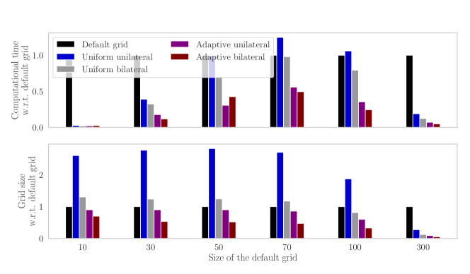
Figure 6: $\ell_{1}$ least-squares regression on the financial dataset E2006-log1p (available in libsvm) with $n=16087$ observations and $p=1668737$ features. We have used the same (vanilla) coordinate descent optimization solver with warm start between parameters for all grids. Note that a smaller grid do not imply faster computation, as the interplay with the warm-start can be intricate in our sequential approach.

References

• Arlot & Celisse (2010) Arlot, S. and Celisse, A. A survey of cross-validation procedures for model selection. Statistics surveys, 4:40–79, 2010.
• Azé & Penot (1995) Azé, D. and Penot, J.-P. Uniformly convex and uniformly smooth convex functions. In Annales de la faculté des sciences de Toulouse, pp. 705–730. Université Paul Sabatier, 1995.
• Bach et al. (2012) Bach, F., Jenatton, R., Mairal, J., and Obozinski, G. Convex optimization with sparsity-inducing norms. Foundations and Trends in Machine Learning, 4(1):1–106, 2012.
• Bauschke & Combettes (2011) Bauschke, H. H. and Combettes, P. L. Convex analysis and monotone operator theory in Hilbert spaces. Springer, New York, 2011. ISBN 978-1-4419-9466-0.
• Bottou & Bousquet (2008) Bottou, L. and Bousquet, O. The tradeoffs of large scale learning. In NIPS, pp.  161–168, 2008.
• Celeux et al. (2012) Celeux, G., Anbari, M. E., Marin, J.-M., and Robert, C. P. Regularization in regression: comparing bayesian and frequentist methods in a poorly informative situation. Bayesian Analysis, 7(2):477–502, 2012.
• Clarkson (2010) Clarkson, K. L. Coresets, sparse greedy approximation, and the frank-wolfe algorithm. ACM Transactions on Algorithms (TALG), 6(4):63:1–63:30, 2010.
• Efron et al. (2004) Efron, B., Hastie, T., Johnstone, I. M., and Tibshirani, R. Least angle regression. Ann. Statist., 32(2):407–499, 2004. With discussion, and a rejoinder by the authors.
• El Ghaoui et al. (2012) El Ghaoui, L., Viallon, V., and Rabbani, T. Safe feature elimination in sparse supervised learning. J. Pacific Optim., 8(4):667–698, 2012.
• Fercoq et al. (2015) Fercoq, O., Gramfort, A., and Salmon, J. Mind the duality gap: safer rules for the lasso. In ICML, pp.  333–342, 2015.
• Franceschi et al. (2018) Franceschi, L., Frasconi, P., Salzo, S., and Pontil, M. Bilevel programming for hyperparameter optimization and meta-learning. In ICML, pp.  1563–1572, 2018.
• Friedman et al. (2007) Friedman, J., Hastie, T., Höfling, H., and Tibshirani, R. Pathwise coordinate optimization. Ann. Appl. Stat., 1(2):302–332, 2007.
• Friedman et al. (2010) Friedman, J., Hastie, T., and Tibshirani, R. Regularization paths for generalized linear models via coordinate descent. J. Stat. Softw., 33(1):1, 2010.
• Gärtner et al. (2012) Gärtner, B., Jaggi, M., and Maria, C. An exponential lower bound on the complexity of regularization paths. Journal of Computational Geometry, 2012.
• Giesen et al. (2010) Giesen, J., Jaggi, M., and Laue, S. Approximating parameterized convex optimization problems. In European Symposium on Algorithms, pp.  524–535, 2010.
• Giesen et al. (2012) Giesen, J., Müller, J. K., Laue, S., and Swiercy, S. Approximating concavely parameterized optimization problems. In NIPS, pp.  2105–2113, 2012.
• Hastie et al. (2004) Hastie, T., Rosset, S., Tibshirani, R., and Zhu, J. The entire regularization path for the support vector machine. J. Mach. Learn. Res., 5:1391–1415, 2004.
• Hoerl & Kennard (1970) Hoerl, A. E. and Kennard, R. W. Ridge regression: Biased estimation for nonorthogonal problems. Technometrics, 12(1):55–67, 1970.
• Juditski & Nesterov (2014) Juditski, A. and Nesterov, Y. Primal-dual subgradient methods for minimizing uniformly convex functions. arXiv preprint arXiv:1401.1792, 2014.
• Kalnay et al. (1996) Kalnay, E., Kanamitsu, M., Kistler, R., Collins, W., Deaven, D., Gandin, L., Iredell, M., Saha, S., White, G., Woollen, J., et al. The NCEP/NCAR 40-year reanalysis project. Bulletin of the American meteorological Society, 77(3):437–471, 1996.
• Li et al. (2017) Li, L., Jamieson, K., DeSalvo, G., Rostamizadeh, A., and Talwalkar, A. Hyperband: A novel bandit-based approach to hyperparameter optimization. The Journal of Machine Learning Research, 18(1):6765–6816, 2017.
• Li & Singer (2018) Li, Y. and Singer, Y. The well tempered lasso. ICML, 2018.
• Mairal & Yu (2012) Mairal, J. and Yu, B. Complexity analysis of the lasso regularization path. In ICML, pp.  353–360, 2012.
• McCullagh & Nelder (1989) McCullagh, P. and Nelder, J. A. Generalized Linear Models. Chapman & Hall, 1989.
• Ndiaye (2018) Ndiaye, E. Safe optimization algorithms for variable selection and hyperparameter tuning. PhD thesis, Université Paris-Saclay, 2018.
• Ndiaye et al. (2017) Ndiaye, E., Fercoq, O., Gramfort, A., and Salmon, J. Gap safe screening rules for sparsity enforcing penalties. J. Mach. Learn. Res., 18(128):1–33, 2017.
• Nesterov (2004) Nesterov, Y. Introductory lectures on convex optimization, volume 87 of Applied Optimization. Kluwer Academic Publishers, Boston, MA, 2004.
• Osborne et al. (2000) Osborne, M. R., Presnell, B., and Turlach, B. A. A new approach to variable selection in least squares problems. IMA J. Numer. Anal., 20(3):389–403, 2000.
• Park & Hastie (2007) Park, M. Y. and Hastie, T. L1-regularization path algorithm for generalized linear models. J. Roy. Statist. Soc. Ser. B, 69(4):659–677, 2007.
• Pedregosa (2016) Pedregosa, F. Hyperparameter optimization with approximate gradient. In ICML, pp.  737–746, 2016.
• Pedregosa et al. (2011) Pedregosa, F., Varoquaux, G., Gramfort, A., Michel, V., Thirion, B., Grisel, O., Blondel, M., Prettenhofer, P., Weiss, R., Dubourg, V., Vanderplas, J., Passos, A., Cournapeau, D., Brucher, M., Perrot, M., and Duchesnay, E. Scikit-learn: Machine learning in Python. J. Mach. Learn. Res., 12:2825–2830, 2011.
• Rockafellar (1997) Rockafellar, R. T. Convex analysis. Princeton Landmarks in Mathematics. Princeton University Press, Princeton, NJ, 1997. Reprint of the 1970 original, Princeton Paperbacks.
• Rosset & Zhu (2007) Rosset, S. and Zhu, J. Piecewise linear regularized solution paths. Ann. Statist., 35(3):1012–1030, 2007.
• Shibagaki et al. (2015) Shibagaki, A., Suzuki, Y., Karasuyama, M., and Takeuchi, I. Regularization path of cross-validation error lower bounds. In NIPS, pp.  1666–1674, 2015.
• Shibagaki et al. (2016) Shibagaki, A., Karasuyama, M., Hatano, K., and Takeuchi, I. Simultaneous safe screening of features and samples in doubly sparse modeling. In ICML, pp.  1577–1586, 2016.
• Sun & Tran-Dinh (2017) Sun, T. and Tran-Dinh, Q. Generalized self-concordant functions: A recipe for newton-type methods. Mathematical Programming, 2017.
• Tibshirani (1996) Tibshirani, R. Regression shrinkage and selection via the lasso. J. Roy. Statist. Soc. Ser. B, 58(1):267–288, 1996.
• Zou & Hastie (2005) Zou, H. and Hastie, T. Regularization and variable selection via the elastic net. J. Roy. Statist. Soc. Ser. B, 67(2):301–320, 2005.