Concentration-dependent atomic mobilities in FCC CoCrFeMnNi high-entropy alloys

Abstract

The diffusion kinetics in a CoCrFeMnNi high entropy alloy is investigated by a combined radiotracer–interdiffusion experiment applied to a pseudo-binary Co₁₅Cr₂₀Fe₂₀Mn₂₀Ni₂₅ / Co₂₅Cr₂₀Fe₂₀Mn₂₀Ni₁₅ couple. As a result, the composition-dependent tracer diffusion coefficients of Co, Cr, Fe and Mn are determined. The elements are characterized by significantly different diffusion rates, with Mn being the fastest element and Co being the slowest one. The elements having originally equiatomic concentration through the diffusion couple are found to reveal up-hill diffusion, especially Cr and Mn. The atomic mobility of Co seems to follow an S-shaped concentration dependence along the diffusion path. The experimentally measured kinetic data are checked against the existing CALPHAD-type databases.
In order to ensure a consistent treatment of tracer and chemical diffusion a generalized symmetrized continuum approach for multi-component interdiffusion is proposed. Both, tracer and chemical diffusion concentration profiles are simulated and compared to the measurements. By using the measured tracer diffusion coefficients the chemical profiles can be described, almost perfectly, including up-hill diffusion.

I Introduction

In most of the engineering applications alloys are used which consist of one or two element(s) as the principal element(s) and they are supplemented with (typically minor) alloying elements to improve their physical and mechanical properties. However, multi-principal-element alloys were not preferred, since according to the Gibbs phase rule they lead potentially to formation of intermetallic compounds with usually brittle complex structures. A new class of multicomponent alloys, called high entropy alloys (HEAs), containing five or more principal elements in equiatomic or nearly equiatomic proportions promise to provide attractive mechanical properties including attractive strength-ductility combinations both at high- and low temperatures Murty2014 . Due to their high configurational mixing entropy ($\Delta S_{\text{mix}}$) HEAs were suggested to form fcc and/or bcc simple solid solution phases instead of complex intermetallic phases Yeh2004 .
As a counterpart to the configurational entropy, recent studies mention the importance of the formation enthalpy in determining the phase stability in HEAs. After Zhang et al. the high mixing entropy state does not always have the lowest Gibbs free energy Zhang2014 . Moreover, complex phases may precipitate in HEAs after long annealing treatments, typically at not too high temperatures. As well important as the configurational entropy are vibrational, electronic and magnetic contributions to the entropy, shown by ab-initio calculations for the CoCrFeMnNi alloy Ma2015 . Even short annealing of the severely plastically deformed CoCrFeMnNi alloy at a temperature of $450^{\circ}$C results in a phase decomposition, suggesting that a high mixing entropy does not guarantee the phase stability Schuh2015 ; Otto2016 . Furthermore, the single phase observed in HEAs might be a high temperature phase with a kinetically constrained transformation Schuh2015 .
Focusing on high temperature mechanical properties Guo2016 ; Chen2016 , creep strength Lee2016 ; Zhang2016 ; Ma2016 ; Cao2016 , oxidation resistance Kai2016 ; Laplanche2016 ; Holcomb2015 and coating applications Shaginyan2016 , numerous HEAs have been investigated following an originally introduced paradigm of four ’core’ effects, i.e. a high entropy, severe lattice distortion, ’cocktail’ effect and ’sluggish’ diffusion Yeh2004 . These basic principles are questioned now Pickering2016 ; cors , nevertheless the understanding of the diffusion kinetics in HEAs, which is assumed to be responsible for the unique features like excellent thermal stability, decelerated grain growth, formation of nano-precipitates Murty2014 and an excellent resistance to grain coarsening in a nanocrystalline CoCrFeNi alloy Praveen2016 , is of fundamental significance.
The present knowledge about diffusion in HEAs is limited to few interdiffusion investigations in couples or multiples Tsai2013 ; Kulkarni2015 ; Dabrowa2016 and direct radiotracer diffusion measurements in polycrystalline and single crystalline CoCrFeNi and CoCrFeMnNi Vaidya2016 ; Vaidya2017 ; Vaidya2018 ; Gaertner2018 . Interdiffusion coefficients in a CoCrFeMn_0.5Ni alloy were determined using a quasi-binary approach Tsai2013 , originally known as pseudo-binary approach Paul2013 , proposing the evaluated diffusivities to be approximately equal to the intrinsic and tracer diffusivities of the equiatomic CoCrFeMnNi alloy with a thermodynamic factor of about unity Tsai2013 . In fact, this assumption was found to be correct in the framework of the random alloy model Murch2017 . However, the basic principles of the analysis by Tsai et al. Tsai2013 were seriously questioned recently Review . The direct radiotracer measurements, being focused on measuring the bulk and short-circuit diffusion rates of the constituting elements in absence of any chemical interaction due to low diffusant concentrations, are preferable but typically limited to single compositions of the given alloy system. Moreover, recently it was shown that the thermodynamic factor (more specifically the product of the thermodynamic factor and the vacancy wind effect), being indeed about unity in CoCrFeNi, deviates strongly from unity in CoCrFeMnNi Vaidya2018S .
In metallic materials the diffusion model implemented in the DICTRA (Diffusion Controlled Phase Transformation) software is the most common continuum model based on a sublattice description Agren1982 ; Andersson1992 ; Borgenstam2000 . In a three dimensional setting nowadays the multicomponent multiphase-field method with an integrated sublattice description is applied to phase transformations and microstructural evolution Zhang2015 . In both implementations diffusion is combined with CALPHAD (Calculation of Phase Diagrams) type thermodynamic and kinetic databases to account for temperature and composition dependent Gibbs energies and atomic mobilities Lukas2010 ; Campbell2001 . The DICTRA diffusion model is based on a reference element, which is predefined in most alloys by its principal element. In case of equiatomic alloys, like HEAs, the selection of a reference element is arbitrary. Several databases were developed for different main elements, e.g TCNI Ni-based Superalloys Database or Thermo-Calc Software TCFE Steels/Fe-alloys Database. They can be extrapolated into the equiatomic region but this can lead to inaccuracies. Currently thermodynamic databases especially designed for HEAs were published: Thermo-Calc Software TCHEA3 Database TCHEA3 and another one developed by Hallstedt’s group Haase2017 . Furthermore a mobility database (Thermo-Calc Software MOBHEA1 Database TCHEA_dat ) was published, which is based on the MOBNI4 mobility database TCNI_dat .

The present work is focused on combined radiotracer and interdiffusion experiments in HEAs determining the concentration dependent tracer diffusion coefficients without estimation of the interdiffusion coefficients, that would be conceptually hindered due to appearance of up-hill diffusion effects. Simulations of both, the radiotracer and interdiffusion concentration profiles were performed using a new generalized multi-component diffusion model. This so-called pair-wise diffusion model (PD-model) is shown to be especially appropriate for the compositions about equiatomic ones that makes the model particularly suitable for HEAs. In the binary case and in the dilute limit it reduces to the DICTRA model. The simulations are used to compare the existing databases, with a special focus on multi-component diffusion kinetics and cross correlation effects, with the newly determined composition dependent tracer diffusion coefficients. The simulations show the importance of accurately measured kinetic data combined with an appropriate diffusion model and a database.

II Experimental procedure

II.1 Sample preparation

Polycrystalline Co₁₅CrFeMnNi₂₅ and Co₂₅CrFeMnNi₁₅ samples were produced by arc melting of a mixture of pure elements and homogenized subsequently at $1473$ K for $48$ hours under purified Ar atmosphere. Here and below the element concentrations are given in at.% and, if not explicitly specified by a proper sub-index, the element concentration is equal to 20 at.%, that corresponds to an equiatomic composition of the quinary alloy.
Cylindrical samples with a diameter of $8$ mm and a thickness of $1.7$ mm (Co₁₅CrFeMnNi₂₅) and $0.7$ mm (Co₂₅CrFeMnNi₁₅) were cut by spark-erosion and etched carefully with aqua regia to remove any contamination. The opposite faces of each specimen were polished by a standard metallographic procedure to a mirror-like quality. A diffusion couple was assembled by fixing the two samples and pressing them together by screws in a steel tube. Tungsten discs were used as separators between the fixture and the samples. Two identical couples – one for the radiotracer and one for the interdiffusion experiments – were prepared in order to prevent any radioactive contamination of the electron probe microanalyzer (EPMA). The preparation of couples was performed in a glove-box under a pure nitrogen atmosphere with $\approx 1.5$ mbar over-pressure.
The assembled fixture was sealed into silica tubes under a purified ($5$N) Ar atmosphere and subjected to the diffusion annealing at a temperature of $1373$ K for $48$ hours. The temperature was measured and controlled by a Ni–NiCr thermocouple to an accuracy of $\pm 1$ K.

II.2 Interdiffusion experiment

After the diffusion annealing, one couple was embedded in epoxy and cut perpendicular to the surface in two halves using a diamond wire saw. The halved disks were then embedded in a conductive epoxy. Measurements using a CAMECA SX100 EPMA were carried out at an accelerating voltage of $15$ kV and a beam current of $40$ nA using pure standards for all elements. In order to measure the concentration profiles of the constituting elements multiple dedicated line-scans perpendicular to the interface between both sample parts were performed. The line-scans were set to a total length of $400$ $\mu$m – approximately $200$ $\mu$m in each sample half – with a step size of $1$ $\mu$m.

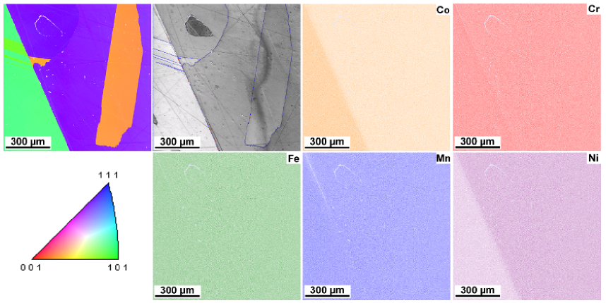
Figure 1: Orientation imaging microscopy at the interface of the Co₂₅CrFeMnNi₁₅-Co₁₅CrFeMnNi₂₅ HEA couple and the corresponding elemental maps obtained by EDX analysis. The grain orientations are colored according to the inverse pole figure (bottom left panel).

II.3 Radiotracer experiment

The radiotracers ⁵⁷Co, ⁵¹Cr, ⁵⁹Fe and ⁵⁴Mn were available as HCl solutions. The original solutions were highly diluted with double-distilled water achieving the required specific activity of the tracer material. A mixture of the tracers (⁵⁷Co$+^{51}$Cr$+^{59}$Fe$+^{54}$Mn) with the radioactivity of about $5$ kBq for each tracer was applied on each polished sample surface and dried. Subsequently the diffusion couple was assembled as described above and subjected to the given diffusion annealing treatment. Since all elements whose radioactive isotopes are used are already present in the compound, their simultaneous application does not induce any additional cross-correlation effects. Therefore, reliable data on tracer diffusion coefficients in the alloys were obtained. Since the available ⁶³Ni radioisotope emmits only $\beta$-quanta, its decays cannot be recorded by the $\gamma$-spectrometry. A separate (i.e. third) experiment would be required that is a subject for future work.
After the diffusion annealing, the diffusion-bonded couple was reduced in diameter by about $1.5$ mm in order to remove the effects of lateral and surface diffusion. The penetration profiles were determined by precise parallel mechanical sectioning using a grinding machine and grinding paper with SiC grains of about $30$ $\mu$m. Before and after sectioning the section masses were determined by weighing the samples on a microbalance to an accuracy of $0.1\,\mu$g.
The sectioning began from the Co₁₅CrFeMnNi₂₅ alloy (which was prepared as a thicker disc) by gluing the Co₂₅CrFeMnNi₁₅ side to a holder. As soon as the background for all isotopes was reached, the sectioning was stopped. Then the couple was dismounted from the holder, reverted and glued again to the holder by the Co₁₅CrFeMnNi₂₅ side. Afterwards, the sectioning was continued from the Co₂₅CrFeMnNi₁₅ side till the Matano plane was reached (that corresponded to an increase of the radioactivity) and then till background was approached again. This approach allowed to measure in a single experiment three concentration profiles: two profiles for tracer diffusion in the unaffected end-members of the couple and one profile corresponding to tracer diffusion in both directions from the Matano plane which proceeded parallel to the chemical interdiffusion.
A density variation induced in the alloy by chemical diffusion was neglected that introduces an uncertainty in the depth coordinate $y$ below $1$ %. Since the initial thicknesses of the samples were carefully measured, a continuous coordinate $y$ through the whole couple was in fact determined.
The relative radioactivity of each section was measured by an available pure Ge $\gamma$-detector equipped with a $16$ K multi-channel analyzer. All used radioisotopes, ⁵⁷Co, ⁵¹Cr, ⁵⁹Fe and ⁵⁴Mn, decay emitting the $\gamma$-quanta whose energies Lemmer1955 ; Ofer1957 ; Heath1960 ; Lederer1978 can easily be discriminated by the available setup with the energy resolution of about $0.7$ eV. The relative radioactivities for each isotope were carefully determined by the background subtraction, including the Compton scatter.
The tracer concentration in a section is proportional to the section activity divided by the section mass. As a result, the tracer concentration profiles, $c^{*}_{E}(y)$, were determined where $E$ is the corresponding element, i.e. ⁵⁷Co, ⁵¹Cr, ⁵⁹Fe or ⁵⁴Mn.

III Experimental results

III.1 Microstructure analysis

The microstructure and the chemical composition of the couple near the interface after diffusion annealing was examined by orientation imaging microscopy using Electron Back-Scatter Diffraction (EBSD) and Energy Dispersive X-Ray Spectroscopy (EDX). Figure 1 presents the region where the original interface between both high-entropy alloys was located and shows the grain orientation mapping using the inverse pole figure (bottom left) and the chemical maps. The grains were found to be larger than $500$ $\mu$m on average and the chemical maps verify the homogeneity of the equiatomic constituents in both alloys far from the Matano plane and chemical gradients of Co and Ni at the interface. Furthermore, the chemical maps reveal several local thin gaps between the two alloys (e.g. top left corner of the given chemical maps). At such gaps the Mn concentration tends to be decreased. However, these spurious gaps are relatively small and localized and both alloys are almost in perfect contact. At the positions with a perfect contact (and simultaneously far from any grain boundary) the EPMA analysis was performed. Correspondingly, composition profiles corresponding to true volume interdiffusion were determined.

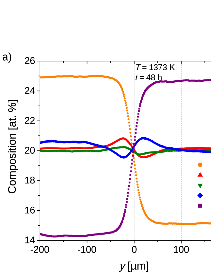
Figure 2: a) EPMA-analysis of the constituents at the interface and b) penetration profiles measured for tracer ⁵⁷Co, ⁵¹Cr, ⁵⁹Fe and ⁵⁴Mn diffusion (open symbols) from the outer surfaces and the internal source located at the original interface between the two alloys (the Gaussian fits are represented by the straight lines). In b) the tracer profiles are shifted by multiplication with a constant factor for a better readability.

III.2 Diffusion experiments

III.2.1 EPMA interdiffusion measurements

Figure 2a shows the concentration profiles of all constituting elements measured by electron probe microanalysis. Each profile was smoothed using the Savitzky-Golay filter method performing a local second order polynomial regression over $50$ data points.
The origin of the depth coordinate $y$ was set at the position of the Matano plane Mehrer2007 of Co using

$$(c_{\text{L}}-c_{\text{R}})y_{\text{M}}+\int_{c_{\text{L}}}^{c_{\text{M}}}ydc+\int_{c_{\text{M}}}^{c_{\text{R}}}ydc=0,$$ (1)

with $c_{\text{L}}$ being the concentration on the left-hand side, $c_{\text{R}}$ the concentration on the right-hand side, $c_{\text{M}}$ the concentration at the Matano plane and $y_{\text{M}}$ the position of the Matano plane. The position of the Matano plane was almost the same within the experimental uncertainties when determined using the Ni concentration profile, as it should be for a pseudo-binary couple Paul2013 . However, a careful inspection of the concentration profiles in Fig. 2a reveals that we are dealing with a non-ideal pseudo-binary couple (in terms of Ref. Review ) since the Ni and Mn concentrations in the nominally Co₂₅CrFeMnNi₁₅ alloy deviate by less than $0.4$ at.% from their nominal values.

A remarkable feature is the appearance of up-hill diffusion in the concentration profiles of the nominally equiatomic constituents Cr, Fe and Mn. Especially, the Cr- and Mn-concentration profiles show distinct and oppositely directed up-hill diffusion, Fig. 2a.
The radiotracer experiment with combined interdiffusion was performed separately under the same conditions like the sole interdiffusion experiment, at $1373$ K for $48$ hours. The tracer solutions were applied on all four polished sample surfaces.

III.2.2 Tracer diffusion measurements

Figure 2b shows the measured penetration profiles for tracer diffusion of ⁵⁷Co, ⁵¹Cr, ⁵⁹Fe and ⁵⁴Mn. The origin of the $y$ coordinate is set at the interface of the diffusion couple which roughly corresponds to the Matano plane in Fig. 2a. A slight disagreement between the $y$ scales in Figs. 2a and b stems from the accuracy of sample’s thickness measurements, (non-propagating!) error of thickness determination of individual sections and the accuracy of the sample orientation for grinding perpendicular to the diffusion direction.
A comparison of Figs. 2a and b substantiates that outer tracer concentration profiles are located in regions without any influence of the chemical driving force and correspond to diffusion in not-affected end-members of the couple. Therefore, the corresponding tracer concentrations have to follow a thin film solution of the diffusion problem Mehrer2007 ,

$$c^{*}_{E}(y,t)=\frac{M_{E}}{\sqrt{\pi D^{*}_{E}t}}\exp{\left(-\frac{(y-y_{0})^{2}}{4D^{*}_{E}t}\right)}$$ (2)

where $M_{E}$ denotes the initial amount of the tracer $E$, $c^{*}_{E}$ the concentration of the tracer $E$ in the layer, which is proportional to the relative specific activity of the tracer, $y_{0}$ the origin of the diffusion source, i.e. the left or right end of the couple, and $D^{*}_{E}$ the corresponding volume diffusion coefficient. Excepting few very first data points, all concentration profiles follow the Gaussian solutions over two to three orders of magnitude in decrease of the tracer concentration, as indicated by the solid lines in Fig. 2b.
At larger depths, all penetration profiles – both the outer concentration profiles for end-members as well as the interface-related concentration profiles – reveal the existence of second, fast-diffusion branches. These branches correspond to grain boundary diffusion in the polycrystalline alloys as it was observed in our previous measurements of volume diffusion in CoCrFeNi and CoCrFeMnNi alloys Vaidya2016 ; Vaidya2018 . In the present report we are focused on the volume diffusion branches.
The solid lines in Fig. 2b represent the expected Gaussian solutions of the first diffusion branches which represent the true volume diffusion. From the fits, the tracer volume diffusion coefficients, $D^{*}_{E}$, of all elements can be determined. The corresponding parameters of the tracer diffusion experiments and the determined diffusion coefficients in the unaffected end-members are summarized in Table 1 for the Co₂₅CrFeMnNi₁₅ and Co₁₅CrFeMnNi₂₅ high-entropy alloys. For comparison, the tracer diffusion coefficients measured for equiatomic CoCrFeMnNi alloys Gaertner2018 are given, too.

Table 1: Tracer volume diffusion coefficients $D^{*}$ (in $10^{-15}$ m²s^-1) measured for the Co₂₅CrFeMnNi₁₅ and Co₁₅CrFeMnNi₂₅ high-entropy alloys at $1373$ K using unaffected end-members. The uncertainty of the $D^{*}$ values is typically below $20\,\%$. For comparison the averaged tracer diffusion coefficients determined for single crystalline equiatomic CoCrFeMnNi HEA Gaertner2018 are shown, too.

Alloy	Co	Cr	Fe	Mn	Ref.
Co25CrFeMnNi15	$1.2\pm 0.1$	$3.9\pm 0.1$	$2.4\pm 0.1$	$8.2\pm 0.2$	present work
Co15CrFeMnNi25	$2.1\pm 0.1$	$5.6\pm 0.1$	$4.2\pm 0.1$	$13.3\pm 0.6$	present work
CoCrFeMnNi	$1.9\pm 0.2$	$5.0\pm 0.6$	$3.4\pm 0.5$	$9.0\pm 1.0$	Gaertner2018

In both alloys, Mn is found to be the fastest element and Co the slowest one (note that Ni tracer diffusion was not measured in the present work). Table 1 suggests further that the diffusion rates of all investigated elements are increased by up to $75\,\%$ after alloying the opposite amount of Co and Ni, while keeping an equiatomic ratio of the other three elements. A direct comparison of the tracer and chemical profiles in the vicinity of the Matano plane reveals immediately significantly different scales on which volume diffusion could reliably be followed. Indeed, if ⁵⁴Mn tracer diffusion is measurable in the region of $\pm 400\,\mu$m and it is $\pm 100\,\mu$m for ⁵⁷Co, the chemical changes are confined within $\pm 80\,\mu$m from the initial interface, see Fig. 2.

III.2.3 Combined tracer-interdiffusion measurements

In order to analyze the tracer concentration profiles of all constituting elements developed at the original interface of the pseudo-binary couple, the Gaussian solution, Eq. (2), is invalid due to a strong chemical driving force. The concentration-dependent tracer diffusion coefficients can be determined using the framework of a thin layer isotope sandwich configuration Belova2015 ,

$$D^{*}_{E}(c)=-\frac{\frac{(y+a)}{2t}-\frac{G_{E}(y)}{c_{E}(y)}}{\frac{\partial\ln c^{*}_{E}(y)}{\partial y}-\frac{\partial\ln c_{E}(y)}{\partial y}}$$ (3)

where $c_{E}(y)$ is the concentration of the element $E$, $c^{*}_{E}(y)$ the tracer concentration of the same element, $G_{E}(y)$ is the value proportional to the flux of the element $E$. The value of the parameter $a$ corresponds to a misfit of the $y$ scales for the chemical, $c_{E}(y)$, and the tracer, $c^{*}_{E}(y)$, profiles and $a$ can be determined from the condition that the tracer diffusion coefficient $D^{*}_{E}(c)$ is positive at all $y$. Making use of the Sauer-Freise method Sauer1962 the factor $G_{E}(y)$ can be determined Belova2015 ,

$$G_{E}(y) = \frac{c_{\text{R}}-c_{\text{L}}}{2t}\times\left[(1-Y_{E})\int_{-\infty}^{y}Y_{E}dy+\right.$$ (4)

$$\left.Y_{E}\int_{y}^{\infty}(1-Y_{E})dy\right]$$

where $Y_{E}(y)=(c_{E}(y)-c_{\text{L}})/(c_{\text{R}}-c_{\text{L}})$ is the reduced concentration of the given chemical element $E$. A variation of the molar volume with composition is neglected, which is a reasonable approximation in the present case.
In Fig. 3, the determined concentration-dependent tracer diffusion coefficients are shown as straight lines. The profiles show peak-like artefacts resulting from the amount of data points and the fitting of the parameter $a$ in Eq. 4. Since the interdiffusion coefficients determined by the Sauer-Freise method are typically prone to large uncertainties for the compositions close to the end-members, the corresponding values are indicated as dotted lines in Fig. 3.

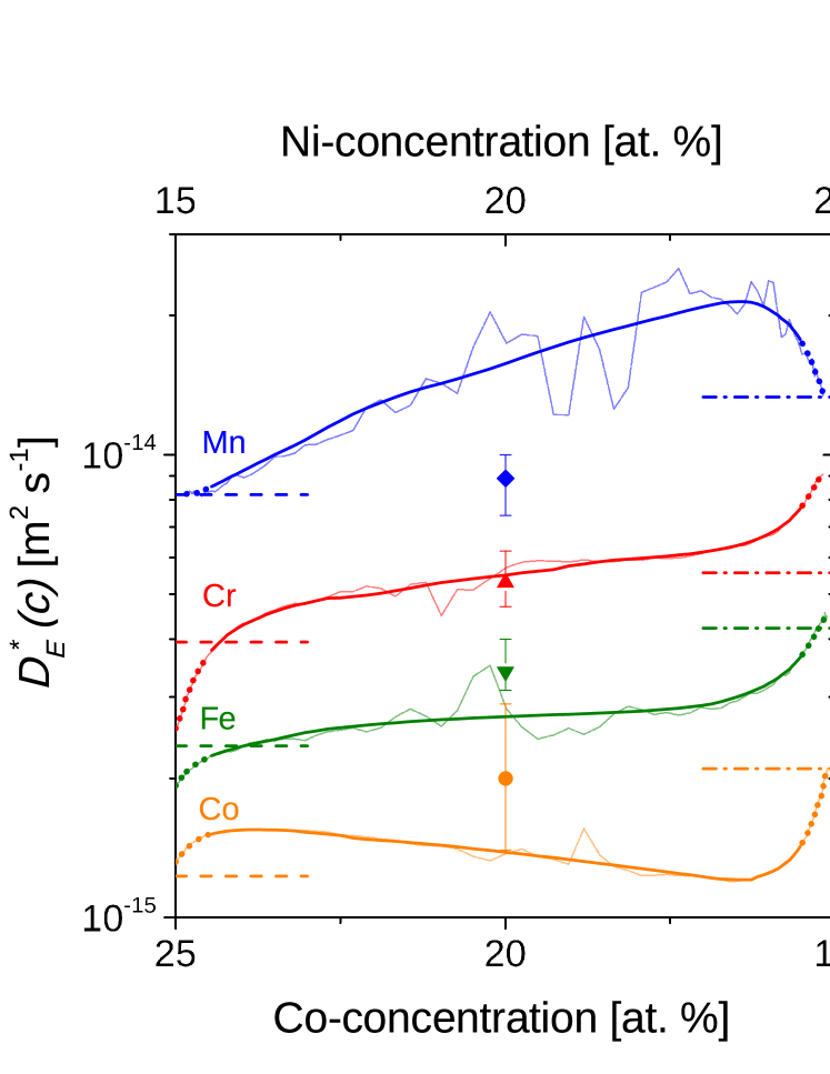
Figure 3: Tracer diffusion coefficients of Co, Cr, Fe and Mn as a function of the Co-concentration (represented by solid lines) compared with the tracer diffusion coefficients measured in the sides with constant constituent concentration (represented by dashed lines for the Co-rich side and dashed-dot lines for the Ni-rich side) and with the tracer diffusion coefficients measured in single crystalline CoCrFeMnNi HEA Gaertner2018 (represented by filled symbols). The dotted lines show the determined tracer diffusion coefficients for the near end-member compositions.

The concentration dependent tracer diffusion coefficient of Co shows a S-shaped trend and the independently measured diffusion coefficients for the end-member concentrations, represented by the dashed and dashed-dotted lines for the Co-rich and Ni-rich sides, respectively, are in a good agreement with the determined trends within the typical accuracy of about $20\,\%$ for the tracer experiments.
The present analysis predicts a clear decrease of the Co tracer coefficient with decreasing Co concentration from $23$ to $17\,\text{at.}\leavevmode\nobreak\ \%$. Contrary to that, the other elements show an increase of the diffusion rate in this concentration range, especially if the near-end member concentrations are not included in the analysis. This Co behavior is the subject of an ongoing work in a pseudo-binary couple with Co₂₃CrFeMnNi₁₇ and Co₁₇CrFeMnNi₂₃ HEAs.
The independently determined tracer diffusion coefficients, i.e. those for the end-members, Eq. 2, and along the diffusion path, Eqs. 3 & 4, for Mn are in a good agreement, while the deviations are larger for Cr and Fe.
The tracer diffusion coefficients measured in equiatomic single crystalline CoCrFeMnNi HEA Gaertner2018 are shown as filled symbols in Fig. 3. In case of Co and Fe the volume diffusion coefficients are higher than the corresponding coefficients $D^{*}_{E}(c)$, however, the values overlap accounting for the measurement uncertainties. The coefficient $D^{*}_{\text{Cr}}(c)$ is in very good agreement with the single crystal data for Cr, while the Mn volume diffusion coefficient in the equiatomic state is somewhat overestimated. This relatively large deviation of about $50\,\%$ may probably result from the strong up-hill diffusion contribution.

IV Diffusion simulations

IV.1 Model description

IV.1.1 Pair-wise diffusion model

In the present work, a generalized diffusion model, which is independent of a reference element, is proposed. The fluxes given in the lattice-fixed frame are transformed into the laboratory-fixed frame following the approach of Boettinger et al. Boettinger2016 who derived the flux equations for the binary case. Extending it to the multi-component case and using the assumption that all partial molar volumes are equal and independent of composition, as it was done for the analysis of the experimental data above, the fluxes can be written in the following pair-wise form (for a short derivation see the Appendix A, a detailed derivation and analysis of the resulting diffusion equation will be published elsewhere):

$$\tilde{J}_{i} = -\frac{1}{2}\sum_{j}^{n}x_{i}x_{j}M_{ij}(\nabla\mu_{i}-\nabla\mu_{j})=$$ (5)

$$-\frac{1}{2}\sum_{j}^{n}x_{i}x_{j}M_{ij}\nabla\tilde{\mu}_{ij}$$

with $x_{i}$ as the mole fraction of element $i$, $M_{ij}$ is the concentration-dependent pair-exchange mobility and $\mu_{i}$ the chemical potential of element $i$. The change of composition is then given as:

$$\frac{\partial x_{i}}{\partial t}=-\nabla\tilde{J}_{i}=\frac{1}{2}\nabla\sum_{\begin{subarray}{c}j=1\\ j\neq i\end{subarray}}^{n}x_{i}x_{j}M_{ij}\nabla\tilde{\mu}_{ij}.$$ (6)

The sum is taken over all pairs of elements. The key point of the present ansatz is that the thermodynamic driving force is given by the gradient of the difference of the chemical potentials of each pair:

$$\tilde{\mu}_{ij}=\mu_{i}-\mu_{j}=\frac{\partial G}{\partial x_{i}}-\frac{\partial G}{\partial x_{j}}.$$ (7)

$M_{ij}$ is the pair-exchange mobility of element $i$ and $j$. It represents the exchange rate of solutes through a unit area within the reference volumina at the continuum scale, and should not be confused with an atomistic pair-exchange mechanism. It may be due to an atomistically defined vacancy mechanism with ’many’ individual jumps, or other mechanisms. The key idea is to decompose a general multi-solutal diffusion process in pairs of exchange processes with a common reference in the diffusion potential.

Pair-exchange mobility $M_{ij}$
The pair-exchange mobility can be derived by transforming the intrinsic fluxes in the lattice-fixed frame of reference $J_{i}=-M_{i}\frac{x_{i}}{V_{m}}\nabla\mu_{A}$ into the laboratory frame $\tilde{J_{i}}$ including the velocity with which the frames move with respect to each other. Rewriting the resulting flux as pair-wise contributions, given in Eq. 6, the pair-exchange mobility is defined as:

$$M_{ij}=x_{i}M_{j}+x_{j}M_{i}+\sum_{\begin{subarray}{c}k=1\\ k\neq i\\ k\neq j\end{subarray}}^{n}x_{k}(M_{i}+M_{j}-M_{k})$$ (8)

with $M_{k}$ as the concentration-dependent atomic mobility of element $k$. Note that for large differences in the mobilities of different elements, in particular $M_{k}$ $\gg$ $M_{i}$, $M_{j}$, the pair mobility $M_{ij}$ can become negative. In general, this is not a problem, since one has to ensure that the diffusion matrix is positively defined for consistency with the second law of thermodynamics. See also recent discussion in Chen2018 .
It can be directly seen that the introduced pair-exchange mobilities are symmetric: $M_{ij}$ = $M_{ji}$. In the binary case the pair-exchange mobility reduces to $M_{ij}=x_{i}M_{j}+x_{j}M_{i}$. In higher order systems, additional to the binary pair-exchange mobility, a term over all other elements except $i$ and $j$ (second part of Eq. 8) influences the pair-exchange mobility between $i$ and $j$. The diagonal terms ($M_{ii}$) are not defined. It is shown in Appendix B, that the generalized pair-wise diffusion model reduces to the DICTRA model Andersson1992 in the dilute solution limit.

Atomic mobility $M_{i}$
The pair-exchange mobility $M_{ij}$ can be constructed from the composition dependent atomic mobilities $M_{i}$, see Eq. 8. In 1992 Andersson and Ågren Andersson1992 proposed to store the temperature and composition dependent atomic mobilities in CALPHAD-type kinetic databases and model the temperature dependence as Andersson1992 ; Campbell2001 :

$$M_{i}=\frac{1}{RT}M_{i}^{0}\exp{\bigg{(}-\frac{Q_{i}}{RT}\bigg{)}}\left[{}^{\text{mag}}\Gamma_{i}\right].$$ (9)

R is the gas constant, T the temperature, $M_{i}^{0}$ the frequency factor, $Q_{i}$ the activation energy for diffusion and ${}^{\text{mag}}\Gamma_{i}$ the magnetic contribution (set to unity in the present case). It is customary in most kinetic databases to include the composition dependence in $Q_{i}$ using Redlich-Kister polynomials, while $M_{i}^{0}$ is equal 1 Campbell2001 ; Redlich1948 :

$$Q_{i}=\sum_{j}x_{j}Q_{i}^{j}+\sum_{p}\sum_{j>p}x_{p}x_{j}\sum_{k}A_{i}^{pj}(x_{p}-x_{j})^{k}$$ (10)

with $Q_{i}^{j}$ and $A_{i}^{pj}$ as fit parameters. Nearly every temperature and composition-range in most phases is covered either by assessments or by extrapolating the existing data to the given system using the described scheme for composition and temperature dependence.
In this paper not only kinetic databases are used to describe the atomic mobilities but also direct use is made of the experimentally measured tracer diffusion coefficients $D_{i}^{*}$, applying the Einstein relation:

$$M_{i}(c)=\frac{D_{i}^{*}(c)}{RT}.$$ (11)

Taking advantage of the particular set-up of the modified tracer-interdiffusion couple (MTIC) experiment, i.e. the diffusion measurements within the interdiffusion zone and in the unaffected end-members (see Fig. 2), two different data repositories, applicable for the diffusion simulations in the given composition-range, are established:
1. The tracer diffusion coefficients determined from the measurements in the unaffected end-members (see Table 1) are linearly interpolated and stored in the data repository called MTIC-Lin (the functions are given in Appendix C).
2. The concentration-dependent tracer diffusion coefficients determined along the interdiffusion path using the Belova-Murch approach Belova2015 (shown in Fig. 3) which cover the investigated composition range and make an interpolation redundant, are directly used. This data repository is referred to as MTIC-BM in the following.
These two approaches allow a direct use of the experimentally measured kinetic data in the diffusion simulations. It is possible to rewrite the data in Redlich-Kister polynomials as it is done for CALPHAD-type kinetic databases (in Appendix C the Redlich-Kister polynomials are given as an example for MTIC-Lin).

IV.1.2 Tracer diffusion simulations

Thermodynamic and kinetic model for tracer atoms
In the following simulations the mass effect of isotopes on diffusion is neglected. Therefore the radioactive tracer atoms are chemically indistinguishable from the stable isotopes (non-tracer) of the same species and their thermodynamic and kinetic properties are considered to be the same. The total composition of one species is then given by:

$$x_{i,\text{tot}}=x^{*}_{i}+x_{i}.$$ (12)

$x^{*}_{i}$ is the tracer concentration of species $i$ and $x_{i}$ is the amount of non-tracer atoms of species $i$. Thermodynamic and kinetic properties are always evaluated with respect to $x_{i,\text{tot}}$. Pair-wise diffusion is applied to $x_{i,\text{tot}}$ and does not distinguish between $x^{*}_{i}$ and $x_{i}$. Therefore the pair-wise model does not take into account self-diffusion of tracer atoms (the corresponding difference of the chemical potential gradients is $\mu_{i^{*}}-\mu_{i}=0$).

Self-diffusion model
To take into account self-diffusion of tracer atoms, a second diffusion model is used. There is no explicit exchange between different isotopes of the same element within the pair-exchange model as mentioned above. With the aim to reproduce experimentally measured tracer profiles one can safely assume that the amount of tracer atoms used in the experiments is too small to influence the overall concentration in a measurable amount (for EPMA analysis), see Eq. 13 that was verified by direct estimates of the absolute concentrations of tracer atoms in a diffusion experiment Divinski2001 . The key point is that self-diffusion is measured and no impurities - which may effect the vacancy concentration especially in non-metallic systems - are introduced by application of tracer solutions. Therefore cross terms can be neglected and one can assume an ideal solution model. Self-diffusion can then be described with Fick’s second law:

$$\frac{\partial x_{i}^{*}}{\partial t}=\nabla\left[D_{i}\nabla x_{i}^{*}\right].$$ (13)

$x_{i}^{*}$ is the concentration of the tracer atoms of species $i$ and $D_{i}$ is the self-diffusion coefficient of element $i$ (composition dependence is evaluated with respect to the total composition). Applying the fluctuation-dissipation theorem Kubo1966 $D_{i}$ shall be identified with $D_{i}^{*}$ in Eq. 11.

Figure 4: Comparison between experimentally measured interdiffusion profiles and simulated ones using the three different thermodynamic/kinetic databases (compare Table 2) for all five elements (Co, Cr, Fe, Mn and Ni) after 48 h at 1373 K.

IV.2 Simulation results

In the following simulations the annealing time and duration were chosen for comparability as in the experiment (1373 K, 48 h). The pair-wise ansatz for chemical diffusion and tracer diffusion in varying chemical composition are solved explicitly using adaptive time stepping with a constant grid spacing ($1\,\mu m$). The box size of the 1D simulations were chosen to represent a semi-infinite sample where the concentrations at the ends are not affected by interdiffusion. Fixed concentrations were taken as boundary conditions. The initial amount of tracer ($x_{i}^{*}$) does not influence the profiles as long as it is smaller than the overall concentration of the given element ($x_{i}^{*}\leq x_{i,\text{tot}}$). To minimize numerical errors, the initial tracer distribution amount was chosen as $x_{i}^{*}=0.25\cdot\delta(y)$ for Co, Cr, Fe and Mn, with $\delta(y)$ as the Dirak-delta function and the distance $y$.
In the sublattice representation of CoCrFeMnNi all elements in the fcc lattice are on the substitutional sublattice and the interstitial sublattice is only occupied by vacancies (Co, Cr, Fe, Mn, Ni)₁(Va)₁. Three different sets of databases (thermodynamic + kinetic database) are investigated in the following simulations (summarized in Table 2). TCNI8/MOBNI4 TCNI_dat and TCFE9/MOBFE4 TCFE_dat were developed for alloys with Ni respectively Fe as principal element. Another thermodynamic database was developed by Hallstedt’s group (in the following abbreviated by HEA-DB) especially for HEAs Haase2017 . Due to the lack of an explicit HEA kinetic database it was also combined with the MOBNI4 TCNI_dat database. The HEA databases developed by Thermo-Calc TCHEA_dat were not considered in this work, due to the availability of the HEA-DB.

Table 2: Combinations of thermodynamic and kinetic databases used in the following simulations. For the combination HEA-DB/MOBNI4, Ni as reference element is given in brackets, because only the kinetic database is based on a reference element: Ni.

Thermodynamic Database	Kinetic Database	Reference Element
TCNI8 TCNI_dat	MOBNI4 TCNI_dat	Ni
TCFE9 TCFE_dat	MOBFE4 TCFE_dat	Fe
HEA-DB (Hallstedt’s group) Haase2017	MOBNI4 TCNI_dat	(Ni)

IV.2.1 Interdiffusion

The experimentally measured and simulated interdiffusion profiles using the three different database combinations given in Table 2 are shown in Fig. 4.

Co and Ni
The simulated profiles for Co and Ni are for all database combinations considerably shallower than the experimentally measured profiles. Using TCNI8/MOBNI4 and HEA-DB/MOBNI4 the predicted profiles nearly coincide for both elements. For Co the simulated profile using TCFE9/MOBFE4 is closer to the experimental result than the others. For Ni, all database combinations provide nearly similar descriptions strongly deviating from the experimental profile.

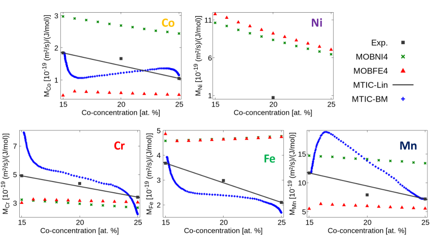
Figure 5: Composition dependent atomic mobilities for Co, Cr, Fe, Mn and Ni. Cr, Fe and Mn concentration is assumed to be constant ($20$ at.$\,\%$ each). The grey squares are the values determined from the experiments in constant composition (compare Table 1) and a linear interpolation between the end points is shown as solid line (MTIC-Lin). MTIC-BM (blue crosses) represents the result from the modified tracer-interdiffusion couple.

Cr, Fe and Mn
For the three elements Cr, Fe and Mn, uphill diffusion was observed in the experiment and is also observed in the simulations. For Cr and Fe the simulated results reveal uphill diffusion in the opposite direction than the experiment (Experiment: uphill diffusion along the concentration gradient of Ni; Simulations: uphill diffusion against the concentration gradient of Ni - see Fig. 4). The different databases are only distinct from each other in the magnitude of the uphill profile. For Mn the simulated profiles using TCFE9/MOBFE4 and HEA-DB/MOBNI4 show uphill diffusion in the same direction as the experiment while for TCNI8/MOBNI4 the profile is rather flat.

It should be noted that the database combinations TCNI8/MOBNI4 and TCFE9/MOBFE4 were not developed for the equiatomic composition range. But although the HEA-DB thermodynamic database was developed for the given composition range, simulations using this database cannot reproduce the experimentally measured profile, which might be due to the not fitting kinetic database.

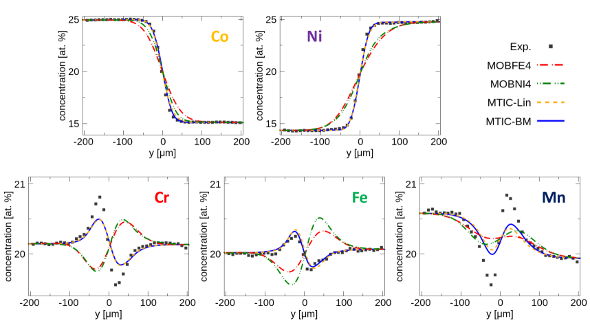
Figure 6: Comparison between experimentally obtained interdiffusion profiles and simulated ones using the HEA-DB Haase2017 combined with different atomic mobility databases (compare Fig. 5) for all five elements (Co, Cr, Fe, Mn and Ni) after 48 h at 1373 K.

IV.2.2 Comparison of atomic mobility databases to experimental results

Atomic mobilities which are directly related to the self-diffusion coefficients by the Einstein relation ($D_{i}=RTM_{i}$) and their composition dependence play a significant role in interdiffusion, see Eq. 6, and in tracer diffusion, see Eq. 13. In Fig. 5 the composition dependence of the atomic mobilities from different sources is presented with respect to the variation of the Co/Ni concentration. Cr, Fe and Mn concentrations are assumed to be constant ($20$ at.$\,\%$) while the Co concentration is increased on the expense of Ni. This represents the simplified version of the zone with neglection of uphill diffusion.
The atomic mobilities determined using the modified tracer-interdiffusion couple (MTIC) along the interdiffusion path and shown in Fig. 3 are represented by blue crosses. To convert it into a function only depending on the Co/Ni concentration, the result was averaged over the Co concentration (assuming the deviations of Cr, Fe and Mn from $20$ at.$\,\%$ are negligible). The tracer volume diffusion coefficients listed in Table 1 for Co₂₅CrFeMnNi₁₅ and Co₁₅CrFeMnNi₂₅ are shown by grey squares. To obtain a continuous composition dependence, they were linearly interpolated along the diffusion path (grey solid line).
For Co the atomic mobilities are highest obtained from MOBNI4 database and they are decreasing with increasing Co concentration. Atomic mobilities from MOBFE4 database are the lowest ones and those ones determined from the experiments are in between. For Cr the atomic mobilities from MOBFE4 and MOBNI4 are similar to each other and smaller than those ones obtained from the experiments. The same accounts for the atomic mobility of Fe, but in this case the databases offer higher values than those ones determined from the experiments. In case of Mn the atomic mobilities from MOBNI4 are higher than those ones from MOBFE4. Again the experimentally determined atomic mobilities are intermediate.
Ni tracer diffusion was not measured in the combined tracer and interdiffusion experiment, but there are data for the equiatomic alloy (only tracer) at the same temperature. Since the composition dependence of the Ni tracer diffusion coefficient was not evaluated, it is taken in the following simulations as a constant. A comparison of the measured Ni tracer diffusion coefficient in the equiatomic alloy to the data from the MOBNI4 and MOBFE4 database is also shown in Table 3. In both databases Ni diffusion is predicted as one order of magnitude faster than it is measured in the equiatomic alloy.

Table 3: Comparison of Ni self-diffusion coefficients in equiatomic CoCrFeMnNi at 1373 K.

Source	D* ($10^{-15}$ m2s-1)
MOBNI4	9.54
MOBFE4	10.50
Experiment	0.83

IV.2.3 Influence of the atomic mobilities on the interdiffusion profiles

For the following simulations only HEA-DB Haase2017 is considered for thermodynamics and combined with the different CALPHAD-type kinetic databases (MOBFE4 and MOBNI4) and the new kinetic databases (MTIC-Lin and MTIC-BM) determined from experiments. For MTIC-Lin and MTIC-BM the Ni diffusivity is taken as constant ($D^{*}_{\text{Ni}}=$ 8.34$\times$10^-16 m²s^-1) determined from the tracer diffusion experiment in the equiatomic sample. The resulting interdiffusion profiles are shown in Fig. 6.

Co
In case of Co the MOBNI4 database provides the highest atomic mobilities while the MOBFE4 database gave the smallest ones. The atomic mobilities obtained from the experiments were in between (compare Fig. 5). The simulated diffusion profiles do not represent this order. Both simulations using the atomic mobilities from the databases were significantly faster than the experiment. Using the atomic mobilities determined with the MTIC approach (MTIC-Lin and MTIC-BM data repository), both reproduce the experimental result very well. This highlights that the resulting Co interdiffusion profile is significantly influenced by the mobilities of the other elements. We highlight that exactly such cross-correlations are inherent for the new ansatz proposed in the present paper, Eq. 8.

Ni
The largest deviations between the atomic mobilities from the databases and the experiment were found for Ni, see Table 3 and Fig. 5, which is reflected in the final Ni interdiffusion profile. Using the kinetics from the databases (MOBFE4 and MOBNI4) results in significantly flatter profiles than the experimentally measured one, while using the Ni self-diffusion coefficient as a constant, obtained from the tracer experiment in the equiatomic alloy, reproduces it very well, Fig. 5.

Cr, Fe and Mn
Applying the MTIC-Lin, as well as the MTIC-BM kinetic data, uphill diffusion for Cr and Fe reverts compared to the profiles obtained using the CALPHAD-type databases. For Cr the measured diffusivities (MTIC-Lin and MTIC-BM) are slightly higher than those ones from the databases, and for Fe it is the other way around. Because this inversion can only be seen when Ni is slowed down, the cross effects with Ni play a key role for diffusion of Cr and Fe.
For Mn the uphill diffusion is in the same direction as in the experiment although it is not as distinct as in the experiment. Using the MTIC-BM approach gives a slightly better result than using MTIC-Lin.

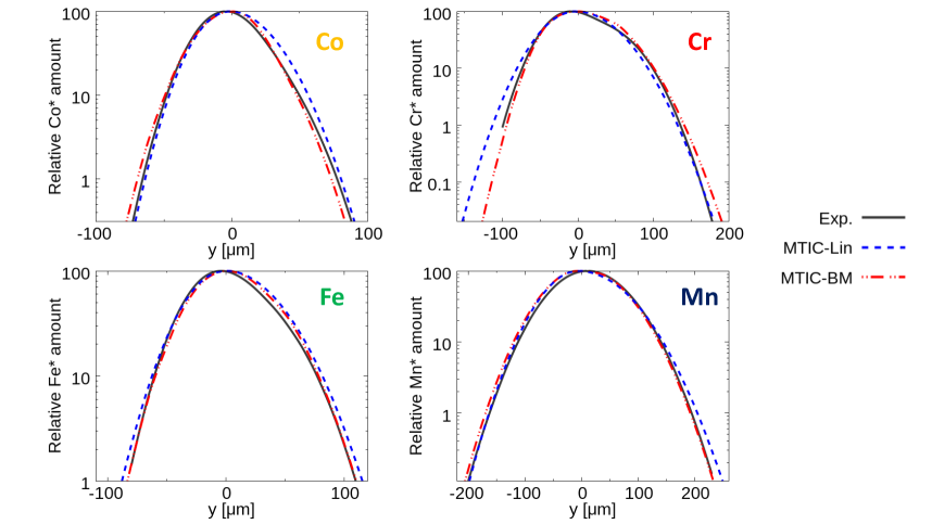
Figure 7: Comparison between experimentally obtained tracer profiles and simulated ones in the interdiffusion zone. The thermodynamic database HEA-DB was used and combined with two different composition dependent atomic mobility data repositories: MTIC-Lin and MTIC-BM (compare section IV.1.1 - Atomic mobility $M_{i}$).

IV.2.4 Tracer diffusion simulations

It was shown in the previous section that the measured self-diffusion coefficients in this work play a key role for the interdiffusion profiles. The advantage of the combined tracer-interdiffusion experiment is not only the determination of the composition dependent self-diffusion coefficients but also the measured tracer profiles that can be compared to the simulated ones.
The experimental and simulated tracer profiles in the interdiffusion zone are shown in Fig. 7. The results are given for the thermodynamic database HEA-DB combined with the atomic mobilities from MTIC-Lin and MTIC-BM. For all four elements the differences between the curves are small. For Co and Fe the whole profile is better represented using the MTIC-BM data repository. For Cr the Ni rich (right) side is better reproduced using MTIC-Lin, while the Co rich (left) side is better with MTIC-BM. For Mn the Co rich (left) side is slightly better using MTIC-Lin while the Ni rich (right) side is perfectly represented using MTIC-BM.

V Summary

In the present work, the concentration dependent tracer diffusion coefficients and the tracer diffusion coefficients of the unaffected end-members were determined for the first time using a modified tracer-interdiffusion couple approach. All the unaffected end-member tracer diffusion coefficients increase up to $75\,\%$ with decreasing Co-concentration along the diffusion path. The concentration dependent tracer diffusion coefficient of Co was found to follow a non-monotonous behaviour, which is influenced by the up-hill diffusion of Mn. The end-member diffusion coefficients of Co, Fe and Mn are in a good agreement with the determined trends for intermediate concentrations, while Cr shows larger deviations.
Based on the experimentally determined atomic mobilities, the prediction of the experimental results by diffusion simulations using a new ansatz for the generalized diffusion model is more exact than using other existing kinetic databases. Using the experimental results of the modified tracer-interdiffusion couple (MTIC) as the mobility database and the thermodynamic database by Bengt-Hallstedt (HEA-DB) - which was developed for the given near-equiatomic compositions - the simulations predict the interdiffusion-profiles as well as the tracer-profiles very well. For the elements without an initial concentration gradient the direction of the up-hill diffusion agrees perfectly with the experiment when the MTIC-Lin or MTIC-BM results are used, while it is reverse if the existing databases with Fe or Ni as the reference element are applied.
Accounting for significantly different scales on which tracer and chemical diffusion near the Matano plane could be followed, Fig. 2, we conclude that the concept of ’sluggish’ diffusion - if at all - may be applicable for the description of chemical instabilities in HEAs, but definitely not for tracer diffusion in these alloys.

Appendix A - Derivation of the pair-wise diffusion model

In a multi-component system the following relations are given and used in this derivation: $x_{j}=c_{j}V_{m}$, $V_{m}=\sum_{j=1}^{n}x_{j}\tilde{V}_{j}$, $\sum_{j=1}^{n}\tilde{V}_{j}c_{j}=1$, $\sum_{j=1}^{n}\tilde{V}_{j}dc_{j}=0$ and the Gibbs-Duhem relation ($V_{m}$ is the molare volume and $\tilde{V}_{j}$ the partial molare volume with respect to element $j$).
Starting from the mass conservation equations as in Boettinger2016 :

$$\frac{\partial c_{j}}{\partial t}+\nabla J_{j}+\nabla(c_{j}*v) =0$$ (A1)

and replacing the velocity by:

$$\nabla v=-\sum_{i=1}^{n}\nabla J_{j}V_{j}$$ (A3)

results in:

$$\frac{\partial c_{j}}{\partial t}=-\nabla\sum_{\begin{subarray}{c}i=1\\ i\neq j\end{subarray}}^{n}V_{i}c_{i}J_{j}+\nabla(c_{j}\sum_{\begin{subarray}{c}i=1\\ i\neq j\end{subarray}}^{n}J_{i}V_{i})$$ (A4)

Inserting the intrinsic flux $J_{i}=-\widehat{M}_{i}c_{i}\frac{\partial\mu_{i}}{\partial_{z}}$ and making use of the Gibbs-Duhem equation:

$$\frac{\partial c_{j}}{\partial t}=-\nabla\sum_{\begin{subarray}{c}i=1\\ i\neq j\end{subarray}}^{n}\bigg{[}\sum_{\begin{subarray}{c}k=1\\ k\neq j\end{subarray}}^{n}c_{i}c_{k}\widehat{M}_{j}V_{k}\nabla\mu_{i}+c_{i}c_{j}\widehat{M}_{i}V_{i}\nabla\mu_{i}\bigg{]}$$ (A5)

Multiply by $1=\sum_{i=1}^{n}x_{i}=V_{m}\sum_{i=1}^{n}c_{i}$:

$$\frac{1}{V_{m}}\frac{\partial c_{j}}{\partial t} = -\nabla\sum_{\begin{subarray}{c}i=1\\ i\neq j\end{subarray}}^{n}\bigg{[}\sum_{\begin{subarray}{c}k=1\\ k\neq j\end{subarray}}^{n}c_{i}c_{k}\widehat{M}_{j}V_{k}\nabla\mu_{i}+c_{i}c_{j}\widehat{M}_{i}V_{i}\nabla\mu_{i}\bigg{]}\times$$ (A6)

$$\sum_{l=1}^{n}c_{l}$$

Finally rewrite this term into pair-interactions:

$$\frac{\partial x_{j}}{\partial t} = \frac{1}{V_{m}}\nabla\sum_{\begin{subarray}{c}i=1\\ i\neq j\end{subarray}}^{n}\bigg{[}\bigg{(}\sum_{\begin{subarray}{c}k=1\\ k\neq j\\ k\neq i\end{subarray}}^{n}x_{i}x_{j}x_{k}(\widehat{M}_{i}V_{i}-\widehat{M}_{k}V_{k}+\widehat{M}_{j}V_{k})$$ (A7)

$$+ x_{i}x_{j}(x_{i}\widehat{M}_{j}V_{i}+x_{j}\widehat{M}_{i}V_{i})\bigg{)}\nabla(\mu_{j}-\mu_{i})\bigg{]}$$

Assume $V_{i}=V_{j}=V_{k}=V_{m}$:

$$\frac{\partial x_{j}}{\partial t} = \nabla\sum_{\begin{subarray}{c}i=1\\ i\neq j\end{subarray}}^{n}\bigg{[}x_{i}x_{j}\bigg{(}x_{i}\widehat{M}_{j}+x_{j}\widehat{M}_{i}+$$ (A8)

$$\sum_{\begin{subarray}{c}k=1\\ k\neq j\\ k\neq i\end{subarray}}^{n}x_{k}(\widehat{M}_{i}+\widehat{M}_{j}-\widehat{M}_{k})\bigg{)}\nabla(\mu_{j}-\mu_{i})\bigg{]}$$

Finally we introduce a factor 1/2, $M_{i}$ = $\frac{1}{2}\widehat{M}_{i}$, for model consistency with experimental data in the dilute limit (compare Appendix B):

$$\frac{\partial x_{j}}{\partial t} = \frac{1}{2}\nabla\sum_{\begin{subarray}{c}i=1\\ i\neq j\end{subarray}}^{n}\bigg{[}x_{i}x_{j}\bigg{(}x_{i}M_{j}+x_{j}M_{i}+$$ (A9)

$$\sum_{\begin{subarray}{c}k=1\\ k\neq j\\ k\neq i\end{subarray}}^{n}x_{k}(M_{i}+M_{j}-M_{k})\bigg{)}\nabla(\mu_{j}-\mu_{i})\bigg{]}$$

Appendix B - Dilute solution limit of pair-wise diffusion model

For simplification the Gibbs energy is given by an ideal solution model:

$$G^{\text{ideal}} =\sum_{i=1}^{n}x_{i}G_{i}(T)-TS^{\text{ideal}}$$ (B1)

$$=\sum_{i=1}^{n}x_{i}G_{i}(T)+RT\sum_{i=1}^{n}x_{i}\ln{(x_{i})}$$ (B2)

The derivatives of the chemical potentials with respect to site fractions are given as $\frac{\partial\mu_{j}}{\partial x_{j}}=\frac{RT}{x_{j}}$ and $\frac{\partial\mu_{j}}{\partial x_{k}}=-\frac{RT}{x_{j}}$.
Rewriting the diffusion equation depending on the concentration gradient:

$$\frac{\partial x_{j}}{\partial t} = \frac{1}{2}\nabla\sum_{\begin{subarray}{c}i=1\\ i\neq j\end{subarray}}^{n}\bigg{[}\bigg{(}\sum_{\begin{subarray}{c}k=1\\ k\neq j\\ k\neq i\end{subarray}}^{n}x_{i}x_{j}x_{k}(M_{i}+M_{j}-M_{k})+$$ (B3)

$$x_{i}x_{j}(x_{i}M_{j}+x_{j}M_{i})\bigg{)}\sum_{l=1}^{n}\bigg{(}\frac{\partial\mu_{j}}{\partial x_{l}}-\frac{\partial\mu_{i}}{\partial x_{l}}\bigg{)}\nabla x_{l}\bigg{]}$$

Replacing the derivatives of the chemical potential:

$$\frac{\partial x_{j}}{\partial t} = \frac{1}{2}\nabla\sum_{\begin{subarray}{c}i=1\\ i\neq j\end{subarray}}^{n}\bigg{[}\bigg{(}\sum_{\begin{subarray}{c}k=1\\ k\neq j\\ k\neq i\end{subarray}}^{n}x_{i}x_{j}x_{k}(M_{i}+M_{j}-M_{k})+$$ (B4)

$$x_{i}x_{j}(x_{i}M_{j}+x_{j}M_{i})\bigg{)}\times$$

$$\bigg{(}\sum_{\begin{subarray}{c}l=1\\ l\neq i\\ l\neq j\end{subarray}}^{n}\bigg{(}-\frac{RT}{x_{j}}+\frac{RT}{x_{i}}\bigg{)}\nabla x_{l}+$$

$$\bigg{(}-\frac{RT}{x_{j}}-\frac{RT}{x_{i}}\bigg{)}\nabla x_{i}+$$

$$\bigg{(}\frac{RT}{x_{j}}+\frac{RT}{x_{i}}\bigg{)}\nabla x_{j}\bigg{)}\bigg{]}$$

Replace the gradient of $x_{i}$: $\nabla x_{i}=-\sum_{\begin{subarray}{c}m=1\\ m\neq i\end{subarray}}^{n}\nabla x_{m}$ and rewrite the equation:

$$\frac{\partial x_{j}}{\partial t} = RT\nabla\sum_{\begin{subarray}{c}i=1\\ i\neq j\end{subarray}}\bigg{[}\bigg{(}\sum_{\begin{subarray}{c}k=1\\ k\neq j\end{subarray}}^{n}x_{j}x_{k}M_{j}-\sum_{\begin{subarray}{c}k=1\\ k\neq j\end{subarray}}^{n}x_{j}x_{k}M_{k}+x_{j}M_{i}\bigg{)}\times$$ (B5)

$$\sum_{\begin{subarray}{c}l=1\\ l\neq i\end{subarray}}^{n}\nabla x_{l}+\bigg{(}x_{i}M_{j}-x_{j}x_{i}M_{j}+x_{j}x_{i}M_{i}\bigg{)}\nabla x_{j}\bigg{]}$$

In the dilute limit: $x_{j}\rightarrow 0$:

$$\frac{\partial x_{j}}{\partial t} =RT\nabla\sum_{\begin{subarray}{c}i=1\\ i\neq j\end{subarray}}x_{i}M_{j}\nabla x_{j}$$ (B6)

$$\frac{\partial x_{j}}{\partial t} =RT\nabla M_{j}\nabla x_{j}$$ (B7)

Note that this convention is different to the DICTRA convention by a factor of 2 (compare Eq. A9).

Appendix C - Data repositories

The composition dependent atomic mobilities (except for Ni) in the MTIC-Lin data repository are given as: (in m²Js^-1mol^-1 at $T=1373$ K)

$$M_{\text{Co}} =-7.90\times 10^{-19}+3.03\times 10^{-19}\cdot x_{\text{Co}}$$

$$M_{\text{Cr}} =-14.9\times 10^{-19}+7.15\times 10^{-19}\cdot x_{\text{Co}}$$

$$M_{\text{Fe}} =-15.8\times 10^{-19}+6.05\times 10^{-19}\cdot x_{\text{Co}}$$

$$M_{\text{Mn}} =-45.2\times 10^{-19}+18.5\times 10^{-19}\cdot x_{\text{Co}}$$

$$M_{\text{Ni}} =7.3\times 10^{-20}$$

These equations can be rewritten in the Redlich-Kister expansion compatible with the DICTRA-notation: (in Jmol^-1)
Mobility of Co:

MQ(FCC,CO:VA,0) $$=Q_{\text{Co}}^{\text{Co}}=-430713$$

MQ(FCC,CR:VA,0) $$=Q_{\text{Co}}^{\text{Cr}}=-368291$$

MQ(FCC,FE:VA,0) $$=Q_{\text{Co}}^{\text{Fe}}=-368291$$

MQ(FCC,MN:VA,0) $$=Q_{\text{Co}}^{\text{Mn}}=-368291$$

MQ(FCC,NI:VA,0) $$=Q_{\text{Co}}^{\text{Ni}}=-368291$$

Mobility of Cr:

MQ(FCC,CO:VA,0) $$=Q_{\text{Cr}}^{\text{Co}}=-360576$$

MQ(FCC,CR:VA,0) $$=Q_{\text{Cr}}^{\text{Cr}}=-400765$$

MQ(FCC,FE:VA,0) $$=Q_{\text{Cr}}^{\text{Fe}}=-360576$$

MQ(FCC,MN:VA,0) $$=Q_{\text{Cr}}^{\text{Mn}}=-360576$$

MQ(FCC,NI:VA,0) $$=Q_{\text{Cr}}^{\text{Ni}}=-360576$$

Mobility of Fe:

MQ(FCC,CO:VA,0) $$=Q_{\text{Fe}}^{\text{Co}}=-360546$$

MQ(FCC,CR:VA,0) $$=Q_{\text{Fe}}^{\text{Cr}}=-360546$$

MQ(FCC,FE:VA,0) $$=Q_{\text{Fe}}^{\text{Fe}}=-423196$$

MQ(FCC,MN:VA,0) $$=Q_{\text{Fe}}^{\text{Mn}}=-360546$$

MQ(FCC,NI:VA,0) $$=Q_{\text{Fe}}^{\text{Ni}}=-360546$$

Mobility of Mn:

MQ(FCC,CO:VA,0) $$=Q_{\text{Mn}}^{\text{Co}}=-348709$$

MQ(FCC,CR:VA,0) $$=Q_{\text{Mn}}^{\text{Cr}}=-348709$$

MQ(FCC,FE:VA,0) $$=Q_{\text{Mn}}^{\text{Fe}}=-348709$$

MQ(FCC,MN:VA,0) $$=Q_{\text{Mn}}^{\text{Mn}}=-402756$$

MQ(FCC,NI:VA,0) $$=Q_{\text{Mn}}^{\text{Ni}}=-348709$$

Mobility of Ni:

MQ(FCC,CO:VA,0) $$=Q_{\text{Ni}}^{\text{Co}}=-387994$$

MQ(FCC,CR:VA,0) $$=Q_{\text{Ni}}^{\text{Cr}}=-387994$$

MQ(FCC,FE:VA,0) $$=Q_{\text{Ni}}^{\text{Fe}}=-387994$$

MQ(FCC,MN:VA,0) $$=Q_{\text{Ni}}^{\text{Mn}}=-387994$$

MQ(FCC,NI:VA,0) $$=Q_{\text{Ni}}^{\text{Ni}}=-387994$$

References

- (1) B.S. Murty, J.W. Yeh, S. Ranganathan, High Entropy Alloys. Elsevier, London (2014).
- (2) J.W. Yeh, S.K. Chen, S.J. Lin, J.Y. Gan, T.S. Chin, T.T. Shun, C.H. Tsau, S.Y. Chang, Nanostructured high-entropy alloys with multiple principal elements: novel alloy design concepts and outcomes, Adv. Eng. Mater 6 (2004) 299-303.
- (3) F. Zhang, C. Zhang, S.K. Chen, J. Zhu, W.S. Cao, U.R. Kattner, An understanding of high entropy alloys from phase diagram calculations. Calphad 45 (2014) 1-10.
- (4) D. Ma, B. Grabowski, F. Körmann, J. Neugebauer, D. Raabe, Ab initio thermodynamics of the CoCrFeMnNi high entropy alloy: importance of entropy contributions beyond the configurational one, Acta Mater 100 (2015) 90-97.
- (5) B. Schuh, F. Mendez-Martin, B. Völker, E.P. George, H. Clemens, R. Pippan, A. Hohenwarter, Mechanical properties, microstructure and thermal stability of a nanocrystalline CoCrFeMnNi high-entropy alloy after severe plastic deformation, Acta Mater 96 (2015) 258-268.
- (6) F. Otto, A. Dlouhý, K.G. Pradeep, M. Kuběnová, D. Raabe, G. Eggeler, E.P. George, Decomposition of the single-phase high-entropy alloy CrMnFeCoNi after prolonged anneals at intermediate temperatures, Acta Mater 112, (2016) 40-52.
- (7) N.N. Guo, L. Wang, L.S. Luo, X.Z. Li, R.R. Chen, Y.Q. Su, J.J. Guo, H.Z. Fu, Hot deformation characteristics and dynamic recrystallization of the MoNbHfZrTi refractory high-entropy alloy, Mater. Sci. Eng. A 651 (2016) 698-707.
- (8) H. Chen, A. Kauffmann, B. Gorr, D. Schliephake, C. Seemüller, J.N. Wagner, H.-J. Christ, M. Heilmaier, Microstructure and mechanical properties at elevated temperatures of a new Al-containing refractory high-entropy alloy Nb-Mo-Cr-Ti-Al, J. Alloys Compd. 661 (2016) 206-215.
- (9) D.H. Lee, M.Y. Seok, Y. Zhai, I.C. Choi, J. He, Z. Lu, J.Y. Suh, U. Ramamurty, M. Kawasaki, T.G. Langdon, J.I. Jang, Spherical nanoindentation creep behavior of nanocrystalline and coarse-grained CoCrFeMnNi high-entropy alloys, Acta Mater 109 (2016) 314-322.
- (10) L. Zhang, P. Yu, H. Cheng, H. Zhang, H. Diao, Y. Shi, B. Chen, P. Chen, R. Feng, J. Bai, Q. Jing, M. Ma, P.K. Liaw, G. Li, R. Liu, Nanoindentation creep behavior of an Al0.3CoCrFeNi high-entropy alloy, Metall. Mater. Trans. A (2016) 1-5.
- (11) Y. Ma, Y.H. Feng, T.T. Debela, G.J. Peng, T.H. Zhang, Nanoindentation study on the creep characteristics of high-entropy alloy films: fcc versus bcc structures, Int. J. Refract. Met. H. 54 (2016) 395-400.
- (12) T. Cao, J. Shang, J. Zhao, C. Cheng, R. Wang, H. Wang, The influence of Al elements on the structure and the creep behavior of AlxCoCrFeNi high entropy alloys, Mater. Lett. 164 (2016) 344-347.
- (13) W. Kai, C.C. Li, F.P. Cheng, K.P. Chu, R.T. Huang, L.W. Tsay, J.J. Kai, The oxidation behavior of an equimolar FeCoNiCrMn high-entropy alloy at 950 ∘C in various oxygen-containing atmospheres, Corros. Sci. 108 (2016) 209-214.
- (14) G. Laplanche, U.F. Volkert, G. Eggeler, E.P. George, Oxidation behavior of the CrMnFeCoNi high-entropy alloy, Oxid. Met. 85 (2016) 629-645.
- (15) G.R. Holcomb, J. Tylczak, C. Carney, Oxidation of CoCrFeMnNi high entropy alloys, JOM 67 (2015) 2326-2339.
- (16) R.A. Shaginyan, N.A. Krapivka, S.A. Firstov, N.I. Danilenko, I.V. Serdyuk, Superhard vacuum coatings based on high-entropy alloys, Powder Metall. Met. C+ 54 (2016) 725-730.
- (17) E.J. Pickering, N.G. Jones, High-entropy alloys: a critical assessment of their founding principles and future prospects, Int. Mater. Rev. (2016) 1-20.
- (18) D.B. Miracle: High-entropy alloys, A current evaluation of founding ideas and core effects and exploring "nonlinear alloys", JOM 69 (2017) 2130-2136.
- (19) S. Praveen, J. Basu, S, Kashyap, R.S. Kottada, Exceptional resistance to grain growth in nanocrystalline CoCrFeNi high entropy alloy at high homologous temperatures, J. Alloys Compd. 662 (2016) 361-367.
- (20) K.Y. Tsai, M.H. Tsai, J.W. Yeh, Sluggish diffusion in Co-Cr-Fe-Mn-Ni high-entropy alloys, Acta Mater 61 (2013) 4887-4897.
- (21) K. Kulkarni, G.P.S. Chauhan, Investigations of quaternary interdiffusion in a constituent system of high entropy alloys, AIP Adv. 5 (2015) 097162.
- (22) J. Dabrowa, W. Kucza, G. Cieslak, T. Kulik, M. Danielewski, J.W. Yeh, Interdiffusion in the FCC-structured Al-Co-Cr-Fe-Ni high entropy alloys: experimental studies and numerical simulations, J. Alloys Compd. 674 (2016) 455-462.
- (23) M. Vaidya, S. Trubel, B.S. Murty, G. Wilde, S.V. Divinski, Ni tracer diffusion in CoCrFeNi and CoCrFeMnNi high entropy alloys, JALCOM 688 (2016) 994-1001.
- (24) M. Vaidya, K.G. Pradeep, B.S. Murty, G. Wilde, S.V. Divinski, Radioactive isotopes reveal a non sluggish kinetics of grain boundary diffusion in high entropy alloys, Scientific Reports 7 (2017) 12273.
- (25) M. Vaidya, K.G. Pradeep, B.S. Murty, G. Wilde, S.V. Divinski, Bulk tracer diffusion in CoCrFeNi and CoCrFeMnNi high entropy alloys, Acta Mater 146 (2018) 211-224.
- (26) D. Gaertner, J. Kottke, Y. Chumlyakov, G. Wilde, S.V. Divinski, Tracer diffusion in single crystalline CoCrFeNi and CoCrFeMnNi high entropy alloys, JMR (2018) in press.
- (27) W. J. Boettinger, J.E. Guyer, C.E. Campbell, G.B. McFadden, Computation of the Kirkendall velocity and displacement fields in a one-dimensional binary diffusion couple with a moving interface, Proc. R. Soc. A 463 (2007) 3347-3373.
- (28) Q. Chen, A. Engström, J. Ågren, On Negative Diagonal Elements in the Diffusion Coefficient Matrix of Multicomponent Systems, J. Phase Equilib. Diffus. 39 (2018) 592-596.
- (29) A. Paul, A pseudobinary approach to study interdiffusion and the Kirkendall effect in multicomponent systems, Philos. Mag. 93 (2013) 2297-2315.
- (30) T.R. Paul, I.V. Belova, G.E. Murch, Analysis of diffusion in high entropy alloys, Mater. Chem. Phys. 210 (2017) 301-308.
- (31) S.V. Divinski, A. Pokoev, N. Eesakkiraja, A. Paul, A mystery of ’sluggish diffusion’ in high-entropy alloys: the truth or a myth?, Diffusion Foundations (2018) accepted.
- (32) M. Vaidya, M. Muralikrishna, S.V. Divinski, B.S. Murty, Non-sluggish interdiffusion kinetics in CoCrFeNi and CoCrFeMnNi high entropy alloys at elevated temperature, Scripta Mater 157 (2018) 81-85.
- (33) J. Ågren, Diffusion in phases with several components and sublattices, J. Phys. Chem. Solids 43 (1982) 5.
- (34) J.-O. Andersson, J. Ågren, Models for numerical treatment of multicomponent diffusion in simple phases, J. Appl. Phys. 72 (1992) 4.
- (35) A. Borgenstam, A. Engström, L. Höglund, J. Ågren, DICTRA, a tool for simulation of diffusional transformations in alloys, J. Phase Equilibr. 21 (2009) 269.
- (36) L. Zhang, M. Stratmann, Y. Du, B. Sundmann, I. Steinbach, Incorporating the CALPHAD sublattice approach of ordering into the phase-field model with finite interface dissipation, Acta Mater 88 (2015) 156-159.
- (37) H. L. Lukas, S.G. Fries, B. Sundman, Computational Thermodynamics. The Calphad Method, Cambridge University Press, Cambridge (2010).
- (38) C.E. Campbell, W.J. Boettinger, U.R. Kattner, Development of a diffusion mobility database for Ni-base superalloys, Acta Mat. 50 (2002).
- (39) Thermo-Calc Software TCS High Entropy Alloys Database Version 3.
- (40) C. Haase, F. Tang, M. B. Wilms, A. Weisheit, B.Hallstedt, Combining thermodynamic modeling and 3D printing of elemental powder blends for high-throughput investigation of high-entropy alloys - Towards rapid alloy screening and design, Mater. Sci. Eng., A 688 (2017) 180-189.
- (41) Thermo-Calc Software TCS High Entropy Alloy Database and Thermo-Calc Software TCS High Entropy Alloy Mobility Database.
- (42) Thermo-Calc Software, TCNI Ni-based Superalloys Database Version 8 (accessed 4 June 2018).
- (43) H.R. Lemmer, O.J.A. Segaert, M.A. Grace, The decay of Cobalt 57, Proc. Phys. Soc. A 68 (1955) 701-708.
- (44) S. Ofer, R. Wiener, Decay of Cr 51, Phys. Rev. 107 (1957) 1639-1641.
- (45) R.L. Heath, C.W. Reich, D.G. Proctor, Decay of 45-Day Fe 59, Phys. Rev. 118 (1960) 1082.
- (46) C.M. Lederer, V.S. Shirley, Table of Isotopes, 7th ed, Wiley, New York (1978).
- (47) H. Mehrer, Diffusion in Solids: Fundamentals, Methods, Materials, Diffusion-controlled Processes, Springer, Berlin (2007).
- (48) I. Belova, Y. Sohn, G. Murch, Measurement of tracer diffusion coefficients in an interdiffusion context for multicomponent alloys, Phil. Mag. Let. 95 (2015) 416-424.
- (49) F. Sauer, V. Freise, Diffusion in binary alloys with volume change, Z. Elektrochem. 66 (1962) 353.
- (50) O. Redlich, A.T. Kister, Algebraic representation of thermodynamic properties and the classification of solutions, Ind. and Eng. Chem. 40 (1948) 345-348.
- (51) S.V. Divinski, M. Lohmann, Ch. Herzig, Ag grain bondary diffusion and segregation in Cu:Measurements in the types B and C diffusion regimes, Acta Mater 49 (2001) 249-261.
- (52) R. Kubo, The fluctuation-dissipation theorem, Rep. Prog. Phys. 29 (1966) 255-284.
- (53) Thermo-Calc Software, TCFE Steels/Fe-alloys Database Version 9 (accessed 8 December 2017).