Real-time self-adaptive deep stereo

Abstract

Deep convolutional neural networks trained end-to-end are the state-of-the-art methods to regress dense disparity maps from stereo pairs. These models, however, suffer from a notable decrease in accuracy when exposed to scenarios significantly different from the training set (e.g., real vs synthetic images, etc.). We argue that it is extremely unlikely to gather enough samples to achieve effective training/tuning in any target domain, thus making this setup impractical for many applications. Instead, we propose to perform unsupervised and continuous online adaptation of a deep stereo network, which allows for preserving its accuracy in any environment. However, this strategy is extremely computationally demanding and thus prevents real-time inference. We address this issue introducing a new lightweight, yet effective, deep stereo architecture, Modularly ADaptive Network (MADNet), and developing a Modular ADaptation (MAD) algorithm, which independently trains sub-portions of the network. By deploying MADNet together with MAD we introduce the first real-time self-adaptive deep stereo system enabling competitive performance on heterogeneous datasets. Our code is publicly available at https://github.com/CVLAB-Unibo/Real-time-self-adaptive-deep-stereo.

1 Introduction

Many key tasks in computer vision rely on the availability of dense and reliable 3D reconstructions of the sensed environment. Due to high precision, low latency and affordable costs, passive stereo has proven particularly amenable to depth estimation in both indoor and outdoor set-ups. Following the groundbreaking work by Mayer et al [21], current state-of-the-art stereo methods rely on deep convolutional neural networks (CNNs) that take as input a pair of left-right frames and directly regress a dense disparity map. In challenging real-world scenarios, like the popular KITTI benchmarks [8, 23], these networks turn out to be more effective, and sometimes faster, than traditional algorithms.

As recently highlighted in [40, 25], learnable models suffer from loss in performance when tested on unseen scenarios due to the domain shift between training and testing data - often synthetic and real, respectively. Good performance can be regained by fine-tuning on few annotated samples from the target domain. Yet, obtaining groundtruth labels requires the use of costly active sensors (e.g., LIDAR) and noise removal by expensive manual intervention or post-processing [43]. Recent works [40, 25, 46, 10, 45] proposed to overcome the need for labels with unsupervised losses that require only stereo pairs from the target domain. Although effective, these techniques are inherently limited by the number of samples available at training time. Unfortunately, for many tasks, like autonomous driving, it is unfeasible to acquire, in advance, samples from all possible deployment domains (e.g., every possible road and/or weather condition).

(a)
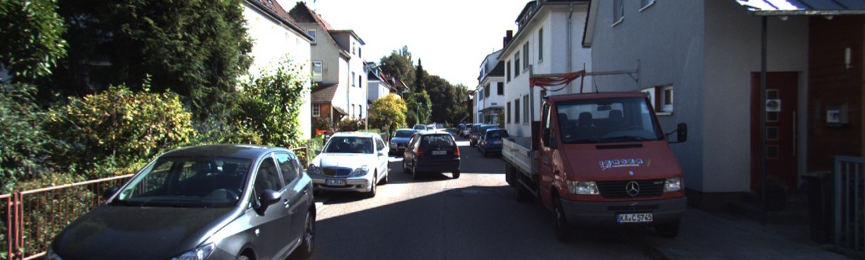
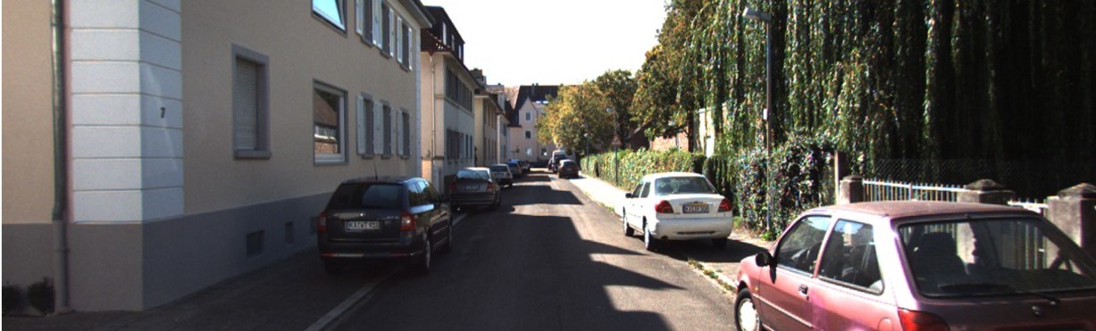
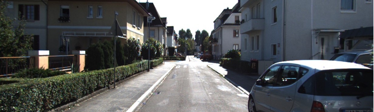
(b)
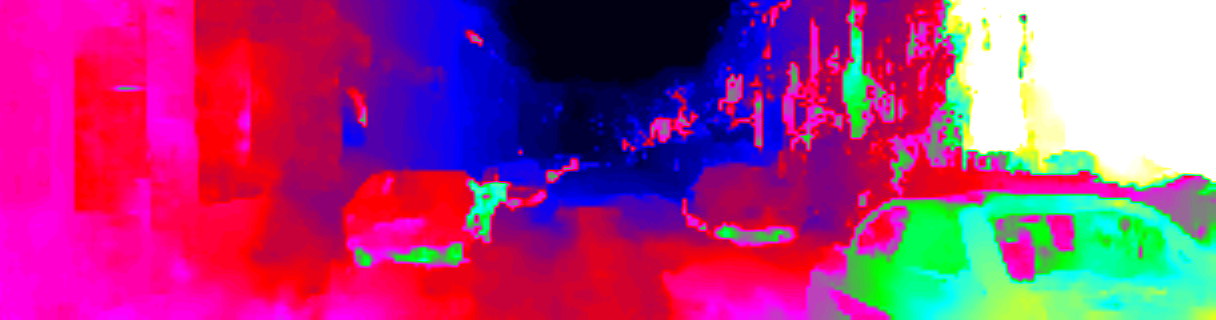
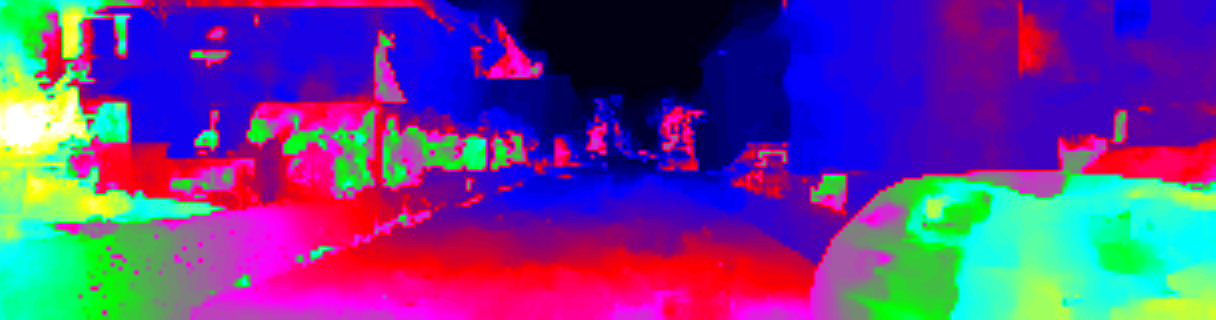
(c)
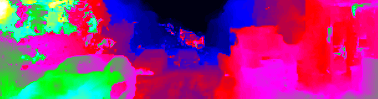
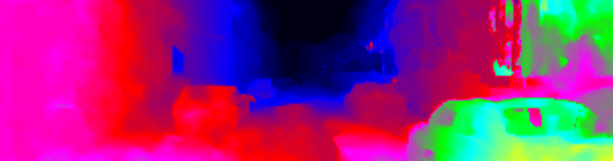
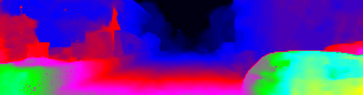
(d)
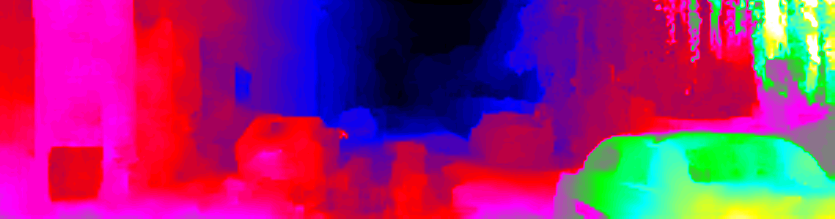
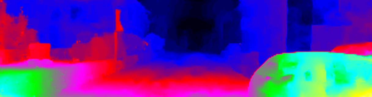
	$0^{th}$ frame	$150^{th}$ frame	$300^{th}$ frame

Figure 1: Disparity maps predicted by MADNet on a KITTI sequence [7]. Left images (a), no adaptation (b), online adaptation of the whole network (c), online adaptation by MAD (d). Green pixel values indicate larger disparities (i.e., closer objects).

We propose to address the domain shift issue by casting adaptation as a continuous learning process whereby a stereo network can evolve online based on the images gathered by the camera during its real deployment. We believe that the ability to continually adapt itself in real-time is key to any deep learning machinery intended to work in real scenarios. We achieve continuous online adaptation by: deploying one of the unsupervised losses proposed in literature (i.e., [6, 10, 40, 45]); computing error signals on the current frames; updating the whole network by back-propagation (from now on shortened as back-prop); and moving to the next pair of input frames. However, such adaptation reduces inference speed greatly. Therefore, to keep a high enough frame rate we propose a novel Modularly ADaptive Network (MADNet) architecture designed to be lightweight, fast and modular. This architecture exhibits accuracy comparable to DispNetC [21] using one-tenth parameters, runs at around $40$ FPS for disparity inference and performs an online adaptation of the whole network at around $15$ FPS. Moreover, to achieve an even higher frame rate during adaptation, at the cost of a slight loss in accuracy, we develop a Modular ADaptation (MAD) algorithm that leverages the modular architecture of MADNet in order to train sub-portions of the whole network independently. Using MADNet together with MAD we can adapt our network to unseen environments without supervision at approximately $25$ FPS.

Fig. 1 shows the disparity maps predicted by MADNet on three successive frames of a video sequence from the KITTI dataset [7]: without undergoing any adaptation - row (b); by adapting online the whole network - row (c); and by our computationally efficient MAD approach - row (d). Rows (c) and (d) show how online adaptation can improve the quality of the predicted disparity maps significantly in as few as 150 frames (i.e., a latency of about 10 seconds for complete online adaptation and 6 seconds for MAD). Extensive experimental results support our three main novel contributions:

• We cast adaptation as an online task instead of a phase prior to deployment, as previously proposed in [40, 25]. We prove that, despite a transition phase, performance of popular networks [21] with adaptation are comparable to extensive offline fine-tuning.

• We propose an extremely fast, yet accurate network for stereo matching, MADNet. Compared to the fastest model in literature [18], MADNet ranks higher on the online KITTI leader-board [23] and runs faster on the low power NVIDIA Jetson TX2. Moreover, compared to DispNetC, MADNet adapts better to unseen environments.

• We propose MAD, a novel training paradigm suited to MADNet that trades accuracy for speed and allows for significantly faster online adaptation (i.e., 25FPS). Despite this, given sufficiently long sequences, we can achieve comparable accuracy while keeping the speed advantage.

To the best of our knowledge, the synergy between MADNet and MAD realizes the first-ever real-time, self-adapting, deep stereo system.

2 Related work

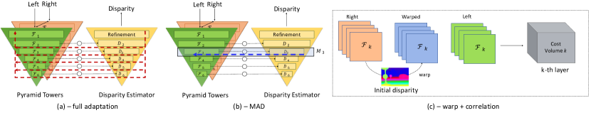
Figure 2: Sketch of MADNet architecture (a), each circle between an $F_{k}$ and $D_{k}$ represents a warp and correlation layer (c). Each pair ($\mathcal{F}_{i}$,$\mathcal{D}_{i}$) composes a module $\mathcal{M}_{i}$, adaptable independently by MAD,blue arrow in (b), faster than full back-prop, red arrow in (a).

Machine learning for stereo. Early attempts to leverage machine learning for stereo matching concerned estimating confidence measures [31], by random forest classifiers [12, 38, 26, 28] and – later – by CNNs [29, 36, 42], typically plugged into conventional pipelines to improve accuracy. CNN based matching cost functions [44, 5, 20] achieved state-of-the-art on both KITTI and Middlebury v3 by replacing conventional cost functions [14] within the SGM pipeline [13]. Eventually, Shaked and Wolf [37] proposed to rely on deep learning for both matching cost computation and disparity selection, while Gidaris and Komodakis [9] for refinement. Mayer et al [21] proposed the first end-to-end stereo architecture. Although not achieving state-of-the-art accuracy, this seminal work turned out quite disruptive compared to the traditional stereo paradigm outlined in [35], highlighting the potential for a totally new approach. Thereby, [21] ignited the spread of end-to-end stereo architectures [17, 24, 19, 4, 16, 11] that quickly outmatched any other technique on the KITTI benchmarks by leveraging on a peculiar training protocol. In particular, the deep network is initially trained on a large amount of synthetic data with groundtruth labels [21] and then fine-tuned on the target domain (e.g., KITTI) based on stereo pairs with groundtruth. All these contributions focused on accuracy, only recently Khamis et al [18] proposed a deep stereo model with a high enough frame rate to qualify for online usage at the cost of sacrificing accuracy. We will show how in our MADNet this tradeoff is more favourable. Unfortunately, all those models are particularly data dependent and their performance dramatically decay when running in environments different from those observed at training time, as shown in [40]. Batsos et al [2] soften this effect by combining traditional functions and confidence measures [15, 31] within a random forest framework, proving better generalization compared to CNN-based method [44]. Finally, guiding end-to-end CNNs with external depth measurements (e.g.Lidar) allows for reducing the domain-shift effect, as reported in [30].

Image reconstruction for unsupervised learning. A recent trend to train depth estimation networks in an unsupervised manner relies on image reconstruction losses. In particular, for monocular depth estimation this is achieved by warping different views, coming from stereo pairs or image sequences, and minimizing the reconstruction error [6, 47, 10, 45, 27, 32, 41]. This principle has also been used for optical flow [22] and stereo [46]. For the latter task, alternative unsupervised learning approaches consist in deploying traditional stereo algorithms and confidences [40] or combining by iterative optimization the predictions obtained at multiple resolutions [25]. However, we point out that both works have addressed offline training only, while we propose to solve the very same problem casting it as an online (thus fast) adaptation to unseen environments.

3 Online Domain Adaptation

Modern machine learning models reduce their accuracy when tested on data significantly different from the training set, an issue commonly referred to as domain shift. Despite all the research work to soften this issue, the most effective practice still relies on additional offline training on samples from the target environments. The domain shift curse is inherently present in deep stereo networks since most training iterations are performed on synthetic images quite different from real ones. Then, adaptation can be effectively achieved by fine-tuning the model offline on samples from the target domain by relying on expensive annotations or unsupervised loss functions [6, 10, 40, 45].

In this paper we move one step further arguing that adaptation can be effectively performed online as soon as new frames are available, thereby obtaining a deep stereo system capable of adapting itself dynamically. For our online adaptation strategy we do not rely on the availability of ground-truth annotations and, instead, use one of the proposed unsupervised losses. To adapt the model we perform on-the-fly a single train iteration (forward and backward pass) for each incoming stereo pair. Therefore, our model is always in training mode and continuously fine-tuning to the sensed environment.

3.1 MADNet - Modularly ADaptive Network

One of the main limitations that have prevented exploration of online adaptation is the computational cost of performing a full train iteration for each incoming frame. Indeed, we will show experimentally how it roughly corresponds to a reduction of the inference rate of the system to roughly one third, a price far too high to be paid with most modern architectures. To address this issue, we have developed Modularly ADaptive Network (MADNet), a novel lightweight model for depth estimation inspired by fast, yet accurate, architectures proposed for optical flow [33, 39].

We deploy a pyramidal strategy for dense disparity regression for two key purposes: i) maximizing speed and ii) obtaining a modular architecture as depicted in Fig. 2. Two pyramidal towers extract features from the left and right frames through a cascade of independent modules sharing the same weights. Each module consists of convolutional blocks aimed at reducing the input resolution by two $3\times 3$ convolutional layers, respectively with stride 2 and 1, followed by Leaky ReLU non-linearities. According to Fig. 2, we count 6 blocks providing us with feature $\mathcal{F}$ from half resolution to ${1}/{64}$, namely $\mathcal{F}_{1}$ to $\mathcal{F}_{6}$, respectively. These blocks extract 16, 32, 64, 96, 128 and 192 features.

At the lowest resolution (i.e., $\mathcal{F}_{6}$), we forward features from left and right images into a correlation layer [21] to get the raw matching costs. Then, we deploy a disparity decoder $\mathcal{D}_{6}$ consisting of 5 additional $3\times 3$ convolutional layers, with 128, 128, 96, 64, and 1 output channels. Again, each layer is followed by Leaky ReLU, except the last one, which provides the disparity map at the lowest resolution.

Then, $D_{6}$ is up-sampled to level $5$ by bilinear interpolation and used both for warping right features towards left ones before computing correlations and as input to $\mathcal{D}_{5}$. Thanks to our design, from $\mathcal{D}_{5}$ onward, the aim of the disparity decoders $\mathcal{D}_{k}$ is to refine and correct the up-scaled disparities coming from the lower resolution. In our design, the correlation scores computed between the original left and right features aligned according to the lower resolution disparity prediction guide the network in the refinement process. We compute all correlations inside our network along a [-2,2] range of possible shifts.

This process is repeated up to quarter resolution (i.e., $\mathcal{D}_{2}$), where we add a further refinement module consisting of $3\times 3$ dilated convolutions [39], with, respectively 128, 128, 128, 96, 64, 32, 1 output channels and 1, 2, 4, 8, 16, 1, 1 dilation factors, before bilinearly upsampling to full resolution. Additional details on the MADNet architecture are provided in the supplementary material.

MADNet has a smaller memory footprint and delivers disparity maps much more rapidly than other more complex networks such as [17, 4, 19] with a small loss in accuracy. Concerning efficiency, working at decimated resolutions allows for computing correlations on a small horizontal window [39], while warping features and forwarding disparity predictions across the different resolutions enables to maintain a small search range and look for residual displacements only. With a 1080Ti GPU, MADNet runs at about 40 FPS at KITTI resolution and can perform online adaptation with full back-prop at 15 FPS.

3.2 MAD - Modular ADaptation

As we will show, MADNet is remarkably accurate with full online adaptation at 15 FPS. However, for some applications, it might be desirable to achieve a higher frame rate without losing the adaptation ability. Most of the time needed to perform online adaptation is spent executing back-prop and weights update across all the network layers. A naive way to speed up the process will be to freeze the initial part of the network and fine tune only a subset of $k$ final layers, thus realizing a shorter back-prop that would yield a higher frame rate. However, there is no guarantee that these last $k$ layers are indeed those that would benefit most from online fine-tuning. For example, the initial layers of the network should be probably adapted alike, as they directly interact with the images from a new, unseen, domain. In Sec. 4.5 we will provide experimental results to show that training only the final layers is not enough for handling the drastic domain changes that typically occur in practical applications.

Following the key intuition that to keep up with fast inference we should pursue a partial, though effective, online adaptation, we developed Modular ADaptation (MAD) an online adaptation algorithm tailored to MADNet, though possibly extendable to any multi-scale inference network. Our method takes a network $\mathcal{N}$ and subdivides it into $p$ non-overlapping portions, each referred to as module $\mathcal{M}_{i}$, $i\in[1,p]$, such that $\mathcal{N}=[\mathcal{M}_{1},\mathcal{M}_{2},..\mathcal{M}_{p}]$. Each $\mathcal{M}_{i}$ ends with a final layer able to output a disparity estimation $y_{i}$. Thanks to its design, decomposing our network is straightforward by grouping layers working at the same resolution $i$ from both $\mathcal{F}_{i}$ and $\mathcal{D}_{i}$ into a single module $\mathcal{M}_{i}$, e.g., $\mathcal{M}_{3}=(\mathcal{F}_{3},\mathcal{D}_{3}$). At each training iteration, thus, we can optimize one of the modules independently from the others by using the prediction $y_{i}$ to compute a loss function and then executing the shorter back-prop only across the layers of $\mathcal{M}_{i}$. For instance to optimize $\mathcal{M}_{3}$ we would use $y_{3}$ to compute a loss function and back-prop only through $\mathcal{D}_{3}$ and $\mathcal{F}_{3}$ following the blue path in Fig. 2 (b). Conversely, full back-prop would follow the much longer red path in Fig. 2 (a). This paradigm allows for

• Interleaved optimization of different $\mathcal{M}_{i}$, thereby approximating full back-prop over time while gaining considerable speed-up.

• Fast adaptation of single modules, which instantly provides benefits to the overall accuracy of the whole network thanks to its cascade architecture.

At deployment time, for each incoming stereo pair, we run a forward pass to obtain all estimates $[y_{1},\dots,y_{p}]$ at each resolution, then we choose a portion $\theta\in[1,\dots,p]$ of the network to train according to some heuristic and finally update $\mathcal{M}_{\theta}$ according to a loss computed on $y_{\theta}$. We consider a valid heuristic any function that outputs a probability distribution among the $p$ modules of $N$ from which we could perform sampling.

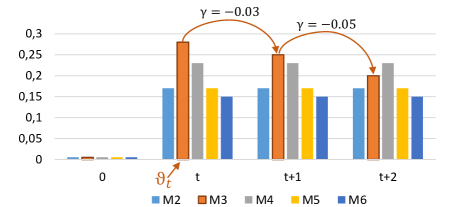
Figure 3: Example of reward/punishment mechanism. $X$ axis shows time while $Y$ histogram values. At time $t$, the most probable module selected for adaptation is $\mathcal{M}_{3}$. After two steps ($t+2$), its probability gets demoted in favour of $\mathcal{M}_{4}$.

3.3 Reward/punishment selection

Among different functions, we obtained good results using a reward/punishment mechanism. We start by creating a histogram $\mathcal{H}$ with $p$ bins (i.e., one per module) all initialized to 0. For each stereo pair we perform a forward pass to get the disparity predictions $y_{i}$ and measure the performance of the model by computing a loss $\mathcal{L}_{t}$ using the full resolution disparity $y$ and the input frames $x$ (e.g., reprojection error between left and warped right frames as in [10]). Then, we sample the portion to train $\theta\in[1,\dots,p]$ from a probability distribution obtained applying the softmax function to the value of the bins in $(\mathcal{H})$:

$$\theta_{t}\sim softmax(\mathcal{H}).$$ (1)

We can compute one optimization step for layers of $\mathcal{M}_{\theta_{t}}$ with respect to the loss $\mathcal{L}^{\theta_{t}}_{t}$ computed on the lower scale prediction $y_{\theta_{t}}$. We have now partially adapted the network to the current environment. At the following iteration, we update $\mathcal{H}$ before choosing the new $\theta_{t}$, increasing the probability of being sampled for the $\mathcal{M}_{\theta_{t-1}}$ that have proven effective. To do so we compute a noisy expected value for $\mathcal{L}_{t}$ by linear extrapolation of the losses at the previous two-time steps

$$\mathcal{L}_{exp}=2\cdot\mathcal{L}_{t-1}-\mathcal{L}_{t-2},$$ (2)

and quantify the effectiveness of the last module optimized as

$$\gamma=\mathcal{L}_{exp}-\mathcal{L}_{t}.$$ (3)

Finally, we can change the value of $\mathcal{H}[\theta_{t}]$ according to $\gamma$, i.e. effective adaptation will have $\mathcal{L}_{exp}>\mathcal{L}_{t}$, thus $\gamma>0$. We found out that adding a temporal decay to $\mathcal{H}$ increases the stability of the system, leading to the following update rule

$$\begin{split}\mathcal{H}&=0.99\cdot\mathcal{H}\\ \mathcal{H}[\theta_{t-1}]&=\mathcal{H}[\theta_{t-1}]+0.01\cdot\gamma\end{split}$$ (4)

Additional pseudo code to detail this heuristic is available in the supplementary material.

Fig. 3 shows an example of histogram $\mathcal{H}$ at generic time frames $t$ and $t+2$, highlighting the transition from $\mathcal{M}_{3}$ to $\mathcal{M}_{4}$ as most probable module thanks to the aforementioned mechanism.

4 Experimental results

4.1 Evaluation protocol and implementation

To properly address practical deployment scenarios in which there are no ground-truth data available for fine-tuning in the actual testing environments, we train our stereo network using synthetic data only [21]. More details regarding the training process can be found in the supplementary material.

To test the online adaptation we use those weights as a common initialization and carry out an extensive evaluation on the large and heterogeneous KITTI raw dataset [7] with depth labels [43] converted into disparities by knowing the camera parameters. Overall, we assess the effectiveness of our proposal on 43k images. Specifically, according to the KITTI classification, we evaluate our framework in four heterogeneous environments, namely Road, Residential, Campus and City, obtained by concatenation of the available video sequences and resulting in 5674, 28067, 1149 and 8027 frames respectively. Although these sequences are all concerned with driving scenarios, each has peculiar traits that would lead deep stereo model to gross errors without suitable fine-tuning in the target domain. For example, City and Residential often depict road surrounded by buildings, while Road concerns mostly highways and country roads, where the most common objects are cars and vegetation.

By processing stereo pairs within sequences, we can measure how well the network adapts, by either full back-prop or MAD, to the target domain compared to a model trained offline. For all experiments, we analyze both average End Point Error (EPE) and the percentage of pixels with disparity error larger than 3 (D1-all). Due to the image format being different for each sequence, we extract a central crop of size $320\times 1216$ from each frame, which suits to the downsampling factor of our architecture and allows for validating almost all pixels with available ground-truth disparities.

Finally, we highlight that for both full back-prop and MAD, we compute the error rate on each frame before applying the model adaptation step. That is, we measure performances achieved by the current model on the stereo frame at time $t$ and then adapt it according to the current prediction. Therefore, the model update carried out at time $t$ will affect the prediction only from frame $t+1$ and so on. As unsupervised loss for online adaptation, we rely on the photometric consistency between the left frame and the right one reprojected according to the predicted disparity. Following [10], to compute the reprojection error between the two images we combine the Structural Similarity Measure (SSIM) and the L1 distance, weighted by 0.85 and 0.15, respectively. We selected this unsupervised loss function as it is the fastest to compute among those proposed in literature [40, 25, 46] and does not require any additional information besides a pair of stereo images. Further details are available in the supplementary material.

4.2 MADNet performance

Before assessing the performance obtainable through online adaptation, we test the effectiveness of MADNet by following the canonic two-phase training using synthetic [21] and real data. Thus, after training on synthetic data, we perform fine-tuning on the training sets of KITTI 2012 and KITTI 2015 and submit to the KITTI 2015 online benchmark. Additional details on the fine-tuning protocol are provided in the supplementary material. On Tab. 1 we report our result compared to other (published) fast inference architectures on the leaderboard (runtime measured on NVIDIA 1080Ti) as well as with a slower and more accurate one, GWCNet [11]. At the time of writing, our method ranks 90^th. Despite the mid-rank achieved in terms of absolute accuracy, MADNet compares favorably to StereoNet [18] ranked 92^nd, the only other high frame rate proposal on the KITTI leaderboard. Moreover, we get close to the performance of the original DispNetC [21] while using $\frac{1}{10}$ of the parameters and running more than twice faster.

	GWCNet [11]	DispNetC [21]	StereoNet [18]	MADNet
D1-all	2.11	4.34	4.83	4.66
Time	0.32	0.06	0.02	0.02

Table 1: Comparison between stereo architectures on the KITTI 2015 test set without adaptation. Detailed results available in the KITTI online leader-board.

4.3 Online adaptation

		City		Residential		Campus		Road
Model	Adapt.	D1-all(%)	EPE	D1-all(%)	EPE	D1-all(%)	EPE	D1-all(%)	EPE	FPS
DispNetC	No	8.31	1.49	8.72	1.55	15.63	2.14	10.76	1.75	15.85
DispNetC	Full	4.34	1.16	3.60	1.04	8.66	1.53	3.83	1.08	5.22
DispNetC-GT	No	3.78	1.19	4.71	1.23	8.42	1.62	3.25	1.07	15.85
MADNet	No	37.42	9.96	37.41	11.34	51.98	11.94	47.45	15.71	39.48
MADNet	Full	2.63	1.03	2.44	0.96	8.91	1.76	2.33	1.03	14.26
MADNet	MAD	5.82	1.51	3.96	1.31	23.40	4.89	7.02	2.03	25.43
MADNet-GT	No	2.21	0.80	2.80	0.91	6.77	1.32	1.75	0.83	39.48

Table 2: Performance on the City, Residential, Campus and Road sequences from KITTI [7]. Experiments with DispNetC [21] (top) and MADNet (bottom) with and without online adaptations. -GT variants are fine-tuned on KITTI training set groundtruth.

We will now show how online adaptation is an effective paradigm, comparable, or better, to offline fine-tuning. Tab. 2 reports extensive experiments on the four different KITTI environments. We report results achieved by i) DispNetC [21] implemented in our framework and trained, from top to bottom, on synthetic data following authors’ guidelines, using online adaptation or fine-tuned on groundtruth and ii) MADNet trained with the same modalities and, also, using MAD. These experiments, together to Sec. 4.2, support the three-fold claim of this work.

DispNetC: Full adaptation. On top of Tab. 2, focusing on the D1-all metric, we can notice how running full back-prop online to adapt DispNetC [21] decimates the number of outliers on all scenarios compared to the model trained on the synthetic dataset only. In particular, this approach can consistently halve D1-all on Campus, Residential and City and nearly reduce it to one third on Road. Alike, the average EPE drops significantly across the four considered environments, with improvement as high as a nearly $40\%$ relative improvement on the Road sequences. These massive gains in accuracy, though, come at the price of slowing the network down significantly to about one-third of the original inference rate, i.e. from nearly 16 to 5.22 FPS. As mentioned above, the Table also reports the performance of the models fine-tuned offline on the 400 stereo pairs with groundtruth disparities from the KITTI 2012 and 2015 training dataset [23, 8]. It is worth pointing out how online adaptation by full back-prop turns out competitive to fine-tuning offline by groundtruth, and even more accurate in the Residential environment. This fact may hint at training usupervisedly by a more considerable amount of data possibly delivering better models than supervision by fewer data.

MADNet: Full adaptation. On bottom of Tab. 2 we repeat the aforementioned experiments for MADNet. Due to the much higher errors yielded by the model trained on synthetic data only, full online adaptation turns out even more beneficial with MADNet, leading to a model which is more accurate than DispNetC with Full adaptation in all sequences but Campus and can run nearly three times faster (i.e. at 14.26 FPS compared to the 5.22 FPS of DispNetC-Full). These results also highlight the inherent effectiveness of the proposed MADNet. Indeed, as vouched by the rows dealing with MADNet-GT and DispNetC-GT, using for both our implementations and training them following the same standard procedure in the field (i.e., pretraining on synthetic data and fine-tuning on KITTI training sets), MADNet yields better accuracy than DispNetC while running about 2.5 times faster.

MADNet: MAD. Once proved that online adaptation is feasible and beneficial, we show that MADNet employing MAD for adaptation (marked as MAD in column Adapt.) allows for effective and efficient adaptation. Since the proposed heuristic has a non-deterministic sampling step, we have run the tests regarding MAD five times each and reported here the average performance. We refer the reader to Sec. 4.5 for analysis on the standard deviation across different runs. Indeed, MAD provides a significant improvement in all the performance figures reported in the table compared to the corresponding models trained by synthetic data only. Using MAD, MADNet can be adapted paying a relatively small computational overhead which results in a remarkably fast inference rate of about 25 FPS. Overall, these results highlight how, whenever one has no access to training data from the target domain beforehand, online adaptation is feasible and worth. Moreover, if speed is a concern MADNet combined with MAD provides a favourable trade-off between accuracy and efficiency.

Short-term Adaptation. Tab. 2 also shows how all adapted models perform significantly worse on Campus compared the other sequences. We ascribe this mainly to Campus featuring fewer frames (1149) compared the other sequences (5674, 28067, 8027), which implies a correspondingly lower number of adaptation steps executed online. Indeed, a key trait of online adaptation is the capability to improve performance as more and more frames are sensed from the environment. This favourable behaviour, not captured by the average error metrics reported in Tab. 2, is highlighted in Fig. 4, which plots the D1-all error rate over time for MADNet models in the four modalities. While without adaptation the error keeps being always large, models adapted online clearly improve over time such that, after a certain delay, they become as accurate as the model that could have been obtained by offline fine-tuning had groundtruth disparities been available. In particular, full online adaptation achieves performance comparable to fine-tuning by the groundtruth after 900 frames (i.e., about 1 minute) while for MAD it takes about 1600 frames (i.e., 64 seconds) to reach an almost equivalent performance level while providing a substantially higher inference rate ($\sim 25$ vs $\sim 15$).

Long-term Adaptation. As Fig. 4 hints, online adaptation delivers better performance processing a higher number of frames. In Tab. 3 we report additional results obtained by concatenating together the four environments without network resets to simulate a stereo camera traveling across different scenarios for $\sim 43000$ frames. Firstly, Tab. 3 shows how both DispNetC and MADNet models adapted online by full back-prop yield much smaller average errors than in Tab. 2, as small, indeed, as to outperform the corresponding models fine-tuned offline by groundtruth labels. Hence, performing online adaptation through long enough sequences, even across different environments, can lead to more accurate models than offline fine-tuning on few samples with groundtruth, which further highlights the great potential of our proposed continuous learning formulation. Moreover, when leveraging on MAD for the sake of run-time efficiency, MADNet attains larger accuracy gains through continuous learning than before (Tab. 3 vs. Tab. 2) shrinking the performance gap between MAD and Full back-prop. We believe that this observation confirms the results plotted in Fig. 4: MAD needs more frame to adapt the network to a new environment, but given sequences long enough can successfully approximate full back propagation over time (i.e., 0.20 EPE difference and 1.2 D1-all between the two adaptation modalities on Tab. 3) while granting nearly twice FPS. On long term (e.g., beyond 1500 frames on Fig. 4) running MAD, full adaptation or offline tuning on groundtruth grants equivalent performance. Besides Fig. 1, we report qualitative results in the supplementary material as two video sequences regarding outdoor [7] and indoor [1] environments.

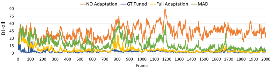
Figure 4: MADNet: error across frames in the 2011_09_30_drive_0028_sync sequence (KITTI dataset, Residential environment).

Model Adapt. D1-all(%) EPE FPS DispNetC No 9.09 1.58 15.85 DispNetC Full 3.45 1.04 5.22 DispNetC-GT No 4.40 1.21 15.85 MADNet No 38.84 11.65 39.48 MADNet Full 2.17 0.91 14.26 MADNet MAD 3.37 1.11 25.43 MADNet-GT No 2.67 0.89 39.48

Table 3: Results on the full KITTI raw dataset [7] (Campus $\rightarrow$ City $\rightarrow$ Residential $\rightarrow$ Road).

4.4 Additional results

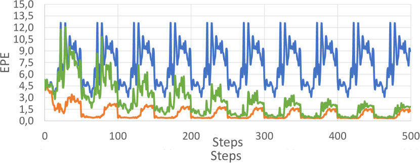
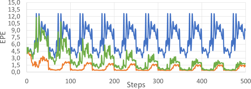
Figure 5: End-Point Error (EPE) on Middlebury Motorcycle pair (top) and Sintel Alley-2 sequence (bottom) looped over 10 times.

Here we show the generality of MAD on environments different from those depicted in the KITTI dataset. To this purpose, we run aimed experiments on the Sintel [3] and Middlebury [34] datasets and plot EPE trends for both Full and Mad adaptation on Fig. 5. This evaluation allows for measuring the performance on a short sequence concatenated multiple times (i.e., Sintel) or when adapting on the same stereo pair (i.e., Middlebury) over and over.

On Middlebury (top) we perform 300 steps of adaptation on the Motorcycle stereo pair. The plots clearly show how MAD converges to the same accuracy of Full after around 300 steps while maintaining real-time processing (25.6 FPS on image scaled to a quarter of the original resolution). On Sintel (bottom), we adapt to the Alley-2 sequence looped over 10 times. We can notice how the very few, i.e. 50, frames of the sequence are not enough to achieve good performance with MAD, since it performs the best on long-term adaptation as highlighted before. However, by looping over the same sequence, we can perceive how MAD gets closer to full adaptation, confirming the behavior already experimented on the KITTI environments.

4.5 Different online adaptation strategies

Adaptation Mode	D1-all(%)	EPE	FPS
No	38.84	11.65	39.48
Last layer	38.33	11.45	38.25
Refinement	31.89	6.55	29.82
D2+Refinement	18.84	2.87	25.85
MAD-SEQ	3.62	1.15	25.74
MAD-RAND	3.56 ($\pm 0.05$)	1.13 ($\pm 0.01$)	25.77
MAD-FULL	3.37 ($\pm 0.1$)	1.11 ($\pm 0.01$)	25.43

Table 4: Results on the KITTI raw dataset [7] using MADNet trained on synthetic data and different fast adaptation strategies

We carried out additional tests on the whole KITTI RAW dataset [7] and compared performance obtainable deploying different fast adaptation strategies for MADNet. Results are reported on Tab. 4 together with those concerning a network that does not perform any adaptation.

First, we compared MAD keeping the weights of the initial portions of the network frozen and training only: the last layer, the Refinement module or both D₂ and Refinement modules. Then, since MAD consists in splitting the network into independent portions and choosing which one to train, we compare our full proposal (MAD-FULL) to keeping the split and choosing the portion to train either randomly (MAD-RAND) or using a round-robin schedule (MAD-SEQ). Since MAD-FULL and MAD-RAND feature non-deterministic sampling steps, we report their average performance obtained across 5 independent runs on the whole dataset with the corresponding standard deviations between brackets.

By comparing the first four entries with the ones featuring MAD we can see how training only the final layers is not enough to successfully perform online adaptation. Even training as many as 13 last layers (i.e., $D_{2}+Refinement$), at a computational cost comparable with MAD, we are at most able to halve the initial error rate, with performance still far from optimal. The three variants of MAD by training the whole network can successfully reduce the D1-all to $\frac{1}{10}$ of the original. Among the three options, our proposed layer selection heuristic provides the best overall performance even taking into account the slightly higher standard deviation caused by our sampling strategy. Moreover, the computational cost to pay to deploy our heuristic is negligible losing only $0.3$ FPS compared to the other two options.

4.6 Deployment on embedded platforms

All the tests reported so far have been executed on a PC equipped with an NVIDIA 1080 Ti GPU. Unfortunately, for many application like robotics or autonomous vehicles, it is unrealistic to rely on such high end and power-hungry hardware. However, one of the key benefits of MADNet is its lightweight architecture conducive to easy deployment on low-power embedded platforms. Thus, we evaluated MADNet on an NVIDIA Jetson TX2 when processing stereo pairs at the full KITTI resolution and compared it to StereoNet [18] implemented using the same framework (i.e., the same level of optimization). We measured $0.26s$ for a single forward of MADNet versus $0.76$-$0.96s$ required by StereoNet, with 1 or 3 refinement modules respectively. Thus, for embedded applications MADNet is an appealing alternative to [18] since it is both faster and more accurate.

5 Conclusions and future work

The proposed online unsupervised fine-tuning approach can successfully tackle the domain adaptation issue for deep end-to-end disparity regression networks. We believe this to be key to practical deployment of these potentially ground-breaking deep learning systems in many relevant scenarios. For applications in which inference time is critical, we have proposed MADNet, a novel network architecture, and MAD, a strategy to effectively adapt it online very efficiently. We have shown how MADNet together with MAD can adapt to new environments by keeping a high prediction frame rate (i.e., 25FPS) and yielding better accuracy than popular alternatives like DispNetC. As main topic for future work, we plan to test and possibly extend MAD to any end-to-end stereo system. We would also like to investigate alternative approaches to select the portion of the network to be updated online at each step.

Acknowledgements. We gratefully acknowledge the support of NVIDIA Corporation with the donation of a Titan X used for this research.

blabla See pages 1 of supplementary.pdf See pages 2 of supplementary.pdf See pages 3 of supplementary.pdf See pages 4 of supplementary.pdf See pages 5 of supplementary.pdf See pages 6 of supplementary.pdf

References

- [1] Hatem Alismail, Brett Browning, and M Bernardine Dias. Evaluating pose estimation methods for stereo visual odometry on robots. In the 11th International Conference on Intelligent Autonomous Systems (IAS-11), 2011.
- [2] Konstantinos Batsos, Changjiang Cai, and Philippos Mordohai. Cbmv: A coalesced bidirectional matching volume for disparity estimation. In The IEEE Conference on Computer Vision and Pattern Recognition (CVPR), 2018.
- [3] D. J. Butler, J. Wulff, G. B. Stanley, and M. J. Black. A naturalistic open source movie for optical flow evaluation. In A. Fitzgibbon et al. (Eds.), editor, European Conf. on Computer Vision (ECCV), Part IV, LNCS 7577, pages 611–625. Springer-Verlag, Oct. 2012.
- [4] Jia-Ren Chang and Yong-Sheng Chen. Pyramid stereo matching network. In The IEEE Conference on Computer Vision and Pattern Recognition (CVPR), 2018.
- [5] Zhuoyuan Chen, Xun Sun, Liang Wang, Yinan Yu, and Chang Huang. A deep visual correspondence embedding model for stereo matching costs. In The IEEE International Conference on Computer Vision (ICCV), December 2015.
- [6] Ravi Garg, Vijay Kumar BG, Gustavo Carneiro, and Ian Reid. Unsupervised cnn for single view depth estimation: Geometry to the rescue. In European Conference on Computer Vision, pages 740–756. Springer, 2016.
- [7] Andreas Geiger, Philip Lenz, Christoph Stiller, and Raquel Urtasun. Vision meets robotics: The kitti dataset. International Journal of Robotics Research (IJRR), 2013.
- [8] Andreas Geiger, Philip Lenz, and Raquel Urtasun. Are we ready for autonomous driving? the kitti vision benchmark suite. In Computer Vision and Pattern Recognition (CVPR), 2012 IEEE Conference on, pages 3354–3361. IEEE, 2012.
- [9] Spyros Gidaris and Nikos Komodakis. Detect, replace, refine: Deep structured prediction for pixel wise labeling. In The IEEE Conference on Computer Vision and Pattern Recognition (CVPR), July 2017.
- [10] Clément Godard, Oisin Mac Aodha, and Gabriel J Brostow. Unsupervised monocular depth estimation with left-right consistency. In CVPR, volume 2, page 7, 2017.
- [11] Xiaoyang Guo, Kai Yang, Wukui Yang, Xiaoyang Wang, and Hongsheng Li. Group-wise correlation stereo network. In CVPR, 2019.
- [12] R. Haeusler, R. Nair, and D. Kondermann. Ensemble learning for confidence measures in stereo vision. In CVPR. Proceedings, pages 305–312, 2013. 1.
- [13] Heiko Hirschmuller. Accurate and efficient stereo processing by semi-global matching and mutual information. In Computer Vision and Pattern Recognition, 2005. CVPR 2005. IEEE Computer Society Conference on, volume 2, pages 807–814. IEEE, 2005.
- [14] H. Hirschmüller and D. Scharstein. Evaluation of stereo matching costs on images with radiometric differences. IEEE Transactions on Pattern Analysis and Machine Intelligence, 31:1582–1599, 08 2008.
- [15] Xiaoyan Hu and Philippos Mordohai. A quantitative evaluation of confidence measures for stereo vision. IEEE Transactions on Pattern Analysis and Machine Intelligence (PAMI), pages 2121–2133, 2012.
- [16] Zequn Jie, Pengfei Wang, Yonggen Ling, Bo Zhao, Yunchao Wei, Jiashi Feng, and Wei Liu. Left-right comparative recurrent model for stereo matching. In The IEEE Conference on Computer Vision and Pattern Recognition (CVPR), 2018.
- [17] Alex Kendall, Hayk Martirosyan, Saumitro Dasgupta, Peter Henry, Ryan Kennedy, Abraham Bachrach, and Adam Bry. End-to-end learning of geometry and context for deep stereo regression. In The IEEE International Conference on Computer Vision (ICCV), Oct 2017.
- [18] Sameh Khamis, Sean Fanello, Christoph Rhemann, Adarsh Kowdle, Julien Valentin, and Shahram Izadi. Stereonet: Guided hierarchical refinement for real-time edge-aware depth prediction. In 15th European Conference on Computer Vision (ECCV 2018), 2018.
- [19] Zhengfa Liang, Yiliu Feng, Yulan Guo Hengzhu Liu Wei Chen, and Linbo Qiao Li Zhou Jianfeng Zhang. Learning for disparity estimation through feature constancy. In The IEEE Conference on Computer Vision and Pattern Recognition (CVPR), 2018.
- [20] Wenjie Luo, Alexander G Schwing, and Raquel Urtasun. Efficient deep learning for stereo matching. In Proceedings of the IEEE Conference on Computer Vision and Pattern Recognition, pages 5695–5703, 2016.
- [21] Nikolaus Mayer, Eddy Ilg, Philip Hausser, Philipp Fischer, Daniel Cremers, Alexey Dosovitskiy, and Thomas Brox. A large dataset to train convolutional networks for disparity, optical flow, and scene flow estimation. In The IEEE Conference on Computer Vision and Pattern Recognition (CVPR), June 2016.
- [22] Simon Meister, Junhwa Hur, and Stefan Roth. UnFlow: Unsupervised learning of optical flow with a bidirectional census loss. In AAAI, New Orleans, Louisiana, Feb. 2018.
- [23] Moritz Menze and Andreas Geiger. Object scene flow for autonomous vehicles. In Conference on Computer Vision and Pattern Recognition (CVPR), 2015.
- [24] Jiahao Pang, Wenxiu Sun, Jimmy SJ. Ren, Chengxi Yang, and Qiong Yan. Cascade residual learning: A two-stage convolutional neural network for stereo matching. In The IEEE International Conference on Computer Vision (ICCV), Oct 2017.
- [25] Jiahao Pang, Wenxiu Sun, Chengxi Yang, Jimmy Ren, Ruichao Xiao, Jin Zeng, and Liang Lin. Zoom and learn: Generalizing deep stereo matching to novel domains. The IEEE Conference on Computer Vision and Pattern Recognition (CVPR), 2018.
- [26] Min Gyu Park and Kuk Jin Yoon. Leveraging stereo matching with learning-based confidence measures. In The IEEE Conference on Computer Vision and Pattern Recognition (CVPR), June 2015.
- [27] Matteo Poggi, Filippo Aleotti, Fabio Tosi, and Stefano Mattoccia. Towards real-time unsupervised monocular depth estimation on cpu. In IEEE/JRS Conference on Intelligent Robots and Systems (IROS), 2018.
- [28] Matteo Poggi and Stefano Mattoccia. Learning a general-purpose confidence measure based on o(1) features and a smarter aggregation strategy for semi global matching. In Proceedings of the 4th International Conference on 3D Vision, 3DV, 2016.
- [29] Matteo Poggi and Stefano Mattoccia. Learning from scratch a confidence measure. In Proceedings of the 27th British Conference on Machine Vision, BMVC, 2016.
- [30] Matteo Poggi, Davide Pallotti, Fabio Tosi, and Stefano Mattoccia. Guided stereo matching. In The IEEE Conference on Computer Vision and Pattern Recognition (CVPR), June 2019.
- [31] Matteo Poggi, Fabio Tosi, and Stefano Mattoccia. Quantitative evaluation of confidence measures in a machine learning world. In The IEEE International Conference on Computer Vision (ICCV), Oct 2017.
- [32] Matteo Poggi, Fabio Tosi, and Stefano Mattoccia. Learning monocular depth estimation with unsupervised trinocular assumptions. In 6th International Conference on 3D Vision (3DV), 2018.
- [33] Anurag Ranjan and Michael J. Black. Optical flow estimation using a spatial pyramid network. In The IEEE Conference on Computer Vision and Pattern Recognition (CVPR), July 2017.
- [34] Daniel Scharstein, Heiko Hirschmüller, York Kitajima, Greg Krathwohl, Nera Nesic, Xi Wang, and Porter Westling. High-resolution stereo datasets with subpixel-accurate ground truth. In Xiaoyi Jiang, Joachim Hornegger, and Reinhard Koch, editors, GCPR, volume 8753 of Lecture Notes in Computer Science, pages 31–42. Springer, 2014.
- [35] Daniel Scharstein and Richard Szeliski. A taxonomy and evaluation of dense two-frame stereo correspondence algorithms. International journal of computer vision, 47(1-3):7–42, 2002.
- [36] Akihito Seki and Marc Pollefeys. Patch based confidence prediction for dense disparity map. In British Machine Vision Conference (BMVC), 2016.
- [37] Amit Shaked and Lior Wolf. Improved stereo matching with constant highway networks and reflective confidence learning. In The IEEE Conference on Computer Vision and Pattern Recognition (CVPR), July 2017.
- [38] Aristotle Spyropoulos, Nikos Komodakis, and Philippos Mordohai. Learning to detect ground control points for improving the accuracy of stereo matching. In The IEEE Conference on Computer Vision and Pattern Recognition (CVPR), pages 1621–1628. IEEE, 2014.
- [39] Deqing Sun, Xiaodong Yang, Ming-Yu Liu, and Jan Kautz. Pwc-net: Cnns for optical flow using pyramid, warping, and cost volume. In The IEEE Conference on Computer Vision and Pattern Recognition (CVPR), 2018.
- [40] Alessio Tonioni, Matteo Poggi, Stefano Mattoccia, and Luigi Di Stefano. Unsupervised adaptation for deep stereo. In The IEEE International Conference on Computer Vision (ICCV), Oct 2017.
- [41] Fabio Tosi, Filippo Aleotti, Matteo Poggi, and Stefano Mattoccia. Learning monocular depth estimation infusing traditional stereo knowledge. In The IEEE Conference on Computer Vision and Pattern Recognition (CVPR), June 2019.
- [42] Fabio Tosi, Matteo Poggi, Antonio Benincasa, and Stefano Mattoccia. Beyond local reasoning for stereo confidence estimation with deep learning. In 15th European Conference on Computer Vision (ECCV), September 2018.
- [43] Jonas Uhrig, Nick Schneider, Lukas Schneider, Uwe Franke, Thomas Brox, and Andreas Geiger. Sparsity invariant cnns. In International Conference on 3D Vision (3DV), 2017.
- [44] Jure Zbontar and Yann LeCun. Stereo matching by training a convolutional neural network to compare image patches. Journal of Machine Learning Research, 17(1-32):2, 2016.
- [45] Yinda Zhang, Sameh Khamis, Christoph Rhemann, Julien Valentin, Adarsh Kowdle, Vladimir Tankovich, Michael Schoenberg, Shahram Izadi, Thomas Funkhouser, and Sean Fanello. Activestereonet: End-to-end self-supervised learning for active stereo systems. In 15th European Conference on Computer Vision (ECCV 2018), 2018.
- [46] Chao Zhou, Hong Zhang, Xiaoyong Shen, and Jiaya Jia. Unsupervised learning of stereo matching. In Proceedings of the IEEE Conference on Computer Vision and Pattern Recognition, pages 1567–1575, 2017.
- [47] Tinghui Zhou, Matthew Brown, Noah Snavely, and David G Lowe. Unsupervised learning of depth and ego-motion from video. In CVPR, volume 2, page 7, 2017.
See pages 1 of supplementary.pdf See pages 2 of supplementary.pdf See pages 3 of supplementary.pdf See pages 4 of supplementary.pdf See pages 5 of supplementary.pdf See pages 6 of supplementary.pdf