Sixth-order schemes for laser–matter interaction in the Schrödinger equation

Abstract

Control of quantum systems via lasers has numerous applications that require fast and accurate numerical solution of the Schrödinger equation. In this paper we present three strategies for extending any sixth-order scheme for Schrödinger equation with time-independent potential to a sixth-order method for Schrödinger equation with laser potential. As demonstrated via numerical examples, these schemes prove effective in the atomic regime as well as the semiclassical regime, and are a particularly appealing alternative to time-ordered exponential splittings when the laser potential is highly oscillatory or known only at specific points in time (on an equispaced grid, for instance).

These schemes are derived by exploiting the linear in space form of the time dependent potential under the dipole approximation (whereby commutators in the Magnus expansion reduce to a simpler form), separating the time step of numerical propagation from the issue of adequate time-resolution of the laser field by keeping integrals intact in the Magnus expansion, and eliminating terms with unfavourable structure via carefully designed splittings.

AMS Mathematics Subject Classification: Primary 65M70, Secondary 35Q41, 65L05, 65F60

Keywords: Schrödinger equation, laser potential, high order methods, compact methods, splitting methods, time dependent potentials, Magnus expansion

1 Introduction

In this paper we present a class of sixth-order numerical schemes for laser-matter interaction in the Schrödinger equation under the dipole approximation,

$${\mathrm{i}}\varepsilon\partial_{t}u(\mbox{\boldmath$x$\unboldmath},t)=\big{[}-\varepsilon^{2}\Delta+V_{0}(\mbox{\boldmath$x$\unboldmath})+\mbox{\boldmath$e$\unboldmath}(t)^{\top}\mbox{\boldmath$x$\unboldmath}\big{]}u(\mbox{\boldmath$x$\unboldmath},t),\ u(\mbox{\boldmath$x$\unboldmath},0)=u_{0}(\mbox{\boldmath$x$\unboldmath}),$$ (1.1)

where $\ t\geq 0$, $\mbox{\boldmath$x$\unboldmath}=(x_{1},\ldots,x_{n})\in\mbox{\Bbb R}^{n}$ and the laser term $\mbox{\boldmath$e$\unboldmath}(t)=(e_{1}(t),\ldots,e_{n}(t))$ is an $\mbox{\Bbb R}^{n}$ valued function of $t$. In accordance with convention, we will label the kinetic operator, $-\varepsilon^{2}\Delta$, its various scalings and certain closely related operators as $T$, while the potential operators such as $V_{0}(\mbox{\boldmath$x$\unboldmath})+\mbox{\boldmath$e$\unboldmath}(t)^{\top}\mbox{\boldmath$x$\unboldmath}$ and its various scalings will be labeled $W$.

The parameter $\varepsilon$ in eq. 1.1 acts like Planck’s constant. In typical applications this parameter is $1$ when working in the atomic units and is very small, $0<\varepsilon\ll 1$, when working in the semiclassical regime. The case $0<\varepsilon\ll 1$ often appears through a rescaling of atomic units in applications involving heavier particles. To clarify the distinction, we refer to $\varepsilon=1$ as the atomic regime and $0<\varepsilon\ll 1$ as the semiclassical regime. The methods developed in this paper are equally effective in both regimes.

The direction of the time-dependent vector $\mbox{\boldmath$e$\unboldmath}(t)$ may be fixed in the case of linearly polarised light,

$$\mbox{\boldmath$e$\unboldmath}(t)=e(t)\hat{\mbox{\boldmath$\mu$\unboldmath}},\quad e(t)\in\mbox{\Bbb R},\ \hat{\mbox{\boldmath$\mu$\unboldmath}}\in\mbox{\Bbb R}^{n},\ \left\|\hat{\mbox{\boldmath$\mu$\unboldmath}}\right\|_{2}=1,$$

but we will treat it as a general time-dependent vector, which also covers the case of circular polarisation.

Equation 1.1 is a highly specialised case of the Schrödinger equation with a time-dependent potential. Since lasers are among the most effective tools for controlling processes at the quantum scale [33] and the dipole approximation is valid for a large range of applications, it is also a very important case that is encountered frequently in practice.

Moreover, it often arises in some very challenging applications that require highly accurate but low cost numerical schemes. Agueny et al. [1], for instance, consider a parameter sweep for a one-dimensional problem with spatial and temporal domains of size $10^{5}$ each (in atomic units). In such applications, the physical phenomenon under consideration is typically subtle and noticeable only over long temporal windows. This leads to a need for high order methods that are not only efficient enough to integrate over large temporal windows, but also accurate enough so that the error accumulated over large temporal windows stays reasonable.

The solution of eq. 1.1 is also required in applications such the shaping of temporal profiles of lasers via optimal control where the numerical solutions for these equations are used repeatedly within an optimisation routine [3, 25, 13]. Moreover, the laser field may be known only at specific times (such as on an equispaced grid) and may be highly oscillatory in nature.

A wide range of numerical schemes have been designed for the case of time-dependent potentials [36, 30, 31, 37, 23, 27, 2, 5, 11, 12, 32, 20, 22]. Being general methods that are applicable to a broad class of time-dependent potentials, these methods can usually handle the case of eq. 1.1 well, which is often considered as an important example [36, 32]. Nevertheless, these method often do not explicitly exploit the special structure of the laser potential under the dipole approximation.

Among these, some of the notable classes are the family of Magnus–Lanczos methods [23, 12, 20] that achieve high accuracies but require very small time step (or a large number of Lanczos iterations) and the class of Chebychev polynomial based methods [35, 27, 32] that can allow the use of much larger time steps at the expense of unitarity.

Yet another notable class is that of time-ordered exponential splittings [34, 14, 28, 31], where a classical splitting for time-independent Hamiltonians is extended in a straightforward way for time-dependent Hamiltonians. However, since the time-knots where the potential is sampled are determined by the splitting coefficients, there is no flexibility in either (i) choosing specific knots if the potential is known only at specific times or (ii) using higher accuracy quadrature in the case of highly-oscillatory potentials.

To overcome some of these limitations in the special case of eq. 1.1, an efficient class of fourth-order numerical schemes were recently developed by resorting to exponential splittings of a fourth-order truncation of the Magnus expansion [6, 21]. These exploit the linearity (in space) of the time-dependent component of the potential and avoid discretisation of the integrals appearing in the Magnus expansion. While the sampling of potentials on an equispaced (temporal) grid can also be achieved effectively by following the approach of Schaeffer et al. [32], the approach of Iserles et al. [21] was demonstrated to handle highly oscillatory potentials effectively very well.

In this paper we extend the fourth-order techniques of Iserles et al. [21] to derive a class of sixth-order schemes that are specialised for the case of laser-matter interaction under the dipole approximation. These methods inherit many of the highly favourable properties of the fourth-order schemes. Namely,

1. the time integrals of $\mbox{\boldmath$e$\unboldmath}(t)$ are kept intact till the very end, allowing their eventual approximation via a variety of quadrature methods depending on the nature of the laser pulse (such as Newton–Cotes formulae for applications in optimal control where the laser may be known at specific times, or high-order Gauss–Legendre quadrature and Filon quadrature for highly oscillatory lasers),

2. the proposed schemes for laser potentials can be implemented by extending existing high-accuracy implementations designed for Schrödinger equation with time-independent potentials at little to no extra computational cost,

3. and unlike Lanczos-based methods, which become prohibitive for large time steps due to the large spectral radius of the exponent, the cost of a single time step of the scheme is either entirely independent of the time step or grows mildly at worst, allowing the use of large time steps.

The simplification of the sixth-order Magnus expansion proves to be considerably more involved than the fourth-order case due to higher nested integrals and commutators. In particular, unlike the fourth-order Magnus expansion, it is not possible to reduce the sixth-order Magnus expansion to a commutator-free form. Moreover, this Magnus expansion features the gradient of the potential, which might be expensive or unavailable.

The first option available to us for the exponentiation of this Magnus expansion is Lanczos iterations. Due to the structure of the simplified Magnus expansion, the cost of matrix-vector products in each Lanczos iteration is lower [20] compared to standard Magnus–Lanczos methods. The large number of iterations or small time steps typical of Magnus–Lanczos methods persist, however. A bigger advantage may be attained by splitting the exponential of the simplified Magnus expansion. Our simplified Magnus expansion, however, is structurally more complex than the fourth-order expansion of Iserles et al. [21], a hurdle also encountered by Goldstein & Baye [14], and requires entirely new splittings for effective exponentiation.

For this purpose, we develop three different sixth-order exponential splittings. The first of these, and the closest to the approach of Iserles et al. [21], features a commutator and the gradient of the potential. The second is a specialised splitting that is free of commutators, while the third is free of commutators as well as the gradient of the potential.

A common feature in these splittings is that the central exponent resembles the structure of the Hamiltonian and existing techniques for the Schrödinger equation with time-independent potential can be readily applied for its exponentiation. The remaining exponentials turn out to be very inexpensive, thereby allowing us to extend any high accuracy method for time-independent potentials to the case of laser potentials at a very small additional cost.

1.1 Organization of the paper

We briefly revisit the fourth-order schemes of Iserles et al. [21] in section 2 before commencing the derivation of our sixth-order schemes. This proceeds in section 3 by a simplification of the sixth-order Magnus expansion using commutator identities and integration-by-parts, eventually resulting in an expression that features a commutator and the gradient of the potential.

The exponentiation of this expansion is addressed in section 4. Three exponential splitting strategies for this purpose are presented in sections 4.1, 4.2 and 4.3. These schemes fall under a common theme eq. 4.1, where the central exponent needs to be approximated with an existing high-accuracy scheme for time-independent potentials. Three examples for this purpose – a sixth-order classical splitting, a compact splitting and Lanczos approximation – are described in section 4.4.

In section 5.1 we discuss the approximation of integrals appearing in our schemes, while section 5.2 describes the implementation of individual exponentials, completing the full description of the proposed schemes. Numerical examples for the proposed schemes are described in section 6, while our conclusions are summarised in section 7.

2 Existing fourth-order schemes

The Schrödinger equation eq. 1.1 can be rewritten in the form

$$\partial_{t}u(\mbox{\boldmath$x$\unboldmath},t)=\mathcal{A}(\mbox{\boldmath$x$\unboldmath},t)u(\mbox{\boldmath$x$\unboldmath},t),\quad\mbox{\boldmath$x$\unboldmath}\in\mbox{\Bbb R}^{n},\ t\geq 0,\ u(\mbox{\boldmath$x$\unboldmath},0)=u_{0}(\mbox{\boldmath$x$\unboldmath}),$$ (2.1)

where $\mathcal{A}(\mbox{\boldmath$x$\unboldmath},t)={\mathrm{i}}\varepsilon\Delta-{\mathrm{i}}\varepsilon^{-1}\left(V_{0}(\mbox{\boldmath$x$\unboldmath})+\mbox{\boldmath$e$\unboldmath}(t)^{\top}\mbox{\boldmath$x$\unboldmath}\right)$. In principle, a numerical solution of eq. 2.1 can be given via the exponential of a truncated Magnus expansion, $\Theta_{p}$,

$$\mbox{\boldmath$u$\unboldmath}^{n+1}=\exp(\Theta_{p}(t_{n}+h,t_{n}))\,\mbox{\boldmath$u$\unboldmath}^{n}.$$ (2.2)

In practice, approximating the exponential of the Magnus expansion can be quite challenging. Arguably the most popular approach for this purpose, the Lanczos iterations become very inefficient when moderate to long time steps are involved. This is because the superlinear accuracy of Lanczos approximation of the exponential is not achieved till the number of iterations exceeds (roughly speaking) the spectral radius of the exponent [17], effectively forcing the use of very small time steps (see section 4.4.4).

The fourth-order numerical schemes developed in Iserles et al. [21] overcome this difficulty by resorting to exponential splittings of a fourth-order truncation of the Magnus expansion,

$$\Theta_{2}(t+h,t)=\Theta^{[1]}+\Theta^{[2]},$$

where

$$\Theta^{[1]} = \int_{0}^{h}\!\mathcal{A}(t+\zeta)\,\mathrm{d}\zeta={\mathrm{i}}h\varepsilon\Delta-{\mathrm{i}}h\varepsilon^{-1}\widetilde{V}(\mbox{\boldmath$x$\unboldmath},t,h),$$

$$\Theta^{[2]} = -{\textstyle\frac{1}{2}}\int_{0}^{h}\!\int_{0}^{\zeta}\![\mathcal{A}(t+\xi),\mathcal{A}(t+\zeta)]\,\mathrm{d}\xi\,\mathrm{d}\zeta$$

$$= -{\textstyle\frac{1}{2}}\left(\int_{0}^{h}\!\int_{0}^{\zeta}\!\left[\mbox{\boldmath$e$\unboldmath}(t+\zeta)-\mbox{\boldmath$e$\unboldmath}(t+\xi)\right]\,\mathrm{d}\xi\,\mathrm{d}\zeta\right)^{\top}[\Delta,\mbox{\boldmath$x$\unboldmath}]=-\mbox{\boldmath$s$\unboldmath}(t,h)^{\top}\nabla,$$

since

$$[\Delta,\mbox{\boldmath$x$\unboldmath}]u=\sum_{j=1}^{n}\left(\partial_{x_{j}}^{2}(\mbox{\boldmath$x$\unboldmath}u)-\mbox{\boldmath$x$\unboldmath}\partial_{x_{j}}^{2}u\right)=2\nabla u,$$ (2.3)

and

$$\widetilde{V}(\mbox{\boldmath$x$\unboldmath},t,h) =V_{0}(\mbox{\boldmath$x$\unboldmath})+\mbox{\boldmath$r$\unboldmath}(t,h)^{\top}\mbox{\boldmath$x$\unboldmath},$$ (2.4)

$$\mbox{\boldmath$r$\unboldmath}(t,h) ={\textstyle\frac{1}{h}}\int_{0}^{h}\!\mbox{\boldmath$e$\unboldmath}(t+\zeta)\,\mathrm{d}\zeta,$$ (2.5)

$$\mbox{\boldmath$s$\unboldmath}(t,h) =2\int_{0}^{h}\!\left(\zeta-{\textstyle\frac{h}{2}}\right)\mbox{\boldmath$e$\unboldmath}(t+\zeta)\,\mathrm{d}\zeta.$$ (2.6)

The simplest of these is the scheme MaStBM (Magnus–Strang–Blanes–Moan),

$${\mathrm{e}}^{-\frac{1}{2}\mbox{\boldmath$s$\unboldmath}^{\top}\nabla}{\mathrm{e}}^{a_{1}X}{\mathrm{e}}^{b_{1}Y}{\mathrm{e}}^{a_{2}X}{\mathrm{e}}^{b_{2}Y}{\mathrm{e}}^{a_{3}X}{\mathrm{e}}^{b_{3}Y}{\mathrm{e}}^{a_{4}X}{\mathrm{e}}^{b_{3}Y}{\mathrm{e}}^{a_{3}X}{\mathrm{e}}^{b_{2}Y}{\mathrm{e}}^{a_{2}X}{\mathrm{e}}^{b_{1}Y}{\mathrm{e}}^{a_{1}X}{\mathrm{e}}^{-\frac{1}{2}\mbox{\boldmath$s$\unboldmath}^{\top}\nabla},$$ (2.7)

where $X={\mathrm{i}}h\varepsilon\Delta$ and $Y=-{\mathrm{i}}h\varepsilon^{-1}\widetilde{V}(\mbox{\boldmath$x$\unboldmath},t,h)$. For the sake of brevity, we write $s$ instead of $\mbox{\boldmath$s$\unboldmath}(t,h)$, suppressing $t$ and $h$.

This approach splits the ${\cal O}\left(h^{3}\right)$ term $\Theta^{[2]}$ from the Magnus expansion using Strang splitting and utilises a classical splitting of Blanes & Moan [10] for the exponentiation of $\Theta^{[1]}$.

Since $\mbox{\boldmath$s$\unboldmath}^{\top}\nabla$ commutes with the Laplacian, the outermost exponentials can be computed together in the form ${\mathrm{e}}^{a_{1}X-\frac{1}{2}\mbox{\boldmath$s$\unboldmath}^{\top}\nabla}$, without any additional cost compared to the classical splitting. The cost of computing a single exponential to arbitrary accuracy is independent of the time step since these are computed exactly via Fast Fourier Transforms (FFTs). A crucial advantage over time-ordered exponential splittings is that keeping the integrals intact in $r$ and $s$ allows the sampling of the potential in more flexible ways.

3 Simplification of the Magnus expansion

In this section we present the first component in the derivation of our sixth-order schemes, which is the simplification of the sixth-order Magnus expansion,

$$\Theta_{4}=\Theta^{[1]}+\Theta^{[2]}+\Theta^{[3,1]}+\Theta^{[3,2]}+\Theta^{[4,1]}+\Theta^{[4,2]}+\Theta^{[4,3]},$$

where the additional terms compared to $\Theta_{2}(t+h,t)$,

$$\Theta^{[3,1]}= {\textstyle\frac{1}{12}}\int_{0}^{h}\!\int_{0}^{\zeta}\!\int_{0}^{\zeta}\!\left[\mathcal{A}(t+\xi),\left[\mathcal{A}(t+\chi),\mathcal{A}(t+\zeta)\right]\right]\,\mathrm{d}\chi\,\mathrm{d}\xi\,\mathrm{d}\zeta$$

$$\Theta^{[3,2]}= {\textstyle\frac{1}{4}}\int_{0}^{h}\!\int_{0}^{\zeta}\!\int_{0}^{\xi}\!\left[\left[\mathcal{A}(t+\chi),\mathcal{A}(t+\xi)\right],\mathcal{A}(t+\zeta)\right]\,\mathrm{d}\chi\,\mathrm{d}\xi\,\mathrm{d}\zeta,$$

$$\Theta^{[4,1]}= -{\textstyle\frac{1}{24}}\int_{0}^{h}\!\int_{0}^{\zeta}\!\int_{0}^{\zeta}\!\int_{0}^{\chi}\!\left[\mathcal{A}(t+\xi),\left[\left[\mathcal{A}(t+\nu),\mathcal{A}(t+\chi)\right],\mathcal{A}(t+\zeta)\right]\right]\,\mathrm{d}\nu\,\mathrm{d}\chi\,\mathrm{d}\xi\,\mathrm{d}\zeta,$$

$$\Theta^{[4,2]}= -{\textstyle\frac{1}{24}}\int_{0}^{h}\!\int_{0}^{\zeta}\!\int_{0}^{\xi}\!\int_{0}^{\xi}\!\left[\left[\mathcal{A}(t+\chi),\left[\mathcal{A}(t+\nu),\mathcal{A}(t+\xi)\right]\right],\mathcal{A}(t+\zeta)\right]\,\mathrm{d}\nu\,\mathrm{d}\chi\,\mathrm{d}\xi\,\mathrm{d}\zeta,$$

$$\Theta^{[4,3]}= -{\textstyle\frac{1}{8}}\int_{0}^{h}\!\int_{0}^{\zeta}\!\int_{0}^{\xi}\!\int_{0}^{\chi}\!\left[\left[\left[\mathcal{A}(t+\nu),\mathcal{A}(t+\chi)\right],\mathcal{A}(t+\xi)\right],\mathcal{A}(t+\zeta)\right]\,\mathrm{d}\nu\,\mathrm{d}\chi\,\mathrm{d}\xi\,\mathrm{d}\zeta,$$

are as specified by equation (4.18) in Iserles et al. [18]. We write $\Theta_{4}$, $\Theta^{[k]}$ and $\Theta^{[k,j]}$ as a shorthand for $\Theta_{4}(t+h,t)$, $\Theta^{[k]}(t+h,t)$ and $\Theta^{[k,j]}(t+h,t)$, respectively, suppressing the dependence on $t$ and $h$ for brevity. Note that this is a power-truncated Magnus expansion where ${\cal O}\left(h^{7}\right)$ terms have been discarded.

3.1 Simplification tools

In the simplification of commutators appearing in the sixth-order Magnus expansion, we will need the following commutator identities

$$[\Delta,\mbox{\boldmath$a$\unboldmath}^{\top}\nabla]=0,\quad[\Delta,\mbox{\boldmath$a$\unboldmath}^{\top}\mbox{\boldmath$x$\unboldmath}]=2\mbox{\boldmath$a$\unboldmath}^{\top}\nabla,\quad[\mbox{\boldmath$a$\unboldmath}^{\top}\nabla,f]=\mbox{\boldmath$a$\unboldmath}^{\top}(\nabla f),$$ (3.1)

where $\mbox{\boldmath$a$\unboldmath}\in\mbox{\Bbb C}^{n}$ and $f\in\mathrm{C_{1}}(\mbox{\Bbb R}^{n};\mbox{\Bbb C})$. Further, for ease of computation, we write $\mathcal{A}(t)$ in the form $\mathcal{T}+\mathcal{W}+\mathcal{L}(t)$, where $\mathcal{T}={\mathrm{i}}\varepsilon\Delta$, $\mathcal{W}=-{\mathrm{i}}\varepsilon^{-1}V_{0}(\mbox{\boldmath$x$\unboldmath})$ and $\mathcal{L}(t)=-{\mathrm{i}}\varepsilon^{-1}\mbox{\boldmath$e$\unboldmath}(t)^{\top}\mbox{\boldmath$x$\unboldmath}$ are linear differential operators that satisfy

$$[\mathcal{T},\mathcal{L}(t)]=2\mbox{\boldmath$e$\unboldmath}(t)^{\top}\nabla,\qquad[\mathcal{W},\mathcal{L}(t)]=0.$$

The nested integrals in the Magnus expansion will, with one exception, be reduced to integrals over the interval, possessing a common form

$$\mbox{\boldmath$\mu$\unboldmath}_{n}(t,h)=\int_{0}^{h}\!\widetilde{B}_{n}(h,\zeta)\mbox{\boldmath$e$\unboldmath}(t+\zeta)\,\mathrm{d}\zeta,$$ (3.2)

where $\widetilde{B}_{n}(h,\zeta)=h^{n}B_{n}(\zeta/h)$ is the n-th rescaled Bernoulli polynomial,

$$\widetilde{B}_{0}=1,\quad\widetilde{B}_{1}=\zeta-{\textstyle\frac{1}{2}}h,\quad\widetilde{B}_{2}=\zeta^{2}-h\zeta+{\textstyle\frac{1}{6}}h^{2},\quad\widetilde{B}_{3}=\zeta^{3}-{\textstyle\frac{3}{2}}h\zeta^{2}+{\textstyle\frac{1}{2}}h^{2}\zeta.$$ (3.3)

In this new notation,

$$\mbox{\boldmath$r$\unboldmath}(t,h)={\textstyle\frac{1}{h}}\mbox{\boldmath$\mu$\unboldmath}_{0}(t,h),\qquad\mbox{\boldmath$s$\unboldmath}(t,h)=2\mbox{\boldmath$\mu$\unboldmath}_{1}(t,h),$$

which are similar to certain forms encountered in other Magnus-based approaches [20, 22]. $\mbox{\boldmath$r$\unboldmath}(t,h),\mbox{\boldmath$s$\unboldmath}(t,h)$ and $\mbox{\boldmath$\mu$\unboldmath}_{n}(t,h)$ will sometimes be abbreviated further to $\mbox{\boldmath$r$\unboldmath},\mbox{\boldmath$s$\unboldmath}$ and $\mbox{\boldmath$\mu$\unboldmath}_{n}$, respectively, suppressing the dependence on $t$ and $h$.

In the simplification of the nested integrals to integrals in the above form, we will frequently use a few identities derived via integration-by-parts.

$$\int_{0}^{\zeta}\!\xi^{n}\int_{0}^{\xi}\!\mbox{\boldmath$e$\unboldmath}(s+\chi)\,\mathrm{d}\chi\,\mathrm{d}\xi =\int_{0}^{\zeta}\!\left(\zeta^{n+1}-\xi^{n+1}\right)\mbox{\boldmath$e$\unboldmath}(s+\xi)\,\mathrm{d}\xi,$$ (3.4)

$$\int_{0}^{\zeta}\!\int_{0}^{\xi}\!\chi^{n}\mbox{\boldmath$e$\unboldmath}(s+\chi)\,\mathrm{d}\chi\,\mathrm{d}\xi =\int_{0}^{\zeta}\!\left(\zeta\xi^{n}-\xi^{n+1}\right)\mbox{\boldmath$e$\unboldmath}(s+\xi)\,\mathrm{d}\xi,$$ (3.5)

$$\int_{0}^{\zeta}\!\xi^{n}\int_{0}^{\xi}\!(\mbox{\boldmath$e$\unboldmath}(s+\xi)-\mbox{\boldmath$e$\unboldmath}(s+\chi))\,\mathrm{d}\chi\,\mathrm{d}\xi ={\textstyle\frac{1}{n+1}}\int_{0}^{\zeta}\!\left((n+2)\xi^{n+1}-\zeta^{n+1}\right)\mbox{\boldmath$e$\unboldmath}(s+\xi)\,\mathrm{d}\xi,$$ (3.6)

$$\int_{0}^{h}\!\zeta\int_{0}^{\zeta}\!\xi\mbox{\boldmath$e$\unboldmath}(t+\xi)\,\mathrm{d}\xi\,\mathrm{d}\zeta ={\textstyle\frac{1}{2}}\int_{0}^{h}\!\left(h^{2}\zeta-\zeta^{3}\right)\,\mathrm{d}\zeta.$$ (3.7)

3.2 Simplification of $\Theta^{[3,1]}$

Using the above tools, the inner-most commutator in $\Theta^{[3,1]}$ is simplified as

$$\left[\mathcal{A}(t+\chi),\mathcal{A}(t+\zeta)\right] =[\mathcal{T}+\mathcal{W}+\mathcal{L}(t+\chi),\mathcal{T}+\mathcal{W}+\mathcal{L}(t+\zeta)]$$

$$=[\mathcal{T},\mathcal{L}(t+\zeta)-\mathcal{L}(t+\chi)]=2(\mbox{\boldmath$e$\unboldmath}(t+\zeta)-\mbox{\boldmath$e$\unboldmath}(t+\chi))^{\top}\nabla.$$ (3.8)

Using eq. 3.8, along with the following identities that result directly from eq. 3.1,

$$[\mathcal{T},\mbox{\boldmath$a$\unboldmath}^{\top}\nabla]=0,\qquad[\mathcal{W},\mbox{\boldmath$a$\unboldmath}^{\top}\nabla]={\mathrm{i}}\varepsilon^{-1}\mbox{\boldmath$a$\unboldmath}^{\top}(\nabla V_{0}),\qquad[\mathcal{L}(t),\mbox{\boldmath$a$\unboldmath}^{\top}\nabla]={\mathrm{i}}\varepsilon^{-1}\mbox{\boldmath$a$\unboldmath}^{\top}\mbox{\boldmath$e$\unboldmath}(t),$$

we can simplify the full commutator in $\Theta^{[3,1]}$ to the form

$$\left[\mathcal{A}(t+\xi),\left[\mathcal{A}(t+\chi),\mathcal{A}(t+\zeta)\right]\right]=2{\mathrm{i}}\varepsilon^{-1}(\mbox{\boldmath$e$\unboldmath}(t+\zeta)-\mbox{\boldmath$e$\unboldmath}(t+\chi))^{\top}\left(\nabla V_{0}+\mbox{\boldmath$e$\unboldmath}(t+\xi)\right).$$ (3.9)

Combining this observation with eq. 3.6 under $n=1$, we can simplify

$$\Theta^{[3,1]} = {\textstyle\frac{1}{6}}{\mathrm{i}}\varepsilon^{-1}\int_{0}^{h}\!\int_{0}^{\zeta}\!\int_{0}^{\zeta}\!(\mbox{\boldmath$e$\unboldmath}(t+\zeta)-\mbox{\boldmath$e$\unboldmath}(t+\chi))^{\top}\left((\nabla V_{0})+\mbox{\boldmath$e$\unboldmath}(t+\xi)\right)\,\mathrm{d}\chi\,\mathrm{d}\xi\,\mathrm{d}\zeta$$

$$= {\textstyle\frac{1}{6}}{\mathrm{i}}\varepsilon^{-1}\left(\int_{0}^{h}\!\int_{0}^{\zeta}\!\zeta(\mbox{\boldmath$e$\unboldmath}(t+\zeta)-\mbox{\boldmath$e$\unboldmath}(t+\chi))\,\mathrm{d}\chi\,\mathrm{d}\zeta\right)^{\top}(\nabla V_{0})+c_{3,1}(t,h)$$

$$= {\textstyle\frac{1}{12}}{\mathrm{i}}\varepsilon^{-1}\left(\int_{0}^{h}\!\left(3\zeta^{2}-h^{2}\right)\mbox{\boldmath$e$\unboldmath}(t+\zeta)\,\mathrm{d}\zeta\right)^{\top}(\nabla V_{0})+c_{3,1}(t,h),$$

where $c_{3,1}(t,h)$ is a scalar whose simplification is confined to appendix A. In principle, this term can be ignored since it only results in a constant phase shift. Nevertheless, we carry it along for the sake of completeness.

3.3 Simplification of $\Theta^{[3,2]}$

The commutator in $\Theta^{[3,2]}$ is obtained from eq. 3.9 by exchanging $\chi$ and $\zeta$,

$$\left[\left[\mathcal{A}(t+\chi),\mathcal{A}(t+\xi)\right],\mathcal{A}(t+\zeta)\right] = \left[\mathcal{A}(t+\zeta),\left[\mathcal{A}(t+\xi),\mathcal{A}(t+\chi)\right]\right]$$

$$= 2{\mathrm{i}}\varepsilon^{-1}(\mbox{\boldmath$e$\unboldmath}(t+\chi)-\mbox{\boldmath$e$\unboldmath}(t+\xi))^{\top}\left(\nabla V_{0}+\mbox{\boldmath$e$\unboldmath}(t+\zeta)\right).$$

The simplification of $\Theta^{[3,2]}$ results by using eq. 3.6 once under $n=0$ (for the two inner integrals), followed by an application of eqs. 3.4 and 3.5 under $n=1$,

$$\Theta^{[3,2]} = {\textstyle\frac{1}{2}}{\mathrm{i}}\varepsilon^{-1}\left(\int_{0}^{h}\!\int_{0}^{\zeta}\!\int_{0}^{\xi}\!(\mbox{\boldmath$e$\unboldmath}(t+\chi)-\mbox{\boldmath$e$\unboldmath}(t+\xi))\,\mathrm{d}\chi\,\mathrm{d}\xi\,\mathrm{d}\zeta\right)^{\top}(\nabla V_{0})+c_{3,2}(t,h)$$

$$= -{\mathrm{i}}\varepsilon^{-1}\left(\int_{0}^{h}\!\int_{0}^{\zeta}\!\left(\xi-{\textstyle\frac{\zeta}{2}}\right)\mbox{\boldmath$e$\unboldmath}(t+\xi)\,\mathrm{d}\xi\,\mathrm{d}\zeta\right)^{\top}(\nabla V_{0})+c_{3,2}(t,h)$$

$$= {\textstyle\frac{1}{4}}{\mathrm{i}}\varepsilon^{-1}\left(\int_{0}^{h}\!\left(3\zeta^{2}+h^{2}-4h\zeta\right)\mbox{\boldmath$e$\unboldmath}(t+\zeta)\,\mathrm{d}\zeta\right)^{\top}(\nabla V_{0})+c_{3,2}(t,h).$$

The simplification of the scalar $c_{3,2}(t,h)$ is, once again, confined to appendix A.

Putting these results together, we find

$$\Theta^{[3]}:=\Theta^{[3,1]}+\Theta^{[3,2]}={\mathrm{i}}\varepsilon^{-1}\mbox{\boldmath$q$\unboldmath}(t,h)^{\top}(\nabla V_{0})+c(t,h),$$ (3.10)

where, using the $\mbox{\boldmath$\mu$\unboldmath}_{n}$ notation of eq. 3.2,

$$\mbox{\boldmath$q$\unboldmath}(t,h)=\int_{0}^{h}\!\left(\zeta^{2}-h\zeta+{\textstyle\frac{1}{6}}h^{2}\right)\mbox{\boldmath$e$\unboldmath}(t+\zeta)\,\mathrm{d}\zeta=\mbox{\boldmath$\mu$\unboldmath}_{2}(t,h),$$ (3.11)

and $c(t,h)=c_{3,1}(t,h)+c_{3,2}(t,h)$ is

$$c(t,h) ={\mathrm{i}}\varepsilon^{-1}\left(2\int_{0}^{h}\!\zeta\mbox{\boldmath$e$\unboldmath}(t+\zeta)^{\top}\int_{0}^{\zeta}\!\mbox{\boldmath$e$\unboldmath}(t+\xi)\,\mathrm{d}\xi\,\mathrm{d}\zeta-\left(\int_{0}^{h}\!\mbox{\boldmath$e$\unboldmath}(t+\zeta)\,\mathrm{d}\zeta\right)^{\top}\left(\int_{0}^{h}\!\zeta\mbox{\boldmath$e$\unboldmath}(t+\zeta)\,\mathrm{d}\zeta\right)\right.$$

$$\qquad\qquad\left.-{\textstyle\frac{1}{6}}h\left(\int_{0}^{h}\!\mbox{\boldmath$e$\unboldmath}(t+\zeta)\,\mathrm{d}\zeta\right)^{2}\right),$$ (3.12)

from appendix A.

3.4 Simplification of $\Theta^{[4,1]}$

We simplify the commutator in $\Theta^{[4,1]}$ starting from the result of eq. 3.9,

$$\left[\mathcal{A}(t+\xi),\left[\left[\mathcal{A}(t+\nu),\mathcal{A}(t+\chi)\right],\mathcal{A}(t+\zeta)\right]\right]$$

$$\qquad=-2{\mathrm{i}}\varepsilon^{-1}\left[\mathcal{T}+\mathcal{W}+\mathcal{L}(t+\xi),(\mbox{\boldmath$e$\unboldmath}(t+\chi)-\mbox{\boldmath$e$\unboldmath}(t+\nu))^{\top}\left(\nabla V_{0}+\mbox{\boldmath$e$\unboldmath}(t+\zeta)\right)\right]$$

$$\qquad=2\left[\Delta,(\mbox{\boldmath$e$\unboldmath}(t+\chi)-\mbox{\boldmath$e$\unboldmath}(t+\nu))^{\top}(\nabla V_{0})\right].$$

We avoid simplifying the above commutator further since doing so does not give us any computational advantage. The component simplifies to

$$\Theta^{[4,1]}=\left[\Delta,\mbox{\boldmath$p$\unboldmath}_{1}(t,h)^{\top}(\nabla V_{0})\right],$$ (3.13)

where the four times nested integral is reduced to an integral over an interval,

$$\mbox{\boldmath$p$\unboldmath}_{1}(t,h) =-{\textstyle\frac{1}{12}}\int_{0}^{h}\!\int_{0}^{\zeta}\!\int_{0}^{\zeta}\!\int_{0}^{\chi}\!(\mbox{\boldmath$e$\unboldmath}(t+\chi)-\mbox{\boldmath$e$\unboldmath}(t+\nu))\,\mathrm{d}\nu\,\mathrm{d}\chi\,\mathrm{d}\xi\,\mathrm{d}\zeta$$

$$=-{\textstyle\frac{1}{6}}\int_{0}^{h}\!\zeta\int_{0}^{\zeta}\!(\chi-{\textstyle\frac{\zeta}{2}})\mbox{\boldmath$e$\unboldmath}(t+\chi)\,\mathrm{d}\chi\,\mathrm{d}\zeta$$

$$=-{\textstyle\frac{1}{12}}\int_{0}^{h}\!\left(h^{2}\zeta-\zeta^{3}\zeta\right)\mbox{\boldmath$e$\unboldmath}(t+\zeta)\,\mathrm{d}\zeta+{\textstyle\frac{1}{36}}\int_{0}^{h}\!\left(h^{3}-\zeta^{3}\right)\mbox{\boldmath$e$\unboldmath}(t+\zeta)\,\mathrm{d}\zeta$$

$$={\textstyle\frac{1}{36}}\int_{0}^{h}\!\left(2\zeta^{3}-3h^{2}\zeta+h^{3}\right)\mbox{\boldmath$e$\unboldmath}(t+\zeta)\,\mathrm{d}\zeta.$$ (3.14)

using eq. 3.6 under $n=0$, eq. 3.7 and eq. 3.4 under $n=2$.

3.5 Simplification of $\Theta^{[4,2]}$

Reusing the workings of $\Theta^{[4,1]}$, the commutator in $\Theta^{[4,2]}$ is

$$\left[\left[\mathcal{A}(t+\chi),\left[\mathcal{A}(t+\nu),\mathcal{A}(t+\xi)\right]\right],\mathcal{A}(t+\zeta)\right]=2\left[\Delta,(\mbox{\boldmath$e$\unboldmath}(t+\xi)-\mbox{\boldmath$e$\unboldmath}(t+\nu))^{\top}(\nabla V_{0})\right].$$

Integrating the occurrence of this commutator in $\Theta^{[4,2]}$, we find

$$\Theta^{[4,2]}=\left[\Delta,\mbox{\boldmath$p$\unboldmath}_{2}(t,h)^{\top}(\nabla V_{0})\right],$$ (3.15)

and the component simplifies to

$$\mbox{\boldmath$p$\unboldmath}_{2}(t,h) =-{\textstyle\frac{1}{12}}\int_{0}^{h}\!\int_{0}^{\zeta}\!\int_{0}^{\xi}\!\int_{0}^{\xi}\!(\mbox{\boldmath$e$\unboldmath}(t+\xi)-\mbox{\boldmath$e$\unboldmath}(t+\nu))\,\mathrm{d}\nu\,\mathrm{d}\chi\,\mathrm{d}\xi\,\mathrm{d}\zeta$$

$$=-{\textstyle\frac{1}{12}}\int_{0}^{h}\!\int_{0}^{\zeta}\!\int_{0}^{\xi}\!\xi(\mbox{\boldmath$e$\unboldmath}(t+\xi)-\mbox{\boldmath$e$\unboldmath}(t+\nu))\,\mathrm{d}\nu\,\mathrm{d}\xi\,\mathrm{d}\zeta$$

$$=-{\textstyle\frac{1}{8}}\int_{0}^{h}\!\int_{0}^{\zeta}\!\xi^{2}\mbox{\boldmath$e$\unboldmath}(t+\xi)\,\mathrm{d}\xi\,\mathrm{d}\zeta+{\textstyle\frac{1}{24}}\int_{0}^{h}\!\zeta^{2}\int_{0}^{\zeta}\!\mbox{\boldmath$e$\unboldmath}(t+\xi)\,\mathrm{d}\xi\,\mathrm{d}\zeta$$

$$=-{\textstyle\frac{1}{8}}\int_{0}^{h}\!\left(h\zeta^{2}-\zeta^{3}\right)\mbox{\boldmath$e$\unboldmath}(t+\zeta)\,\mathrm{d}\zeta+{\textstyle\frac{1}{72}}\int_{0}^{h}\!\left(h^{3}-\zeta^{3}\right)\mbox{\boldmath$e$\unboldmath}(t+\zeta)\,\mathrm{d}\zeta$$

$$={\textstyle\frac{1}{72}}\int_{0}^{h}\!\left(8\zeta^{3}-9h\zeta^{2}+h^{3}\right)\mbox{\boldmath$e$\unboldmath}(t+\zeta)\,\mathrm{d}\zeta$$ (3.16)

by using eq. 3.6 under $n=1$, and eqs. 3.4 and 3.5 under $n=2$.

3.6 Simplification of $\Theta^{[4,3]}$

The last remaining term is $\Theta^{[4,3]}$, which features the commutator

$$\left[\left[\left[\mathcal{A}(t+\nu),\mathcal{A}(t+\chi)\right],\mathcal{A}(t+\xi)\right],\mathcal{A}(t+\zeta)\right]=-2\left[\Delta,(\mbox{\boldmath$e$\unboldmath}(t+\chi)-\mbox{\boldmath$e$\unboldmath}(t+\nu))^{\top}(\nabla V_{0})\right],$$

that simplifies to

$$\Theta^{[4,3]}=\left[\Delta,\mbox{\boldmath$p$\unboldmath}_{3}(t,h)^{\top}(\nabla V_{0})\right],$$ (3.17)

where

$$\mbox{\boldmath$p$\unboldmath}_{3}(t,h) ={\textstyle\frac{1}{4}}\int_{0}^{h}\!\int_{0}^{\zeta}\!\int_{0}^{\xi}\!\int_{0}^{\chi}\!(\mbox{\boldmath$e$\unboldmath}(t+\chi)-\mbox{\boldmath$e$\unboldmath}(t+\nu))\,\mathrm{d}\nu\,\mathrm{d}\chi\,\mathrm{d}\xi\,\mathrm{d}\zeta$$

$$={\textstyle\frac{1}{4}}\int_{0}^{h}\!\int_{0}^{\zeta}\!\int_{0}^{\xi}\!(2\chi-\xi)\mbox{\boldmath$e$\unboldmath}(t+\chi)\,\mathrm{d}\chi\,\mathrm{d}\xi\,\mathrm{d}\zeta$$

$$={\textstyle\frac{1}{2}}\int_{0}^{h}\!\int_{0}^{\zeta}\!(\zeta\xi-\xi^{2})e(t+\xi)\,\mathrm{d}\xi\,\mathrm{d}\zeta-{\textstyle\frac{1}{8}}\int_{0}^{h}\!\int_{0}^{\zeta}\!(\zeta^{2}-\xi^{2})e(t+\xi)\,\mathrm{d}\xi\,\mathrm{d}\zeta$$

$$=\int_{0}^{h}\!\left[{\textstyle\frac{1}{4}}\left(h^{2}\zeta-\zeta^{3}\right)-{\textstyle\frac{3}{8}}\left(h\zeta^{2}-\zeta^{3}\right)-{\textstyle\frac{1}{24}}\left(h^{3}-\zeta^{3}\right)\right]\mbox{\boldmath$e$\unboldmath}(t+\zeta)\,\mathrm{d}\zeta$$

$$={\textstyle\frac{1}{24}}\int_{0}^{h}\!\left(4\zeta^{3}-9h\zeta^{2}+6h^{2}\zeta-h^{3}\right)\mbox{\boldmath$e$\unboldmath}(t+\zeta)\,\mathrm{d}\zeta,$$ (3.18)

by using eq. 3.6 under $n=0$, eqs. 3.4 and 3.5 under $n=1$, eq. 3.7 and, finally, eqs. 3.4 and 3.5 under $n=2$.

Putting these together,

$$\Theta^{[4]}:=\Theta^{[4,1]}+\Theta^{[4,2]}+\Theta^{[4,3]}=\left[\Delta,\mbox{\boldmath$p$\unboldmath}(t,h)^{\top}(\nabla V_{0})\right],$$ (3.19)

where, using eqs. 3.14, 3.16 and 3.18,

$$\mbox{\boldmath$p$\unboldmath}(t,h)={\textstyle\frac{1}{3}}\int_{0}^{h}\!\left(\zeta^{3}-{\textstyle\frac{3}{2}}h\zeta^{2}-{\textstyle\frac{1}{2}}h^{3}\right)\mbox{\boldmath$e$\unboldmath}(t+\zeta)\,\mathrm{d}\zeta={\textstyle\frac{1}{3}}\mbox{\boldmath$\mu$\unboldmath}_{3}(t,h).$$ (3.20)

3.7 The sixth-order Magnus expansion

The derivation of the simplified sixth-order Magnus expansion is completed by adding eqs. 3.10 and 3.19 to the simplified fourth-order Magnus expansion [21] described in section 2. Collecting these results, the sixth-order Magnus expansion is

$$\Theta_{4}={\mathrm{i}}h\varepsilon\Delta-{\mathrm{i}}h\varepsilon^{-1}\widetilde{V}-\mbox{\boldmath$s$\unboldmath}^{\top}\nabla+{\mathrm{i}}\varepsilon^{-1}\mbox{\boldmath$q$\unboldmath}^{\top}(\nabla V_{0})+\left[\Delta,\mbox{\boldmath$p$\unboldmath}^{\top}(\nabla V_{0})\right]+c,$$ (3.21)

where

$$\widetilde{V}(\mbox{\boldmath$x$\unboldmath};t,h)=V_{0}(\mbox{\boldmath$x$\unboldmath})+\mbox{\boldmath$r$\unboldmath}(t,h)^{\top}\mbox{\boldmath$x$\unboldmath},$$

the coefficients $\mbox{\boldmath$r$\unboldmath},\mbox{\boldmath$s$\unboldmath},\mbox{\boldmath$q$\unboldmath},\mbox{\boldmath$p$\unboldmath}\in\mbox{\Bbb R}^{n}$ are given by

$$\mbox{\boldmath$r$\unboldmath}={\textstyle\frac{1}{h}}\mbox{\boldmath$\mu$\unboldmath}_{0},\quad\mbox{\boldmath$s$\unboldmath}=2\mbox{\boldmath$\mu$\unboldmath}_{1},\quad\mbox{\boldmath$q$\unboldmath}=\mbox{\boldmath$\mu$\unboldmath}_{2},\quad\mbox{\boldmath$p$\unboldmath}={\textstyle\frac{1}{3}}\mbox{\boldmath$\mu$\unboldmath}_{3},$$

and $c\in\mbox{\Bbb C}$ is given by eq. 3.12. For the purpose of completion, we recall the definitions

$$\mbox{\boldmath$\mu$\unboldmath}_{n}(t,h)=\int_{0}^{h}\!\widetilde{B}_{n}(h,\zeta)\mbox{\boldmath$e$\unboldmath}(t+\zeta)\,\mathrm{d}\zeta,$$ (3.2)

and

$$\widetilde{B}_{0}=1,\quad\widetilde{B}_{1}=\zeta-{\textstyle\frac{1}{2}}h,\quad\widetilde{B}_{2}=\zeta^{2}-h\zeta+{\textstyle\frac{1}{6}}h^{2},\quad\widetilde{B}_{3}=\zeta^{3}-{\textstyle\frac{3}{2}}h\zeta^{2}+{\textstyle\frac{1}{2}}h^{2}\zeta.$$

Traditional Magnus–Lanczos methods directly approximate $\exp(\Theta)\mbox{\boldmath$v$\unboldmath}$ via Lanczos iterations, which involve computation of matrix-vector products of the form $\Theta\mbox{\boldmath$v$\unboldmath}$. These matrix-vector products are costly to compute since they involve nested commutators. Many approaches for reducing the nested commutators have been developed over the years [26, 9].

Approximating the exponential of eq. 3.21, $\exp(\Theta_{4})\mbox{\boldmath$v$\unboldmath}$, via Lanczos iterations is an appealing option that should prove cheaper [20] than existing Magnus–Lanczos schemes since eq. 3.21 involves only one commutator, leading to a lower cost of matrix-vector products. Moreoever, eq. 3.21 preserves integrals which leads to high accuracy for oscillatory (in time) potentials [20]. These advantages must naturally be weighed against the requirement for $\nabla V_{0}$. Since Lanczos approximation of the exponential is relatively straightforward and well understood, however, this approach will not be elaborated in detail. Certain aspects of Lanczos iterations are touched upon in section 4.4.4 briefly.

An appealing alternative to Lanczos approximation is to split the exponential of the Magnus expansion, effective strategies for which have been developed up to order four [21]. The sixth-order Magnus expansion, in the context of dipole approximation in laser-matter interaction, is structurally different from the fourth-order Magnus expansion, however, due to the appearance of the commutator $\left[\Delta,\mbox{\boldmath$p$\unboldmath}^{\top}(\nabla V_{0})\right]$, which presents many additional difficulties in the exponentiation. Moreover, unlike the fourth-order Magnus expansion, $\Theta_{4}$ features the gradient of the potential, $\nabla V_{0}$, which might be unavailable. Specialised exponential splittings are required, therefore, if we wish to do without either the commutator or the gradient of the potential. The development of such schemes is pursued in section 4.

3.8 Sizes of components

An essential ingredient in an effective exponential splitting of the Magnus expansion is a good estimate of the sizes of various components of in terms of the time step, $h$.

For instance, since $\widetilde{B}_{1}(h,\zeta)={\cal O}\left(h\right)$ for $\zeta={\cal O}\left(h\right)$, one might expect that $\mbox{\boldmath$s$\unboldmath}=\mbox{\boldmath$\mu$\unboldmath}_{1}=\int_{0}^{h}\!\widetilde{B}_{1}(h,\zeta)\mbox{\boldmath$e$\unboldmath}(t+\zeta)\,\mathrm{d}\zeta$ scales as ${\cal O}\left(h^{2}\right)$. However, this overestimates the size of $s$ when $e$ is analytic. To see this, consider any $f$ such that

$$\int_{0}^{h}\!f(h,\zeta)\,\mathrm{d}\zeta=0,\quad\text{and}\quad f(h,\zeta)={\cal O}\left(h^{n}\right)\ \text{for}\ \zeta={\cal O}\left(h\right).$$

Expanding $e$ at $\hat{t}\in[t,t+h]$ using Taylor expansion,

$$\int_{0}^{h}\!f(h,\zeta)\mbox{\boldmath$e$\unboldmath}(t+\zeta)\,\mathrm{d}\zeta=\sum_{k=1}^{\infty}\mbox{\boldmath$e$\unboldmath}^{(k)}(\hat{t})\int_{0}^{h}\!f(h,\zeta)(t-\hat{t}+\zeta)^{k}\,\mathrm{d}\zeta={\cal O}\left(h^{n+2}\right),$$ (3.21)

we find that the $k=0$ term vanishes, since $\int_{0}^{h}\!f(h,\zeta)\,\mathrm{d}\zeta=0$. Consequently, the first non-vanishing term in the expansion is the $k=1$ term, and $\int_{0}^{h}\!f(h,\zeta)\mbox{\boldmath$e$\unboldmath}(t+\zeta)\,\mathrm{d}\zeta$ ends up being ${\cal O}\left(h^{n+2}\right)$ in this special case, instead of ${\cal O}\left(h^{n+1}\right)$ which would usually be expected when only working under the assumption $f={\cal O}\left(h^{n}\right)$.

Since integrals of the (re-scaled) Bernoulli polynomials vanish,

$$\int_{0}^{h}\!\widetilde{B}_{n}(h,\zeta)\,\mathrm{d}\zeta=0\quad\text{for}\ n\geq 1,\quad\text{and}\quad\widetilde{B}_{n}(h,\zeta)={\cal O}\left(h^{n}\right)\ \text{for}\ \zeta={\cal O}\left(h\right),$$

we conclude that

$$\mbox{\boldmath$\mu$\unboldmath}_{n}={\cal O}\left(h^{n+2}\right),\ n\geq 1.$$

Consequently, we expect that

$$\mbox{\boldmath$r$\unboldmath}(t,h)={\cal O}\left(h\right),\quad\mbox{\boldmath$s$\unboldmath}(t,h)={\cal O}\left(h^{3}\right),\quad\mbox{\boldmath$q$\unboldmath}(t,h)={\cal O}\left(h^{4}\right),\quad\mbox{\boldmath$p$\unboldmath}(t,h)={\cal O}\left(h^{5}\right).$$

This estimate is in line with the standard analysis presented in for Magnus expansions [19, 18] in a much more general setting and is not surprising. The ${\cal O}\left(h^{4}\right)$ size of $q$ estimated via this analysis, however, turns out to be too large for our purposes, causing many difficulties in the design and analysis of the exponential splittings. In the case of compact splittings described in section 4.4.2, for instance, this would normally force us to compute $\nabla(\mbox{\boldmath$q$\unboldmath}^{\top}(\nabla V_{0}))$, which involves computing mixed derivatives of the potential $V_{0}$.

This is remedied easily by noting that

$$\widetilde{B}_{2}(h,\zeta)=\zeta^{2}-h\zeta-{\textstyle\frac{1}{6}}h^{2}=\left(\zeta-{\textstyle\frac{h}{2}}\right)^{2}-{\textstyle\frac{5}{12}}h^{2}$$

is even around ${\textstyle\frac{h}{2}}$. Expanding $e$ at the midpoint of the interval, $\hat{t}=t+{\textstyle\frac{h}{2}}$, we find that the $k=1$ term in the Taylor expansion eq. 3.21 for $\mbox{\boldmath$\mu$\unboldmath}_{2}$,

$$\int_{0}^{h}\!\widetilde{B}_{2}(h,\zeta)(t-\hat{t}+\zeta)\,\mathrm{d}\zeta=\int_{0}^{h}\!(\zeta-{\textstyle\frac{h}{2}})^{3}\,\mathrm{d}\zeta-{\textstyle\frac{5}{12}}h^{2}\int_{0}^{h}\!(\zeta-{\textstyle\frac{h}{2}})\,\mathrm{d}\zeta=0,$$

also vanishes in addition to the $k=0$ term. Consequently, $\mbox{\boldmath$q$\unboldmath}=\mbox{\boldmath$\mu$\unboldmath}_{2}$ is ${\cal O}\left(h^{5}\right)$, not ${\cal O}\left(h^{4}\right)$ as suggested by standard analysis.

Summarising our observations,

$$\mbox{\boldmath$r$\unboldmath}(t,h)={\cal O}\left(h\right),\quad\mbox{\boldmath$s$\unboldmath}(t,h)={\cal O}\left(h^{3}\right),\quad\mbox{\boldmath$q$\unboldmath}(t,h)={\cal O}\left(h^{5}\right),\quad\mbox{\boldmath$p$\unboldmath}(t,h)={\cal O}\left(h^{5}\right).$$ (3.22)

4 Exponential splittings for the Magnus expansion

As mentioned previously in sections 1 and 2, the numerical exponentiation of the Magnus expansion, eq. 3.21, is incredibly costly unless split in a clever fashion.

The common theme among our splittings

$${\mathrm{e}}^{\Theta_{4}(t+h,t)}={\mathrm{e}}^{\frac{1}{2}L}{\mathrm{e}}^{\frac{1}{2}C}{\mathrm{e}}^{T+W}{\mathrm{e}}^{\frac{1}{2}C}{\mathrm{e}}^{\frac{1}{2}L}+{\cal O}\left(h^{7}\right),$$ (4.1)

will be that they express the exponential of the Magnus expansion up to order six accuracy in terms of products of five or three (under L = 0) exponentials. While the forms of $C$ and $L$ will vary in the different splittings, as will the exact expressions of $T$ and $W$, what remains common is that $T$ is a modified kinetic term and $W$ is a modified potential term (for instance, $T_{1}=h\mathcal{T}-\mbox{\boldmath$s$\unboldmath}^{\top}\nabla$ in eq. 4.2). In particular, the structure is chosen to ensure that the separate exponentials of $T$ and $W$ are very inexpensive to compute exactly. Consequently, the inner-most exponential ${\mathrm{e}}^{T+W}$ can be approximated very efficiently via existing exponential splitting schemes for Schrödinger equations with time-independent potentials.

In sections 4.1, 4.2 and 4.3, we will develop three different sixth-order exponential splittings, eqs. S1, S2 and S3, that prescribe to the common form eq. 4.1. To fully describe concrete examples of these schemes, we consider two types of sixth-order splittings for approximating ${\mathrm{e}}^{T+W}$ in section 4.4

4.1 Schemes featuring a commutator

Our first sixth-order splitting is obtained via a Strang splitting of the Magnus expansion, eq. 3.21,

$${\mathrm{e}}^{\frac{1}{2}\left[\Delta,\mbox{\boldmath$p$\unboldmath}^{\top}(\nabla V_{0})\right]}{\mathrm{e}}^{({\mathrm{i}}h\varepsilon\Delta-\mbox{\boldmath$s$\unboldmath}^{\top}\nabla)+(-{\mathrm{i}}h\varepsilon^{-1}\widetilde{V}+{\mathrm{i}}\varepsilon^{-1}\mbox{\boldmath$q$\unboldmath}^{\top}(\nabla V_{0})+c)}{\mathrm{e}}^{\frac{1}{2}\left[\Delta,\mbox{\boldmath$p$\unboldmath}^{\top}(\nabla V_{0})\right]}\,,$$ (S1)

where, in the context of eq. 4.1,

$$T_{1} ={\mathrm{i}}h\varepsilon\Delta-\mbox{\boldmath$s$\unboldmath}^{\top}\nabla, W_{1} =-{\mathrm{i}}h\varepsilon^{-1}\widetilde{V}+{\mathrm{i}}\varepsilon^{-1}\mbox{\boldmath$q$\unboldmath}^{\top}(\nabla V_{0})+c,$$

$$C_{1} =\left[\Delta,\mbox{\boldmath$p$\unboldmath}^{\top}(\nabla V_{0})\right], \ L_{1} =0,$$ (4.2)

and where the subscript in $T_{1},W_{1},C_{1}$ and $L_{1}$ indicates that these describe the first of the three classes of splittings presented in this manuscript.

4.1.1 Sixth-order accuracy of the scheme

Writing $\Theta_{4}(t+h,t)$ as $T_{1}+W_{1}+C_{1}$, the Strang splitting,

$${\mathrm{e}}^{\Theta_{4}(t+h,t)}={\mathrm{e}}^{\frac{1}{2}C_{1}}{\mathrm{e}}^{T_{1}+W_{1}}{\mathrm{e}}^{\frac{1}{2}C_{1}}+{\cal O}\left(h^{7}\right),$$ (4.3)

turns out to be an order six splitting. To see this, recall the symmetric Baker–Campbell–Hausdorff (sBCH) formula,

$${\mathrm{e}}^{\frac{1}{2}A}{\mathrm{e}}^{B}{\mathrm{e}}^{\frac{1}{2}A}={\mathrm{e}}^{\mathrm{sBCH}(A,B)},\ \mathrm{sBCH}(A,B)=A+B-\left({\textstyle\frac{1}{24}}[[B,A],A]+{\textstyle\frac{1}{12}}[[B,A],B]\right)+\mathrm{h.o.t.}$$ (4.4)

Recall from eq. 3.22 that $\mbox{\boldmath$s$\unboldmath}={\cal O}\left(h^{3}\right)$, $\mbox{\boldmath$q$\unboldmath}={\cal O}\left(h^{5}\right)$ and $\mbox{\boldmath$p$\unboldmath}={\cal O}\left(h^{5}\right)$, so that $T_{1}$ and $W_{1}$ are ${\cal O}\left(h\right)$, while $C_{1}$ is ${\cal O}\left(h^{5}\right)$. Thus, ${\mathrm{e}}^{\frac{1}{2}C_{1}}{\mathrm{e}}^{T_{1}+W_{1}}{\mathrm{e}}^{\frac{1}{2}C_{1}}$ differs from ${\mathrm{e}}^{T_{1}+W_{1}+C_{1}}$ by ${\textstyle\frac{1}{24}}[[C_{1},T_{1}+W_{1}],T_{1}+W_{1}]$ (or smaller terms), which happens to be ${\cal O}\left(h^{7}\right)$.

4.2 Eliminating commutators

Although the commutator in the splitting eq. S1 tends to be fairly benign (see section 5.2.3), it can potentially be problematic at very large time steps. In this section we develop a specialised splitting that overcomes this limitation,

$${\mathrm{e}}^{-6h^{-2}\mbox{\boldmath$p$\unboldmath}^{\top}\nabla}{\mathrm{e}}^{({\mathrm{i}}h\varepsilon\Delta-\tilde{\mbox{\boldmath$s$\unboldmath}}^{\top}\nabla)+(-{\mathrm{i}}h\varepsilon^{-1}\widetilde{V}+{\mathrm{i}}\varepsilon^{-1}\mbox{\boldmath$q$\unboldmath}^{\top}(\nabla V_{0})+c)}{\mathrm{e}}^{-6h^{-2}\mbox{\boldmath$p$\unboldmath}^{\top}\nabla},$$ (S2)

where

$$\tilde{\mbox{\boldmath$s$\unboldmath}}=\mbox{\boldmath$s$\unboldmath}-12h^{-2}\mbox{\boldmath$p$\unboldmath}.$$ (4.5)

In the context of eq. 4.1,

$$T_{2} =T_{1}-C_{2}={\mathrm{i}}h\varepsilon\Delta-\tilde{\mbox{\boldmath$s$\unboldmath}}^{\top}\nabla, W_{2} =W_{1}=-{\mathrm{i}}h\varepsilon^{-1}\widetilde{V}+{\mathrm{i}}\varepsilon^{-1}\mbox{\boldmath$q$\unboldmath}^{\top}(\nabla V_{0})+c,$$

$$C_{2} =-12h^{-2}\mbox{\boldmath$p$\unboldmath}^{\top}\nabla, \ L_{2} =0,$$ (4.6)

where $T_{2}$ is a slight perturbation of $T_{1}$ but maintains the same structure, while $W_{2}$ is identical to $W_{1}$ defined in eq. 4.2.

Remark 1

Crucially, $C_{2}$ is free of commutators and, in fact, commutes with $T_{2}$. Consequently, in an exponential splitting of $\exp(T_{2}+W_{2})$ where the outermost exponent happens to be ${\mathrm{e}}^{a_{1}T_{2}}$, the exponential ${\mathrm{e}}^{C_{2}}$ can be combined with it (see eq. 4.1) so that we only need to compute ${\mathrm{e}}^{a_{1}T_{2}+C_{2}}$. This is the case for both splittings of $\exp(T_{2}+W_{2})$ that are presented in section 4.4. When combined with such splittings, our second class of sixth-order splittings for laser potentials, eq. S2, features no additional exponential in comparison to existing sixth-order schemes for time-independent potentials.

4.2.1 Derivation of the scheme

We start by letting

$$C_{2}=\lambda h^{-2}\mbox{\boldmath$p$\unboldmath}^{\top}\nabla$$ (4.7)

for some $\lambda\in\mbox{\Bbb R}$ to be determined, and attempt to express the exponential of the Magnus expansion in the form eq. S2,

$$\exp(\Theta_{4})={\mathrm{e}}^{\frac{1}{2}C_{2}}{\mathrm{e}}^{(T_{1}-C_{2})+W_{1}}{\mathrm{e}}^{\frac{1}{2}C_{2}}+{\cal O}\left(h^{7}\right).$$ (4.8)

In order to express the right side of eq. 4.8 as a single exponential, we use the sBCH formula eq. 4.4 up to an accuracy of ${\cal O}\left(h^{7}\right)$ with $A=C_{2}$ and $B=(T_{1}-C_{2})+W_{1}$,

$$\mathrm{sBCH}(C_{2},(T_{1}-C_{2})+W_{1})$$

$$\qquad=T_{1}+W_{1}-\left({\textstyle\frac{1}{24}}[[T_{1}-C_{2}+W_{1},C_{2}],C_{2}]+{\textstyle\frac{1}{12}}[[T_{1}-C_{2}+W_{1},C_{2}],T_{1}-C_{2}+W_{1}]\right)$$

$$\qquad=T_{1}+W_{1}-\left({\textstyle\frac{1}{24}}[[W_{1},C_{2}],C_{2}]+{\textstyle\frac{1}{12}}[[W_{1},C_{2}],T_{1}-C_{2}+W_{1}]\right)$$

$$\qquad=T_{1}+W_{1}-{\textstyle\frac{1}{12}}[[W_{1},C_{2}],T_{1}+W_{1}].$$

Note that, since $\mbox{\boldmath$p$\unboldmath}={\cal O}\left(h^{5}\right)$, $C_{2}$ scales as ${\cal O}\left(h^{3}\right)$. Consequently, grade five commutators (which feature five occurrences of $A$ and $B$) involving even a single occurrence of $C_{2}$ are ${\cal O}\left(h^{7}\right)$ or smaller and can be ignored. Thus it suffices to truncate the sBCH at grade three. We have also utilised the fact that $T_{1}$ (and $C_{2}$ itself) commutes with $C_{2}$ and drops out of the inner commutators. The grade three commutator $[[W_{1},C_{2}],C_{2}]$ is also ${\cal O}\left(h^{7}\right)$ due to two occurrences of $C_{2}$, and can be ignored. In the only remaining non-trivial term, $[[W_{1},C_{2}],T_{1}-C_{2}+W_{1}]$, the component $[[W_{1},C_{2}],C_{2}]$ can once again be ignored due to size.

At this stage we compute the inner commutator up to ${\cal O}\left(h^{7}\right)$ accuracy,

$$[W_{1},C_{2}]=-\lambda h^{-2}[\mbox{\boldmath$p$\unboldmath}^{\top}\nabla,-{\mathrm{i}}h\varepsilon^{-1}\widetilde{V}+{\mathrm{i}}\varepsilon^{-1}\mbox{\boldmath$q$\unboldmath}^{\top}(\nabla V_{0})+c]={\mathrm{i}}\lambda h^{-1}\varepsilon^{-1}[\mbox{\boldmath$p$\unboldmath}^{\top}\nabla,\widetilde{V}]+{\cal O}\left(h^{7}\right),$$

where the term involving both $p$ and $q$ , which are both ${\cal O}\left(h^{5}\right)$, is too small and can be ignored. Thus, $[W_{1},C_{2}]={\mathrm{i}}\lambda h^{-1}\varepsilon^{-1}\mbox{\boldmath$p$\unboldmath}^{\top}(\nabla\widetilde{V})+{\cal O}\left(h^{7}\right)$ using eq. 3.1. This is a function (or a multiplication operator) and, consequently, commutes with $W_{1}$. Thus, the only relevant term of $[[W_{1},C_{2}],T_{1}-C_{2}+W_{1}]$ is $[[W_{1},C_{2}],T_{1}]$, i.e.

$$[[W_{1},C_{2}],T_{1}-C_{2}+W_{1}]=\lambda[\Delta,\mbox{\boldmath$p$\unboldmath}^{\top}(\nabla\widetilde{V})]+{\cal O}\left(h^{7}\right).$$

Under the choice of $\lambda=-12$,

$$\mathrm{sBCH}(C_{2},(T_{1}-C_{2})+W_{1})=T_{1}+W_{1}+C_{1}+{\cal O}\left(h^{7}\right),$$

since,

$$-{\textstyle\frac{1}{12}}\lambda[\Delta,\mbox{\boldmath$p$\unboldmath}^{\top}(\nabla\widetilde{V})]=[\Delta,\mbox{\boldmath$p$\unboldmath}^{\top}(\nabla V_{0})]+[\Delta,\mbox{\boldmath$p$\unboldmath}^{\top}\mbox{\boldmath$r$\unboldmath}]=[\Delta,\mbox{\boldmath$p$\unboldmath}^{\top}(\nabla V_{0})]=C_{1}.$$

In other words, since $\Theta_{4}=T_{1}+W_{1}+C_{1}$,

$${\mathrm{e}}^{\frac{1}{2}C_{2}}{\mathrm{e}}^{T_{2}+W_{2}}{\mathrm{e}}^{\frac{1}{2}C_{2}}={\mathrm{e}}^{\Theta_{4}}+{\cal O}\left(h^{7}\right),$$

is a sixth-order splitting for eq. 3.21.

4.3 Eliminating gradients of the potential

In this section we develop a specialised splitting that requires neither commutators nor the gradient of the potential, $\nabla V_{0}$. This sixth-order splitting of the Magnus expansion eq. 3.21 is

$${\mathrm{e}}^{3{\mathrm{i}}h^{-2}\varepsilon^{-1}\mbox{\boldmath$q$\unboldmath}^{\top}\mbox{\boldmath$x$\unboldmath}}{\mathrm{e}}^{-6h^{-2}\mbox{\boldmath$p$\unboldmath}^{\top}\nabla}{\mathrm{e}}^{T_{2}+(-{\mathrm{i}}h\varepsilon^{-1}\widetilde{V}-6{\mathrm{i}}h^{-2}\varepsilon^{-1}\mbox{\boldmath$q$\unboldmath}^{\top}\mbox{\boldmath$x$\unboldmath}+\tilde{c})}{\mathrm{e}}^{-6h^{-2}\mbox{\boldmath$p$\unboldmath}^{\top}\nabla}{\mathrm{e}}^{3{\mathrm{i}}h^{-2}\varepsilon^{-1}\mbox{\boldmath$q$\unboldmath}^{\top}\mbox{\boldmath$x$\unboldmath}},$$ (S3)

where

$$\tilde{c}=c-{\mathrm{i}}\varepsilon^{-1}\mbox{\boldmath$q$\unboldmath}^{\top}\mbox{\boldmath$r$\unboldmath}.$$ (4.9)

In the context of eq. 4.1,

$$T_{3} =T_{2}={\mathrm{i}}h\varepsilon\Delta-\tilde{\mbox{\boldmath$s$\unboldmath}}^{\top}\nabla, W_{3} =-{\mathrm{i}}h\varepsilon^{-1}\widetilde{V}-L_{3}+\tilde{c},$$

$$C_{3} =C_{2}=-12h^{-2}\mbox{\boldmath$p$\unboldmath}^{\top}\nabla, \ L_{3} =6{\mathrm{i}}h^{-2}\varepsilon^{-1}\mbox{\boldmath$q$\unboldmath}^{\top}\mbox{\boldmath$x$\unboldmath},$$ (4.10)

where $W_{3}$ is a slight perturbation of $W_{2}=W_{1}$ but is still a function (not a differential operator), while $C_{3}$ and $T_{3}$ are identical to $C_{2}$ and $T_{2}$ defined in eq. 4.6, respectively.

Remark 2

Once again, due to remark 1, the exponential of $C_{3}$ can be combined with the exponential of ${\mathrm{e}}^{T_{3}}$. Thus, the additional expense compared to a sixth-order scheme for time-independent potentials is only due to ${\mathrm{e}}^{L_{3}}$, which is very inexpensive to compute. This is the marginal additional cost that we require in order to avoid computation of $\nabla V_{0}$ (in comparison to eq. S2 described in section 4.2).

4.3.1 Derivation of the scheme

We start by attempting to express

$${\mathrm{e}}^{\Theta_{4}(t+h,t)}={\mathrm{e}}^{\frac{1}{2}L_{3}}{\mathrm{e}}^{\frac{1}{2}C_{2}}{\mathrm{e}}^{T_{2}+W_{3}}{\mathrm{e}}^{\frac{1}{2}C_{2}}{\mathrm{e}}^{\frac{1}{2}L_{3}}+{\cal O}\left(h^{7}\right),$$ (4.11)

where $\tilde{c},\gamma\in\mbox{\Bbb C}$ in $W_{3}$ and $L_{3}$,

$$L_{3}=\gamma h^{-2}\mbox{\boldmath$q$\unboldmath}^{\top}\mbox{\boldmath$x$\unboldmath}={\cal O}\left(h^{3}\right),$$

have to be determined.

First application of sBCH. We proceed by first expressing

$${\mathrm{e}}^{\frac{1}{2}C_{2}}{\mathrm{e}}^{T_{2}+W_{3}}{\mathrm{e}}^{\frac{1}{2}C_{2}}=\exp(\mathrm{sBCH}(C_{2},T_{2}+W_{3})),$$

using the sBCH formula eq. 4.4 with $A=C_{2}$ and $B=T_{2}+W_{3}$. Once again, expanding to grade three suffices due to the ${\cal O}\left(h^{3}\right)$ size of $A=C_{2}$. In fact, the grade three commutator $[[B,A],A]$ can also be discarded for this very reason. For the only remaining commutator, using eq. 3.1 and the fact that $T_{2}$ commutes with $C_{2}$ the inner commutator $[B,A]$ reduces to

$$[W_{3},C_{2}]=-12{\mathrm{i}}h^{-1}\varepsilon^{-1}[\mbox{\boldmath$p$\unboldmath}^{\top}\nabla,\widetilde{V}]-12\gamma h^{-4}[\mbox{\boldmath$p$\unboldmath}^{\top}\nabla,\mbox{\boldmath$q$\unboldmath}^{\top}\mbox{\boldmath$x$\unboldmath}]=-12{\mathrm{i}}h^{-1}\varepsilon^{-1}\mbox{\boldmath$p$\unboldmath}^{\top}(\nabla V_{0})+\alpha,$$

where $\alpha$ is a scalar. Since this commutator reduces to a function, it commutes with $W_{3}$ and, due to the ${\cal O}\left(h^{3}\right)$ size of $s$, its commutator with $-\tilde{\mbox{\boldmath$s$\unboldmath}}^{\top}\nabla$ is ${\cal O}\left(h^{7}\right)$. Thus,

$$-{\textstyle\frac{1}{12}}[[B,A],B]=[\Delta,\mbox{\boldmath$p$\unboldmath}^{\top}(\nabla V_{0})]+{\cal O}\left(h^{7}\right)=C_{1}+{\cal O}\left(h^{7}\right).$$

We conclude

$${\mathrm{e}}^{\frac{1}{2}C_{2}}{\mathrm{e}}^{T_{2}+W_{3}}{\mathrm{e}}^{\frac{1}{2}C_{2}}=\exp(T_{2}+W_{3}+C_{2}+C_{1})+{\cal O}\left(h^{7}\right).$$

Second application of sBCH. In the second step, we express the right hand side of

$${\mathrm{e}}^{\frac{1}{2}L_{3}}{\mathrm{e}}^{\frac{1}{2}C_{2}}{\mathrm{e}}^{T_{2}+W_{3}}{\mathrm{e}}^{\frac{1}{2}C_{2}}{\mathrm{e}}^{\frac{1}{2}L_{3}}={\mathrm{e}}^{\frac{1}{2}L_{3}}\exp(T_{2}+W_{3}+C_{2}+C_{1})\ {\mathrm{e}}^{\frac{1}{2}L_{3}}+{\cal O}\left(h^{7}\right),$$

in terms of single exponential via sBCH. In this application we have $A=L_{3}$ and $B=T_{2}+W_{3}+C_{2}+C_{1}$. Since $A={\cal O}\left(h^{3}\right)$ due to eq. 3.22, $C_{2}={\cal O}\left(h^{3}\right)$ and $C_{1}={\cal O}\left(h^{5}\right)$, any grade three commutator where more that one of these appear can be discarded, up to ${\cal O}\left(h^{7}\right)$ accuracy. Once again, the only relevant commutator in the sBCH is $[[B,A],B]$, the relevant part of which is

$$[[B,A],B]=[[L_{3},T_{2}+W_{3}],T_{2}+W_{3}]+{\cal O}\left(h^{7}\right)=[[L_{3},{\mathrm{i}}h\varepsilon\Delta],-{\mathrm{i}}h\varepsilon^{-1}\widetilde{V}]+{\cal O}\left(h^{7}\right),$$

where we have used the fact that $L_{3}$ and $W_{3}$ commute, terms involving $\tilde{\mbox{\boldmath$s$\unboldmath}}^{\top}\nabla$ are ${\cal O}\left(h^{7}\right)$ and that $[[L_{3},\Delta],\Delta]$ vanishes due to eq. 3.1. Thus, this commutator simplifies to

$$[[B,A],B]=-\gamma[[\Delta,\mbox{\boldmath$q$\unboldmath}^{\top}\mbox{\boldmath$x$\unboldmath}],\widetilde{V}]=-2\gamma[\mbox{\boldmath$q$\unboldmath}^{\top}\nabla,\widetilde{V}]=-2\gamma\mbox{\boldmath$q$\unboldmath}^{\top}(\nabla V_{0}+\mbox{\boldmath$r$\unboldmath}),$$

using eq. 3.1. Overall, in this step we find

$$\mathrm{sBCH}(A,B)=T_{2}+W_{3}+C_{2}+C_{1}+L_{3}+{\textstyle\frac{1}{6}}\gamma\mbox{\boldmath$q$\unboldmath}^{\top}(\nabla V_{0}+\mbox{\boldmath$r$\unboldmath})+{\cal O}\left(h^{7}\right).$$

This is identical to $\Theta_{4}=T_{1}+W_{1}+C_{1}$ under the choice $\gamma=6{\mathrm{i}}\varepsilon^{-1}$ and $\tilde{c}=c-{\mathrm{i}}\varepsilon^{-1}\mbox{\boldmath$q$\unboldmath}^{\top}\mbox{\boldmath$r$\unboldmath}$ since

$$T_{2}+C_{2}=T_{1},\qquad W_{3}+L_{3}+{\mathrm{i}}\varepsilon^{-1}\mbox{\boldmath$q$\unboldmath}^{\top}\nabla V_{0}+{\mathrm{i}}\varepsilon^{-1}\mbox{\boldmath$q$\unboldmath}^{\top}\mbox{\boldmath$r$\unboldmath}=W_{1},$$

from eqs. 4.2, 4.6 and 4.10. Thus, eq. S3 approximates the exponential of the Magnus expansion eq. 3.21 up to sixth-order accuracy.

4.4 Approximation of the inner exponential

A wide range high-accuracy methods have been developed over the years [24, 7, 8, 28]. Most of these can be readily employed for the approximation of $\exp(T+W)$ that is required in the schemes eqs. S1, S2 and S3, which share the common structure eq. 4.1.

As we will discuss more concretely in section 5, the computation of the remaining exponentials in eq. 4.1 can be very inexpensive under appropriate spatial discretisation strategies. In this sense, eq. 4.1 is an effective strategy for extending existing methods for approximating $\exp(T+W)$ to the case of laser potentials at a very low cost.

The choice of a method for approximating the inner exponential could be governed by a need for smaller error constants, better performance for large time steps and fewer exponentials, among other concerns. To describe concrete examples, in the following subsections we consider two different categories of splitting methods: a (i) classical splitting which only involves exponentials of $T$ and $W$ and (ii) a compact splitting where the number of exponential stages is reduced by utilising the gradient of $W$.

The advantages of the proposed extension are not limited to splitting methods, however, and are equally applicable to situations where other approaches such as Lanczos approximation [29] and Chebychev approximation [35] for approximating $\exp(T+W)$ prove more effective. As a concrete example we consider (iii) Lanczos approximation of the exponential since it is also relevant to other parts of the text.

4.4.1 Classical splittings

As the first example of a splitting for ${\mathrm{e}}^{T+W}$, we use the 15-stage sixth-order splitting specified by eqs. (84) and (85) in section 4.1.2 of Omelyan et al. [28],

$${\mathrm{e}}^{a_{1}T}{\mathrm{e}}^{b_{1}W}{\mathrm{e}}^{a_{2}T}{\mathrm{e}}^{b_{2}W}{\mathrm{e}}^{a_{3}T}{\mathrm{e}}^{b_{3}W}{\mathrm{e}}^{a_{4}T}{\mathrm{e}}^{b_{4}W}{\mathrm{e}}^{a_{4}T}{\mathrm{e}}^{b_{3}W}{\mathrm{e}}^{a_{3}T}{\mathrm{e}}^{b_{2}W}{\mathrm{e}}^{a_{2}T}{\mathrm{e}}^{b_{1}W}{\mathrm{e}}^{a_{1}T},$$ (OMF85)

where

$$a_{1} =-1.0130879789171747,\quad b_{1} =0.00016600692650009894,$$

$$a_{2} =1.1874295737325427,\quad b_{2} =-0.3796242142637736,$$

$$a_{3} =-0.018335852096460590,\quad b_{3} =0.6891374118518106,$$

$$a_{4} =0.3439942572810926,\quad b_{4} =0.3806415909709257.$$

Combining this with the outer exponents in any of the splittings eqs. S1, S2 and S3, fully describes a concrete example of a sixth-order scheme for time-dependent potentials.

In this way, any sixth-order classical splitting can be combined with any of the three approaches presented in this paper in a very straightforward way. Another alternative to eq. OMF85, for instance, is described by eqs. (82) and (83) in section 4.1.1 of Omelyan et al. [28], where the outermost exponentials are of $W$ instead of $T$. This will be denoted by OMF83.

Remark 3

Note that in practice one might find that a fourth-order splitting with low error constant performs just as well for the approximation of $\exp(T+W)$, especially for large time steps. For this purpose, we will also consider the use of the fourth-order schemes OMF71 and OMF80, described by eqs. (63) and (71), and eqs. (72) and (80), respectively, in Omelyan et al. [28].

4.4.2 Compact splittings

Another concrete example results from using the 11-stage compact splitting given by eqs. (72) and (76) in section 3.5.2 of Omelyan et al. [28],

$${\mathrm{e}}^{a_{1}T}{\mathrm{e}}^{b_{1}W+c_{1}U}{\mathrm{e}}^{a_{2}T}{\mathrm{e}}^{b_{2}W+c_{2}U}{\mathrm{e}}^{a_{3}T}{\mathrm{e}}^{b_{3}W+c_{3}U}{\mathrm{e}}^{a_{3}T}{\mathrm{e}}^{b_{2}W+c_{2}U}{\mathrm{e}}^{a_{2}T}{\mathrm{e}}^{b_{1}W+c_{1}U}{\mathrm{e}}^{a_{1}T},$$ (OMF76)

where

$$a_{1} =0.1097059723948682, b_{1} =0.2693315848935301, c_{1} =0.0008642161339706166,$$

$$a_{2} =0.4140632267310831, b_{2} =1.1319803486515564, c_{2} =-0.01324638643416052,$$

$$a_{3} ={\textstyle\frac{1}{2}}-(a_{1}+a_{2}), b_{3} =1-2(b_{1}+b_{2}), c_{3} =0,$$

and

$$U=-[[T,W],W],$$

is a commutator of $T$ and $W$. An alternative with leading W, OMF65, is described by eqs. (63) and (65) in section 3.5.1 of Omelyan et al. [28].

In the case of the first splitting eq. S1, $T$ and $W$ are given by eq. 4.2,

$$T_{1}={\mathrm{i}}h\varepsilon\Delta-\mbox{\boldmath$s$\unboldmath}^{\top}\nabla,\quad W_{1}=-{\mathrm{i}}h\varepsilon^{-1}\widetilde{V}+{\mathrm{i}}\varepsilon^{-1}\mbox{\boldmath$q$\unboldmath}^{\top}(\nabla V_{0})+c.$$

Using eq. 3.1,

$$[[{\mathrm{i}}h\varepsilon\Delta,W_{1}],W_{1}]=2{\mathrm{i}}h\varepsilon(\nabla W_{1})^{2},\quad[[-\mbox{\boldmath$s$\unboldmath}^{\top}\nabla,W_{1}],W_{1}]=-[\mbox{\boldmath$s$\unboldmath}^{\top}(\nabla W_{1}),W_{1}]=0.$$

so that $U=-{\mathrm{i}}h\varepsilon(\nabla W_{1})^{2}$. This term possesses the same structure as $W_{1}$ (i.e. it is a function, not a differential operator) and combining it with $W_{1}$ in the splitting is a sensible approach.

Additional care is required here, however, since the computation of $\nabla W_{1}$ can be very problematic due to the presence of the $\mbox{\boldmath$q$\unboldmath}^{\top}(\nabla V_{0})$ term in $W_{1}$. This would normally result in a need of the mixed derivatives, $\nabla(\mbox{\boldmath$q$\unboldmath}^{\top}(\nabla V_{0}))$, making computation very expensive. However, due to eq. 3.22, $q$ scales as ${\cal O}\left(h^{5}\right)$ and, since $W_{1}={\cal O}\left(h\right)$, the $\mbox{\boldmath$q$\unboldmath}^{\top}(\nabla V_{0})$ term makes an ${\cal O}\left(h^{7}\right)$ contribution to $U=-{\mathrm{i}}h\varepsilon(\nabla W_{1})^{2}$ and can be ignored. Effectively, it suffices to use

$$U=2{\mathrm{i}}h^{3}\varepsilon^{-1}(\nabla\widetilde{V})^{2}.$$ (4.12)

$U$ turns out to be the same in the case of eq. S2 since $W_{2}=W_{1}$, and $T_{2}$ differs from $T_{1}$ only in the $\mbox{\boldmath$s$\unboldmath}^{\top}\nabla$ term (see eq. 4.6), which does not contribute to $U$ (up to order six) due to the size.

4.4.3 Choice of classical vs compact splittings

In the case of fourth-order methods of Iserles et al. [21], $\nabla\widetilde{V}=\nabla V_{0}+\mbox{\boldmath$r$\unboldmath}(t,h)$ needs to be computed only in the case of compact splittings, and is not required for the classical splitting eq. 2.7.

In contrast, in the sixth-order case $\nabla V_{0}$ appears directly in the Magnus expansion and is required in the schemes eqs. S1 and S2, even when using classical splittings for the inner exponential. In these cases, the use of $\nabla V_{0}$ in the compact splitting eq. OMF76 is not an additional expense. Thus compact splittings should be favoured for eqs. S1 and S2.

Note that the typically expensive part, $\nabla V_{0}$, needs to be computed only once, while the computation of $r$ is inexpensive.

Although, in principle, it is possible to utilise a compact splitting for the central exponent of eq. S3, it involves re-introducing the gradient of the potential, $\nabla V_{0}$, which defeats the point of eq. S3.

4.4.4 Lanczos approximation of the exponential

Splitting methods are by no means the only approximation strategy for the exponential of a time-independent Hamiltonian. Lanczos approximation for $\exp(\mathcal{A})\mbox{\boldmath$v$\unboldmath}$, where $\mathcal{A}\in\mbox{\gothic su}(N)$ is an $N\times N$ skew-Hermitian matrix, involves approximating $\exp(\mathcal{A})\mbox{\boldmath$v$\unboldmath}$ in the $m$th Krylov subspace,

$$\mbox{\boldmath$K$\unboldmath}_{m}(\mathcal{A},\mbox{\boldmath$v$\unboldmath})=\mathrm{span}\,\{\mbox{\boldmath$v$\unboldmath},\mathcal{A}\mbox{\boldmath$v$\unboldmath},\mathcal{A}^{2}\mbox{\boldmath$v$\unboldmath},\ldots,\mathcal{A}^{m-1}\mbox{\boldmath$v$\unboldmath}\},\qquad m\in\mbox{\Bbb N}.$$

Effectively, the exponential is approximated in an $m$-dimensional subspace, as

$${\mathrm{e}}^{\mathcal{A}}\mbox{\boldmath$v$\unboldmath}\approx\mathcal{V}_{m}{\mathrm{e}}^{\mathcal{H}_{m}}\mathcal{V}_{m}^{*}\mbox{\boldmath$v$\unboldmath},$$ (4.13)

where $\mathcal{V}_{m}$ is an orthogonal basis of the Krylov subspace $\mbox{\boldmath$K$\unboldmath}_{m}(\mathcal{A},\mbox{\boldmath$v$\unboldmath})$ and $\mathcal{H}_{m}$ is a tridiagonal matrix, both of which are found through the Lanczos iteration process. The Lanczos iterations involve computing matrix-vector products of the form $\mathcal{A}\mbox{\boldmath$v$\unboldmath}$, which are required for generating the Krylov subspace, combined with an orthogonalization procedure.

When $m\ll N$, the exponential of the $N\times N$ matrix $\mathcal{A}$ is approximated by the exponential of the $m\times m$ matrix $\mathcal{H}_{m}$ and the approximation is very inexpensive. The cost is largely dominated by the $m$ matrix-vector products of the form $\mathcal{A}\mbox{\boldmath$v$\unboldmath}$. This approach has been used effectively in theoretical chemistry for long [29] and its various aspects have been well studied [15].

The cost of computing $\mathcal{A}\mbox{\boldmath$v$\unboldmath}$ naturally depends on the structure of $\mathcal{A}$. In the case of general Magnus expansions [26, 9], the matrix $\mathcal{A}$ involves nested commutators, leading to a large cost of $\mathcal{A}\mbox{\boldmath$v$\unboldmath}$. In the case of the simplified Magnus expansion eq. 3.21, this cost is lower since it features a single commutator. This cost is lower still when we utilise Lanczos approximation of $\exp(T+W)$ inside eq. 4.1 since $\mathcal{A}=T+W$ is free of commutators. Thus, this extension of Lanczos approximation may prove less expensive than other Magnus–Lanczos methods.

The number of Lanczos iterations, $m$, which dictate the cost, naturally dictate the accuracy of the approximation eq. 4.13 as well. A tight error bound for the case of skew-Hermitian matrix is available [17],

$$\left\|{\mathrm{e}}^{\mathcal{A}}\mbox{\boldmath$v$\unboldmath}-\mathcal{V}_{m}{\mathrm{e}}^{\mathcal{H}_{m}}\mathcal{V}_{m}^{*}\mbox{\boldmath$v$\unboldmath}\right\|_{2}\leq 12{\mathrm{e}}^{-\left\|\mathcal{A}\right\|^{2}/(4m)}\left(\frac{{\mathrm{e}}\left\|\mathcal{A}\right\|}{2m}\right)^{m},\qquad m\geq\left\|\mathcal{A}\right\|.$$ (4.14)

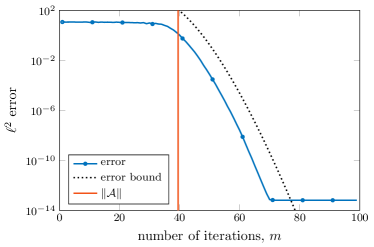
Figure 4.1: The Lanczos approximation to the matrix exponential for a random skew-Hermitian matrix $\mathcal{A}$ starts converging rapidly after $m\geq\left\|\mathcal{A}\right\|$.

In particular, it has been well documented that the side condition $m\geq\left\|\mathcal{A}\right\|$ is not an artificial imposition. In practice, Lanczos approximation of the exponential does not display superlinear convergence till the number of iterations have exceeded the spectral radius of the matrix $\mathcal{A}$ (see fig. 4.1).

5 Implementation

5.1 Approximation of integrals

Depending on $e$, analytic expressions for the integrals $\mbox{\boldmath$r$\unboldmath},\mbox{\boldmath$s$\unboldmath},\mbox{\boldmath$q$\unboldmath},\mbox{\boldmath$p$\unboldmath}$ and $c$ appearing in eq. 3.21, might be available. In the absence of analytic expressions, various quadrature methods can be utilised. For instance, if the quadrature weights and knots over $[0,h]$ are given by $w_{1},\ldots,w_{k}$ and $\zeta_{1},\ldots,\zeta_{k}$, respectively, we can approximate

$$\int_{0}^{h}\!f(h,\zeta)\mbox{\boldmath$e$\unboldmath}(t+\zeta)\,\mathrm{d}\zeta\approx\sum_{j=1}^{k}w_{j}f(h,\zeta_{j})\mbox{\boldmath$e$\unboldmath}(t+\zeta_{j}),$$ (5.1)

as usual. The nested integral in $c$, eq. 3.12, can be approximated as

$$\int_{0}^{h}\!\zeta\mbox{\boldmath$e$\unboldmath}(t+\zeta)^{\top}\int_{0}^{\zeta}\!\mbox{\boldmath$e$\unboldmath}(t+\xi)\,\mathrm{d}\xi\,\mathrm{d}\zeta\approx\sum_{i=1}^{k}\sum_{j=1}^{k}\widetilde{w}_{ij}\zeta_{i}\mbox{\boldmath$e$\unboldmath}(t+\zeta_{i})^{\top}\mbox{\boldmath$e$\unboldmath}(t+\zeta_{j}),$$ (5.2)

where the weights,

$$\widetilde{w}_{ij}=\int_{0}^{h}\!\ell_{i}(t+\zeta)\int_{0}^{\zeta}\!\ell_{j}(t+\xi)\,\mathrm{d}\xi\,\mathrm{d}\zeta,$$

are found by substituting the Lagrange interpolating polynomial for $e$,

$$\sum_{j=1}^{k}\ell_{j}(t+\zeta)\mbox{\boldmath$e$\unboldmath}(t+\zeta_{j}),\quad\ell_{j}(t+\zeta_{i})=\delta_{ij},$$

in the integral. For order six accuracy, for instance, Gauss–Legendre quadrature with three knots suffice for non-oscillatory potentials. In this case,

$$\mbox{\boldmath$w$\unboldmath}={\textstyle\frac{h}{18}}(5,8,5),\quad\mbox{\boldmath$\zeta$\unboldmath}={\textstyle\frac{h}{2}}\left(1-\sqrt{3/5},\ 1,\ 1+\sqrt{3/5}\right),$$

and

$$\widetilde{\mbox{\boldmath$w$\unboldmath}}=\frac{h^{2}}{648}\left(\begin{array}[]{ccc}25&40-12\sqrt{15}&25-6\sqrt{15}\\ 40+12\sqrt{15}&64&40-12\sqrt{15}\\ 25+6\sqrt{15}&40+12\sqrt{15}&25\\ \end{array}\right).$$

5.2 Computation of exponentials

The evaluation of exponentials of the modified kinetic and potential terms, $T_{k}$ and $W_{k}$, should be no more costly than the exponentiation of the Laplacian and the potential that are routinely employed in a sixth-order splitting scheme for time-independent potentials.

In eq. S2 and eq. S3, $C_{3}=C_{2}$ shares the structure of $T_{k}$s, and in eq. S3 $L_{3}$ has the same structure as $W_{k}$s. Consequently, the computation of their exponentials is not exceptionally problematic either. The commutator term in eq. S1, $C_{1}$, however, requires a different strategy and is exponentiated via Lanczos iterations.

5.2.1 Exponentiating the modified potential terms – $W_{k}$s and $L_{3}$

Under spectral collocation on an equispaced grid, the term $W_{1}$ in eq. S1 discretises to a diagonal matrix,

$$W_{1}\leadsto\mathcal{D}_{W_{1}}=\mathcal{D}_{-{\mathrm{i}}h\widetilde{V}+{\mathrm{i}}\varepsilon^{-1}\mbox{\boldmath$q$\unboldmath}^{\top}(\nabla V_{0})+c}\ ,$$

where $\leadsto$ denotes discretisation and $\mathcal{D}_{f}$ is a diagonal matrix with the values of $f$ on the grid points along its diagonal. The exponential of this is evaluated directly in a pointwise fashion,

$$\exp(\mathcal{D}_{f})=\mathcal{D}_{\exp(f)}.$$

The same holds true for the $W_{k}$s in eq. S2 and eq. S3, $L_{3}$ in eq. S3 and for exponentials of the form $\exp(bW+cU)$ in the splitting eq. OMF76.

5.2.2 Exponentiating the modified kinetic terms – $T_{k}$s and $C_{2}$

For the modified kinetic terms, we note that differentiation matrices are circulant and are diagonalised via Fourier transforms,

$$\partial_{x}^{k}\leadsto\mbox{\boldmath$D$\unboldmath}_{k,x}=\mathcal{F}_{x}^{-1}\mathcal{D}_{c_{k,x}}\mathcal{F}_{x},$$

where $\mathcal{F}_{x}$ is the Fourier transform in $x$ direction, $\mathcal{F}^{-1}_{x}$ is the inverse Fourier transform, $\mathcal{D}_{c_{k,x}}$ is a diagonal matrix and the values along its diagonal, $c_{k,x}$, comprise the symbol of the $k$th differentiation matrix, $\mbox{\boldmath$D$\unboldmath}_{k,x}$.

In two dimensions, for instance, the exponential of the Laplacian term, ${\mathrm{i}}h\varepsilon\Delta$, is routinely computed in exponential splitting schemes for Schrödinger equation with time-independent potentials as

$${\mathrm{e}}^{{\mathrm{i}}h\varepsilon\Delta}v\leadsto\mathcal{F}_{x}^{-1}\mathcal{D}_{\exp({\mathrm{i}}h\varepsilon c_{2,x})}\mathcal{F}_{x}\mathcal{F}_{y}^{-1}\mathcal{D}_{\exp({\mathrm{i}}h\varepsilon c_{2,y})}\mathcal{F}_{y}\mbox{\boldmath$v$\unboldmath},$$

using four Fast Fourier Transforms (FFTs).

Note that $\mathcal{F}_{y}\mbox{\boldmath$v$\unboldmath}$ is implemented in Matlab as fft(v,[],2) for $v$ discretised over an ndgrid domain, and $\mathcal{D}_{\mbox{\boldmath$a$\unboldmath}}\mbox{\boldmath$v$\unboldmath}$ is simply implemented as a.*v. Here $c_{2,x}$ and $c_{2,y}$ are the symbols of the differentiation matrices corresponding to $\partial_{x}^{2}$ and $\partial_{y}^{2}$, respectively. For instance, using a Fourier spectral method on an $[-L,L]^{2}$ box, where $\partial_{y}^{2}{\mathrm{e}}^{{\mathrm{i}}\pi(jx+ky)/L}=(-\pi^{2}k^{2}/L^{2}){\mathrm{e}}^{{\mathrm{i}}\pi(jx+ky)/L}$, we choose $(c_{2,y})_{j,k}=-\pi^{2}k^{2}/L^{2}$.

Using the same technique, we can compute the exponential of $T_{1}$ in eq. S1,

$${\mathrm{e}}^{{\mathrm{i}}h\varepsilon\Delta-\frac{1}{2}\mbox{\boldmath$s$\unboldmath}(t,h)^{\top}\nabla}v ={\mathrm{e}}^{{\mathrm{i}}h\varepsilon\partial_{x}^{2}-\frac{1}{2}s_{x}\partial_{x}}{\mathrm{e}}^{{\mathrm{i}}h\varepsilon\partial_{y}^{2}-\frac{1}{2}s_{y}\partial_{y}}v$$

$$\leadsto\mathcal{F}_{x}^{-1}\mathcal{D}_{\exp({\mathrm{i}}h\varepsilon c_{2,x}-\frac{1}{2}s_{x}c_{1,x})}\mathcal{F}_{x}\mathcal{F}_{y}^{-1}\mathcal{D}_{\exp({\mathrm{i}}h\varepsilon c_{2,x}-\frac{1}{2}s_{y}c_{1,x})}\mathcal{F}_{y}\mbox{\boldmath$v$\unboldmath},$$

where $\mbox{\boldmath$s$\unboldmath}=(s_{x},s_{y})$, without any additional FFTs. The same observations apply to $T_{k}$s and $C_{k}$s in eq. S2 and eq. S3.

5.2.3 Exponentiating the commutator term – $C_{1}$

Unlike $T_{k}$s and $W_{k}$s,

$$C_{1}=\left[\Delta,\mbox{\boldmath$p$\unboldmath}^{\top}(\nabla V_{0})\right],$$

which appears in eq. S1, does not possess a structure that allows for direct exponentiation. However, the spectral radius of $C_{1}$ upon discretisation,

$$C_{1}\leadsto\mbox{\boldmath$C$\unboldmath}_{1}=\left[\sum_{j=1}^{n}\mbox{\boldmath$D$\unboldmath}_{2,x_{j}}\ ,\ \mathcal{D}_{\mbox{\boldmath$p$\unboldmath}^{\top}(\nabla V_{0})}\right],$$

is very small since $\mbox{\boldmath$p$\unboldmath}={\cal O}\left(h^{5}\right)$. Since $\mbox{\boldmath$D$\unboldmath}_{k,x}$ scales as ${\cal O}\left((\Delta x)^{-k}\right)$,

$$\rho(\mbox{\boldmath$C$\unboldmath}_{1})=\left\|\mbox{\boldmath$C$\unboldmath}_{1}\right\|_{2}={\cal O}\left(h^{5}(\Delta x)^{-2}\right)\left\|\nabla V_{0}\right\|,$$

assuming that we use the same spatial resolution in all directions.

We can improve upon the estimate of the spectral radius further [22, 4], whereby we find $\rho(\mbox{\boldmath$C$\unboldmath}_{1})={\cal O}\left(h^{5}(\Delta x)^{-1}\right)\max_{i,j\in\{1,\ldots,n\}}\left\|\partial_{x_{i}}\partial_{x_{j}}V_{0}\right\|$. This improvement is notable in the semiclassical regime where a spatial resolution of $\Delta x={\cal O}\left(\varepsilon\right)$ is necessitated by the highly oscillatory solution.

This observation makes Lanczos iterations a very appealing candidate for the exponentiation of $\mbox{\boldmath$C$\unboldmath}_{1}$. As noted in section 4.4.4, these methods feature a superlinear accuracy once the number of Lanczos iterations has exceeded the spectral radius of the exponent. In practice, in the case of $\mbox{\boldmath$C$\unboldmath}_{1}$, we find ourselves in the regime of superlinear accuracy of Lanczos iterations almost immediately and even a single Lanczos iteration seems to be giving us very good results.

Each Lanczos iteration involves the computation of matrix-vector product of the form $\mbox{\boldmath$C$\unboldmath}_{1}\mbox{\boldmath$v$\unboldmath}$, which can be computed as

$$\mbox{\boldmath$C$\unboldmath}_{1}\mbox{\boldmath$v$\unboldmath} = \sum_{j=1}^{n}\mathcal{F}_{x_{j}}^{-1}\mathcal{D}_{c_{2,x_{j}}}\mathcal{F}_{x_{j}}\mathcal{D}_{\mbox{\boldmath$p$\unboldmath}^{\top}(\nabla V_{0})}\mbox{\boldmath$v$\unboldmath}-\mathcal{D}_{\mbox{\boldmath$p$\unboldmath}^{\top}(\nabla V_{0})}\sum_{j=1}^{n}\mathcal{F}_{x_{j}}^{-1}\mathcal{D}_{c_{2,x_{j}}}\mathcal{F}_{x_{j}}\mbox{\boldmath$v$\unboldmath}$$

via $4n$ FFTs. Since directions are independent, these can be parallelized. Alternatively, one may use four n-dimensional FFTs (such as Matlab’s fftn).

6 Numerical examples

In this section we provide detailed numerical experiments for two one-dimensional numerical examples considered by Iserles et al. [21] for which accurate reference solutions have been obtained by brute force (using extremely fine time steps and spatial grids).The first of these examples is in the regime, $\varepsilon_{1}=1$, and the second in the semiclassical regime of $\varepsilon_{2}=10^{-2}$. In both cases, we impose periodic boundaries on the spatial domains and resort to spectral collocation for discretisation.

In principle, the procedure extends in a straightforward way to higher dimensions via tensorisation of the periodic grids and we demonstrate the applicability of the approach using two and three-dimensional examples under $\varepsilon_{3}=\varepsilon_{4}=10^{-2}$. Lastly, we consider a Coloumb potential example from Schaeffer et al. [32] under $\varepsilon_{5}=1$.

In the first two examples, the initial conditions $u_{0,1}$ and $u_{0,2}$ are Gaussian wavepackets,

$$u_{0,k}(x)=(\delta_{k}\pi)^{-d/4}\exp\left((-(x-x_{0})^{2})/(2\delta_{k})\right),\quad x_{0}=-2.5,\ k=1,2,$$

with $d=1$ (for the one dimensional problems), $\delta_{1}=0.2$ and $\delta_{2}=10^{-2}$ in the respective cases. These wavepackets are sitting in the left well of the double well potentials,

$$V_{1}(x)=x^{4}-15x^{2}\quad\mathrm{and}\quad V_{2}(x)={\textstyle\frac{1}{5}}x^{4}-2x^{2},$$

respectively, which act as the choice of $V_{0}$ in the two examples. The time profile of the laser used here is

$$e_{1}(t)=\begin{cases}\sin(25\pi t)&\quad t\in[{\textstyle\frac{3}{5}}n,{\textstyle\frac{3}{5}}n+{\textstyle\frac{1}{25}}],\quad n\geq 1,\\ \sin(5\pi t)&\quad t\in({\textstyle\frac{3}{5}}n+{\textstyle\frac{1}{25}},{\textstyle\frac{3}{5}}n+{\textstyle\frac{6}{25}}],\quad n\geq 1,\end{cases}$$

and

$$e_{2}(t)=10\exp(-10(t-1)^{2})\sin((500(t-1)^{4}+10)),$$

respectively. The former is a sequence of asymmetric sine lobes while the latter is a highly oscillatory chirped pulse (fig. 6.2 (left)). Such laser profiles are used routinely in laser control [3]. Even more oscillatory electric fields often result from optimal control algorithms [25, 13].

The spatial domain is $[-10,10]$ and $[-5,5]$ in the two examples, respectively, while the temporal domain is $[0,4]$ and $[0,\frac{5}{2}]$, respectively.

In the third and fourth examples, we consider the Gaussian wavepackets

$$u_{0,k}(x)=(\delta_{k}\pi)^{-d/4}\exp\left(-\left\|\mbox{\boldmath$x$\unboldmath}\right\|^{2}/(2\delta_{k})\right),\quad k=3,4,$$

with $d=2$ for a two-dimensional example (example 3) and $d=3$ for a three-dimensional example (example 4). We use $\delta_{3}=\delta_{4}=10^{-3}$ and $\varepsilon_{3}=\varepsilon_{4}=10^{-2}$ in both cases. These wavepackets are sitting in the central wells of the potentials

$$V_{3}(\mbox{\boldmath$x$\unboldmath})=2500\prod_{j=1}^{4}\left\|\mbox{\boldmath$x$\unboldmath}-\mbox{\boldmath$c$\unboldmath}_{j}\right\|^{2},\qquad V_{4}(\mbox{\boldmath$x$\unboldmath})=40\prod_{j=1}^{5}\left\|\mbox{\boldmath$x$\unboldmath}-\mbox{\boldmath$c$\unboldmath}_{j}\right\|^{2},$$

which are degree eight and degree ten polynomials in two and three dimensions, respectively, and where the wells are defined by the centres,

$$\left(\mbox{\boldmath$c$\unboldmath}_{1},\ldots,\mbox{\boldmath$c$\unboldmath}_{4}\right)=\left(\begin{array}[]{ccccc}-0.5&-0.5&1/\sqrt{2}&0\\ -0.5&0.5&0&0\\ \end{array}\right),\quad\left(\mbox{\boldmath$c$\unboldmath}_{1},\ldots,\mbox{\boldmath$c$\unboldmath}_{5}\right)=\left(\begin{array}[]{ccccc}-0.5&-0.5&0.75&0&0\\ -0.5&0.5&0&0&0\\ -0.5&-0.5&-0.5&0&0.75\\ \end{array}\right),$$

in the two cases, respectively. The spatial domain used is $[-1,1]^{d}$ and the temporal domain is $[0,2]$. In the two dimensional case (fig. 6.3) we consider the influence under a laser in the $x$ direction (fig. 6.4 (left)), while in the three dimensional case we consider lasers in two different directions of polarisation (fig. 6.4 (centre) and (right)),

$$\mbox{\boldmath$e$\unboldmath}_{3}(t)=\frac{e_{2}(t)}{5}(1,0)^{\top},\qquad\mbox{\boldmath$e$\unboldmath}_{4,1}(t)=\frac{e_{2}(t)}{5}(0,0,1)^{\top},\quad\mbox{\boldmath$e$\unboldmath}_{4,2}(t)=\frac{e_{2}(t)}{5\sqrt{2}}(-1,0,1)^{\top}.$$

Lastly, we consider the one-dimensional (soft) Coloumb potential example from Schaeffer et al. [32] as our fifth example (fig. 6.2 (centre) and (right)), where $V_{5}(x)=2\left(1-{\textstyle\frac{1}{\sqrt{x^{2}+1}}}\right)$. We take the (numerically determined) fifth eigenfunction of this potential as the initial condition, $u_{0,5}$, and consider its evolution under the influence of the laser profile

$$e_{5}(t)=-0.01\ \mathrm{sech}\left(\frac{t-250}{85}\right)\cos(0.12\,(t-250)),$$

over a temporal domain $[0,500]$ and spatial domain $[-240,240]$. The temporal domain is halved and the potential scaled up by a factor of two to account for the fact that under our scaling $\Delta$ appears without a factor of $1/2$ in eq. 1.1.

The effective time-dependent potentials in our examples are

$$V_{e,k}(\mbox{\boldmath$x$\unboldmath},t)=V_{k}(\mbox{\boldmath$x$\unboldmath})+\mbox{\boldmath$e$\unboldmath}_{k}(t)^{\top}\mbox{\boldmath$x$\unboldmath},\quad k=1,2,3,4,5,$$

with an additional index being used in the case of $k=4$ to distinguish the use of $\mbox{\boldmath$e$\unboldmath}_{4,1}$ or $\mbox{\boldmath$e$\unboldmath}_{4,2}$. Under the influence of these potentials, the initial conditions evolve to $u_{e,k}(T)$ at $t=T$. The probability of being within a radius of $0.2$ from the centres $\mbox{\boldmath$c$\unboldmath}_{j}$ in the two and three-dimensional examples under the influence of these lasers is shown in fig. 6.4.

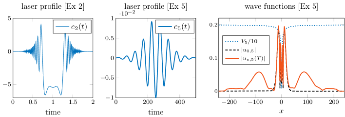
Figure 6.2: [Ex 2, 5] Laser profiles $e_{2}$ (left) and $e_{5}$ (centre). The fifth eigenfunction of the soft Coloumb potential $V_{5}$ evolves to $u_{e,5}(T)$ at $t=T$ under the influence of $e_{5}$ (right).

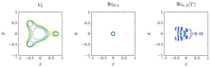
Figure 6.3: [Ex 3] The potential $V_{3}$ in two dimensions shown with contour lines (left); initial condition $u_{0,3}$ (centre) evolves to to $u_{e,3}(T)$ (right) under the influence of $e_{3}(t)={\textstyle\frac{1}{5}}e_{2}(t)(1,0)^{\top}$. Contour lines for the potential range from $0$ to $2$, while those for (real part of the) wavefunctions range from $0.25$ to $4$. The levels are separated by $0.25$ in all cases. Here, the semiclassical parameter is $\varepsilon_{3}=1/100$.

Figure 6.4: [Well Occupation] Probability of particle being in a radius $0.2$ from the centres $\mbox{\boldmath$c$\unboldmath}_{j}$ in two dimensions under the influence of $\mbox{\boldmath$e$\unboldmath}_{3}(t)$ (left) and in three dimensions under the influence of $\mbox{\boldmath$e$\unboldmath}_{4,1}(t)$ (centre) and $\mbox{\boldmath$e$\unboldmath}_{4,2}(t)$ (right).

Methods. In figs. 6.6 and 6.5 we display the comparisons of accuracy and efficiencies of several methods. The naming of methods is straightforward – the combination of the $n$-th proposed scheme with the $k$-th splitting (the splitting described by the coefficients in eq ($k$)) of Omelyan et al. [28] is labeled S$n$OMF$k$. For instance, the combination of eq. S2 with eq. OMF76, which describes a concrete scheme will be called S2OMF76, while the combination of eq. S3 with eq. OMF85 will be called S3OMF85. In the case of eq. S1, we add the postfix L$m$ to denote the number of Lanczos iterations used for $C_{1}$.

These methods are also compared against OMF$k$ (without a prefix of S$n$), which denote the time-ordered exponential splittings given by the coefficients in eq ($k$) of Omelyan et al. [28] that handle a time-dependent potential by advancing time along with the application of the Laplacian [14]. These are an alternative to the proposed approach that were mentioned in the introduction.

Commutator-free Lanczos based methods [2] are not compared against the proposed schemes since their relative ineffectiveness in the context of eq. 1.1 has already been studied [21].

In the first example $\varepsilon_{1}=1$, we use $M_{1}=150$ spatial grid points while for second example, which features highly oscillatory behaviour in the solution due to the small semiclassical parameter $\varepsilon_{2}=10^{-2}$, we use $M_{2}=1000$ spatial grid points (which, nevertheless, proves inadequate to achieve accuracies higher than $10^{-6}$). In the third and fourth we use $M=150$ points in each direction to keep computations manageable. This low spatial resolution limits the accuracy that can be achieved. In the final example, we use $M=768$ points for the Coloumb potential.

Absorbing boundary. We use an absorbing boundary of width $40$ using the procedure described in section 4.2 of Schaeffer et al. [32]. In particular, we need to compute the potential $V_{mod}$ which is a version of $V_{e,5}(x,t)$ that smoothly becomes flat in the absorbing boundary region (eq. (103) of Schaeffer et al. [32]). In principle this needs to be computed at each $t$. The problem is more easily resolved by computing the flattened versions $V_{5,mod}$ and $x_{mod}$ for $V_{5}$ and $x$ once, after which the flattened version of $V_{e,5}(x,t)$ can readily be computed as $V_{5,mod}+e_{5}(t)x_{mod}$ for any $t$. This directly leads to a flattened version of $\tilde{V}$ required in eq. S3, to which we add the complex-valued absorbing potential from Schaeffer et al. [32] to complete the description.

Reference solution. In the first example the reference solution is obtained by using a sixth-order Magnus–Lanczos method [5], while in the second example the reference solution is obtained using a sixth-order commutator-free Lanczos based method [2]. In both cases we used $5000$ spatial grid points and $10^{6}$ time steps. For the third and fourth examples, we generate a reference solution with $150$ grid points in each direction due to computational complexity, using Strang splitting with $2\times 10^{6}$ time steps for the third example and OMF80 with $10^{4}$ time steps for the fourth example. The reference solution for the fifth example is generated using OMF85 with $2\times 10^{5}$ time steps.

Quadrature points. In the first example, the integrals in our schemes are discretised via three Gauss–Legendre knots, while in the second example eleven Gauss–Legendre knots are used in order to adequately resolve the highly oscillatory potential. In contrast, the method OMF$k$ effectively use a fixed number of knots, dictated by the number of exponentials of the Laplacian. For instance, eq. OMF76 and OMF80 use five knots while OMF71 uses six knots.

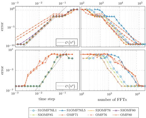
Figure 6.5: [Ex 1 (top), Ex 2 (bottom)] accuracy (left); efficiency (right).

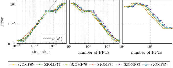
Figure 6.6: Accuracy (left) and efficiency for Ex 1 (centre); efficiency for Ex 2 (right).

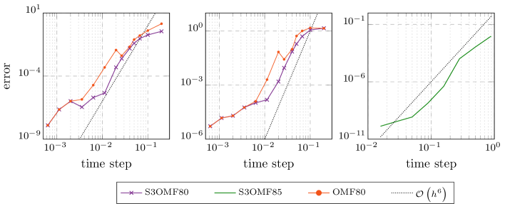
Figure 6.7: Accuracy for Ex 3 (left), Ex 4 under $\mbox{\boldmath$e$\unboldmath}_{4,1}(t)$ (centre) and Ex 5 (right).

7 Conclusions

We have presented three different strategies for easily extending existing sixth-order schemes for the Schrödinger equation with time-independent potentials to the case of laser potentials under the dipole approximation. The overall schemes require, at most, one additional exponential, which leads to a very marginal increase in cost.

Keeping the integrals $\mbox{\boldmath$r$\unboldmath},\mbox{\boldmath$s$\unboldmath},\mbox{\boldmath$q$\unboldmath},\mbox{\boldmath$p$\unboldmath}$ and $c$ intact in our schemes allows us flexibility in deciding a quadrature strategy at the very end. The advantage over the time-ordered exponential splittings OMF71, OMF76 and OMF80, which sample the potential at fixed time knots, is evident from the numerical results for the second example (fig. 6.5 (bottom row)), where a highly oscillatory laser is involved. Where a weaker field is involved (such as Examples 3 and 4 where $\left\|\mbox{\boldmath$e$\unboldmath}_{3}(t)\right\|=\left\|\mbox{\boldmath$e$\unboldmath}_{4,1}(t)\right\|=\left\|\mbox{\boldmath$e$\unboldmath}_{4,2}(t)\right\|=\left\|\mbox{\boldmath$e$\unboldmath}_{2}(t)\right\|/5$) and the solution is less oscillatory, the advantage may be less pronounced (fig. 6.7 (left) and (centre)).

Moreover, as mentioned in the introduction, preserving the integrals till the end allows us to use other quadrature methods which can be particularly helpful when the laser potential is only known at specific points (such as in control applications).

The proposed methods are also effective when the potential is not highly oscillatory and can be sampled arbitrarily. As seen by numerical results for the first example (fig. 6.5 (top row)), the proposed schemes end up being very effective (nearly as accurate as the sixth-order methods) even when combined with OMF71 and OMF80, which are fourth-order schemes with low error constants. This is in contrast to the direct use of OMF71 and OMF80 as time-ordered exponential splittings. A comparison of some fourth and sixth-order splittings from Omelyan et al. [28] for the central exponent is presented in fig. 6.6.

Where the gradient of the potential, $\nabla V_{0}$, is available, we recommend using eq. S2 in conjunction with compact splittings such as eq. OMF76. Where $\nabla V_{0}$ needs to be avoided, we recommend using eq. S3 in conjunction with classical splittings such as eq. OMF85 or OMF80. The effectiveness of such a gradient free scheme, S3OMF85, is demonstrated for the soft Coloumb potential of Example 5 in fig. 6.7 (right).

We remind the reader that the splitting schemes of Omelyan et al. [28] are among a myriad possible ways of approximating the innermost exponential, $\exp(T+W)$, in eq. 4.1. As mentioned in section 4.4, for instance, alternative methods such as Lanczos approximation [29] and Chebychev approximation [35] can also be employed for this purpose. In contrast to a direct application of these techniques for exponentiating the Magnus expansion, the application to $\exp(T+W)$ would benefit from lower costs of matrix-vector products due to a commutator-free exponent. The primary focus of this manuscript, however, is to present a few general strategies (the splittings eqs. S1, S2 and S3) for extending existing schemes to the case of laser potentials, and the potential merits and limitations of following this approach in the context of various existing schemes have not been fully explored.

While the numerical examples demonstrate the effectiveness of the schemes for laser potentials in one, two and three dimensions (in Cartesian coordinates), there are a range of issues and possible avenues of future research that our work raises:

1. High dimensions. For dimensions higher than three, tensorisation is not a viable strategy. Among the various approaches for truly high-dimensional problems, the extension of the proposed schemes to the case of Hagedorn wavepackets [16] is worth exploring since the additional terms in our schemes are at most quadratic in the momentum and position operators, $-{\mathrm{i}}\nabla$ and $x$.

2. Non-Cartesian coordinates. While applicability of this approach to vibrational coordinates is unlikely, an approach for spherical coordinates using a mix of Fast Spherical Harmonic Transforms and Fast Fourier Transforms is being explored.

3. Matrix-valued potentials. In the coherent control of a two-level atom [33], the potential becomes matrix-valued. The change in the algebraic nature of the problem necessitates the development of specialised splittings for this case.

Appendix A Scalar phase factors

A.1 Simplification of $c_{3,1}$

For the simplification of the integrals in $c_{3,1}$, we define

$$I_{1} = \int_{0}^{h}\!\zeta\mbox{\boldmath$e$\unboldmath}(t+\zeta)^{\top}\int_{0}^{\zeta}\!\mbox{\boldmath$e$\unboldmath}(t+\xi)\,\mathrm{d}\xi\,\mathrm{d}\zeta,$$

$$I_{2} = \int_{0}^{h}\!\left(\int_{0}^{\zeta}\!\mbox{\boldmath$e$\unboldmath}(t+\xi)\,\mathrm{d}\xi\right)^{2}\,\mathrm{d}\zeta,$$

$$I_{3} = \int_{0}^{h}\!\mbox{\boldmath$e$\unboldmath}(t+\zeta)^{\top}\int_{0}^{\zeta}\!\xi\mbox{\boldmath$e$\unboldmath}(t+\xi)\,\mathrm{d}\xi\,\mathrm{d}\zeta,$$

and derive the following identities via integration by parts,

$$I_{2}=-I_{1}+I_{3}+\left(\int_{0}^{h}\!\mbox{\boldmath$e$\unboldmath}(t+\zeta)\,\mathrm{d}\zeta\right)^{\top}\left(\int_{0}^{h}\!(h-\zeta)\mbox{\boldmath$e$\unboldmath}(t+\zeta)\,\mathrm{d}\zeta\right),$$

and

$$I_{3}=-I_{1}+\left(\int_{0}^{h}\!\mbox{\boldmath$e$\unboldmath}(t+\zeta)\,\mathrm{d}\zeta\right)^{\top}\left(\int_{0}^{h}\!\zeta\mbox{\boldmath$e$\unboldmath}(t+\zeta)\,\mathrm{d}\zeta\right),$$

so that $I_{2}=-2I_{1}+h\left(\int_{0}^{h}\!\mbox{\boldmath$e$\unboldmath}(t+\zeta)\,\mathrm{d}\zeta\right)^{2}$, where $\mbox{\boldmath$a$\unboldmath}^{2}=\mbox{\boldmath$a$\unboldmath}^{\top}\mbox{\boldmath$a$\unboldmath}$. Putting these together,

$$c_{3,1} ={\textstyle\frac{1}{6}}{\mathrm{i}}\varepsilon^{-1}\int_{0}^{h}\!\int_{0}^{\zeta}\!(\mbox{\boldmath$e$\unboldmath}(t+\zeta)-\mbox{\boldmath$e$\unboldmath}(t+\xi))^{\top}\int_{0}^{\zeta}\!\mbox{\boldmath$e$\unboldmath}(t+\chi)\,\mathrm{d}\chi\,\mathrm{d}\xi\,\mathrm{d}\zeta$$

$$={\textstyle\frac{1}{6}}{\mathrm{i}}\varepsilon^{-1}(I_{1}-I_{2})={\mathrm{i}}\varepsilon^{-1}\left({\textstyle\frac{1}{2}}I_{1}-{\textstyle\frac{1}{6}}h\left(\int_{0}^{h}\!\mbox{\boldmath$e$\unboldmath}(t+\zeta)\,\mathrm{d}\zeta\right)^{2}\right).$$ (A.1)

A.2 Simplification of $c_{3,2}$

For the simplification of $c_{3,2}$, we simplify

$$\int_{0}^{h}\!\mbox{\boldmath$e$\unboldmath}(t+\zeta)^{\top}\int_{0}^{\zeta}\!\int_{0}^{\xi}\!\mbox{\boldmath$e$\unboldmath}(t+\chi)\,\mathrm{d}\chi\,\mathrm{d}\xi\,\mathrm{d}\zeta-\int_{0}^{h}\!\mbox{\boldmath$e$\unboldmath}(t+\zeta)^{\top}\int_{0}^{\zeta}\!\int_{0}^{\xi}\!\mbox{\boldmath$e$\unboldmath}(t+\xi)\,\mathrm{d}\chi\,\mathrm{d}\xi\,\mathrm{d}\zeta$$

$$\qquad=\int_{0}^{h}\!\mbox{\boldmath$e$\unboldmath}(t+\zeta)^{\top}\int_{0}^{\zeta}\!(\zeta-\xi)\mbox{\boldmath$e$\unboldmath}(t+\xi)\,\mathrm{d}\xi\,\mathrm{d}\zeta-\int_{0}^{h}\!\mbox{\boldmath$e$\unboldmath}(t+\zeta)^{\top}\int_{0}^{\zeta}\!\xi\mbox{\boldmath$e$\unboldmath}(t+\xi)\,\mathrm{d}\xi\,\mathrm{d}\zeta$$

$$\qquad=I_{1}-2I_{3}=3I_{1}-2\left(\int_{0}^{h}\!\mbox{\boldmath$e$\unboldmath}(t+\zeta)\,\mathrm{d}\zeta\right)^{\top}\left(\int_{0}^{h}\!\zeta\mbox{\boldmath$e$\unboldmath}(t+\zeta)\,\mathrm{d}\zeta\right).$$

using eq. 3.4 under $n=0$. Consequently,

$$c_{3,2} ={\textstyle\frac{1}{2}}{\mathrm{i}}\varepsilon^{-1}\int_{0}^{h}\!\mbox{\boldmath$e$\unboldmath}(t+\zeta)^{\top}\int_{0}^{\zeta}\!\int_{0}^{\xi}\!\mbox{\boldmath$e$\unboldmath}(t+\chi)-\mbox{\boldmath$e$\unboldmath}(t+\xi)\,\mathrm{d}\chi\,\mathrm{d}\xi\,\mathrm{d}\zeta$$

$$={\mathrm{i}}\varepsilon^{-1}\left({\textstyle\frac{3}{2}}I_{1}-\left(\int_{0}^{h}\!\mbox{\boldmath$e$\unboldmath}(t+\zeta)\,\mathrm{d}\zeta\right)^{\top}\left(\int_{0}^{h}\!\zeta\mbox{\boldmath$e$\unboldmath}(t+\zeta)\,\mathrm{d}\zeta\right)\right).$$ (A.2)

Putting these together, $c(t,h)=c_{3,1}+c_{3,2}$,

$$c(t,h)={\mathrm{i}}\varepsilon^{-1}\left(2I_{1}-\left(\int_{0}^{h}\!\mbox{\boldmath$e$\unboldmath}(t+\zeta)\,\mathrm{d}\zeta\right)^{\top}\left(\int_{0}^{h}\!\zeta\mbox{\boldmath$e$\unboldmath}(t+\zeta)\,\mathrm{d}\zeta\right)-{\textstyle\frac{1}{6}}h\left(\int_{0}^{h}\!\mbox{\boldmath$e$\unboldmath}(t+\zeta)\,\mathrm{d}\zeta\right)^{2}\right).$$ (3.12)

References

• [1] H. Agueny, M. Chovancova, J. P. Hansen, and L. Kocbach. Scaling properties of field ionization of Rydberg atoms in single-cycle THz pulses: 1d considerations. J. Phys. B: At. Mol. Opt. Phys., 49:245002, 2016.
• [2] A. Alvermann and H. Fehske. High-order commutator-free exponential time-propagation of driven quantum systems. J. Comput. Phys., 230(15):5930–5956, 2011.
• [3] B. Amstrup, J. D. Doll, R. A. Sauerbrey, G. Szabó, and A. Lorincz. Optimal control of quantum systems by chirped pulses. Phys. Rev. A, 48(5):3830–3836, Nov 1993.
• [4] Philipp Bader, Arieh Iserles, Karolina Kropielnicka, and Pranav Singh. Effective approximation for the semiclassical Schrödinger equation. Found. Comput. Math., 14:689–720, 2014.
• [5] Philipp Bader, Arieh Iserles, Karolina Kropielnicka, and Pranav Singh. Efficient methods for linear Schrödinger equation in the semiclassical regime with time-dependent potential. Proc. Royal Soc. A., 472(2193):20150733, 18, 2016.
• [6] André D. Bandrauk and Huizhong Lu. Exponential propagators (integrators) for the time-dependent Schrödinger equation. J. Theor. Comput. Chem., 12(06):1340001, sep 2013.
• [7] S. Blanes, F. Casas, and A. Murua. Symplectic splitting operator methods tailored for the time-dependent Schrödinger equation. J. Chem. Phys., 124:105–234, 2006.
• [8] S. Blanes, F. Casas, and A. Murua. Splitting and composition methods in the numerical integration of differential equations. Bol. Soc. Esp. Mat. Apl., 45:89–145, 2008.
• [9] S. Blanes, F. Casas, and J. Ros. Improved high order integrators based on the Magnus expansion. BIT, 40(3):434–450, 2000.
• [10] S. Blanes and P. C. Moan. Practical symplectic partitioned Runge-Kutta and Runge-Kutta-Nyström methods. J. Comput. Appl. Math., 142(2):313–330, 2002.
• [11] Sergio Blanes, Fernando Casas, and Ander Murua. Symplectic time-average propagators for the Schrödinger equation with a time-dependent Hamiltonian. J. Chem. Phys., 146(11):114109, 2017.
• [12] Sergio Blanes, Fernando Casas, and Mechthild Thalhammer. High-order commutator-free quasi-Magnus exponential integrators for non-autonomous linear evolution equations. Comput. Phys. Commun., 220:243 – 262, 2017.
• [13] L. H. Coudert. Optimal control of the orientation and alignment of an asymmetric-top molecule with terahertz and laser pulses. J. Chem. Phys., 148(9):094306, 2018.
• [14] G Goldstein and D Baye. Sixth-order factorization of the evolution operator for time-dependent potentials. Phys. Rev. E, 70(5):056703, nov 2004.
• [15] G. H. Golub and C. F. Van Loan. Matrix Computations. Johns Hopkins University Press, Baltimore, 3rd edition, 1996.
• [16] Vasile Gradinaru and George A. Hagedorn. Convergence of a semiclassical wavepacket based time-splitting for the Schrödinger equation. Numer. Math., 126(1):53–73, 2014.
• [17] M. Hochbruck and C. Lubich. On Krylov subspace approximations to the matrix exponential operator. SIAM J. Numer. Anal., 34:1911–1925, 1997.
• [18] A. Iserles, H. Z. Munthe-Kaas, S. P. Nørsett, and A. Zanna. Lie-group methods. Acta Numerica, 9:215–365, 2000.
• [19] A. Iserles and S. P. Nørsett. On the solution of linear differential equations in Lie groups. Phil. Trans. Royal Soc. A, 357:983–1020, 1999.
• [20] Arieh Iserles, Karolina Kropielnicka, and Pranav Singh. Magnus–Lanczos methods with simplified commutators for the Schrödinger equation with a time-dependent potential. SIAM J. on Numer. Anal., 56(3):1547–1569, 2018.
• [21] Arieh Iserles, Karolina Kropielnicka, and Pranav Singh. Compact schemes for laser–matter interaction in Schrödinger equation based on effective splittings of Magnus expansion. Comput. Phys. Commun., 234:195 – 201, 2019.
• [22] Arieh Iserles, Karolina Kropielnicka, and Pranav Singh. Solving Schrödinger equation in semiclassical regime with highly oscillatory time-dependent potentials. J. Comput. Phys., 376:564 – 584, 2019.
• [23] M. Klaiber, D. Dimitrovski, and J.S. Briggs. Magnus expansion for laser-matter interaction: application to generic few-cycle laser pulses. Phys. Rev. A, 79(4):3830–3836, April 2009.
• [24] R. I. McLachlan and G. R. W. Quispel. Splitting methods. Acta Numerica, 11:341–434, 2002.
• [25] H. Meyer, L. Wang, and V. May. Optimal control of multidimensional vibronic dynamics: algorithmic developments and applications to 4d-Pyrazine. In B. Lasorne and G. A. Worth, editors, Proceedings of the CCP6 workshop on Coherent Control of Molecules, pages 50–55. CCP6, July 2006.
• [26] Hans Munthe-Kaas and Brynjulf Owren. Computations in a free Lie algebra. Phil. Trans. Royal Soc. A, 357(1754):957–981, 1999.
• [27] Mamadou Ndong, Hillel Tal-Ezer, Ronnie Kosloff, and Christiane P. Koch. A Chebychev propagator with iterative time ordering for explicitly time-dependent Hamiltonians. J. Chem. Phys., 132(6):064105, 2010.
• [28] I.P. Omelyan, I.M. Mryglod, and R. Folk. Symplectic analytically integrable decomposition algorithms: classification, derivation, and application to molecular dynamics, quantum and celestial mechanics simulations. Comput. Phys. Commun., 151(3):272 – 314, 2003.
• [29] Tae Jun Park and J. C. Light. Unitary quantum time evolution by iterative Lanczos reduction. J. Chem. Phys., 85(10):5870–5876, 1986.
• [30] Uri Peskin, Ronnie Kosloff, and Nimrod Moiseyev. The solution of the time dependent Schrödinger equation by the (t,t’) method: The use of global polynomial propagators for time dependent Hamiltonians. J. Chem. Phys., 100(12):8849–8855, 1994.
• [31] J. M. Sanz-Serna and A. Portillo. Classical numerical integrators for wave‐packet dynamics. J. Chem. Phys., 104(6):2349–2355, 1996.
• [32] Ido Schaefer, Hillel Tal-Ezer, and Ronnie Kosloff. Semi-global approach for propagation of the time-dependent Schrödinger equation for time-dependent and nonlinear problems. J. Comput. Phys., 343:368–413, 2017.
• [33] M. Shapiro and P. Brumer. Principles of the Quantum Control of Molecular Processes. Wiley-Interscience, Hoboken, N.J., 2003.
• [34] Masuo Suzuki. General decomposition theory of ordered exponentials. Proc. Jpn. Acad., Ser. B, 69(7):161–166, 1993.
• [35] H. Tal Ezer and R. Kosloff. An accurate and efficient scheme for propagating the time dependent Schrödinger equation. J. Chem. Phys., 81:3967–3976, 1984.
• [36] Hillel Tal-Ezer, Ronnie Kosloff, and Charles Cerjan. Low-order polynomial approximation of propagators for the time-dependent Schrödinger equation. J. Comput. Phys., 100(1):179–187, 1992.
• [37] Jean Christophe Tremblay and Tucker Carrington Jr. Using preconditioned adaptive step size Runge–Kutta methods for solving the time-dependent Schrödinger equation. J. Chem. Phys., 121(23):11535–11541, 2004.