Large $N$ phase transition in $T\overline{T}$-deformed $2d$ Yang–Mills theory on the sphere

Abstract

We study the partition function of a $T\overline{T}$-deformed version of Yang–Mills theory on the two-sphere. We show that the Douglas–Kazakov phase transition persists for a range of values of the deformation parameter, and that the critical area is lowered. The transition is of third order and also induced by instantons, whose contributions we characterize.

1 Introduction

Low dimensional quantum field theories have been proved for decades to be a very valuable source of exact results, providing numerous insights into quantum theory as well as showing many direct relationships with statistical mechanical systems, strongly correlated systems and integrable systems, just to name a few. In recent years, a certain deformation of two-dimensional relativistic quantum field theories, based on the specific properties, described by Zamolodchikov in Zamolodchikov:2004ce , of the $T_{zz}T_{\bar{z}\bar{z}}-T_{z\bar{z}}^{2}$ operator, also known as $T\overline{T}$ operator and where $T_{zz}$ denotes the components of the stress tensor in complex coordinates, is attracting a considerable amount of interest.

The vacuum expectation of the operator has distinctive properties Zamolodchikov:2004ce and irrelevant deformations by this operator were studied in Smirnov:2016lqw ; Cavaglia:2016oda , showing that, after compactification of the theory on a Euclidean circle of radius $R$, a simple differential equation (a Burgers equation) governs how the energy spectrum at finite $R$ evolves according to a parameter $\tau$, which controls the strength of the deformation by the $T\overline{T}$ operator.

A large number of works involving this deformation have appeared already, including work showing that the deformation is equivalent to coupling the theory to flat space Jackiw–Teitelboim gravity such that at high energies is a gravitational theory with no local degrees of freedom Dubovsky:2017cnj ; Dubovsky:2018bmo and a number of other results (see for example Giveon:2017nie ; Giveon:2017myj ; Datta:2018thy ; Aharony:2018bad ; Cardy:2018sdv ; Conti:2018tca ), including also results for non-relativistic systems Cardy:2018jho .

We will not be using any of these developments specifically but, rather, will take on the last part of the recent work Conti:2018jho , where the $T\overline{T}$-deformation of two-dimensional Yang–Mills theory Cordes:1994fc is presented. We shall focus on the case of the sphere and see how two of the most salient features of the original theory still hold, but are modified by the deformation. Namely, the Douglas–Kazakov large $N$ phase transition of the theory and the proof that such phase transition is induced by (unstable) instantons.

The paper is organized as follows: we introduce below the basics of two-dimensional Yang–Mills theory and its $T\overline{T}$-deformation. In Section 2, we study the large $N$ behavior of the partition function, following Douglas:1993iia , and obtain a phase transition with a critical area modified by a factor, that we fully specify. We characterize both the weak-coupling and the strong-coupling phase, with the former still being described by a Wigner semicircle distribution for the eigenvalues, but with a nontrivial rescaling of the area parameter. Note that the existence of the weak-coupling phase is dependent on the value of the $\tau$ parameter. In particular, there are values of the deformation, given by $\tau\geq 12\pi^{2}/(12-\pi^{2})$, for which there is only the strong-coupling phase.

As happens in the undeformed case, the recursion involved in the strong-coupling phase is more complicated, but we characterize the nonperturbative solution near the critical point. The phase transition is found to be of third order, as in the undeformed case.

In Section 3, we explore what happens with the well-known and elegant explanation of the phase transition as triggered by instantons Gross:1994mr . For this, we use the corresponding matrix model description for the deformed theory and obtain that the same mechanism is at work, and moreover we are able to quantify the (stronger) effects of the instantonic contributions. Finally, we conclude with avenues for further work.

1.1 Two-dimensional Yang–Mills theory and its $T\overline{T}$-deformation

We review quantum Yang–Mills theory with gauge group $SU(N)$ on an oriented closed Riemann surface $\Sigma_{h}$ of genus $h$ and unit area form $\mathrm{d}\mu$ Cordes:1994fc . The action is

$$S_{\mathrm{YM}}=-\frac{1}{4g^{2}}\,\int_{\Sigma_{h}}\,\mathrm{d}\mu\leavevmode\nobreak\ \mathrm{Tr}\,F^{2}\ ,$$ (1.1)

where $g^{2}$ plays the role of the coupling constant, $F$ is the field strength of a matrix gauge connection, and $\mathrm{Tr}$ is the trace in the fundamental representation of $SU(N)$. Migdal discussed the lattice regularization of the gauge theory, which relies on a triangulation of the two-dimensional manifold $\Sigma_{h}$ with group matrices situated along the edges Migdal:1975zg . The path integral is then approximated by the finite-dimensional unitary matrix integral

$$\mathcal{Z}_{\mathrm{M}}=\int\,\prod_{\mathrm{edges}\leavevmode\nobreak\ \ell}\,\mathrm{d}U_{\ell}\leavevmode\nobreak\ \prod\limits_{\mathrm{plaquettes}\leavevmode\nobreak\ P}\,Z_{P}\left[U_{P}\right]\ ,$$ (1.2)

where $\mathrm{d}U_{\ell}$ denotes Haar measure on $SU(N)$ and the holonomy $U_{P}=\prod\nolimits_{\ell\in P}\,U_{\ell}$ is the ordered product of group matrices along the links of a given plaquette. The local factor $Z_{P}\left[U_{P}\right]$ is a suitable gauge invariant lattice weight that converges in the continuum limit to the Boltzmann weight for the Yang–Mills action (1.1). The use of the heat kernel lattice action for the lattice weight $Z_{P}\left[U_{P}\right]$, has very relevant features Menotti:1981ry and is the usual choice in two-dimensional Yang–Mills theory Cordes:1994fc . It leads to the group theory expansion of the partition function Migdal:1975zg ; Rusakov:1990rs

$$\mathcal{Z}_{\mathrm{M}}=\sum_{R}\,\left(\dim R\right)^{2-2h}\,\exp\big{(}-\frac{g^{2}A}{2}\,C_{2}(R)\big{)}\ ,$$ (1.3)

where the sum runs over all isomorphism classes $R$ of irreducible representations of the $SU(N)$ gauge group, $\dim R$ is the dimension of the representation $R$ and $C_{2}(R)$ is the quadratic Casimir invariant of $R$. The $g^{2}$ is the Yang–Mills coupling, and $A$ is a parameter which can be identified with the area of the surface. In the following, we shall focus on $U(N)$ gauge theory, instead of $SU(N)$, so we use the identification $U(N)=SU(N)\times U(1)/\operatorname{\mathbb{Z}}_{N}$, and the heat kernel expansion (1.3) remains the same but with the sum now running over classes of irreducible representations of $U(N)$. In terms of the partition $(r_{1},\dots,r_{N})$ associated to the irreducible representation $R$, with

$$r_{1}\geq r_{2}\geq\dots\geq r_{N},$$ (1.4)

the dimension of the representation is given by Weyl’s denominator formula

$$\dim R=\prod_{1\leq i<j\leq N}\frac{r_{i}-r_{j}+j-i}{j-i},$$ (1.5)

and the Casimir is

$$C_{2}\left(R\right)=\sum_{i=1}^{N}r_{i}\left(r_{i}-2i+N+1\right).$$ (1.6)

The quantities depending on representations of $U(N)$ can also be obtained using the correspondence of two-dimensional Yang–Mills with quantum mechanics on the group manifold $U(N)$ Douglas:1993wy . Throughout this work, we will focus on the case of the two-sphere, corresponding to $h=0$ in the formula (1.3) above.

The large $N$ limit of (1.3) was studied in Douglas:1993iia ; Minahan:1993tp ; Gross:1994mr , showing the presence of a phase transition, known as Douglas–Kazakov (DK) phase transition Douglas:1993iia . As was the case with the Gross–Witten–Wadia phase transition Gross:1980he ; Wadia:1980cp ; Wadia:2012fr, it is of third order. In Gross:1994mr it was shown how, from the point of view of the small coupling phase, the transition is triggered by instantons. New light on this phenomenon was shed in Caselle:1993mq ; Minahan:1993tp ; Douglas:1993wy , where Yang–Mills theory on the two-sphere was reformulated as a nonrelativistic fermionic system, and from the interpretation of the theory as a string theory, by expressing the partition function as a weighted sum over maps from a two-dimensional worldsheet into the manifold Gross:1992tu ; Gross:1993hu (see also the review Cordes:1994fc and the recent Donnelly:2016jet ).

In this work we analyze the large $N$ behaviour of $T\overline{T}$-deformed Yang–Mills theory on $\operatorname{\mathbb{S}}^{2}$. In Conti:2018jho , a $T\overline{T}$-deformation of the $2d$ Yang–Mills Lagrangian and Hamiltonian has been obtained. For the specific case of $2d$ Yang–Mills theory, the use of the Hamiltonian formalism is more convenient. As mentioned above, the energy levels of the deformed theory are known to evolve with the strength of the deformation, following a differential equation of Burgers type Smirnov:2016lqw ; Cavaglia:2016oda . Passing from gauge fields to their conjugate momenta, only one variable is non-vanishing: as a consequence, the differential equation satisfied by the $2d$ Yang–Mills Hamiltonian $\mathcal{H}_{\mathrm{YM}}$ reduces to the one of a “pure potential” term. The $T\overline{T}$-deformation in this case takes a specially simple form Conti:2018jho :

$$\mathcal{H}_{\mathrm{YM}}\mapsto\frac{\mathcal{H}_{\mathrm{YM}}}{1-\tau\mathcal{H}_{\mathrm{YM}}}.$$

The Hamiltonian of Yang–Mills theory on a closed oriented Riemann surface $\Sigma_{h}$ is diagonal in the representation basis, with eigenvalues given by the quadratic Casimir of the irreducible representations Cordes:1994fc . Therefore the above deformation as a pure potential becomes:

$$C_{2}\left(R\right)\longmapsto\frac{C_{2}\left(R\right)}{1-\frac{\tau}{N^{3}}C_{2}\left(R\right)},$$ (1.7)

and the theory is described by the partition function (1.3) with the quadratic Casimir replaced by (1.7).

2 Large $N$ limit of the $T\overline{T}$-deformed theory

We study the partition function of $T\overline{T}$-deformed $U(N)$ Yang–Mills on $\operatorname{\mathbb{S}}^{2}$:

$$\mathcal{Z}_{N}(A,\tau)=\sum_{R}\left(\dim R\right)^{2}\exp\left(-\frac{g^{2}A}{2}\left(\frac{C_{2}\left(R\right)}{1-\frac{\tau}{N^{3}}C_{2}\left(R\right)}\right)\right).$$ (2.1)

As customary, we introduce the ‘t Hooft parameter

$$\lambda\equiv g^{2}N$$

to be held fixed at large $N$. As the partition function only depends on the combination $\lambda A$, we define $A^{\prime}:=\lambda A$ and drop the prime from now on, hence identifying the area $A$ with the coupling.

Following the standard procedure for the large $N$ analysis Douglas:1993iia , we introduce the variables

$$x:=\frac{i}{N},\quad r(x):=\frac{r_{i}}{N},\quad h(x):=-r(x)+x-\frac{1}{2},$$ (2.2)

and, sending $N\rightarrow\infty$, replace $N^{-1}\sum_{i=1}^{N}$ with $\int_{0}^{1}dx$. The dimension of a representation $R$ therefore becomes

$$\dim R=\exp\left\{N^{2}\left[\int_{0}^{1}dx\int_{x}^{1}dy\log\lvert h(y)-h(x)\rvert-\log\lvert y-x\rvert\right]\right\}$$ (2.3)

while the quadratic Casimir reads

$$\frac{1}{N}C_{2}\left(R\right)=N^{2}\int_{0}^{1}dx\left(h(x)-\left(x-\frac{1}{2}\right)\right)\left(h(x)+\left(x-\frac{1}{2}\right)\right).$$ (2.4)

In the same way, condition (1.4) becomes

$$\frac{h(y)-h(x)}{y-x}\geq 1.$$ (2.5)

At this point, we assume values of $(A,\tau)$ such that $\frac{\tau}{N^{3}}C_{2}(R)<1$ for every $R$. As we will see later, this is not inconsistent and corresponds to introduce a $\tau$-dependent lower bound in the region of validity of the solution as a function of $A$, that is, $A>A_{lb}$. Under this condition, we can expand the function in the exponential of (2.1) as a geometric series.

Putting all together, the large $N$ limit of the partition function (2.1) is:

$$\mathcal{Z}(A,\tau)=\int\mathcal{D}he^{-N^{2}S\left[h\right]},$$ (2.6)

where $\mathcal{D}h$ is some measure on the space of functions supported in $[0,1]$ satisfying (2.5), and

$$S\left[h\right]=-\int_{0}^{1}dx\int_{0}^{1}dy\log\lvert h(y)-h(x)\rvert-\frac{3}{2}+\frac{A}{2}\sum_{j=0}^{\infty}\tau^{j}\left[\int_{0}^{1}dxh(x)^{2}-\frac{1}{12}\right]^{j+1}.$$ (2.7)

At this point, we introduce the eigenvalue density $\rho$, as usual, according to:

$$\rho(h)dh=dx,$$

which is normalized:

$$\int dh\rho(h)=1.$$ (2.8)

The action functional (2.7) becomes:

$$S\left[\rho\right]=-\int du\rho(u)\int dv\rho(v)\log\lvert u-v\rvert-\frac{3}{2}+\frac{A}{2}\sum_{j=0}^{\infty}\tau^{j}\left[\int du\rho(u)u^{2}-\frac{1}{12}\right]^{j+1},$$ (2.9)

and the constraint (2.5) imposes the condition on the eigenvalue distribution

$$\rho(h)\leq 1.$$ (2.10)

In the infinite $N$ limit, the partition function receives only the contribution by the distribution $\rho$ which solves the saddle point equation $\frac{\delta S}{\delta h}=0$. That is, we pursue a distribution $\rho$ satisfying the integral equation

$$-2\mathrm{P}\int du\frac{\rho(u)}{h-u}+Ah\sum_{j=0}^{\infty}\left(j+1\right)\tau^{j}\left[\int du\rho(u)u^{2}-\frac{1}{12}\right]^{j}=0,$$ (2.11)

where the symbol $\mathrm{P}\int$ means the principal value of the integral.

The saddle point equation (2.11) is hard to solve analytically, due to the $\rho$ appearing in the geometric series. Nevertheless, the $T\overline{T}$-deformation only introduced powers of the second moment of the eigenvalue distribution, which is a well defined quantity, and the dependence on $h$ remains factorized. This allows for a perturbative solution in $\tau$, and we will solve equation (2.11) to all orders.

2.1 Perturbative solution

At zero-th order in $\tau$, the theory obviously reduces to pure Yang–Mills and equation (2.11) describes the Douglas–Kazakov distribution Douglas:1993iia . Indeed, for $j=0$ the equation reduces to the saddle point equation of a Gaussian matrix model:

$$\mathrm{P}\int du\frac{\rho(u)}{h-u}=\frac{A}{2}h,$$ (2.12)

which is solved by the celebrated Wigner semicircle distribution

$$\rho(h)=\frac{A}{2\pi}\sqrt{\frac{4}{A}-h^{2}},\qquad\mathrm{supp}\rho=\left[-\frac{2}{\sqrt{A}},\frac{2}{\sqrt{A}}\right].$$ (2.13)

However, the solution must satisfy the constraint (2.10) $\rho\leq 1$, meaning that the present one-cut solution only holds up to $A_{cr}^{(0)}=\pi^{2}$. For the moment, we focus on the perturbative analysis in the small coupling phase $A<A_{cr}$, and discuss the strong coupling phase $A>A_{cr}$ in the next subsection.

The second moment of the Wigner semicircle distribution (2.13) is:

$$\frac{A}{2\pi}\int_{-2/\sqrt{A}}^{2/\sqrt{A}}dh\left(\sqrt{\frac{4}{A}-h^{2}}\right)h^{2}=\frac{1}{A}.$$ (2.14)

A check of the consistency condition for the geometric expansion at this order:

$$\tau\left(\frac{1}{A}-\frac{1}{12}\right)<1,$$

leads to

$$A>A_{lb}^{(0)}=\frac{12\tau}{12+\tau}.$$ (2.15)

In particular, this restriction is removed when $\tau\rightarrow 0$, as it should for the undeformed limit. We remark, however, that this is an $\mathcal{O}(1)$ estimation of $A_{lb}$, and not a true constraint, which must be imposed on the full (nonperturbative) result.

We now proceed to the next order in perturbation theory, corresponding to $j=0,1$ in the geometric expansion. The saddle point equation at order $\tau$ is:

$$\mathrm{P}\int du\frac{\rho(u)}{h-u}=\frac{Ab_{1}}{2}h,$$ (2.16)

where we have denoted

$$b_{1}\equiv b_{1}\left(A,\tau\right)=1+\tau\left(\frac{1}{A}-\frac{1}{12}\right).$$

As we are in the small coupling phase, $A<A_{cr}^{(0)}=\pi^{2}$, we have that $b_{1}(A,\tau)>1$. The saddle point equation (2.16) is again satisfied by the Wigner semicircular distribution, now with parameter $Ab_{1}$, that is:

$$\rho(h)=\frac{Ab_{1}}{2\pi}\sqrt{\frac{4}{Ab_{1}}-h^{2}},\qquad\mathrm{supp}\rho=\left[-\frac{2}{\sqrt{Ab_{1}}},\frac{2}{\sqrt{Ab_{1}}}\right].$$ (2.17)

From this it stems that the second moment at first order in $\tau$ is $1/Ab_{1}$. The constraint (2.10) implies $Ab_{1}<\pi^{2}$ and, as $b_{1}>1$, in particular we get

$$\frac{\pi^{2}-2\tau}{1-\frac{\tau}{6}}=A_{cr}^{(1)}<A_{cr}^{(0)}=\pi^{2}.$$

We now consider a generic order $k$ in the perturbative expansion in the parameter $\tau$. The general procedure is clear from order 1, and can be iterated, giving order by order a Wigner semicircle distribution with different coefficients. The second moment, approximated at previous order, is $1/Ab_{k-1}$, and the saddle point equation reduces to

$$\mathrm{P}\int du\frac{\rho(u)}{h-u}=\frac{Ab_{k}}{2}h,$$ (2.18)

with generic multiplicative factor

$$b_{k}\equiv b_{k}(A,\tau)=\sum_{j=0}^{k}\left(j+1\right)t^{j}\left(\frac{1}{Ab_{k-1}}-\frac{1}{12}\right)^{j}.$$ (2.19)

Notice that we have a recursive way to calculate the $b_{k}$’s, only depending on the previous one, although in a nontrivial way.

The solution is given by

$$\rho(h)=\frac{Ab_{k}}{2\pi}\sqrt{\frac{4}{Ab_{k}}-h^{2}},\qquad\mathrm{supp}\rho=\left[-\frac{2}{\sqrt{Ab_{k}}},\frac{2}{\sqrt{Ab_{k}}}\right],$$ (2.20)

as long as the condition $Ab_{k}<\pi^{2}$ holds. In particular, as $b_{k}=1+\mathcal{O}\left(\tau\right)$, we have that the critical value of the area is lowered from the pure Yang–Mills case, i.e. $A_{cr}^{(k)}<\pi^{2}$, at least for $\tau$ small enough. Consistently, the constraint guarantees order by order that:

$$\tau\left(\frac{1}{Ab_{k}}-\frac{1}{12}\right)\geq\tau\left(\frac{1}{\pi^{2}}-\frac{1}{12}\right)\geq 0.$$

We will now obtain the full solution to (2.11) by including all orders in $\tau$. This formally corresponds to evaluate recursive relation (2.19) for all $k$, and the eigenvalue distribution is then given by the Wigner semicircle expression with parameter $Ab_{\infty}$. From expression (2.19) one recursively infers that

$$b_{k}\leq b_{k-1}+(k+1)\tau^{k}\left(\frac{1}{Ab_{k-1}}-\frac{1}{12}\right)^{k}\quad\Longrightarrow\quad|b_{k}-b_{k-1}|\rightarrow 0,$$

and therefore $b_{\infty}(A,\tau)$ is given by the solution of the equation:

$$b_{\infty}=\lim_{k\rightarrow\infty}\sum_{j=0}^{k}\left(j+1\right)t^{j}\left(\frac{1}{Ab_{k-1}}-\frac{1}{12}\right)^{j}.$$ (2.21)

Samples of the convergence of $b_{k}$ are given in Figure 1. Writing the right hand side of (2.21) as the derivative of a geometric series, $b_{\infty}$ is determined by solving:

$$b_{\infty}=\left[1-\tau\left(\frac{1}{Ab_{\infty}}-\frac{1}{12}\right)\right]^{-2}.$$ (2.22)

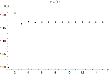
Figure 1: Convergence of the sequence $\left\{b_{k}\right\}_{k}$, for $\tau=0.1$ (left) and $\tau=0.5$ (right).

This leads to a cubic equation in $b_{\infty}$, but only one of the three solutions satisfies

$$b_{\infty}(A,\tau)\xrightarrow{\tau\to 0}1,$$

hence we uniquely identify our solution for $b_{\infty}(A,\tau)$. Explicitly:

$$b_{\infty}(A,\tau)=\frac{1+\frac{2\tau}{A}\left(1+\frac{\tau}{12}\right)+\sqrt{1+\frac{4\tau}{A}\left(1+\frac{\tau}{12}\right)}}{2\left(1+\frac{\tau}{12}\right)^{2}}.$$ (2.23)

The small coupling region is defined by the condition $Ab_{\infty}<\pi^{2}$, whence the critical value for the coupling is

$$A_{cr}(\tau)=\pi^{2}\left(1-\tau\left(\frac{1}{\pi^{2}}-\frac{1}{12}\right)\right)^{2},$$ (2.24)

as long as $\tau<\frac{12\pi^{2}}{12-\pi^{2}}$, and no positive solution for $\tau$ bigger than the mentioned value. At this point, we ought to check the consistency of our initial assumption: we developed a perturbative expansion in $\tau$, and then solved it to all orders, assuming the existence of a region $A>A_{lb}$ for which

$$\tau\left(\frac{1}{Ab_{\infty}}-\frac{1}{12}\right)<1,$$

corresponding to:

$$Ab_{\infty}(A,\tau)>\frac{12\tau}{12+\tau}.$$ (2.25)

As we have the explicit expression for $b_{\infty}(A,\tau)$, we can see that the infimum of the left hand side of (2.25), as a function of $A$ is exactly the right hand side, that is, $b_{\infty}$ takes exactly the expression for which the lower bound is pushed to $A_{lb}=0$. This means that our procedure holds for any $A>0,\tau\geq 0$, or, in other words, the assumption we made to start with the perturbative procedure is always verified in the region of validity of the heat kernel expansion.

To summarize, we have proved that, after the $T\overline{T}$-deformation, we still have a small coupling phase $0<A<A_{cr}(\tau)$ analogous to the undeformed case, with eigenvalue distribution given by a Wigner semicircle. Nevertheless, the effect of the deformation is to modify the parameter of the distribution, as well as moving the original critical value Douglas:1993iia . In particular, for small values of $\tau$, the value $A_{cr}(\tau)$ of the critical area is a decreasing function, hence $A_{cr}\leq\pi^{2}$, whilst when $\tau\geq\frac{12\pi^{2}}{12-\pi^{2}}$ we do not have any small coupling phase, due to the constraint $A>0$, and only the strong coupling phase exists. The eigenvalue density in the small coupling phase $0<A<A_{cr}(\tau)$ is:

$$\rho(h)=\frac{Ab_{\infty}(A,\tau)}{2\pi}\sqrt{\frac{4}{Ab_{\infty}(A,\tau)}-h^{2}},\qquad\mathrm{supp}\rho=\left[-\frac{2}{\sqrt{Ab_{\infty}(A,\tau)}},\frac{2}{\sqrt{Ab_{\infty}(A,\tau)}}\right],$$ (2.26)

where $b_{\infty}(A,\tau)$ is given in (2.23).

2.2 Strong coupling phase

Throughout the solution showed above, we had to impose an upper bound to the coupling $A$ in order not to violate the constraint (2.10). When $A>A_{cr}(\tau)$ the Wigner semicircle distribution is not allowed anymore, so that we have to look for a two-cut solution of the saddle point equation (2.11). We follow again a perturbative approach, reproducing the procedure of Douglas:1993iia order by order. According to what we have seen in the small coupling phase, the $T\overline{T}$-deformation introduces a nontrivial dependence on the parameters $A$ and $\tau$, but preserves the form of the Douglas–Kazakov solution. Therefore the two-cut solution, if any, must be of the form:

$$\rho(h)=\begin{cases}\varphi(h),\quad h\in\left[-\alpha,-\beta\right]\cup\left[\beta,\alpha\right],\\ 1,\quad\quad\ \ h\in\left[-\beta,\beta\right],\end{cases}$$

where $0\leq\beta\leq\alpha$ depend, in general, on $A$ and $\tau$. Plugging this expression into (2.11) we get:

$$\mathrm{P}\int du\frac{\varphi(u)}{h-u}=\log\left(\frac{h-b}{h+b}\right)+\frac{A}{2}h\sum_{j=0}^{\infty}\left(j+1\right)\tau^{j}\left[\int du\rho(u)u^{2}-\frac{1}{12}\right]^{j}.$$ (2.27)

The idea is again to proceed perturbatively in $\tau$, evaluating the second moment on the right hand side, using the approximation at previous order. Again, this will only account for a modification $A\mapsto Ad_{k}$, with

$$d_{k}=\sum_{j=0}^{k}\left(j+1\right)\tau^{j}\left[\int_{-\alpha}^{\alpha}du\rho(u)u^{2}-\frac{1}{12}\right]^{j},$$ (2.28)

where the second moment of the distribution is evaluated at order $k-1$.

We directly treat the problem at a generic order $k$, knowing that $d_{0}=1$, and hence the initial step of our procedure corresponds to the result of Douglas:1993iia . We define a complex function

$$\Phi(z)=\int\frac{\varphi(u)}{u-z}du,$$ (2.29)

for $z\notin\left[-\alpha,\alpha\right]$. On one hand, when $z$ approaches a real number $h\in\left[-\alpha,\alpha\right]$, we can write

$$\Phi_{+}\left(h\right)-\Phi_{-}\left(h\right)=2\pi\mathrm{i}\varphi(h)1\!\!1_{U}(h),$$ (2.30)

where $\Phi_{\pm}(h):=\lim_{\varepsilon\rightarrow 0}\Phi\left(h\pm\mathrm{i}\varepsilon\right)$ and $1\!\!1_{U}$ is the characteristic function of the set

$$U:=\left[-\alpha,-\beta\right]\cup\left[\beta,\alpha\right]\equiv\left[-\alpha,\alpha\right]\setminus\left(-\beta,\beta\right).$$

Once we obtain a complex solution to the saddle point equation (2.27), we can recover the $\varphi$ by evaluating the left hand side of (2.30) as the discontinuity at the branch cut of the complex solution for $h\in\left[-\alpha,\alpha\right]$. Such a complex solution is:

$$\Phi(z)=-\frac{1}{2\pi\mathrm{i}}\sqrt{\left(\alpha^{2}-z^{2}\right)\left(\beta^{2}-z^{2}\right)}\oint_{\gamma_{U}}du\frac{\frac{Ad_{k}}{2}u+\log\left(\frac{u-\beta}{u+\beta}\right)}{\left(u-z\right)\sqrt{\left(\alpha^{2}-u^{2}\right)\left(\beta^{2}-u^{2}\right)}},$$ (2.31)

for some path $\gamma_{U}$ in the complex plane around the cut $U$. After an adequate deformation of the contour integral, one gets:

$$\Phi(z)=-\frac{Ad_{k}}{2}z-\log\left(\frac{z-\beta}{z+\beta}\right)-\sqrt{\left(\alpha^{2}-z^{2}\right)\left(\beta^{2}-z^{2}\right)}\int_{-\beta}^{\beta}\frac{du}{\left(u-z\right)\sqrt{\left(\alpha^{2}-u^{2}\right)\left(\beta^{2}-u^{2}\right)}}.$$ (2.32)

The first two terms are obtained from the residue theorem, and the last one accounts for the branch cut of the logarithm along $\left[-\beta,\beta\right]$. When $z$ approaches the real axis, the logarithm has a discontinuity of $2\pi\mathrm{i}$ if $z\rightarrow h\in\left[-\beta,\beta\right]$, and has no discontinuity out of that interval, while the third term is discontinuous in all $z\in\left[-\alpha,\alpha\right]$. Thus we get:

$$\Phi_{+}\left(h\right)-\Phi_{-}\left(h\right)=-2\pi\mathrm{i}1\!\!1_{\left[-\beta,\beta\right]}-2\mathrm{i}\mathrm{sign}(h)\sqrt{\left(\alpha^{2}-h^{2}\right)\left(h^{2}-\beta^{2}\right)}\int_{-\beta}^{\beta}\frac{du}{\left(u-h\right)\sqrt{\left(\alpha^{2}-u^{2}\right)\left(\beta^{2}-u^{2}\right)}}.$$ (2.33)

The sign function appears because, for $h\in\left[\beta,\alpha\right]$, one approaches the branch cut of the square root from the proper direction, i.e. $\Phi_{+}-\Phi_{-}$ corresponds to “counter-clockwise minus clockwise”. For $h\in\left[-\alpha,-\beta\right]$, instead, the branch cut is approached from the converse direction.

Therefore, comparing with (2.30), one arrives to:

$$\rho(h) =\varphi(h)1\!\!1_{U}+1\!\!1_{\left[-\beta,\beta\right]}$$ (2.34)

$$=\frac{1}{\pi}\mathrm{sign}(h)\sqrt{\left(\alpha^{2}-h^{2}\right)\left(h^{2}-\beta^{2}\right)}\int_{-\beta}^{\beta}\frac{du}{\left(h-u\right)\sqrt{\left(\alpha^{2}-u^{2}\right)\left(\beta^{2}-u^{2}\right)}}.$$

It is easy to check that eigenvalue distribution in a positive function of $h$ in all $\left[-\alpha,\alpha\right]$ and is identically $1$ in the interval $\left[-\beta,\beta\right]$.

Until this point we simply reproduced the procedure of Douglas:1993iia , which applies also for our generalized case. Notice that the eigenvalue distribution $\rho$ apparently does not yield an explicit dependence on $Ad_{k}$; nevertheless, the parameters $\alpha,\beta$ will depend on it, and so will do $\rho$. The boundaries $\alpha,\beta$ can be fixed by the asymptotic expansion of $\Phi(z)$, for instance by comparison between (2.32) and the definition (2.29). From this latter we have:

$$\Phi(z) =-\frac{1}{z}\left(\int_{U}du\varphi(u)+\frac{1}{z^{2}}\int_{U}du\varphi(u)u^{2}+\dots\right)$$ (2.35)

$$=-\frac{1}{z}\left[\left(1-2\beta\right)+\frac{1}{z^{2}}\left(\int_{-\alpha}^{\alpha}du\rho(u)u^{2}-\frac{2}{3}\beta^{3}\right)+\dots\right].$$

On the other hand, the explicit expression (2.32) implies:

$$\Phi(z) =-\frac{Ad_{k}}{2}z-\log\left(1-\frac{2\beta}{z}+\dots\right)+z\left(1-\frac{\alpha^{2}+\beta^{2}}{2z^{2}}+\dots\right)\int_{-\beta}^{\beta}du\frac{\left[1+\frac{u^{2}}{z^{2}}+\frac{u^{4}}{z^{4}}+\dots\right]}{\sqrt{\left(\alpha^{2}-u^{2}\right)\left(\beta^{2}-u^{2}\right)}}$$ (2.36)

$$=z\left[-\frac{Ad_{k}}{2}z+\int_{-\beta}^{\beta}\frac{du}{\sqrt{\left(\alpha^{2}-u^{2}\right)\left(\beta^{2}-u^{2}\right)}}\right]+\frac{1}{z}\left[2\beta+\int_{-\beta}^{\beta}du\frac{u^{2}-\frac{\alpha^{2}+\beta^{2}}{2}}{\sqrt{\left(\alpha^{2}-u^{2}\right)\left(\beta^{2}-u^{2}\right)}}\right]+\mathcal{O}\left(\frac{1}{z^{3}}\right)$$

The comparison at $\mathcal{O}(z)$ imposes the constraint

$$\int_{-\beta}^{\beta}\frac{du}{\sqrt{\left(\alpha^{2}-u^{2}\right)\left(\beta^{2}-u^{2}\right)}}=\frac{Ad_{k}}{2}\quad\Longrightarrow\quad\alpha=\frac{4}{Ad_{k}}K\left(\frac{\beta}{\alpha}\right),$$ (2.37)

where $K\left(\cdot\right)$ is the complete elliptic integral of first kind. Analogously, from comparison at $\mathcal{O}(z^{-1})$ one gets the constraint:

$$2\beta-\frac{\alpha^{2}+\beta^{2}}{2}\int_{-\beta}^{\beta}\frac{du}{\sqrt{\left(\alpha^{2}-u^{2}\right)\left(\beta^{2}-u^{2}\right)}}+\int_{-\beta}^{\beta}\frac{u^{2}du}{\sqrt{\left(\alpha^{2}-u^{2}\right)\left(\beta^{2}-u^{2}\right)}}=-1+2\beta$$ (2.38)

$$\Longrightarrow\quad K\left(\frac{\beta}{\alpha}\right)\left[2E\left(\frac{\beta}{\alpha}\right)-\left(1-\frac{\beta^{2}}{\alpha^{2}}\right)K\left(\frac{\beta}{\alpha}\right)\right]=\frac{Ad_{k}}{4},$$

where $E\left(\cdot\right)$ is the complete elliptic integral of second kind, and we plugged in (2.37) to simplify the expression. The result is clearly the same as Douglas:1993iia , up to a rescaling $A\mapsto Ad_{k}$.

As we are interested in knowing the second moment of the distribution $\rho$, we may use $\mathcal{O}(z^{-3})$ of the expansion above to obtain the dependence of the integral expression on the other parameters. It leads to:

$$\int_{-\alpha}^{\alpha}du\rho(u)u^{2} =\int_{-\beta}^{\beta}du\frac{-u^{4}+\frac{\alpha^{2}+\beta^{2}}{2}u^{2}+\frac{\left(\alpha^{2}-\beta^{2}\right)^{2}}{8}}{\sqrt{\left(\alpha^{2}-u^{2}\right)\left(\beta^{2}-u^{2}\right)}}$$ (2.39)

$$=\frac{\left(\alpha^{2}-\beta^{2}\right)^{2}}{16}Ad_{k}+\alpha\left(\alpha^{2}+\beta^{2}\right)\left[K\left(\frac{\beta}{\alpha}\right)-E\left(\frac{\beta}{\alpha}\right)\right]$$

$$-\frac{2}{3}\alpha^{3}\left[\left(2+\frac{\beta^{2}}{\alpha^{2}}\right)K\left(\frac{\beta}{\alpha}\right)-2\left(1+\frac{\beta^{2}}{\alpha^{2}}\right)E\left(\frac{\beta}{\alpha}\right)\right].$$

We can use the properties of the elliptic integrals to extract information about the dependence on $Ad_{k}$. In particular, from the first two conditions (2.37)-(2.38) we get that, for $Ad_{k}\rightarrow\pi^{2}$, one recovers the same parameters as approaching the critical point from below, that is, $\left(\alpha=2/\pi,\beta=0\right)$. More specifically, for $Ad_{k}$ close to $\pi^{2}$, we may approximate the elliptic integrals, and obtain the first terms of the expansion of $\alpha$ and $\beta$ around $Ad_{k}=\pi^{2}$:

$$\alpha =\frac{1}{\pi}\left[2-\frac{Ad_{k}-\pi^{2}}{\pi^{2}}+\frac{5}{4}\left(\frac{Ad_{k}-\pi^{2}}{\pi^{2}}\right)^{2}+\dots\right],$$ (2.40)

$$\beta =\frac{1}{\pi}\left[2\sqrt{2}\left(\frac{\left(Ad_{k}-\pi^{2}\right)}{\pi^{2}}\right)^{\frac{1}{2}}-\frac{15}{4\sqrt{2}}\left(\frac{Ad_{k}-\pi^{2}}{\pi^{2}}\right)^{\frac{3}{2}}+\dots\right].$$

Moreover, concerning the second moment, approximated close to the critical point, we get:

$$\int_{-\alpha}^{\alpha}du\rho(u)u^{2}=\frac{1}{\pi^{2}}\left[1-\frac{Ad_{k}-\pi^{2}}{\pi^{2}}+3\left(\frac{Ad_{k}-\pi^{2}}{\pi^{2}}\right)^{2}+\dots\right].$$ (2.41)

At this point, we are able to determine the full nonperturbative expression for the eigenvalue density $\rho(h)$, close enough to the critical point. That is: on one hand, we have a formal recursive expression for the coefficients $d_{k}$ of the perturbative expansion in $\tau$ at strong coupling, while on the other hand, if we want to determine the order of the phase transition, we need to know an explicit expression for the dependence of the eigenvalue density on the parameters $A$ and $\tau$. Notice however, that local information close to the critical point is enough to characterize the phase transition. For these reasons, we look for a full (nonperturbative) solution, approximating close to the critical point. The solution we will find will be only valid up to order $(Ad_{\infty}-\pi^{2})^{2}$.

The formal limit $k\rightarrow\infty$ of this expression (2.28) leads to the equation:

$$d_{\infty}=\left[1-\tau\left(\int_{-\alpha}^{\alpha}du\rho(u)u^{2}-\frac{1}{12}\right)\right]^{-2},$$ (2.42)

and the approximated solution close to the critical point is found plugging expression (2.41), obtaining:

$$d_{\infty}\approx\left[1-\tau\left[\frac{1}{\pi^{2}}\left(1-\frac{Ad_{\infty}-\pi^{2}}{\pi^{2}}\right)-\frac{1}{12}\right]\right]^{-2},$$ (2.43)

which again admits only one solution compatible with $\lim_{\tau\rightarrow 0}d_{\infty}\left(A,\tau\right)=1$. As a side remark, we highlight that the defining equation for $d_{\infty}$ starts to differ from the one for $b_{\infty}$ only at order $(Ad_{\infty}-\pi^{2})^{2}$, implying that $b_{\infty}$ and $d_{\infty}$ will coincide up to the first derivative when evaluated at the critical point $A_{cr}$ (same $1$-jet at $A_{cr}$).

2.3 Third order phase transition

In this subsection, we study the free energy from the point of view of small and large area, that is $A<A_{cr}\left(\tau\right)$ and $A>A_{cr}\left(\tau\right)$ respectively, with the aim to determine the order of the phase transition. The free energy of the system is defined as:

$$\mathcal{F}_{N}\left(A,\tau\right)=-\frac{1}{N^{2}}\mathcal{Z}_{N}\left(A,\tau\right).$$ (2.44)

In the large $N$ limit the derivative with respect to the control parameter $A$ is given by:

$$\frac{\partial\mathcal{F}}{\partial A}=\frac{1}{2}\sum_{j=0}^{\infty}\tau^{j}\left[\int du\rho(u)u^{2}-\frac{1}{12}\right]^{j+1}.$$ (2.45)

Before passing to the direct evaluation, we notice that:

$$\frac{\partial\mathcal{F}}{\partial A}=F_{\mathrm{DK}}^{\prime}\left(Ac_{\infty}\right)\sum_{j=0}^{\infty}\tau^{j}\left[\int du\rho(u)u^{2}-\frac{1}{12}\right]^{j},$$ (2.46)

where by ${F}_{\mathrm{DK}}^{\prime}(A)$ we mean the first derivative of the free energy obtained by Douglas and Kazakov Douglas:1993iia , and $c_{\infty}$ is a shorthand:

$$c_{\infty}=\begin{cases}b_{\infty},\quad A<A_{cr}(\tau);\\ d_{\infty},\quad A>A_{cr}(\tau).\end{cases}$$

Therefore

$$\frac{\partial\mathcal{F}}{\partial A}={F}_{\mathrm{DK}}^{\prime}(Ac_{\infty})\left[1-\tau\left(\int du\rho(u)u^{2}-\frac{1}{12}\right)\right]^{-1}.$$ (2.47)

Taking advantage of the defining equation (2.22) and (2.42) for $b_{\infty}$ and $d_{\infty}$ respectively, we can rewrite:

$$\frac{\partial\mathcal{F}}{\partial A}={F}_{\mathrm{DK}}^{\prime}(Ac_{\infty})\sqrt{c_{\infty}}.$$ (2.48)

When $A<A_{cr}$, the latter expression is calculated using the distribution at small coupling:

$$\frac{\partial\mathcal{F}}{\partial A}\bigg{|}_{A<A_{cr}}=\frac{\sqrt{b_{\infty}}}{2}\left(\frac{1}{Ab_{\infty}}-\frac{1}{12}\right)=\frac{\sqrt{b_{\infty}}}{2}\left[\frac{1}{\pi^{2}}\left(1-\frac{Ab_{\infty}-\pi^{2}}{\pi^{2}}+\left(\frac{Ab_{\infty}-\pi^{2}}{\pi^{2}}\right)^{2}+\dots\right)-\frac{1}{12}\right].$$ (2.49)

Analogously, in the strong coupling phase $A>A_{cr}(\tau)$ we ought to use the eigenvalue distribution at strong coupling, which, approximating close to the critical point, provides the expression:

$$\frac{\partial\mathcal{F}}{\partial A}\bigg{|}_{A>A_{cr}}=\frac{\sqrt{d_{\infty}}}{2}\left[\frac{1}{\pi^{2}}\left(1-\frac{Ad_{\infty}-\pi^{2}}{\pi^{2}}+3\left(\frac{Ad_{\infty}-\pi^{2}}{\pi^{2}}\right)^{2}+\dots\right)-\frac{1}{12}\right].$$

By construction of the two-cut solution, we know that:

$$Ab_{\infty}\xrightarrow{\ A\to A_{cr}^{-}\ }\pi^{2}\xleftarrow{\ A\to A_{cr}^{+}\ }Ad_{\infty}$$ (2.50)

which guarantees $\frac{\partial\mathcal{F}}{\partial A}$ is continuous at the critical point, thus the transition is at least of second order. We in fact have that:

$$\frac{\partial\mathcal{F}}{\partial A}\bigg{|}_{A>A_{cr}}-\frac{\partial\mathcal{F}}{\partial A}\bigg{|}_{A<A_{cr}} =\frac{1}{2}\left(\frac{1}{\pi^{2}}-\frac{1}{12}\right)\left(\sqrt{d_{\infty}}-\sqrt{b_{\infty}}\right)$$ (2.51)

$$-\frac{1}{2\pi^{2}}\left[\sqrt{d_{\infty}}\left(\frac{Ad_{\infty}-\pi^{2}}{\pi^{2}}\right)-\sqrt{b_{\infty}}\left(\frac{Ab_{\infty}-\pi^{2}}{\pi^{2}}\right)\right]$$

$$+\frac{1}{2\pi^{2}}\left[3\sqrt{d_{\infty}}\left(\frac{Ad_{\infty}-\pi^{2}}{\pi^{2}}\right)^{2}-\sqrt{b_{\infty}}\left(\frac{Ab_{\infty}-\pi^{2}}{\pi^{2}}\right)^{2}\right]+\dots.$$

Taking a further derivative with respect to $A$ we get:

$$\frac{\partial^{2}\mathcal{F}}{\partial A^{2}}\bigg{|}_{A>A_{cr}}-\frac{\partial^{2}\mathcal{F}}{\partial A^{2}}\bigg{|}_{A<A_{cr}} =\frac{1}{4}\left(\frac{1}{\pi^{2}}-\frac{1}{12}\right)\left[\frac{d_{\infty}^{\prime}}{\sqrt{d_{\infty}}}-\frac{b_{\infty}^{\prime}}{\sqrt{b_{\infty}}}\right]$$ (2.52)

$$-\frac{1}{4\pi^{2}}\left[\frac{d_{\infty}^{\prime}}{\sqrt{d_{\infty}}}\left(\frac{Ad_{\infty}-\pi^{2}}{\pi^{2}}\right)-\frac{b_{\infty}^{\prime}}{\sqrt{b_{\infty}}}\left(\frac{Ab_{\infty}-\pi^{2}}{\pi^{2}}\right)\right]$$

$$-\frac{1}{2\pi^{4}}\left[\sqrt{d_{\infty}}\left(d_{\infty}+Ad_{\infty}^{\prime}\right)-\sqrt{b_{\infty}}\left(b_{\infty}+Ab_{\infty}^{\prime}\right)\right]$$

$$+\frac{1}{4\pi^{2}}\left[3\frac{d_{\infty}^{\prime}}{\sqrt{d_{\infty}}}\left(\frac{Ad_{\infty}-\pi^{2}}{\pi^{2}}\right)^{2}-\frac{b_{\infty}^{\prime}}{\sqrt{b_{\infty}}}\left(\frac{Ab_{\infty}-\pi^{2}}{\pi^{2}}\right)^{2}\right]$$

$$+\frac{1}{\pi^{4}}\left[\sqrt{d_{\infty}}\left(d_{\infty}+Ad_{\infty}^{\prime}\right)\left(\frac{Ad_{\infty}-\pi^{2}}{\pi^{2}}\right)-\sqrt{b_{\infty}}\left(b_{\infty}+Ab_{\infty}^{\prime}\right)\left(\frac{Ab_{\infty}-\pi^{2}}{\pi^{2}}\right)\right]+\dots$$

Is is straightforward to see that the second, fourth and fifth term vanish at the critical point. The first and third term are more subtle, because the involve derivatives of the coefficients $b_{\infty},d_{\infty}$. However, we have that both coefficients are defined by formally the same expression, but using the eigenvalue distribution at small or large coupling respectively. Regarding $b_{\infty}$, we can evaluate its derivative using (2.22):

$$b_{\infty}^{\prime}=-\frac{2\tau}{\pi^{2}}\frac{b_{\infty}^{5/2}}{1-Ab_{\infty}^{3/2}}+\dots,$$

where the dots represent term that vanish at the critical point. The same can be done for $d_{\infty}$ using (2.42), to obtain:

$$d_{\infty}^{\prime}=-\frac{2\tau}{\pi^{2}}\frac{d_{\infty}^{5/2}}{1-Ad_{\infty}^{3/2}}+\dots.$$

Hence we infer that the first derivatives $b_{\infty}^{\prime}$ and $d_{\infty}^{\prime}$ of the coefficients coincide at the critical point (this fails to be true for higher derivatives). Consequently, the phase transition is again of third order.

It is remarkable that the $T\overline{T}$-deformation introduced a nontrivial dependence on the coupling $A$, but in such a way that it does not affect the order of the phase transition.

3 Instanton analysis

Gross and Matytsin presented evidence for the phase transition to be triggered by instantons Gross:1994mr . The existence of a phase transition can be closely related to the discreteness of the matrix model (1.3) Gross:1994mr ; Jafferis:2005jd ; Szabo:2013vva . In Minahan:1993tp , Yang–Mills theory on the sphere is described in terms of $N$ nonrelativistic free fermions on $\operatorname{\mathbb{S}}^{1}$, with instantons corresponding to different winding numbers for fermions at a given position, and the phase transition occurs due to the condensation of fermions in (discrete) momentum space, so again the discreteness turned out to be essential to permit a phase transition. From this general argument, and taking into account expression (2.1), the statement is expected to hold also in the $T\overline{T}$-deformed version of two-dimensional Yang–Mills, as the effect of the deformation, at the level of the matrix model, is to replace the discrete Gaussian weight with a discrete weight whose potential has also additional multitrace contributions. Thus, in this section we look at the role played by instantons in the phase transition.

3.1 Instantons in the undeformed theory

By instanton, we mean a solution of the classical Yang–Mills equation of motion which is gauge inequivalent to the trivial one. Those solutions are in one to one correspondence with collections of $N$ monopole charges:

$$\ell:=\left(\ell_{1},\dots,\ell_{N}\right)\in\operatorname{\mathbb{Z}}^{N}.$$

The action for a given classical configuration is:

$$S_{inst}\left(\ell\right)=\frac{N}{2A}\sum_{j=1}^{N}\left(2\pi\ell_{j}\right)^{2},$$ (3.1)

and the partition function splits into the sum of contributions from instanton sectors:

$$\mathcal{Z}_{N}^{(\mathrm{YM})}=\sum_{\ell\in\operatorname{\mathbb{Z}}^{N}}w\left(\ell\right)e^{-S_{inst}\left(\ell\right)}.$$ (3.2)

This is the content of Witten’s result Witten:1991we ; Witten:1992xu extending the Duistermaat–Heckman theorem. From the point of view of the Abelianization procedure Blau:1993tv , each $\ell_{j}$ is the first Chern class of a $U(1)$-bundle. See Blau:1993tv ; Blau:1993hj ; Cordes:1994fc for more details. Later on, this viewpoint was the one adopted in Jafferis:2005jd to estimate the instanton contributions in the case of $q$-deformed Yang–Mills theory on $\operatorname{\mathbb{S}}^{2}$.

A practical difficulty is to evaluate the weights $w\left(\ell\right)$, which was done in Minahan:1993tp (and in Caporaso:2005ta for the $q$-deformed case), through the method of Poisson resummation. In Gross:1994mr , the contribution of the single-monopole sector $\ell=\left(1,0,\dots,0\right)$ was calculated, showing that this correction to the saddle point approximation at large $N$ is exponentially suppressed,

$$\frac{w\left(1,0,\dots,0\right)e^{-S_{inst}\left(1,0,\dots,0\right)}}{w\left(0,\dots,0\right)e^{-S_{inst}\left(0,\dots,0\right)}}\propto e^{-\frac{2\pi^{2}}{A}N\gamma\left(\frac{A}{\pi^{2}}\right)},$$

where the function $\gamma\left(\cdot\right)$ is the one introduced by Gross and Matytsin Gross:1994mr and is given by

$$\gamma(x)=\sqrt{1-x}-\frac{x}{2}\log\left(\frac{1+\sqrt{1-x}}{1-\sqrt{1-x}}\right).$$ (3.3)

In particular, as $\gamma\left(x\right)>0$ for $0<x<1$ and $\gamma\left(1\right)=0$, in the small coupling phase contributions from instanton sectors are exponentially suppressed at large $N$, but they become more and more relevant as the critical point is approached. In this sense, the weight $w\left(\ell\right)$ acts as a counterpart of the Boltzmann factor $e^{-S\left(\ell\right)}$, and at the critical point those two contributions are exactly balanced.

3.2 Instantons in the $T\overline{T}$-deformed theory

The evaluation of the full instanton expansion for the deformed theory would correspond to find an explicit expression of the form:

$$\mathcal{Z}_{N}\left(A,\tau\right)=\sum_{\ell\in\operatorname{\mathbb{Z}}^{N}}w\left(\ell\right)e^{-S_{inst}\left(\ell\right)},$$

where now the weights and the action include the effects of the deformation by the $T\overline{T}$-operator. We have found strong evidence that this can be done in an analytic way, but the weights obtained are not very enlightening and unsuitable for the purpose of this section. Instead, we will only look at the first instanton correction, and how it affects the model. A discussion on the Poisson resummation for the full explicit expression is relegated to Appendix A.

As a first step, the partition function can be rewritten as a sum over Fourier transforms of contributions from each representation:

$$\mathcal{Z}_{N}\left(A,\tau\right)=\sum_{\ell\in\operatorname{\mathbb{Z}}^{N}}Z_{\ell},$$ (3.4)

where each instanton sector contributes as:

$$Z_{\ell}=\int_{\operatorname{\mathbb{R}}^{N}}\prod_{i=1}^{N}dh_{i}e^{-\mathrm{i}2\pi\sum_{i=1}^{N}\ell_{i}h_{i}}\prod_{i<j}\left(\frac{h_{i}-h_{j}}{j-i}\right)^{2}e^{-\frac{A}{2N}\sum_{j=0}^{\infty}\left(\frac{\tau}{N^{3}}\right)^{j}\left(\sum_{i=1}^{N}h_{i}^{2}-\frac{N\left(N^{2}+2\right)}{12}\right)^{j+1}}.$$ (3.5)

Consider the single-monopole sector corresponding to $\ell=\left(\ell_{1},0,\dots,0\right)$ (we will eventually set $\ell_{1}=\pm 1$). It contributes to the partition function as:

$$Z_{\left(\ell_{1},0,\dots,0\right)}=\int_{\operatorname{\mathbb{R}}^{N}}\prod_{i=1}^{N}dh_{i}e^{-N^{2}S_{\ell_{1}}[h]},$$

where

$$S_{\ell_{1}}[h]=-\frac{2}{N^{2}}\sum_{i<j}\log\left(\frac{h_{i}-h_{j}}{j-i}\right)+\frac{A}{2N^{3}}\sum_{j=0}^{\infty}\left(\frac{\tau}{N^{3}}\right)^{j}\left(\sum_{i=1}^{N}h_{i}^{2}-\frac{N\left(N^{2}+2\right)}{12}\right)^{j+1}+\frac{2\pi\mathrm{i}}{N^{2}}\ell_{1}h_{1}.$$ (3.6)

This means that the correction to the large $N$ action, with respect to the vacuum sector, is of $\mathcal{O}(N^{-1})$. This implies that, at large $N$, we can perform $N-1$ integrals using the saddle point approximation for the eigenvalue distribution, and eventually treat the integration over $h_{1}$ separately Gross:1994mr ; Jafferis:2005jd . Notice that the saddle point for $h_{1}$ will be, in general, complex, due to the purely imaginary “Fourier interaction” with $\ell_{1}$. Nevertheless, as we are interested in the suppressing factor, we will avoid the technicalities involved in determining the imaginary part of the instanton contribution.

Taking the large $N$ limit, we have:

$$Z_{\left(\ell_{1},0,\dots,0\right)}=\mathcal{C}^{N-1}\int_{-\infty}^{\infty}dh_{1}e^{-NS_{\ell_{1}}[h_{1}]},$$ (3.7)

where $\mathcal{C}$ is the integral over any variable $h_{2},\dots,h_{N}$, calculated with the saddle point approximation, and the effective action for the scaled variable $h=\frac{h_{1}}{N}$ is:

$$S_{\ell_{1}}[h]=-2\int du\rho(u)\log\left(h-u\right)-2+\frac{A}{2}\sum_{j=0}^{\infty}\tau^{j}\left(h^{2}-\frac{1}{12}\right)^{j+1}+2\pi\mathrm{i}\ell_{1}h,$$ (3.8)

and the density $\rho$ is the one obtained in (2.26) for small coupling $A<A_{cr}$. The saddle point for the effective action is given by:

$$2\mathrm{P}\int du\frac{\rho(u)}{h-u}+Ah\sum_{j=0}^{\infty}\left(j+1\right)\tau^{j}\left(h^{2}-\frac{1}{12}\right)^{j}+2\pi\mathrm{i}\ell_{1}=0$$

which, using the fact that $\rho$ satisfies the saddle point for $\ell_{1}=0$, simplifies into:

$$2\pi\mathrm{i}\left(\rho(h)+\ell_{1}\right)=0.$$

This leads to the saddle point:

$$h^{2}=\left(\frac{2}{Ab_{\infty}}\right)^{2}\left(Ab_{\infty}-\pi^{2}\ell_{1}\right),$$

which, since the analysis is being brought on in the small coupling phase $Ab_{\infty}<\pi^{2}$, gives a purely imaginary saddle point:

$$h=\frac{2\pi\mathrm{i}}{Ab_{\infty}}\mathrm{sign}(\ell_{1})\sqrt{\ell_{1}^{2}-\frac{Ab_{\infty}}{\pi^{2}}}.$$ (3.9)

The result is exactly the same obtained in the undeformed case Gross:1994mr , up to a rescaling $A\mapsto Ab_{\infty}$. In particular:

$$\frac{Z_{\left(1,0,\dots,0\right)}}{Z_{\left(0,\dots,0\right)}}=\mathcal{C}^{\prime}e^{-N\frac{2\pi^{2}}{Ab_{\infty}}\gamma\left(\frac{Ab_{\infty}}{\pi^{2}}\right)},$$ (3.10)

where $\mathcal{C}^{\prime}$ is an overall constant and $\gamma\left(\cdot\right)$ is the function (3.3). Hence, the same conclusions of the undeformed case Gross:1994mr hold: from the perspective of the small coupling expansion, the phase transition is triggered by instantons.

A more thorough analysis of the single-monopole instanton correction in the $T\overline{T}$-deformed case, shows that the relevance of instantons increases with $\tau$, for $\tau<\frac{12\pi^{2}}{12-\pi^{2}}$, and there is no suppression at all for $\tau\geq\frac{12\pi^{2}}{12-\pi^{2}}$. This explains why the phase transition occurs earlier in the deformed case, that is $A_{cr}(\tau)\leq A_{cr}(0)$: indeed, the function $\frac{1}{Ab_{\infty}}\gamma\left(\frac{Ab_{\infty}}{\pi^{2}}\right)$ decreases faster than the function $\frac{1}{A}\gamma\left(\frac{A}{\pi^{2}}\right)$, hence the first instanton sector becomes relevant at a lower value of $A$, in comparison to the undeformed case. This is presented in Figures 2 and 3.

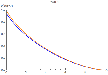
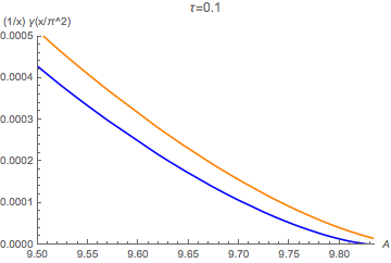
Figure 2: On the left: a comparison of the function $\gamma\left(\frac{x}{\pi^{2}}\right)$ for the deformed (blue) and undeformed (orange) case. On the right: a zoom on the tail of the function $\frac{1}{x}\gamma\left(\frac{x}{\pi^{2}}\right)$ for the deformed (blue) and undeformed (orange) case. The plots are at $\tau=0.1$.

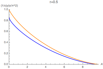
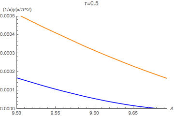
Figure 3: On the left: a comparison of the function $\gamma\left(\frac{x}{\pi^{2}}\right)$ for the deformed (blue) and undeformed (orange) case. On the right: a zoom on the tail of the function $\frac{1}{x}\gamma\left(\frac{x}{\pi^{2}}\right)$ for the deformed (blue) and undeformed (orange) case. The plots are at $\tau=0.5$.

4 Outlook

It is worth mentioning a few possible open problems, from the point of view of classical results involving two-dimensional Yang–Mills theory on the sphere. One is the study of Wilson loops, a well-known solvable problem in the undeformed theory. Some results in this regard are immediately available by using some of the results above. Recall that already the zero instanton sector of ordinary two-dimensional Yang–Mills theory is well-known to capture the vacuum expectation value of Wilson loops in $4d$ $\mathcal{N}=4$ supersymmetric Yang–Mills theory Giombi:2009ds ; Giombi:2009ek . The zero instanton sector of the ordinary theory is described by a Gaussian matrix model and hence, the Wilson loop average in that ensemble is the well-known Bassetto:1998sr ; Drukker:2000rr

$$\left\langle W_{0}\right\rangle=\frac{1}{N}\exp\left(-g^{2}\frac{A_{1}A_{2}}{2A}\right)L_{N-1}^{1}\left(g^{2}\frac{A_{1}A_{2}}{A}\right),$$ (4.1)

where $L_{N-1}^{1}(x)$ is a Laguerre polynomial.

We have obtained that the density of states in the weak coupling phase is given by a Wigner semicircle law with a rescaled parameter $A\mapsto Ab_{\infty}$. Hence the large $N$ Wilson loop in the zero-instanton sector of the $T\overline{T}$-deformed theory will be given by a rescaled version of the large $N$ limit of (4.1), which is given by a Bessel function, and has a celebrated dual holographic description Drukker:2000rr . Thus, it is interesting to carry out the analysis of the Wilson loops in the $T\overline{T}$-deformed theory and look for potential implications in supersymmetric gauge theory.

It is also worth mentioning that some results on Wilson loops in $2d$ Yang–Mills theory on the plane, in part to further understand the Duurhus–Olensen transition Durhuus:1980nb , precisely make use of the existence of a Burgers equation for certain generating functions (in the form of characteristic polynomials) of the Wilson loops Blaizot:2008nc ; Neuberger:2008ti . Since this property follows from the heat kernel propagator, which is preserved under the deformation, such methods and studies will seemingly translate to the deformed case as well.

Two-dimensional Yang–Mills theory has many other interesting aspects that could now be re-analyzed under the prism of the $T\overline{T}$-deformation of the theory. Clear examples are the factorization of the theory in chiral and anti-chiral sectors and the corresponding Gross–Taylor string theory interpretation in terms of branched covers, known for both the full theory and for a chiral sector Gross:1992tu ; Gross:1993hu ; Cordes:1994fc ; Donnelly:2016jet . In turn, already in the undeformed case, the interplay of all these aspects with the large $N$ phase transition is an interesting subject Crescimanno:1994eg . Another possibility could be to start with the generalized theory Douglas:1994pq ; Ganor:1994bq , which also includes the effect of higher-order Casimir operators or perhaps consider the theory with the presence of a topological $\theta$-term. These are well known aspects of the two-dimensional Yang–Mills theory that would possibly be interesting to inspect from the novel point of view of the $T\overline{T}$-deformation.

More recent developments, that nonetheless are already being investigated for over a decade, involve the $q$-deformation of the $2d$ Yang–Mills theory, which has been proven to enjoy a large number of relationships with topological strings, Chern–Simons theories and supersymmetric gauge theories in a number of dimensions (e.g. in the study of the $4d$ superconformal index Gadde:2011ik ). The partition function of $q$-deformed Yang–Mills theory on a Riemann surface $\Sigma_{h}$ is a straightforward variation of the Migdal formula, which involves quantum dimensions rather than ordinary dimensions of representations of the gauge group Aganagic:2004js :

$$\mathcal{Z}_{N,h}(q,p)=\sum_{R}\left(\dim_{q}R\right)^{2-2h}q^{\frac{p}{2}C_{2}\left(R\right)}.$$

This $q$-deformed gauge theory can be regarded as an analytic continuation of Chern–Simons gauge theory on a Seifert fibration of degree $p$ over the Riemann surface $\Sigma_{h}$. For genus $h=0$, the Seifert manifold is the three-sphere $\operatorname{\mathbb{S}}^{3}$ for $p=1$, regarded as the Hopf fibration $\operatorname{\mathbb{S}}^{3}\rightarrow\Sigma_{0}=\operatorname{\mathbb{S}}^{2}$, and the lens space $L(p,1)=\operatorname{\mathbb{S}}^{3}/\operatorname{\mathbb{Z}}_{p}$ for $p>1$. Localization results have been proved also for the $q$-deformed case Beasley:2005vf ; Kallen:2011ny (see also Caporaso:2005ta for explicit derivation in the case of the sphere).

Notice that, naively, the deformation is “complementary” to the $T\overline{T}$ deformation, as it involves only the dimensions part and not the Casimir part Szabo:2013vva . The problem of phase transitions in the $q$-deformed theory was studied, also following the classical works Douglas:1993iia ; Gross:1994mr , in Jafferis:2005jd ; Arsiwalla:2005jb ; Caporaso:2005ta .

Appendix A Instanton sectors and Poisson resummation

This appendix is dedicated to a more accurate calculation of the instanton contributions in the present model. We will follow the procedure of Minahan:1993tp to evaluate the weights $w\left(\ell\right)$ in the $T\overline{T}$-deformed version of the theory (2.1). The full instanton expansion is obtained starting from the formula

$$\mathcal{Z}_{N}\left(A,\tau\right)=\sum_{\ell\in\operatorname{\mathbb{Z}}^{N}}Z_{\ell},$$

where $Z_{\ell}$ is the Fourier transform of the sector corresponding to a given representation, that is,

$$Z_{\ell}=\int\prod_{i}dh_{i}e^{-2\pi\mathrm{i}\sum_{i}\ell_{i}h_{i}}\prod_{i<j}\left(\frac{h_{i}-h_{j}}{i-j}\right)^{2}e^{-\frac{A}{2N}\sum_{j=0}^{\infty}\left(\frac{\tau}{N^{3}}\right)^{j}\left[\sum_{i}\left(h_{i}-i+\frac{N}{2}\right)\left(h_{i}+i-\frac{N}{2}\right)\right]^{j+1}}.$$ (A.1)

We can expand the contribution arising from the $T\overline{T}$-deformation:

$$Z_{\ell}=\mathcal{C}\int \prod_{i}dh_{i}e^{-2\pi\mathrm{i}\sum_{i}\ell_{i}h_{i}}\prod_{i<j}\left(h_{i}-h_{j}\right)^{2}e^{-\frac{A}{2N}\sum_{i}h_{i}^{2}}$$ (A.2)

$$\times\left\{\sum_{n=0}^{\infty}\frac{1}{n!}\left(-\frac{A}{2N}\right)^{n}\sum_{j=0}^{\infty}c_{j}(n)\left(\frac{\tau}{N^{3}}\right)^{j}\left[\sum_{i}h_{i}^{2}-\frac{N(N^{2}-1)}{12}\right]^{j}\right\},$$

where $\mathcal{C}$ is an irrelevant overall factor and $\left\{c_{j}(n)\right\}_{j}$ are the coefficients of the series expansion of $\left(\frac{x}{1-x}\right)^{n}$. Neglecting the shift in the Casimir, and putting the focus on the last term, we obtain its Fourier transform as:

$$\int dh_{i}e^{-2\pi\mathrm{i}\ell_{i}h_{i}-\frac{A}{2N}h_{i}^{2}}\left[\frac{\tau}{N^{3}}h_{i}^{2}\right]^{j}=\left(\frac{\tau}{N^{3}}\right)^{j}\Gamma\left(\frac{1}{2}+{j}\right){{}_{1}F_{1}}\left(\frac{1}{2}+{j},\frac{1}{2},-\frac{N}{2A}\ell_{i}^{2}\right),$$

where ${{}_{1}F_{1}}$ is the confluent hypergeometric function.

The key observation to go further is that, inside the integral (A.2), three ingredients appear: the Gaussian measure, the Vandermonde determinant and a totally symmetric polynomial in the variables $h_{i}^{2}$. Therefore, performing the integration with a single Vandermonde determinant, which is a totally antisymmetric polynomial, one obtains again the Vandermonde multiplying some totally symmetric polynomial (or total symmetrisation of hypergeometric functions), up to overall constant factors. The result is indeed:

$$f_{1}\left(\ell\right):=\int\prod_{i}dh_{i}e^{-2\pi\mathrm{i}\sum_{i}\ell_{i}h_{i}-\frac{A}{2N}\sum_{i}h_{i}^{2}}\prod_{i<j}\left(h_{i}-h_{j}\right)\left\{\sum_{n=0}^{\infty}\frac{1}{n!}\left(-\frac{A}{2N}\right)^{n}\sum_{j=0}^{\infty}c_{j}(n)\left(\frac{\tau}{N^{3}}\right)^{j}\left[\sum_{i}h_{i}^{2}\right]^{j}\right\}$$

$$=\mathcal{C}^{\prime}\ \prod_{i<j}\left(\ell_{i}-\ell_{j}\right)e^{-\frac{N}{2A}\sum_{i}\ell_{i}^{2}}\sum_{n=0}^{\infty}\frac{1}{n!}\left(-\frac{A}{2N}\right)^{n}\sum_{j=0}^{\infty}c_{j}(n)\left(\frac{\tau}{N^{3}}\right)^{j}\mathcal{S}\left({{}_{1}F_{1}}\left(\frac{1}{2}+\nu_{i}+j,\frac{1}{2}+\tilde{\nu}_{i},-\frac{N}{2A}\ell_{i}^{2}\right)\right),$$

where $\mathcal{S}(x)$ is a totally symmetric polynomial of order $N$ in $N$ variables, and $\nu_{i},\tilde{\nu}_{i}\in\mathbb{N}$. Therefore, the arguments presented in Minahan:1993tp hold also in this case. Taking care of the polynomials that appear due to the $T\overline{T}$-deformation, and one could retrieve the exact form of $Z_{\ell}$, by taking the convolution of two expressions as given above

$$Z_{\ell}=\left(f_{1}\ast f_{1}\right)\left(\ell\right).$$

Although the discussion presented in this Appendix is qualitative, it illustrates how the exact instanton contribution should in principle be obtainable following standard methods. In particular, the shift in the quadratic Casimir can be reintroduced, and, using the binomial expansion, one can apply the calculations sketched here, taking care of the coefficients, to retrieve the exact contribution of each instanton sector.

References

- (1) A. B. Zamolodchikov, Expectation value of composite field T anti-T in two-dimensional quantum field theory, (2004) [hep-th/0401146].
- (2) F. A. Smirnov and A. B. Zamolodchikov, On space of integrable quantum field theories, Nucl. Phys. B915 (2017) 363 [1608.05499].
- (3) A. Cavaglià, S. Negro, I. M. Szécsényi and R. Tateo, -deformed 2D Quantum Field Theories, JHEP 10 (2016) 112 [1608.05534].
- (4) S. Dubovsky, V. Gorbenko and M. Mirbabayi, Asymptotic fragility, near AdS2 holography and , JHEP 09 (2017) 136 [1706.06604].
- (5) S. Dubovsky, V. Gorbenko and G. Hernández-Chifflet, Partition Function from Topological Gravity, JHEP 09 (2018) 158 [1805.07386].
- (6) A. Giveon, N. Itzhaki and D. Kutasov, and LST, JHEP 07 (2017) 122 [1701.05576].
- (7) A. Giveon, N. Itzhaki and D. Kutasov, A solvable irrelevant deformation of AdS3/CFT2, JHEP 12 (2017) 155 [1707.05800].
- (8) S. Datta and Y. Jiang, deformed partition functions, JHEP 08 (2018) 106 [1806.07426].
- (9) O. Aharony, S. Datta, A. Giveon, Y. Jiang and D. Kutasov, Modular invariance and uniqueness of deformed CFT, (2018) [1808.02492].
- (10) J. Cardy, The deformation of quantum field theory as random geometry, (2018) [1801.06895].
- (11) R. Conti, S. Negro and R. Tateo, The perturbation and its geometric interpretation, (2018) [1809.09593].
- (12) J. Cardy, deformations of non-Lorentz invariant field theories, (2018) [1809.07849].
- (13) R. Conti, L. Iannella, S. Negro and R. Tateo, Generalised Born-Infeld models, Lax operators and the perturbation, (2018) [1806.11515].
- (14) S. Cordes, G. W. Moore and S. Ramgoolam, Lectures on 2-d Yang-Mills theory, equivariant cohomology and topological field theories, Nucl. Phys. Proc. Suppl. 41 (1995) 184 [hep-th/9411210].
- (15) M. R. Douglas and V. A. Kazakov, Large N phase transition in continuum QCD in two-dimensions, Phys. Lett. B319 (1993) 219 [hep-th/9305047].
- (16) D. J. Gross and A. Matytsin, Instanton induced large N phase transitions in two-dimensional and four-dimensional QCD, Nucl. Phys. B429 (1994) 50 [hep-th/9404004].
- (17) A. A. Migdal, Recursion Equations in Gauge Theories, Sov. Phys. JETP 42 (1975) 413.
- (18) P. Menotti and E. Onofri, The Action of SU() Lattice Gauge Theory in Terms of the Heat Kernel on the Group Manifold, Nucl. Phys. B190 (1981) 288.
- (19) B. E. Rusakov, Loop averages and partition functions in U(N) gauge theory on two-dimensional manifolds, Mod. Phys. Lett. A5 (1990) 693.
- (20) M. R. Douglas, Conformal field theory techniques in large N Yang-Mills theory, NATO Advanced Research Workshop on New Developments in String Theory, Conformal Models and Topological Field Theory Cargese, France (1993) [hep-th/9311130].
- (21) J. A. Minahan and A. P. Polychronakos, Classical solutions for two-dimensional QCD on the sphere, Nucl. Phys. B422 (1994) 172 [hep-th/9309119].
- (22) D. J. Gross and E. Witten, Possible Third Order Phase Transition in the Large N Lattice Gauge Theory, Phys. Rev. D21 (1980) 446.
- (23) S. R. Wadia, = Infinity Phase Transition in a Class of Exactly Soluble Model Lattice Gauge Theories, Phys. Lett. 93B (1980) 403.
- (24) M. Caselle, A. D’Adda, L. Magnea and S. Panzeri, Two-dimensional QCD on the sphere and on the cylinder, Proceedings, Summer School in High-energy physics and cosmology: Trieste, Italy (1993) 0245 [hep-th/9309107].
- (25) D. J. Gross, Two-dimensional QCD as a string theory, Nucl. Phys. B400 (1993) 161 [hep-th/9212149].
- (26) D. J. Gross and W. Taylor, Two-dimensional QCD is a string theory, Nucl. Phys. B400 (1993) 181 [hep-th/9301068].
- (27) W. Donnelly and G. Wong, Entanglement branes in a two-dimensional string theory, JHEP 09 (2017) 097 [1610.01719].
- (28) A. C. Pipkin, A Course on Integral Equations, no. 9 in Texts in Applied Mathematics. Springer-Verlag, 1991.
- (29) N. I. Muskhelishvili, Singular Integral Equations. Noordhoff, 1977.
- (30) D. Jafferis and J. Marsano, A DK phase transition in q-deformed Yang-Mills on S**2 and topological strings, (2005) [hep-th/0509004].
- (31) R. J. Szabo and M. Tierz, q-deformations of two-dimensional Yang-Mills theory: Classification, categorification and refinement, Nucl. Phys. B876 (2013) 234 [1305.1580].
- (32) E. Witten, On quantum gauge theories in two-dimensions, Commun. Math. Phys. 141 (1991) 153.
- (33) E. Witten, Two-dimensional gauge theories revisited, J. Geom. Phys. 9 (1992) 303 [hep-th/9204083].
- (34) M. Blau and G. Thompson, Derivation of the Verlinde formula from Chern-Simons theory and the G/G model, Nucl. Phys. B408 (1993) 345 [hep-th/9305010].
- (35) M. Blau and G. Thompson, Lectures on 2-d gauge theories: Topological aspects and path integral techniques, Proceedings, Summer School in High-energy physics and cosmology: Trieste, Italy (1993) 0175 [hep-th/9310144].
- (36) N. Caporaso, M. Cirafici, L. Griguolo, S. Pasquetti, D. Seminara and R. J. Szabo, Topological strings and large N phase transitions. I. Nonchiral expansion of q-deformed Yang-Mills theory, JHEP 01 (2006) 035 [hep-th/0509041].
- (37) S. Giombi and V. Pestun, Correlators of local operators and 1/8 BPS Wilson loops on S**2 from 2d YM and matrix models, JHEP 10 (2010) 033 [0906.1572].
- (38) S. Giombi and V. Pestun, The 1/2 BPS ’t Hooft loops in N=4 SYM as instantons in 2d Yang-Mills, J. Phys. A46 (2013) 095402 [0909.4272].
- (39) A. Bassetto and L. Griguolo, Two-dimensional QCD, instanton contributions and the perturbative Wu-Mandelstam-Leibbrandt prescription, Phys. Lett. B443 (1998) 325 [hep-th/9806037].
- (40) N. Drukker and D. J. Gross, An Exact prediction of N=4 SUSYM theory for string theory, J. Math. Phys. 42 (2001) 2896 [hep-th/0010274].
- (41) B. Durhuus and P. Olesen, The Spectral Density for Two-dimensional Continuum QCD, Nucl. Phys. B184 (1981) 461.
- (42) J.-P. Blaizot and M. A. Nowak, Large N(c) confinement and turbulence, Phys. Rev. Lett. 101 (2008) 102001 [0801.1859].
- (43) H. Neuberger, Complex Burgers’ equation in 2D SU(N) YM, Phys. Lett. B670 (2008) 235 [0809.1238].
- (44) M. J. Crescimanno and W. Taylor, Large N phases of chiral QCD in two-dimensions, Nucl. Phys. B437 (1995) 3 [hep-th/9408115].
- (45) M. R. Douglas, K. Li and M. Staudacher, Generalized two-dimensional QCD, Nucl. Phys. B420 (1994) 118 [hep-th/9401062].
- (46) O. Ganor, J. Sonnenschein and S. Yankielowicz, The String theory approach to generalized 2-D Yang-Mills theory, Nucl. Phys. B434 (1995) 139 [hep-th/9407114].
- (47) A. Gadde, L. Rastelli, S. S. Razamat and W. Yan, The 4d Superconformal Index from q-deformed 2d Yang-Mills, Phys. Rev. Lett. 106 (2011) 241602 [1104.3850].
- (48) M. Aganagic, H. Ooguri, N. Saulina and C. Vafa, Black holes, q-deformed 2d Yang-Mills, and non-perturbative topological strings, Nucl. Phys. B715 (2005) 304 [hep-th/0411280].
- (49) C. Beasley and E. Witten, Non-Abelian localization for Chern-Simons theory, J. Diff. Geom. 70 (2005) 183 [hep-th/0503126].
- (50) J. Kallen, Cohomological localization of Chern-Simons theory, JHEP 08 (2011) 008 [1104.5353].
- (51) X. Arsiwalla, R. Boels, M. Marino and A. Sinkovics, Phase transitions in q-deformed 2-D Yang-Mills theory and topological strings, Phys. Rev. D73 (2006) 026005 [hep-th/0509002].