On the Properties of Gromov Matrices and Their Applications in Network Inference
Abstract
The spanning tree heuristic is a commonly adopted procedure in network inference and estimation. It allows one to generalize an inference method developed for trees, which is usually based on a statistically rigorous approach, to a heuristic procedure for general graphs by (usually randomly) choosing a spanning tree in the graph to apply the approach developed for trees. However, there are an intractable number of spanning trees in a dense graph. In this paper, we represent a weighted tree with a matrix, which we call a Gromov matrix. We propose a method that constructs a family of Gromov matrices using convex combinations, which can be used for inference and estimation instead of a randomly selected spanning tree. This procedure increases the size of the candidate set and hence enhances the performance of the classical spanning tree heuristic. On the other hand, our new scheme is based on simple algebraic constructions using matrices, and hence is still computationally tractable. We discuss some applications on network inference and estimation to demonstrate the usefulness of the proposed method.
Index Terms:
Gromov matrix, spanning tree, network inference and estimationI Introduction
Information is being propagated across networks like online social networks with increasing speed due to better connectivity. There has been recent increased interest in inference and estimation problems on networks. For example, information dynamics and social learning have been investigated in [1, 2, 3, 4, 5, 6, 7, 8]. Finding the sources of an infection or rumor diffusing in a network has been investigated in various works, including [9, 10, 11, 12, 13, 14, 15, 16, 17]. Networks are usually modeled mathematically using graphs. Many research works (for example, [9, 10, 11, 12, 13]) on network inference adopts the following strategy:
-
(i)
One first establishes theoretical results on tree networks. In many practical applications, it is reasonable to assume that information propagation follows a spanning tree. Furthermore, the uniqueness of a simple path between any pair of nodes greatly simplifies the theoretical analysis, making it tractable to obtain theoretically rigorous results.
-
(ii)
A tree-based algorithm or estimator is proposed based on the theoretical studies on trees.
-
(iii)
The algorithm or estimator is extended to general graphs using the spanning tree heuristic: a spanning tree of a selected set of nodes is found. The tree-based algorithm or estimator in ii is then applied to this tree. An additional optimization procedure may be used to arrive at the final estimate for the general graph.
An example is given as follows.
Example 1.
Consider the network infection source estimation problem in which an infection starting from a source node propagates along the edges of a graph . A snapshot of all the infected nodes is observed, and we wish to estimate the identity of the source node (see for example [9, 18, 13]). One possible approach is to maximize a real-valued estimator function over each candidate source node , and each tree rooted at that spans the infected nodes . To make this optimization procedure computationally tractable for a general graph, for each candidate source node , a random breadth-first search (BFS) tree is usually chosen (e.g., [9, 18, 13]), and the source node is estimated by .
The idea behind this approach is that for each realization of the infection process, the infected set is likely to be spanned by a BFS tree rooted at the true source node. The BFS tree is unknown a priori. By randomly choosing a BFS tree for each , even if happens to be the true source node, it is unlikely that the chosen BFS tree is the actual infection tree if is a dense graph. An arguably better approach is to find , where is a family of trees rooted at that span , and which is restricted to be small enough so that the maximization procedure is computationally tractable.
There are other variants of this problem. For example, instead of observing a snapshot status of all the nodes of , one may observe the infection timestamps of a small portion of the network. The source is estimated using such timestamp information (e.g., [10, 19, 20, 21]). Similar heuristics involving BFS trees have also been proposed.
The family of trees rooted at in Example 1 needs to be chosen carefully. For example, in the extreme case, Cayley’s formula states that the number of spanning trees in a complete graph with vertices is In this paper, our aim is to propose an approach to construct a reasonable to partially overcome such an intractability problem. We propose the use of Gromov matrices (which we define in Section II) to represent a weighted tree in a graph. Then by taking appropriate convex combinations of a small set of such Gromov matrices, we can generate a tractable convex set over which our estimator function can be optimized.
This paper takes its root in [21], in which we introduced the use of a Gromov matrix to represent an unweighted tree. In this paper, we further refine and generalize our Gromov matrix approach to weighted graphs, prove various properties of the Gromov matrices and demonstrate how to apply Gromov matrices in several network inference problems. A preliminary version of this paper was published in the conference [22].
The rest of the paper is organized as follows. In Section II, we introduce the notion of a Gromov matrix and its properties. In Section III, we demonstrate geometrically how a tree is constructed from a single point by a series of simple steps. The discussions lead to an iterative way to construct a Gromov matrix, and provides tools to investigate various properties of such matrices. In Section IV, we explain how to construct a parametric family of trees from a fixed finite set of trees using Gromov matrices. We discuss properties of this construction. We give applications of our method on network inference and estimation in Section V, and conclude in Section VI. Miscellaneous discussions and technical proofs of some results are given in the appendices.
Notations: Given a matrix , we use to denote its -th entry. We write for its inverse. For a real symmetric matrix , we denote its smallest eigenvalue by . For two nodes and in a tree, we use to denote the path from to and to denote the path with the end node excluded. Other notations like and are defined similarly. For a graph , let be the sum of the edge weights of the shortest path in between vertices and .
II Gromov Matrices of Weighted Trees and the Three-point Condition
Suppose that is a weighted, undirected tree. The weight of each edge is a positive real number.
Definition 1.
Let in be a fixed node. For in , their Gromov product (see Definition 2.6 of [23]) w.r.t. is defined as
| (1) |
For an ordered set of vertices that does not contain , the associated Gromov matrix is the matrix with -th entry . We say that has base , where is known as its base tree, its base vertex, and its base set.
We view a weighted tree as a metric space. Two weighted trees and are said to be isometric to each other if there is a bijection such that for any . The map is called an isometry. We say that two basis and are isometrically equivalent to each other if there is an isometry such that and .
Suppose for a base , spans . Proposition 1 of [21] may be generalized (using a similar proof) as follows: for each Gromov matrix, its base is uniquely determined, up to isometric equivalence. This observation tells us that the Gromov matrix contains all the information we want to describe a base.
This one to one correspondence shows that the Gromov matrix can be useful as an algebraic tool to study trees. The notion of Gromov product is used extensively in the theory of -hyperbolic spaces. In particular, it is used to define boundary (points at infinity) of a hyperbolic space. Intuitively, if two nodes have a large Gromov product w.r.t. a base vertex, then they are geometrically similar if we look at a neighborhood of the base vertex bounded by the Gromov product. In this paper, we use this perspective to understand trees using the algebraic tool of Gromov matrices.
In Corollary 2 in the sequel, we show that the Gromov matrix is positive definite and symmetric. Conversely, not all positive definite symmetric matrices are Gromov matrices of a (weighted) tree as above, even if we assume the entries are non-negative numbers. Simple examples include:
where the top-left diagonal entry is smaller than the off-diagonals; and
where the top-right and bottom-left entries are too small. We give below a condition that guarantees a matrix being the Gromov matrix of a weighted tree.
Definition 2.
Let be an matrix. We say that satisfies the three-point condition if the following holds: for any distinct indices and any permutation of , we have and equality holds if
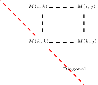
For convenience, the triple are called corners of the same rectangle (see Figure 1).
The three-point condition111The name is due to its resemblance to the four-point condition in the theory of -hyperbolic metric space (cf. remark after Proposition 6.13 of [24]). In our case, the base is fixed, therefore we only have to concern about the three remaining points. requires that must occur at least twice among , i.e., the two smallest values among the three must be equal.
Theorem 1.
An symmetric matrix is the Gromov matrix of a weighted tree if and only if the following conditions hold for :
-
(a)
has non-negative entries and all the diagonal entries of are positive.
-
(b)
For all , .
-
(c)
satisfies the three-point condition.
Proof:
Suppose that is a Gromov matrix with base . It is easy to show that conditions a and b hold from Definition 2. To verify condition c, suppose that correspond to the distinct indices of the matrix . The branch point is defined as the unique vertex of such that . The branch points and are defined similarly. If , then . Hence, we must have and . The case is similar. If , then . Hence A similar argument holds for the two inequalities and .
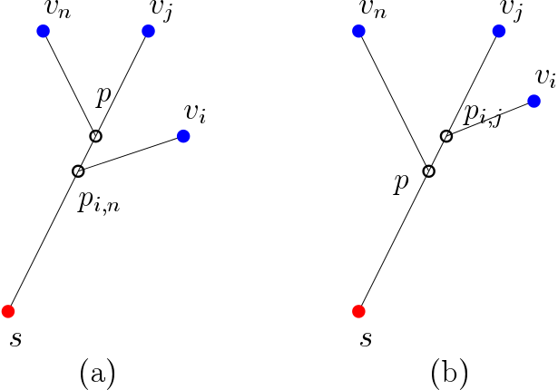
We prove the converse by induction on . The case are clearly true. Suppose the converse holds for all symmetric matrices satisfying the conditions a – c and for all . Consider a symmetric matrix satisfying conditions a – c. By the induction hypothesis, we can construct a base associated with the top-left matrix of . We add an additional node to as follows: Let be the index such that with corresponding vertex . Let be the vertex on the path such that ; and if it does not exist, we just let introduce it as a new vertex. We add an edge of weight to at and set and The tree is a well-defined weighted tree due to condition b. Furthermore, by construction.
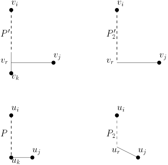
To see that is a base of , consider any index such that with corresponding vertex . From the induction hypothesis, it suffices to show that in . We consider two cases below (see Fig. 2 for illustrations).
Suppose that . Then, from the three-point condition c, we have . By our construction of , the branch point is on the path . This implies that , where the penultimate equality is due to the induction hypothesis.
On the other hand, if , then from the three-point condition c, we have . Therefore, in our construction of , we have and , where the penultimate equality is due to our construction. The converse is now proved, and so is the theorem. ∎
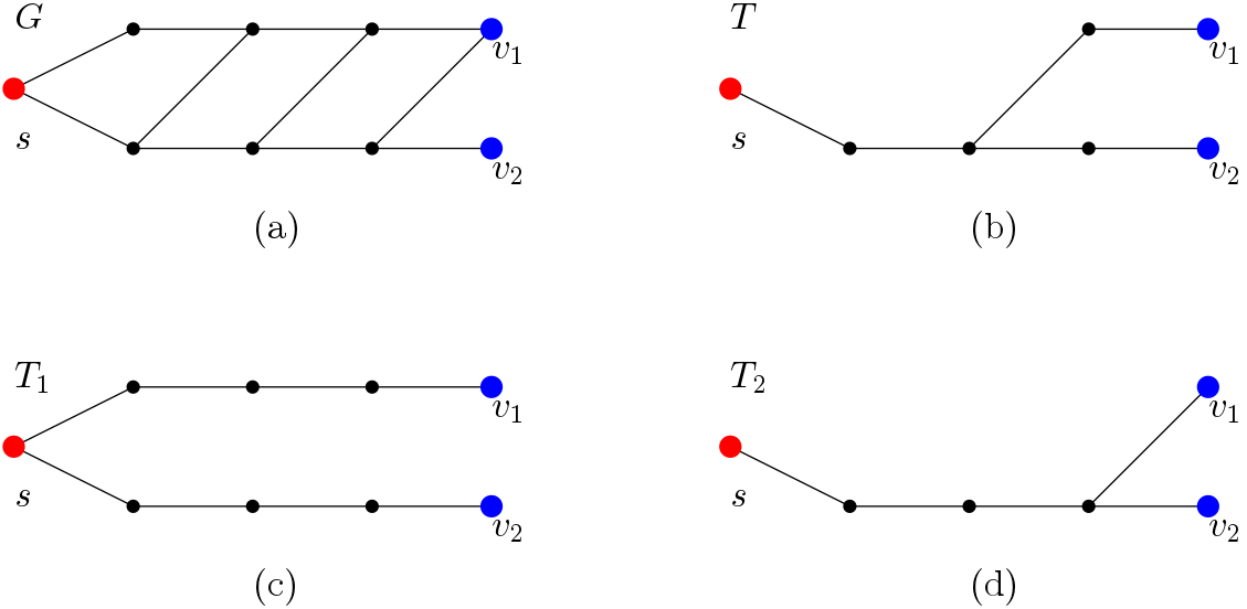
We have the following immediate corollary regarding convex combinations of special Gromov matrices (see Fig. 3 for an example).
Corollary 1.
Suppose that and are Gromov matrices of weighted trees and is diagonal. Then for any , the convex combination is the Gromov matrix of a weighted tree.
Proof:
It is easy to verify that satisfies the three conditions of Theorem 1. ∎
The conclusion does not hold in general if both and are not diagonal. In Section IV we describe a procedure to modify the convex combination of multiple Gromov matrices to a Gromov matrix.
We end this section by describing a few simple special examples to illustrate some basic properties of the Gromov product.
Example 2.
Let be a fixed base vertex of the tree and are two distinct nodes of .
-
(a)
If the Gromov product is , then is on the unique path connecting and . Therefore, if is a diagonal matrix, then is a star centered at .
-
(b)
The Gromov products if and only if is on the unique path connecting and .
-
(c)
The span of is either a line or star with leaves. The latter case happens if and only if
III Iterative Construction of a Gromov Matrix and Some Spectral Properties
In this section, we show positive definiteness of the Gromov matrix of a weighted tree as a byproduct of finding a lower bound of its least singular value, i.e., the smallest eigenvalue of . To do so, we describe an iterative way to construct from the empty matrix (of size ); and each step in the algebraic construction has a corresponding geometric counterpart, revealing additional geometric properties of . We delegate some long technical proofs to the appendices.
For two square matrices and of sizes and respectively, we introduce the following operations, called the Gromovication operations for convenience:
-
(a)
Initialization: for , replace the empty matrix by the -matrix .
-
(b)
Direct sum: is the square matrix with and forming the diagonal blocks; and elsewhere.
-
(c)
Extension I (of ): for an integer , is the matrix obtained from by adding to each entry.
-
(d)
Extension II (of ): for two positive integers such that , is the matrix obtained from by adding to each entry of , followed by increasing the number of rows and columns of each by one, and setting as the entries of the -th row and column.
Proposition 1.
is the Gromov matrix of a weighted tree with vertex set if and only if for some permutation matrix , can be obtained from the empty matrix by a finite sequence of Gromovication operations, starting with an initialization step.
Proof:
See Appendix A. ∎
Suppose that is a Gromov matrix. We study the its least singular value, which is defined as , the minimal eigenvalue of . As a corollary, we prove that is always positive definite.
Proposition 2.
Let and be Gromov matrices. We have the following results regarding the Gromovication operations.
-
(a)
Direct sum:
-
(b)
Extension I: For any positive integer ,
-
(c)
Extension II: For any integers ,
-
(a)
If ,
-
(b)
If ,
where is the number of rows of .
-
(a)
Proof:
See Appendix B. ∎
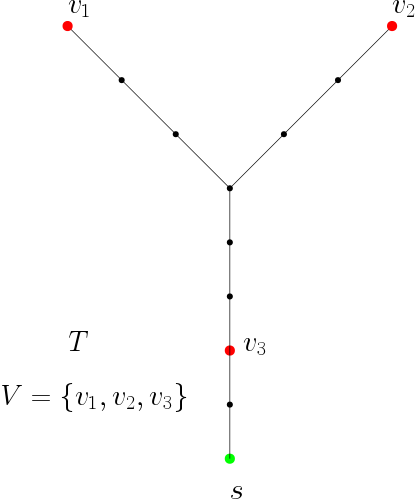
Proposition 2 can be useful in computation as shown in the example given in Fig. 4. Another immediate consequence is the following result.
Corollary 2.
Suppose that is a Gromov matrix with base . If is non-empty, then is positive definite.
Proof:
From Proposition 1, there exists a permutation matrix such that is formed by a finite sequence of Gromovication operations. Note that and have the same eigenvalues, thus it suffices to show that is positive definite. Since is non-empty, we start with an initialization, making the matrix positive definite. From Proposition 2, the matrix remains positive definite for any additional Gromovication operations, and the corollary is proven. ∎
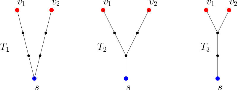
Intuitively, the least singular value of a Gromov matrix encodes geometric information of its base tree . If the least singular value of is small, the leaves of tend to be less branched off. We illustrate this intuition by a simple example in Fig. 5.
IV Convex Combinations of Gromov Matrices
In this section, we discuss two different ways to construct new matrices from existing Gromov matrices based on convex combination. We also compare the advantages of each approach. Through a case study, we provide further insights into how well convex combinations of Gromov matrices can approximate an information propagation path in a network.
IV-A Two Types of Convex Combinations
Suppose we are given a finite collection of Gromov matrices , all of the same dimensions. For each -tuple of numbers such that , define a new matrix as We call the convex combination of , for convenience.
To gain some geometric intuition, let be a Gromov matrix (such that the associated base is ) and be the diagonal matrix formed by the diagonal of . In , the off-diagonal entries of are being scaled down. Let be the joint point at the intersection of the paths and . Taking convex combination decreases , which means that geometrically, the joint point is being re-positioned along both the paths and . Therefore, the convex combination can be used as a tool that re-scales the edge weights of a tree.
In general, the convex combination is not always a Gromov matrix of any weighted tree, as the three-point condition is not preserved under matrix addition. There are various ways to modify the entries of to obtain a Gromov matrix. We provide one such procedure here, which turns out to be very natural. Consider the base case where and without loss of generality, we assume that . To ensure the three-point condition and minimum changes to the ordering, we essentially have 2 options: (1) replace by ; or (2) replace by . For each option, we only need to make one change in the top-right part of . For these two options, one increases the entries of while the other decreases the entries. As we can scale down the matrix entries by taking convex combination with a diagonal matrix, our preferred choice is to increase the entries in this procedure using option (1). We then apply option (1) whenever we encounter triples violating the three-point condition. A systematic way to do this is described in the following.
First set . Let denote the sequence of entries with (i.e., the upper-triangular block excluding the diagonal) in non-increasing order with . If corresponds to , then is called the matrix indices of . For each in increasing order, we perform the following steps:
-
(a)
Search for every pair satisfying the following two conditions:
-
•
; and
-
•
are corners of the same rectangle (Definition 2).
-
•
-
(b)
If the matrix indices of is , we perform the following two steps:
-
•
Set and .
-
•
Move to be immediately after in .
In doing so, the matrix indices of becomes and the sequence remains non-increasing.
-
•
Once the above procedure is completed, we symmetrize by assigning for all . We call a Gromovied convex (G-convex) combination of w.r.t. . Note that for each , there are at most pairs satisfying condition (a). The computational complexity of forming is . Therefore, the complexity of forming a G-convex combination is .
As we are enforcing the three-point condition each time we make an adjustment, the matrix is the Gromov matrix of a weighted tree by Theorem 1. The matrix has the property that for any Moreover, if is already a Gromov matrix, then is the same as
Throughout the rest of this paper, when we talk about the convex or G-convex combination of a set of Gromov matrices , we assume for convenience that every Gromov matrix in has the same base vertex and base set.
Let be a general graph, be a fixed set of distinct vertices of and a fixed node. In general, the spanning trees of rooted at are not unique and it is intractable to find all of them. However, if we are able to find a finite subset of spanning trees, we are able to use the G-convex combination construction to form a large family of trees . Doing so, we obtain a much larger candidate set than a randomly selected spanning tree, partially overcoming the intractability problem mentioned above. This can be useful in dealing with certain inference and estimation problems on graphs (see Section V). Note however that although each G-convex combination has a corresponding tree, this tree need not be a subgraph of . On the other hand, we hope that captures some distinctive structural features of in . We provide one such feature as follows.
Definition 3.
Let be a tree in a graph spanning a subset of distinct vertices and a fixed base vertex . The type of in is a partition of such that and (where is a permutation of the indices ) and .
Some thought will convince the reader that Definition 3 is non-vacuous and the type of any set of three distinct vertices exists. Furthermore, the type of is not unique if and only if . Intuitively, the notion of type describes the relative positions of nodes in a tree w.r.t. a fixed base node. We provide Example 3 below to illustrate this notion. Before that, we first prove an elementary result.
Suppose we form the convex combination , where and , of two Gromov matrices and , with being a diagonal matrix. Let the trees corresponding to , and be , and , respectively. For any , its type in is the same as its type in This observation is not true in general if is not diagonal. Instead, we have the following weaker statement regarding the convex combination of an arbitrary finite set of Gromov matrices and type.
Proposition 3.
Let be a finite set of Gromov matrices with corresponding base trees with the common base vertex and base set . Consider a subset of distinct vertices. For any convex combination weight vector , let and be the convex and G-convex combination of , respectively. Suppose is the tree corresponding to . For any triplet if
| (2) |
then a type of in is the same as its type in one of .
Proof:
From (2), we can take as a type in . As and each entry of is at least as large as the corresponding entry of , we have and .
Suppose that no type of in is the same as its type in any of , i.e., for each , is not a type in . Therefore in , we have either or from the three-point condition. Taking convex combination, we have either or This gives a contradiction. ∎
Proposition 3 places restrictions on , the tree corresponding to a G-convex combination . In particular, certain triplet node types must come from one of the components forming the G-convex combination, which corresponds to a spanning tree in the graph. Heuristically, taking G-convex combinations has two basic effects: (1) re-scaling distance and (2) mixing up types of the spanning trees in the components forming the G-convex combination. We illustrate the concepts and ideas of this section by the following example.
Example 3.
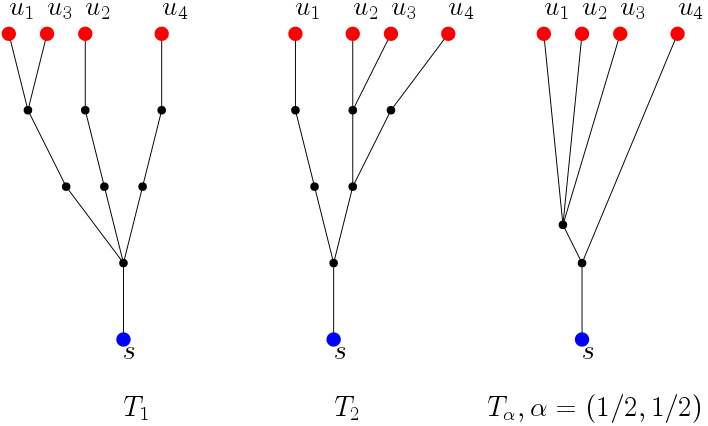
Consider Fig. 6. Let be the tree with Gromov matrix
and be the tree with Gromov matrix
both of which has base set . In , is of type , while in , is of type Hence are of different types in and . Let , with the convex combination of and given by
which is not a Gromov matrix. On the other hand, the G-convex combination matrix is
The tree is shown in Fig. 6. In , is of type , the same as its type in .
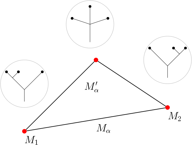
The set of symmetric matrices of fixed size is a vector space. Given two fixed Gromov matrices of the same size , for varying from to , the convex combinations , where , give a linear path from to in the convex cone of positive definite symmetric matrices of size . However, this linear path may not stay in the space of Gromov matrices. On the other hand, the family of G-convex combination matrices traces a continuous path between the end points and , as shown in the following theorem. A path is piecewise linear if it is continuous and is a finite union of line segments of the vector space.
Theorem 2.
The family of G-convex combinations of the Gromov matrices and traces a piecewise linear path from to . In particular, it is continuous in in the space of Gromov matrices.
Proof:
See Appendix C. ∎
In the following, we illustrate Theorem 2 using a toy example.
Example 4.
Consider two Gromov matrices
such that and . According to Definition 3, this is a case when their base sets are of different types (the other case is when the inequalities are reversed and the discussions are similar). For and , the convex combination of and is given by
It is clear that . The matrix is not a Gromov matrix. To construct the G-convex combination , we replace by It can be shown that if and only if
Therefore, for , we have
and for ,
We see that as increases from to , moves along a linear path first from to , and then from to . From the expressions of and , we see that they agree with each other only when . Therefore, the convex combinations of and for any are not Gromov. For a graphical illustration, see Fig. 7(a).
Since the path is piecewise linear in , we can define the turning points as those such that in a small neighborhood of which, the path fails to be linear. Inspired by the above example, we make the following observation.
Corollary 3.
Consider the family of G-convex combinations of the Gromov matrices and and suppose and are two successive turning points with corresponding base trees and . Then any triplet of distinct vertices in the base set has the same type in and .
Proof:
Suppose there exists a triplet that has different types in and . Then as discussed in Example 4, convex combinations of and are not Gromov matrices. Therefore, there must be other turning points between and , and it contradicts our assumption that and are successive turning points. ∎
The corollary suggests the following intuition: at each turning point, there is a transition of some types of triples, and it is the place where several branches merge together exactly.
To end this subsection, we make a comparison between the convex combination and G-convex combination , and discuss the advantages of each approach.
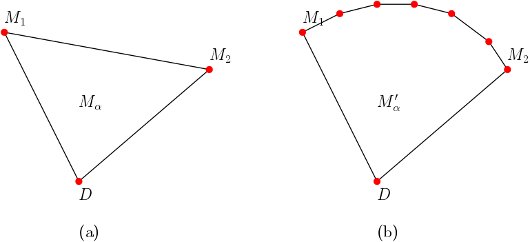
First, suppose we consider two general Gromov matrices and a diagonal one . We form both the convex combination and G-convex combination . According to Theorem 2, if we place them in the space of square matrices, they look like the bounded regions in Fig. 8. The shapes differ slightly, but are still quite similar. If we want to use either or to approximate another matrix of the same size, the result of the two approaches should be comparable.
Both convex and G-convex combinations have the following advantages in network inference and estimations:
-
(a)
Interpolation with uniform selections of allows us to select candidates uniformly in the space of symmetric matrices.
-
(b)
Even if the network topology is missing, estimations can still be performed if a few selected spanning trees are given.
Additional details are provided in Section V in conjunction with applications. Yet, due to differences in the constructions, each approach has its own advantages. The following trade-offs should be taken into consideration:
-
(a)
The computational cost of forming is lower than that for computing .
-
(b)
If the cost function varies smoothly w.r.t. the matrix entries, continuous optimization techniques (e.g., convex optimization) can be used to optimize over . This is more difficult for as it does not have an analytical form.
-
(c)
Spectral properties of are better understood, by tools such as the Weyl inequality.
-
(d)
The main disadvantage of the convex combination is that part of the geometric information is lost; and we are not able to recover any tree in general. On the other hand, for each , the G-convex combination gives a genuine Gromov matrix of a weighted tree. Therefore, the geometric content is preserved and we are able reconstruct the associated tree with ease (see Appendix D for a discussion.) The reconstruction process has complexity , where is the size of its base set. We point out here that itself may not be a subtree of . However, serves as a good approximation of a spanning tree.
IV-B A Case Study on Information Propagation Paths
We analyze and discuss a case study based on information propagation paths to illustrate how well G-convex combinations can approximate a tree of interest. For a graph and a source node , we generate propagation times on each edge in independently using a truncated Gaussian distribution. Let be a shortest path tree from , which can be interpreted as the information propagation path from . Let be the associated Gromov matrix.
We find a random BFS tree based at . Let be its Gromov matrix and be the norm of the difference between and . We choose another BFS tree based at with the associated matrix and let be the diagonal matrix of . Now we form G-convex combinations between and with parameter to obtain ; and then form G-convex combinations between with with parameter to obtain . Let . We have and we want to know how large is the ratio . A larger ratio means the Gromov method gives a better approximation of .
For the choice of and , we let their components be integer multiples of . As a consequence, we do not have to deal with too many G-convex combinations. On the other hand, the scale is fine enough such that the convex combinations (being uniformly distributed in the space of symmetric matrices) give reasonably good approximations to an actual spanning tree.
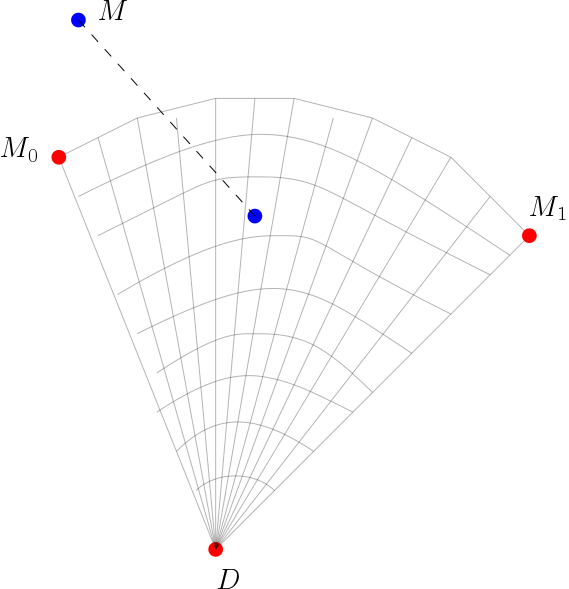
We perform simulations on both synthetic Erdös-Rényi (ER) graphs and the Enron email network222https://snap.stanford.edu/data/email-Enron.html (as an example of a scale-free graph) with nodes. For convenience, we fix the variance of the truncated Gaussian distribution as and vary the mean . Intuitively, if the mean is larger, the information propagation path looks more like a BFS tree. The simulation results are plotted in Fig. 9. We observe that if is larger (i.e., the actual information propagation path resembles a BFS tree more closely), then our approach gives a much better approximation of than simply choosing a random BFS tree . The intuition is as follows: even though the randomly chosen BFS trees are not close to , there exists a projection of in the convex region formed by , , and (see Fig. 10). This example suggests that by using G-convex combinations to approximate the information propagation path in problems where is unknown a priori is a better approach than the spanning tree heuristic.
V Applications of the Gromov Method
The theory developed in this paper can be used as an alternative to the spanning tree heuristic in network inference and estimation problems proposed by various works like [9, 10, 11, 12, 13, 25]. Suppose we are given a graph , a subset of nodes , and an estimator or cost function taking as inputs a tree spanning and base vertex , with satisfying certain criteria according to the problem of interest. We denote by the set of all satisfying these criteria. An inference problem typically involves computing
| (3) |
where the expectation is w.r.t. a distribution over , or
| (4) |
As the cardinality of is often very large, the spanning tree heuristic approximates the solution by randomly choosing a small subset and computing either or instead. For our Gromov method, instead of randomly selecting a spanning tree, we let be obtained by taking either convex or G-convex combinations of the trees in . For example, for every and with associated Gromov matrices and in , we can let be the diagonal matrix taking the diagonal of and form . We then form either a convex combination or G-convex combination from . All such combinations are then included in . We then compute or . It is clear that the Gromov method achieves a better approximation since , but requires higher computational complexity. We remark here that as a general suggestion, when we form G-convex combination, it usually suffices to choose each weight parameter as integer multiples of or in .
The advantages of the Gromov method are as follows:
-
(a)
Taking the convex or G-convex combination gives us a larger family of approximate spanning trees, while retaining certain structural features of the ambient graph (see Corollary 1, Fig. 3 and Proposition 3). Standard optimization techniques may then be applied to optimize over this family. For the convex combination approach, we may use continuous optimization tools. For -convex combinations, we perform a discrete optimization with fixed size increments on the combination weights.
-
(b)
In some applications, we may not have access to all the spanning trees satisfying the problem criteria, or it may be computationally complex or practically expensive to find such spanning trees. It becomes difficult to construct many spanning trees using the tree heuristic. With the Gromov method, we mitigate this problem by using only a small set of spanning trees and then forming convex or G-convex combinations from them.
In the following, we present several network inference applications to illustrate the use of the Gromov method.
V-A Information Acquisition Order
Suppose that information is propagated stochastically from a source node in a graph , where the propagation time distribution along each edge is known. An important application is knowing if on average a node lies on the propagation path from to another node . For example, in viral marketing and social learning (e.g., [26, 4, 6, 7]), we are interested to find those nodes in a social network that act as the gatekeepers of information propagation. In infection control and monitoring (e.g., [17, 27, 28, 29, 30]), we are interested to identify those nodes in a network with the highest probability of acquiring the infection and spreading it to others in the network so that we can add monitoring and countermeasures at these nodes.
Information propagation from follows a random spanning tree . Computing the probability that , where is the unique path in connecting and is intractable for a dense graph . Furthermore, such a computation requires full knowledge of the propagation statistics and graph topology. To estimate this probability empirically, we can sample a large number of random spanning trees containing and . For each such spanning tree , we decide if is on the unique path connecting and or not. We can then compute the empirical probability of instances of . This problem is of the form Problem (3), where is the indicator function of the event that .
In actual applications, we may not have the resources to sample so many random spanning trees. For example, in viral marketing, each sample involves an information dissemination campaign, which can be expensive to repeat. In the Gromov method, we may sample a very small number of spanning trees, and use G-convex combinations to synthesize more spanning trees.
It is interesting to note that to perform this estimation, we do not even need to know the network topology, provided we are given a few samples. This is a very useful feature for practical applications as inferring the full network topology is usually not an easy task. In this problem, we need to use G-convex combinations, as geometric information of the synthesized trees is used.
We performed simulations on four types of graphs: 2D-lattice, the Enron email network, a sample Facebook network333https://snap.stanford.edu/data/egonets-Facebook.html and the complete graph, as an extreme case. For each simulation trial, a random sample is generated as follows: (1) propagation timestamps across the network are simulated; (2) a minimum spanning tree is then chosen by Dijkstra’s algorithm. For the Gromov method, we sample three spanning trees and form G-convex combinations between each pair of sampled spanning trees by choosing in the combination weight vector uniformly from in integer multiples of , giving approximately synthesized trees. The ground truth is obtained by averaging over samples depending on the density of the network.
The accuracy of the Gromov method is then computed as follows: For each triple of nodes , from the ground truth, we may find the empirical probability of (1) , (2) as and . On the other hand, the Gromov method gives estimations and . The error is calculated as . The accuracy is obtained by averaging over different triples .
It is useful to notice that the size of the network is not a crucial factor here since we only need to make sure the spanning tree is large enough to contain the three involved nodes. On the other hand, the ratio between the average node degree and the number of nodes gives an important indication of the density of the graph. The simulation results are shown in Table I. We see that the Gromov method performs reasonably well and yields a good estimation with a limited number of samples.
| Degree-node ratio | Accuracy | |
|---|---|---|
| 2D-lattice | 0.04 | 95.1% |
| Email network | 0.094 | 95.3% |
| Facebook network | 0.268 | 91.1% |
| Complete graph | 1 | 94.0% |
V-B Network Source Identification
We consider the problem posed in Example 1 in the introduction. We start with the case where a snapshot of the infection status of each node is observed. We assume that infection propagation along each edge follows an exponential distribution with mean . Suppose we are given a snapshot of all the infected nodes. We want to estimate the identity of the source node. One possible approach is estimator based. An estimator is a real valued function on each candidate source node and a spanning tree of rooted at . The source is found by maximizing over all . In the spanning tree heuristic adopted by [9], for a general graph, a random BFS tree is usually chosen as the second argument of , which might be a source of error in the estimation.
Various estimators have been studied in the literature [9, 31, 18, 32], and for demonstration purposes, we choose the centroid as an example. The centroid (see [18]) is defined as the maximal size, i.e., the sum of all the edge weights, of connected components of . This problem is of the form Problem (4), where we seek to minimize the cost function over all trees rooted at that span the observed infected nodes . In the spanning tree heuristic, this optimization is done in the following way:
-
(a)
For each candidate source , we randomly choose a BFS tree .
-
(b)
The infection source is then estimated by .
In the Gromov method, for each base vertex , we first fix an ordering of the nodes. We choose the BFS tree (with its Gromov matrix) according to this ordering and the BFS tree with the reverse node ordering. Let be the tree associated with the diagonal matrix of , for edge weights scaling. We use as the initial spanning trees to form G-convex combinations by setting the combination weight vector so that each is an integer multiple of chosen uniformly in with . We then estimate the source by .
| Ave. Deg. | Size | Err. Red. | Detect. Improve. | |
|---|---|---|---|---|
| BA | 4 | 500 | 12.4% | 73.7% |
| ER | 4 | 500 | 18.6% | 25.8% |
| 9.86 | 670 | 12.7% | 25.0% | |
| 35.7 | 786 | 2.1% | 29.4% |
We run simulations on both synthetic and real networks: Barabási-Albert (BA) graphs with vertices and degree , ER graphs with vertices and average degree , the Enron email network with vertices and average degree , and the Facebook network with vertices and average degree . In each simulation, we infect to of the vertices where the infection propagation time from an infected node to an uninfected neighbor follows an exponential distribution with rate 1. Let the average distance between the true source and the estimated source be for the BFS heuristic and for the Gromov method. The error reduction rate shown in Table II is given by . We also compute the fraction of trials for which the source is among the top highest scoring nodes determined by each method (i.e., the -accuracy). Let this be for the BFS heuristic and for the Gromov method. We compute the detection improvement as in Table II. We see noticeable improvement when using the Gromov method in most of the cases. The error reduction for the Facebook network is smaller because the network is very dense. However, we see significant improvement in the -accuracy score.
(a) BA graph
(b) ER graph
(c) Email
(d) Facebook
(a) BA graph
(b) ER graph
(c) Email
(d) Facebook
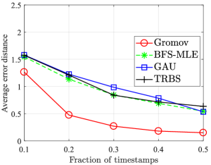
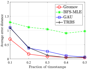
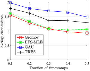
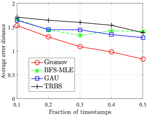
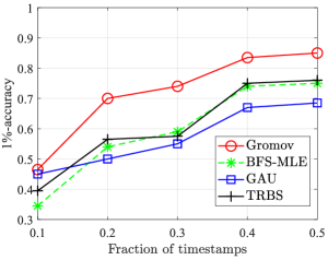
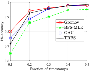
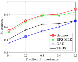
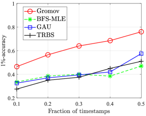
Another variant of the problem is source estimation with observed infection timestamps. Here, we assume that a small percentage of the infected nodes are observed, together with their respective infection timestamps. We apply the Gromov method (using convex combination), similar to the snapshot observation based estimation described above (we refer the reader to [21] for details). We compare the Gromov method with the BFS tree based approach (called BFS-MLE), as well as other approaches: GAU [10] and TRBS [33], on various networks. We use average error distance as well as -accuracy as the evaluation metrics. The results are shown in Fig. 11 and Fig. 12, which are reproduced from [21] here for completeness. We vary the number of nodes with observed timestamps. We observe significant performance improvement using the Gromov method in most cases.
V-C Data Center Placement
In this application, we consider the problem of determining the optimal placement of data centers in a large network [34, 35, 36, 37, 38, 39, 40]. The network is given by a weighted graph . For each node , a non-negative number is associated to it to indicate the service demand at . Given a subset and , let i.e., path length from to the node in closest to . The overall weighted cost of serving by is defined as . We want to find a subset , where is the number of data centers. This problem is similar to Problem (4), except that now we are finding an optimal subset of nodes.
An iterative greedy algorithm was proposed by [40] to solve this problem as follows: Let . In each iteration , suppose that a set of data centers with nodes has been found. Find the node and let . Note that the greedy algorithm may not find the optimal solution.
We propose a Gromov method based on the algorithm in [25], which we enhance using the Gromov techniques discussed in this paper. The steps are as follows:
-
(a)
Randomly choose an initial set of nodes .
-
(b)
For each iteration , partition using a Voronoi partition with vertices from as the centers. For each Voronoi partition or subgraph , find a minimum spanning tree and a BFS tree rooted at its center . Let be the set of trees formed by the G-convex combination of these two spanning trees, where we choose the combination weight vector so that each is an integer multiple of chosen uniformly in . Solve for (using Algorithm 2 in [25]) to find . Set .
-
(c)
Iterate till for some small .
Intuitively, the Gromov method attempts to evenly distribute the data centers across the network. Therefore, a improvement over the greedy approach is possible, as the latter may result in some data centers being ineffectively placed.
We run simulations on both grid networks and CAIDA AS graphs (see [41]). We vary both the graph size ( to nodes) and number of data centers ( of the total number of nodes) for each graph type. The service demand for each node is generated according to the Pareto distribution, which is a power-law distribution used to model the situation where a small number of nodes generate most of the service demand.
For each instance, we compute the estimated cost for the greedy method, and for the Gromov method. The performance of the two methods are compared by taking the average of the ratio . The simulation results are shown in Fig. 13. We see that the Gromov method has a better performance in almost all the cases (average cost ratio ).
VI Conclusion
In this paper, using the Gromov matrix interpretation of trees, we have proposed a modified version of the commonly used spanning tree heuristic, which we call the Gromov method, in network inference problems. We presented both necessary and sufficient conditions for a matrix to be a Gromov matrix of a weighted tree, followed by a demonstration on how to form convex combination of Gromov matrices. The Gromov method proposed is based on optimizing the network inference objective function over a parametrized family of Gromov matrices. We give some applications of the Gromov method on network inference and estimation. As the proposed Gromov method provides a general framework, it is of interest to explore other network inference and estimation applications in future works. Moreover, how to choose the appropriate matrices or spanning trees in forming the convex combinations is also an interesting and important topic to explore.
Appendix A Proof of Proposition 1
Suppose that the base of is . We first note that conjugation by permutation matrices is equivalent to a re-ordering of the indices of . Therefore, we can ignore the ordering of the indices in our proof. To prove the proposition, it suffices to prove that the weighted tree with base can be obtained from the Gromovication operations starting from .
We first observe that each Gromovication operation on Gromov matrices corresponds to the construction of a new base from the bases associated with the input Gromov matrices as follows (see Fig. 14 for an illustration).
-
•
Initialization: Given the base and , we form a tree by attaching an edge of weight to . Denote the other end of by and let . Then the base of the initialization is .
-
•
Direct sum: Given the bases and corresponding to the Gromov matrices and respectively, we form a new tree by joining the two trees and at their base vertices and identifying both and as a single base vertex . A base of is then .
-
•
Extension I (with parameter ): Given a base corresponding to the Gromov matrix , we form a new tree by attaching a path of length at , and letting be the other endpoint of . Then is a base of .
-
•
Extension II (with parameters ): Given a base corresponding to the Gromov matrix , we form a new tree by attaching a path of length at as in extension I, with being the other endpoint of . The path is constructed to have a vertex whose distance to is (it is possible that ). Then, the base corresponds to .
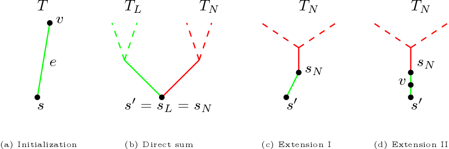
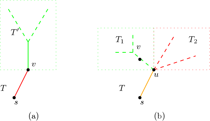
We now proceed to prove Proposition 1 for the base by induction on . As we assume that is non-empty, is non-empty. The case requires an initialization step. Suppose that the proposition is true when the base set has less than vertices. Let be a node such that There are two cases to consider (see Fig. 15 for an illustration):
-
(a)
The path does not contain any vertex of degree greater than . Let , and . As , by the induction hypothesis, we can obtain by the Gromovication operations. Moreover, can be constructed from by an extension II.
-
(b)
The path contains of a vertex of degree greater than . By our choice of , the node . We can always find two connected subtrees and of such that:
-
(i)
;
-
(ii)
;
-
(iii)
, for .
Let ; and , for The induction hypothesis implies that both can be obtained from Gromovication operations. Moreover, can be obtained from , by a direct sum followed by possibly an extension I.
-
(i)
The proof is now complete.
Appendix B Proof of Proposition 2
-
(a)
This is obvious.
-
(b)
Recall that a special case of Weyl’s inequality (cf.[42]) asserts the following: For two symmetric matrices and of the same size, the inequality
(5) holds. In view of Weyl’s inequality, it suffices to note that the matrix with identical entries has two eigenvalues and .
-
(c)
Let be the square matrix with all entries . If , we form two matrices: ; and has the block as its top-left submatrix, in the bottom-right corner, and the remaining entries . The column rank of is and it is easy to check that Moreover, from item a, . Therefore, as , we have the desired inequality
by Weyl’s inequality 5.
Suppose . Let . We form two matrices: ; and , which has in the bottom-right corner and everywhere else. As , by Lemma B.1 below and Weyl’s inequality, we have
The proof of the proposition is now complete.
Lemma B.1.
Suppose that is the matrix whose bottom-right corner is for some , and has everywhere else. Then
Proof:
It is enough to show that the characteristic polynomial of is We give a sketch of the proof with some calculation details omitted. First we note that has identical columns, the characteristic polynomial takes the form , where the coefficient is the trace .
Let , where is the identity matrix. To determine , let be the -th cofactor of ; and the -th entry of . The determinant The summand can be computed by induction as
For the remaining summands, only the leading coefficient of contributes to , which is either or ; and the coefficient of of is . It is now easy to obtain that ∎
Appendix C Proof of Theorem 2
We first prove an elementary lemma.
Lemma C.1.
For a triplet of real numbers , the new triplet defined by satisfies the following properties:
-
(a)
-
(b)
-
(c)
The triplet satisfies the three-point condition.
Proof:
Without loss of generality, we assume that . It is easy to verify that and Therefore, the lemma follows. ∎
For convenience, we call the max-min of w.r.t. . Suppose we have a pair of functions and . If both of them are piecewise linear continuous in , then so are and . Similarly, suppose we have functions such that all of them are piecewise linear continuous in . Then the same holds for the max-min of , w.r.t. .
We now proceed with the proof of Theorem 2. We have the following alternative (though inefficient) way of obtaining from the convex combination . The matrices constructed below depends on , but for convenience, we suppress in the notations. We start with and is obtained from as follows: given and , we first form the triple . Next, we find as the max-min of w.r.t. . The -th entry of is taken as . During this process, the only functions involved are and . Therefore, if the entries of are piecewise linear in the parameter , so are the entries of . Hence itself is piecewise linear in when considered as an element of the vector space of square matrices.
To conclude the proof of the theorem, we need to show two additional assertions:
-
(i)
The sequence of matrices stabilizes (the entries do not change in the next iteration) after a fixed number of iterations.
-
(ii)
The stabilized matrix is .
For i, we make the following observation: the largest off-diagonal entries of do not change in subsequent iterations. Denote by the positions of the entries of that do not change in all subsequent iterations, which is non-empty by the case . On the other hand, the largest off-diagonal entries of with positions different from do not change in all subsequent iterations. Therefore unless . Therefore the sequence of matrices stabilizes within iterations.
Appendix D Some Geometric Constructions
Suppose is a Gromov matrix with base , where . For each vertex pair , the distance between them can be recovered as The nodes in uniquely determine as span . However, we are not able to recover the (weighted) adjacency matrix of directly using such information, as may not contain all the vertices of in the usual sense (for a simple example, see Fig. 6). On the other hand, in certain applications, we are interested in the relative positions of vertices of on , instead of the relative distance (e.g., some applications may require only knowledge of the number of neighbors of certain vertices, or the size of the connected components after removing a particular node). In this appendix, we discuss certain geometric constructions based on , or equivalently , which allows us to explore the relative positions of the vertices of .
We first introduce a graph as follows: the size of is and let be the vertex set of . Two vertices and are connected by an edge in if and only if in . The weight of each edge of is set to be , and the distance metric on is denoted by .
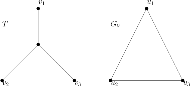
For each path (not required to be simple) in , we form an associated path in as follows: if is obtained from concatenating edges , we construct by concatenating simple paths . If with length is a path connecting and such that , then we call a geodesic path for convenience. One should take note here that is not a tree in general (cf. Fig. 16), and there can be multiple geodesic paths between two nodes.
Lemma D.1.
If is a geodesic path connecting and , then the associated path in is simple.
Proof:
Let the length of be . We prove the claim by induction on . The case clearly holds by definition.
Suppose the claim holds for . Consider . Let be the subpath of starting from of length . By the induction hypothesis, the associated path in is simple, connecting and . If the intersection in , then as the concatenation of and is simple; and this proves the lemma.
Otherwise, (see Fig. 17 for an illustration). In this case, there exists a in and . We can form another path consisting of concatenated with in . The path is of length strictly smaller than ; and hence . This contradicts the assumption that is a geodesic path. ∎
Since may not be a tree (cf. Fig. 16), and we have the following weaker substitute.
Corollary D.1.
For each , there is a unique BFS tree of based at .
Proof:
Suppose on the contrary that for there are two distinct BFS trees and of . This means that there is a vertex such that the following holds:
-
(a)
The path in and are distinct; and denote them by and respectively.
-
(b)
and are of the same length .
Let and be their associated paths (connecting say and ) in respectively. As and are distinct, so are and . Moreover, by Lemma D.1, both and are simple paths. This is absurd, as is a tree and there is a unique simple path connecting and . This concludes the proof of the corollary by contradiction. ∎
From this result, we see that resembles a tree in the sense that each node has a unique BFS tree. It is an important feature to handle information propagation. On the other hand, contains all the nodes of . Therefore, we may use to study the relative positions of nodes in of , as well as other combinatorial properties.
Now we indicate how to obtain the adjacency matrix of from the Gromov matrix . To determine the -th entry of , consider and in . As we have demonstrated, the distance can be recovered from . Moreover, recall that is a tree. Therefore if and only if for each , ; or equivalently,
Reconstructing thus requires a complexity of .
References
- [1] A. Guille, H. Hacid, C. Favre, and D. A. Zighed, “Information diffusion in online social networks: A survey,” SIGMOD Rec., vol. 42, no. 2, pp. 17–28, Jul. 2013.
- [2] D. Kempe, J. Kleinberg, and E. Tardos, “Maximizing the spread of influence through a social network,” in Proc. ACM SIGKDD Int. Conf. Knowledge Discovery and Data Mining, 2003, pp. 137–146.
- [3] A. Java, P. Kolari, T. Finin, and T. Oates, “Modeling the spread of influence on the blogosphere,” in Proc. Int. Conf. World Wide Web, 2006, pp. 22–26.
- [4] J. Leskovec, L. A. Adamic, and B. A. Huberman, “The dynamics of viral marketing,” ACM Trans. Web, vol. 1, no. 5, pp. 1–39, 2007.
- [5] W. P. Tay, “The value of feedback in decentralized detection,” IEEE Trans. Inf. Theory, vol. 58, no. 12, pp. 7226 – 7239, Dec. 2012.
- [6] D. W. Soh, W. P. Tay, and T. Q. S. Quek, “Randomized information dissemination in dynamic environments,” IEEE/ACM Trans. Netw., vol. 21, no. 3, pp. 681 – 691, Jun. 2013.
- [7] W. P. Tay, “Whose opinion to follow in multihypothesis social learning? A large deviations perspective,” IEEE J. Sel. Topics Signal Process., vol. 9, no. 2, pp. 344 – 359, Mar. 2015.
- [8] J. Ho, W. P. Tay, T. Q. S. Quek, and E. K. P. Chong, “Robust decentralized detection and social learning in tandem networks,” IEEE Trans. Signal Process., vol. 63, no. 19, pp. 5019 – 5032, Oct. 2015.
- [9] D. Shah and T. Zaman, “Rumors in a network: Who’s the culprit?” IEEE Trans. Inf. Theory, vol. 57, no. 8, pp. 5163–5181, 2011.
- [10] P. C. Pinto, P. Thiran, and M. Vetterli, “Locating the source of diffusion in large-scale networks,” Phys. Rev. Lett., vol. 109, p. 068702, 2012.
- [11] K. Zhu and L. Ying, “Information source detection in the SIR model: a sample path based approach,” in Proc. Information Theory and Applications Workshop, 2013.
- [12] W. Luo, W. P. Tay, and M. Leng, “How to identify an infection source with limited observations,” IEEE J. Sel. Topics Signal Process., vol. 8, no. 4, pp. 586–597, 2014.
- [13] F. Ji, W. P. Tay, and L. R. Varshney, “An algorithmic framework for estimating rumor sources with different start times,” IEEE Trans. Signal Process., vol. 65, no. 10, pp. 2517–2530, 2017.
- [14] W. Dong, W. Zhang, and C. W. Tan, “Rooting out the rumor culprit from suspects,” in Proc. IEEE Int. Symp. Inf. Theory, July 2013, pp. 2671–2675.
- [15] W. Luo and W. P. Tay, “Finding an infection source under the SIS model,” in Proc. IEEE Int. Conf. Acoustics, Speech, and Signal Process., May 2013, pp. 2930–2934.
- [16] A. Y. Lokhov, M. Mézard, H. Ohta, and L. Zdeborová, “Inferring the origin of an epidemic with a dynamic message-passing algorithm,” Phys. Rev. E, vol. 90, p. 012801, Jul 2014.
- [17] W. Luo, W. P. Tay, and M. Leng, “Rumor spreading and source identification: A hide and seek game,” IEEE Trans. Signal Process., vol. 64, no. 16, pp. 4228–4243, 2016.
- [18] C. W. Tan, P. D. Yu, C. K. Lai, W. Y. Zhang, and H. L. Fu, “Optimal detection of influential spreaders in online social networks,” in Proc. Annu. Conf. Inf. Sci. Syst., Mar. 2016, pp. 145–150.
- [19] A. Louni and K. P. Subbalakshmi, “A two-stage algorithm to estimate the source of information diffusion in social media networks,” in Proc. IEEE Conf. Comput. Commun. Workshops, April 2014, pp. 329–333.
- [20] W. Tang and W. P. Tay, “A particle filter for sequential infection source estimation,” in Proc. IEEE Int. Conf. Acoustics, Speech and Signal Process., Mar. 2017.
- [21] W. Tang, F. Ji, and W. P. Tay, “Estimating infection sources in networks using partial timestamps,” IEEE Trans. Inf. Forensics Security, vol. 13, no. 2, pp. 3035 – 3049, Dec. 2018.
- [22] F. Ji, W. Tang, and W. P. Tay, “Properties and applications of Gromov matrices in network inference,” in Proc. IEEE Workshop on Statistical Signal Processing, Jun. 2018.
- [23] I. Kapovich and N. Benakli, “Boundaries of hyperbolic groups,” arXiv preprint math/0202286, 2002.
- [24] B. Bowditch. (2006) A course on geometric group theory. [Online]. Available: http://homepages.warwick.ac.uk/~masgak/papers/bhb-ggtcourse.pdf
- [25] W. Luo, W. P. Tay, P. Sun, and Y. Wen, “On distributed algorithms for cost-efficient data center placement in cloud computing,” arXiv preprint abs/1802.01289, 2018.
- [26] P. Domingos, “Mining social networks for viral marketing,” IEEE Intelligent Systems, vol. 20, no. 1, pp. 80–82, 2005.
- [27] R. Pastor-Satorras and A. Vespignani, “Epidemic spreading in scale-free networks,” Phys. Rev. Lett., vol. 86, pp. 3200–3203, 2001.
- [28] Z. Dezső and A.-L. Barabási, “Halting viruses in scale-free networks,” Phys. Rev. E, vol. 65, p. 055103, 2002.
- [29] R. Pastor-Satorras and A. Vespignani, “Immunization of complex networks,” Phys. Rev. E, vol. 65, p. 036104, 2002.
- [30] Y. Wang, G. Xiao, J. Hu, H. Tee, T. Cheng, and L. Wang, “Imperfect targeted immunization in scale-free networks,” Physica A: Statistical Mechanics and its Applications, vol. 388, no. 12, pp. 2535 – 2546, 2009.
- [31] W. Luo, W. P. Tay, and M. Leng, “On the universality of Jordan centers for estimating infection sources in tree networks,” IEEE Trans. Inf. Theory, vol. 63, no. 7, pp. 4634 – 4657, Jul. 2017.
- [32] K. Zhu and L. Ying, “Information source detection in the SIR model: A sample-path-based approach,” IEEE/ACM Trans. Netw., vol. 24, no. 1, pp. 408–421, Feb. 2016.
- [33] Z. Shen, S. Cao, W. Wang, Z. Di, and H. E. Stanley, “Locating the source of diffusion in complex networks by time-reversal backward spreading,” Phys. Rev. E, vol. 93, p. 032301, Mar 2016.
- [34] B. Li, M. J. Golin, G. F. Italiano, X. Deng, and K. Sohraby, “On the optimal placement of web proxies in the internet,” in Proc. IEEE INFOCOM 1999, 1999.
- [35] K. Jain and V. V. Vazirani, “Approximation algorithms for metric facility location and k-median problems using the primal-dual schema and lagrangian relaxation,” Journal of the ACM, 2001.
- [36] M. Charikar, S. Guha, Éva Tardos, and D. B. Shmoys, “A constant-factor approximation algorithm for the k-median problem,” Journal of Computer and System Sciences, 2002.
- [37] V. Arya, N. Garg, R. Khandekar, A. Meyerson, K. Munagala, and V. Pandit, “Local search heuristics for k-median and facility location problems,” SIAM Journal on Computing, 2004.
- [38] N. Laoutaris, G. Smaragdakis, K. Oikonomou, I. Stavrakakis, and A. Bestavros, “Distributed placement of service facilities in large-scale networks,” in Proc. IEEE INFOCOM 2007, 2007.
- [39] K. Oikonomou, G. Tsioutsiouliklis, and S. Aissa, “Scalable facility placement for communication cost reduction in wireless networks,” in IEEE ICC 2012 - Wireless Networks Symposium, 2012.
- [40] L. Qiu, V. N. Padmanabhan, and G. M. Voelker, “On the placement of web server replicas,” in Proc. IEEE INFOCOM, 2001, pp. 1587–1596.
- [41] J. Leskovec, J. Kleinberg, and C. Faloutsos, “Graphs over time: Densification laws, shrinking diameters and possible explanations,” in Proc. ACM SIGKDD Int. Conf. Knowledge Discovery and Data Mining, 2005, pp. 177–187.
- [42] J. Franklin, Matrix Theory. Dover Publications, 1993.