Evolution of the Star-Forming Galaxies from $z=0.7$ to 1.2 with eBOSS Emission-line Galaxies

Abstract

We study the evolution of star-forming galaxies with $10^{10}M_{\sun}<M_{*}<10^{11.6}M_{\sun}$ over the redshift range of $0.7<z<1.2$ using the emission-line galaxies (ELGs) in the extended Baryon Oscillation Spectroscopic Survey (eBOSS). By applying the incomplete conditional stellar mass function (ICSMF) model proposed in Guo et al. (2018), we simultaneously constrain the sample completeness, the stellar–halo mass relation (SHMR) and the quenched galaxy fraction. We obtain the intrinsic stellar mass functions for star-forming galaxies in the redshift bins of $0.7<z<0.8$, $0.8<z<0.9$, $0.9<z<1.0$ and $1.0<z<1.2$, as well as the stellar mass function for all galaxies in the redshift bin of $0.7<z<0.8$. We find that the eBOSS ELG sample only selects about 1%–10% of the star-forming galaxy population at the different redshifts, with the lower redshift samples to be more complete. There is only weak evolution in the SHMR of the ELGs from $z=1.2$ to $z=0.7$, as well as the intrinsic galaxy stellar mass functions. Our best-fitting models show that the central ELGs at these redshifts live in halos of mass $M\sim 10^{12}M_{\sun}$, while the satellite ELGs occupy slightly more massive halos of $M\sim 10^{12.6}M_{\sun}$. The average satellite fraction of the observed ELGs varies from 13% to 17%, with the galaxy bias increasing from 1.1 to 1.4 from $z=0.7$ to 1.2.

1. Introduction

The next-generation large-scale galaxy redshift surveys will probe much larger volumes into the deeper universe than the existing surveys, e.g., the 2dF Galaxy Redshift Survey (2dFGRS; Colless, 1999) and the Sloan Digital Sky Survey (SDSS; York et al., 2000; Gunn et al., 2006). Efficient tracers of the large-scale structure are necessary to probe the high-redshift universe. For example, the Dark Energy Spectroscopic Instrument (DESI; DESI Collaboration et al., 2016) is targeting the luminous red galaxies (LRGs) up to $z=1.0$ and the star-forming galaxies with strong nebular emission lines, a.k.a. emission-line galaxies (ELGs), up to $z=1.7$. The Prime Focus Spectrograph (PFS; Takada et al., 2014) will target ELGs over a wide redshift range of $0.8<z<2.4$ to constrain the cosmological parameters and study the galaxy evolution. The 4-meter Multi-Object Spectroscopic Telescope (4MOST; de Jong et al., 2016) also treats the ELGs as main targets for cosmological probes at redshifts $0.7<z<1.2$. The Hobby-Eberly Telescope Dark Energy Experiment (HETDEX; Hill et al., 2008) will target more than a million [O II] emitting ELGs at $z<0.5$.

The [O II] doublet emitters are of particular interest to these high-redshift ELG surveys, as their strong emission lines at the rest-frame wavelengths of $3727$ and $3729\leavevmode\nobreak\ \rm{\AA}$ will make it easier to accurately measure redshifts beyond $z=1$, where the LRGs are no longer efficient cosmological tracers (Zhu et al., 2015). These [O II] emitters are also important tracers of the cosmic star formation history (Kewley et al., 2004; Orsi et al., 2014), as the cosmic star formation rate (SFR) peaks around $z\sim 2$ (see, e.g., Behroozi et al., 2013a; Yang et al., 2013). In addition, the broad stellar mass range probed by these ELGs makes them good tracers of the galaxy stellar mass function (SMF), especially the region around the knee of the SMF (Comparat et al., 2017b).

Some of the physical and clustering properties of the ELGs have been investigated in previous studies. For example, by combining the ELG galaxy samples in the VIMOS VLT Deep Survey (VVDS; Le Fèvre et al., 2013) and the DEEP2 survey (Newman et al., 2013), Comparat et al. (2016b) found that the characteristic luminosity of the [O II] luminosity function increases by a factor of 2.7 from $z=0.5$ to 1.3. Favole et al. (2016) constructed a sample of g-band-selected galaxies from the Canada-France-Hawaii Telescope Legacy Survey (CFHT-LS; Ilbert et al., 2006), which is expected to be dominated by ELGs in the redshift range of $0.6<z<1$. They found that the typical host halo mass of ELGs at $z\sim 0.8$ is around $10^{12}h^{-1}M_{\sun}$ (see also Orsi et al., 2014; Gonzalez-Perez et al., 2018) and the satellite fraction of the selected sample is about 22.5%.

The number of observed high-redshift star-forming galaxies with emission line measurements is growing quickly with recent optical and near-infrared surveys (see e.g., Comparat et al., 2016a; Okada et al., 2016; Delubac et al., 2017; Kaasinen et al., 2017; Drinkwater et al., 2018). But the sample sizes of the current ELG surveys are still not large enough to fully understand the properties of the high-redshift ELGs. The SDSS-IV extended Baryon Oscillation Spectroscopic Survey (eBOSS; Dawson et al., 2016) has recently finished its ELG survey program, and the final sample consists of about 0.2 million [O II] ELGs covering the redshift range of $0.6<z<1.2$. Although the [O II] emitters in eBOSS are mainly used as the cosmological tracers (Zhao et al., 2016) and the galaxy spectra are quite noisy, the large ELG sample provides an opportunity to better understand the evolution of star-forming galaxies since $z=1.2$ and the corresponding stellar-halo mass relations (SHMRs) (Yang et al., 2012; Behroozi et al., 2013a; Beutler et al., 2013; Moster et al., 2013; Lin et al., 2016; Saito et al., 2016).

However, complicated target selections of ELGs in these high-redshift cosmological surveys hinder the direct statistical studies of the evolution of ELGs through cosmic time. It is hard to estimate the sample completeness for these ELGs. Using a semi-analytical model of galaxy formation and evolution, Gonzalez-Perez et al. (2018) found that the sample completeness varies significantly in different surveys and that the eBOSS ELG sample is highly incomplete at both the bright and faint ends of the [O II] luminosity function.

Several methods have been proposed to estimate the sample completeness, e.g., by comparing the observed SMFs with those from deeper imaging observations (Leauthaud et al., 2016; Saito et al., 2016), using galaxies selected with relaxed color cuts (Tinker et al., 2017), forward-modeling the target selections with the analytical parametric maximum likelihood method (Montero-Dorta et al., 2016), or using the clustering redshift method by cross-correlating a spectroscopic sample with a parent photometric sample (Bates et al., 2018). Recently, Guo et al. (2018) (hereafter G18) introduced a novel method of simultaneously constraining the galaxy sample completeness and the SHMRs using the incomplete conditional stellar mass function (ICSMF) model. It has the advantage of estimating the sample completeness self-consistently using only the observed galaxy samples, which is also in good agreement with the estimates from other methods (see e.g., Leauthaud et al., 2016; Bates et al., 2018). By applying the method to the SDSS-III Baryon Oscillation Spectroscopic Survey (BOSS; Dawson et al., 2013), we found that the intrinsic galaxy SMFs can be successfully derived from the ICSMF model, which provides an efficient way of studying the evolution of the galaxy SMF from these incomplete cosmological surveys.

In this paper, we will apply the ICSMF model to the final eBOSS ELG sample in the redshift range of $0.7<z<1.2$ to constrain the sample completeness, as well as to estimate their host halo masses. The derived galaxy intrinsic SMFs for these star-forming galaxies allow us to investigate the evolution of galaxy star formation histories. The eBOSS ELG sample used in this paper is defined as the [O II] emitters with at least one [O II] emission line or the corresponding continuum flux detected (Eq. 1 of Raichoor et al., 2017). The structure of this paper is constructed as follows. In §2, we describe the galaxy samples and the simulation used in the modeling. We briefly introduce our modeling method in §3 and present the results for the eBOSS ELG in §4. We discuss the results in §5 and summarize in §6.

Throughout this paper, we assume a spatially flat $\Lambda$CDM cosmology, with $\Omega_{\rm m}=0.307$, $h=0.678$, $\Omega_{\rm b}=0.048$ and $\sigma_{8}=0.823$, consistent with the constraints from Planck (Planck Collaboration et al., 2014) and with the simulation used in our modeling (see §2). For the galaxy stellar mass estimates, we assume a universal Chabrier (2003) initial mass function (IMF), the stellar population synthesis model of Bruzual & Charlot (2003) and the time-dependent dust attenuation model of Charlot & Fall (2000). All masses are in units of $M_{\sun}$.

2. Data

2.1. eBOSS ELG Sample

The eBOSS is one of three key surveys comprising SDSS-IV, aiming to constrain the cosmological parameters at percent levels (Blanton et al., 2017). The ELGs are one of the four tracers of the underlying matter density field in eBOSS. About 300 plates are dedicated to the ELG observation, starting in 2016 (Dawson et al., 2016).

Though pilot surveys demonstrated that a target selection based on the SDSS imaging passed the eBOSS requirements (Comparat et al., 2016a; Raichoor et al., 2016; Delubac et al., 2017), the deep $grz$-band photometry of the Dark Energy Camera Legacy Survey (DECaLS) enables a more efficient target selection. Thus, the eBOSS ELG target selection (Raichoor et al., 2017) has been done on the DECaLS $grz$-band photometry. The [O II] emitters are selected with the following color and magnitude cuts. For the northern galactic cap (NGC), the selection cuts are

$$21.825 < g<22.9$$ (1)

$$-0.068(r-z)+0.457 < g-r<0.112(r-z)+0.773$$ (2)

$$0.637(g-r)+0.399 < r-z<-0.555(g-r)+1.901,$$ (3)

while for the southern galactic cap (SGC), the cuts are changed to

$$21.825 < g<22.825$$ (4)

$$-0.068(r-z)+0.457 < g-r<0.112(r-z)+0.773$$ (5)

$$0.218(g-r)+0.571 < r-z<-0.555(g-r)+1.901.$$ (6)

The different cuts for NGC and SGC are applied to account for the difference in imaging depth, the deeper SGC imaging permitting a selection closer to the low-redshift locus in the $grz$ diagram. The selection boxes in the $g-r$ and $r-z$ plane are adopted to maximize the fraction of $0.7<z<1.1$ [O II] emitters. We refer the readers to Raichoor et al. (2017) for details (their Table 2 and Figure 4).

Figure 1.— Angular distribution of the eBOSS ELG sample, separated into the northern (upper panel) and southern (lower panel) galactic caps.

The observation of the eBOSS ELG program was completed in 2018 February. The final ELG sample consists of $\sim$222,000 galaxies with a reliable $z_{\rm spec}$ measurement; once all the angular masks are applied, the ELG footprint will cover a total area of $\sim 830$ deg² (A. Raichoor et al. 2019, in preparation). We show in Figure 1 the angular distribution of the ELG sample for the NGC (upper panel) and SGC (lower panel), respectively.

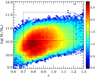
Figure 2.— Distribution of the ELGs as a function of redshift and stellar mass. The dotted lines show the redshift and stellar mass cuts of the sample used in this paper. We are selecting galaxies in the redshift range of $0.7<z<1.2$ and stellar mass range of $10<\log(M_{*}/M_{\sun})<11.6$. The color scales represent the logarithmic number counts at the redshift and stellar mass intervals.

The galaxy stellar mass is estimated for each object by performing the spectral energy distribution (SED) fitting to the photometry of $grz$ bands in DECaLs and the $W1W2$ bands in Wide-field Infrared Survey Explorer (WISE; Wright et al., 2010) with the FAST algorithm (Kriek et al., 2009), assuming the Chabrier (2003) IMF, the Bruzual & Charlot (2003) SPS model, and the dust attenuation law of Kriek & Conroy (2013) (full details are provided in Section 6.3 of Raichoor et al. 2017). In order to match the stellar mass estimates of G18 with the same IMF and SPS model assumptions but with the dust attenuation law of Charlot & Fall (2000), we increase the stellar mass in the ELG pipeline by 0.15 dex to take into account the difference in the dust attenuation laws, as found by Pérez-González et al. (2008) (see also Rodríguez-Puebla et al., 2017).

The star formation rates (SFRs) of the ELGs are also available from the SED fittings of the FAST code. We check the reliability of the output SFR values by comparing them to the SFR estimates from those galaxies with high S/N H$\alpha$ and H$\beta$ line fluxes. After applying the extinction correction using the Balmer decrement following the dust attenuation law of Charlot & Fall (2000) and also the aperture correction of the finite fiber diameter, we can estimate the SFR for these galaxies using the H$\alpha$ luminosity following Kennicutt (1998). We find that the SFR estimates from the FAST output and those from the H$\alpha$ luminosity are in good agreement with each other, with the average value of $\log(\rm{SFR}/M_{\sun}\,{\rm yr}^{-1})$ at $1<z<1.2$ being $1.63\pm 0.43$. As shown in Figure 1 of Lapi et al. (2017), the previous UV observations of the star-forming galaxies would considerably underestimate the SFR function for galaxies with SFRs larger than $30\,\rm{M_{\sun}}\,{\rm yr}^{-1}$ as a result of the strong dust extinction. Therefore, the eBOSS ELG observation provides a valuable sample of dusty star-forming galaxies with moderate SFRs at $z\sim 1$.

The stellar mass distribution of ELGs at different redshifts is displayed in Figure 2. As for any other ELG sample for measuring the baryon acoustic oscillations, the eBOSS ELG target selection aims to select a homogeneous sample of strong [O II] emitters with a given sky density within a given redshift range. As a consequence, the eBOSS ELG sample is not mass-complete. More massive ELGs are observed at higher redshifts by the g-band flux limits. In this paper, we focus on the redshift range of $0.7<z<1.2$ and only use the ELGs with $10<\log(M_{*}/M_{\sun})<11.6$. The redshift and stellar mass selection cuts are shown as the dotted lines in Figure 2.

In order to study the evolution of the SMF for the ELGs, we divide the sample into four redshift bins from $z=0.7$ to 1.2, with a bin size of $\Delta z=0.1$ for $z<1$ and a larger bin size of $1<z<1.2$ to achieve enough signal-to-noise (S/N) for the clustering measurements. We display the number of ELGs in each subsample, $N_{\rm tot}$, and the corresponding number densities, $\bar{n}_{\rm g}$, in Table 1.

Table 1Samples of Different Redshift Bins

Redshift Range	$N_{\rm tot}$	$\bar{n}_{\rm g}/(h^{3}\,\rm{Mpc}^{-3})$
$0.7<z<0.8$	61197	$3.61\times 10^{-4}$
$0.8<z<0.9$	71172	$3.66\times 10^{-4}$
$0.9<z<1.0$	37025	$1.71\times 10^{-4}$
$1.0<z<1.2$	24232	$0.49\times 10^{-4}$

Note. — The total number of galaxies and the average galaxy number densities of the eBOSS ELG samples at different redshifts are displayed.

2.2. Dark Matter Simulation

To apply the ICSMF model, we directly use the dark matter halo catalogs from the Multidark Planck simulation (MDPL; Klypin et al., 2016), with the cosmological parameters of $\Omega_{\rm m}=0.307$, $\Omega_{\rm b}=0.048$, $h=0.678$, $n_{\rm s}=0.96$ and $\sigma_{8}=0.823$. The simulation has a box size of $1\,h^{-1}{\rm{Gpc}}$ and a mass resolution of $1.5\times 10^{9}h^{-1}M_{\odot}$. The simulation resolution is high enough to resolve the host halos for the ELGs, which is around $10^{12}M_{\sun}$ (Favole et al., 2016). The dark matter halos and subhalos in the simulation are identified with the ROCKSTAR phase-space halo finder (Behroozi et al., 2013b). We use four different redshift outputs of $z=0.740$, 0.859, 0.944 and 1.077 from MDPL, roughly corresponding to the median redshifts of the four ELG subsamples.

3. Method

In this section, we briefly introduce the main ingredients of the ICSMF model of G18, which is based on the traditional conditional stellar mass function (CSMF) framework (see e.g., Yang et al., 2012; van den Bosch et al., 2013). By incorporating the stellar mass completeness, the ICSMF model is able to use the observed (incomplete) galaxy SMF and the two-point correlation function (2PCF) to simultaneously constrain the sample completeness and the galaxy SHMR. We refer the readers to G18 for more details.

3.1. ICSMF Model Ingredients

The three key ingredients of the ICSMF model are the CSMF, the SHMR and the stellar mass incompleteness. As in Yang et al. (2012) and G18, we assume a log-normal distribution for the central galaxy CSMF, i.e., the average number of central galaxies with stellar mass $M_{*}$ in host halos of given mass $M$,

$$\Phi_{\rm c}^{\rm sf}(M_{*}|M)=\frac{1}{\sqrt{2\pi}\sigma_{\rm*}}\exp\left[-\frac{(\log M_{*}-\log\langle M_{*}|M\rangle)^{2}}{2\sigma_{\rm*}^{2}}\right]$$ (7)

where $\sigma_{\rm*}$ characterizes the scatter of galaxy stellar mass at a given halo mass and the function $\langle M_{*}|M\rangle$ is the average central galaxy stellar mass in halos of mass $M$, i.e. the SHMR. Following Yang et al. (2012), we assume a constant scatter $\sigma_{\rm*}$ of $\max(0.173,0.2z)$ at a given redshift $z$ and the functional form for $\langle M_{*}|M\rangle$ is assumed to be a broken power law, (Yang et al., 2009; Wang & Jing, 2010)

$$\langle M_{*}|M\rangle=M_{*,0}\frac{(M/M_{1})^{\alpha+\beta}}{(1+M/M_{1})^{\beta}}$$ (8)

where $M_{*,0}$, $M_{1}$, $\alpha$, and $\beta$ are the four model parameters. The values of $\alpha+\beta$ and $\alpha$ represent the slopes of the low- and high-mass ends of the SHMR, respectively.

In G18, the stellar mass completeness is decomposed into the contributions from the central and satellite galaxies. After trying the model as in G18, we find that for the eBOSS ELG samples, the separate contributions of the central and satellite completeness functions are not well constrained, and they have similar completeness functions. Therefore, in this paper, we only assume an overall stellar mass completeness function, $c(M_{*})$, for all galaxies, as follows (Leauthaud et al., 2016),

$$c(M_{*})=\frac{f_{\rm c}}{2}\left[1+{\rm erf}\left(\frac{\log M_{*}-\log M_{\rm*,c}}{\sigma_{\rm c}}\right)\right]$$ (9)

where $\rm{erf}$ is the error function and the three free parameters are $f_{\rm c}$, $M_{\rm*,c}$, and $\sigma_{\rm c}$.

In G18, the ICSMF model was applied to the galaxies in the SDSS-III Baryon Oscillation Spectroscopic Survey (BOSS; Dawson et al., 2013) at $0.1<z<0.8$ for $10^{11}M_{\sun}<M_{\ast}<10^{12}M_{\sun}$, where the red/quiescent galaxies dominate the galaxy SMF. However, for the eBOSS ELG sample, the galaxy stellar mass spans two orders of magnitudes from $10^{10}M_{\sun}$ to $10^{12}M_{\sun}$, where the star-forming galaxies are not always dominating the entire galaxy population. In order to properly model the eBOSS ELGs that are mostly star-forming galaxies (Zhu et al., 2015; Comparat et al., 2016a), we need to quantify the number of star-forming galaxies in a given halo, which requires the measurements for the quiescent galaxies. Since the fraction of quiescent galaxies (i.e., quenched fraction) does not have a strong evolution in $0.7<z<1.2$ (see e.g., Moustakas et al., 2013; Muzzin et al., 2013; Tomczak et al., 2014), it is possible to constrain the quenched fraction using both the eBOSS ELGs and the BOSS LRGs in the overlap redshift range of $0.7<z<0.8$.

Here, we assume that the quenched fraction $f_{\rm q}$ is a function of the host halo mass (Tinker et al., 2013; Rodríguez-Puebla et al., 2015; Zu & Mandelbaum, 2016), which provides more flexiblity in the modeling as the star-forming and quenched galaxies could have different SHMRs. We adopt a similar functional form as in Peng et al. (2012) and Rodríguez-Puebla et al. (2015) for quenched ($f_{\rm q}$) and star-forming galaxies ($f_{\rm sf}$) as follows,

$$f_{\rm q}(M) = \frac{1}{1+M/M_{\rm q}},$$ (10)

$$f_{\rm sf}(M) = 1-f_{\rm q}(M)$$ (11)

The free parameter $M_{\rm q}$ characterizes the mass scale where half of the halos at a given mass $M$ contain quenched central galaxies. We note that with the incorporation of the quenched fraction, $c(M_{*})$ is just the completeness function relative to the star-forming galaxy population, but not to the whole population. We will adopt the same value of $M_{\rm q}$ constrained by the joint modeling of the eBOSS ELGs and BOSS LRGs in $0.7<z<0.8$ for all higher redshift samples, as will be detailed in §4.1.

3.2. Modeling the 2PCF Measurements

With the above four ingredients, we are able to predict the incomplete halo (subhalo) occupation functions for the central (satellite) ELGs in the stellar mass range of $M_{*,1}<M_{*}<M_{*,2}$, as

$$\langle N_{\rm c}(M)\rangle = \int_{M_{*,1}}^{M_{*,2}}\Phi_{\rm c}^{\rm sf}(M_{*}|M)c(M_{*})f_{\rm sf}(M)dM_{*}$$ (12)

$$\langle N_{\rm s}(M_{\rm acc})\rangle = \int_{M_{*,1}}^{M_{*,2}}\Phi_{\rm c}^{\rm sf}(M_{*}|M_{\rm acc})c(M_{*})f_{\rm sf}(M_{\rm acc})dM_{*}$$

where the subscripts ‘c’ and ‘s’ are for the central and satellite galaxies, respectively, and $M_{\rm acc}$ is the subhalo mass at the last accretion epoch. We have assumed that the satellite galaxies have the same CSMF as the centrals when they are distinct halos at the last accretion epoch. The possible evolution of $\Phi_{\rm c}^{\rm sf}(M_{*}|M)$ and the satellite galaxy stellar mass after accretion has been ignored (see Yang et al., 2012, for a more sophisticated model).

To compare with the traditional halo occupation distribution (HOD) (see e.g., Zheng et al., 2005, 2007; Zehavi et al., 2011), we can estimate the occupation function of the satellite galaxies in the host halo, $\langle N_{\rm s}(M)\rangle$, as follows:

$$\langle N_{\rm s}(M)\rangle = \int_{M_{*,1}}^{M_{*,2}}\Phi_{\rm s}^{\rm sf}(M_{*}|M)c(M_{*})f_{\rm sf}(M)dM_{*}$$ (14)

$$\Phi_{\rm s}^{\rm sf}(M_{*}|M) = \int dM_{\rm acc}\Phi_{\rm c}^{\rm sf}(M_{*}|M_{\rm acc})n_{\rm s}(M_{\rm acc}|M)\,,$$ (15)

where $\Phi_{\rm s}^{\rm sf}(M_{*}|M)$ is the CSMF for the satellite galaxies and $n_{\rm s}(M_{\rm acc}|M)$ is the subhalo mass function in host halos of mass $M$.

With the central and satellite HODs, the galaxy 2PCFs and the observed ELG SMFs can be predicted with the MDPL halo and subhalo catalogs in order to constrain the model parameters. We apply the efficient simulation-based method of Zheng & Guo (2016) to compute the 3D galaxy 2PCF, $\xi(r_{\rm p},r_{\rm\pi})$, where $r_{\rm\pi}$ and $r_{\rm p}$ are the separations of galaxy pairs along and perpendicular to the line of sight (LOS).

In more detail, the 3D galaxy 2PCF $\xi({\mathbf{r}})$ is measured as

$$\xi({\mathbf{r}})=\sum_{i,j}\frac{n_{{\rm h},i}n_{{\rm h},j}}{\bar{n}_{\rm g}^{2}}\langle N_{\rm c}(M_{i})\rangle\langle N_{\rm c}(M_{j})\rangle\xi_{\rm hh}({\mathbf{r}};M_{i},M_{j})$$

$$+ \sum_{i,j}2\frac{n_{{\rm h},i}n_{{\rm s},j}}{\bar{n}_{\rm g}^{2}}\langle N_{\rm c}(M_{i})\rangle\langle N_{\rm s}(M_{{\rm acc},j})\rangle\xi_{\rm hs}({\mathbf{r}};M_{i},M_{{\rm acc},j})$$

$$+ \sum_{i,j}\frac{n_{{\rm s},i}n_{{\rm s},j}}{\bar{n}_{\rm g}^{2}}\langle N_{\rm s}(M_{{\rm acc},i})\rangle\langle N_{\rm s}(M_{{\rm acc},j})\rangle\xi_{\rm ss}({\mathbf{r}};M_{{\rm acc},i},M_{{\rm acc},j})$$

where $n_{\rm h}(M)$ and $n_{\rm s}(M_{\rm acc})$ are the halo and subhalo mass functions, respectively, with $i$ and $j$ for different halo mass bins. The galaxy number density $\bar{n}_{\rm g}$ is computed as

$$\bar{n}_{\rm g}=\sum_{i}\left[\langle N_{\rm c}(M_{i})\rangle n_{\rm h}(M_{i})+\langle N_{\rm s}(M_{{\rm acc},i})\rangle n_{\rm s}(M_{{\rm acc},i})\right].$$ (17)

The 3D 2PCFs $\xi_{\rm hh}({\mathbf{r}};M_{i},M_{j})$, $\xi_{\rm hs}({\mathbf{r}};M_{i},M_{{\rm acc},j})$, and $\xi_{\rm ss}({\mathbf{r}};M_{{\rm acc},i},M_{{\rm acc},j})$ are the tabulated 2PCFs of the halo–halo, halo–subhalo, and subhalo–subhalo pairs, measured directly in the simulation.

To reduce the effect of redshift-space distortion (RSD), we focus on the measurements of the projected 2PCF $w_{\rm p}(r_{\rm p})$ (Davis & Peebles, 1983), defined as

$$w_{\rm p}(r_{\rm p})=2\int_{0}^{r_{\rm\pi,max}}\xi(r_{\rm p},r_{\rm\pi})dr_{\rm\pi},$$ (18)

where $r_{\rm\pi,max}$ is the maximum LOS distance to achieve the best S/N.

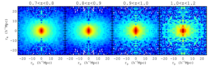
Figure 3.— Measurements of the 3D 2PCF $\xi(r_{\rm p},r_{\rm\pi})$ for the eBOSS ELGs at different redshifts. Despite the noisy signals on large scales, the small-scale Fingers-of-God and large-scale Kaiser squashing effects are clearly shown. Most of the clustering signals are contained in the LOS distance of $20\,h^{-1}{\rm{Mpc}}$, which is set as the maximum integration distance of the projected 2PCF measurements.

3.3. Modeling Observed Galaxy SMFs

By decomposing it into the central and satellite contributions, the observed (incomplete) galaxy SMF of the ELGs can be predicted to be

$$\Phi_{\rm sf}(M_{*}) = \Phi_{\rm sf,c}(M_{*})+\Phi_{\rm sf,s}(M_{*})$$ (19)

$$\Phi_{\rm sf,c}(M_{*}) = \int dM\Phi_{\rm c}^{\rm sf}(M_{*}|M)c(M_{*})f_{\rm sf}(M)n_{\rm h}(M)$$ (20)

$$\Phi_{\rm sf,s}(M_{*}) = \int dM_{\rm acc}\Phi_{\rm c}^{\rm sf}(M_{*}|M_{\rm acc})c(M_{*})\times$$ (21)

$$\quad\quad f_{\rm sf}(M_{\rm acc})n_{\rm s}(M_{\rm acc})$$

In summary, we have four free parameters ($M_{*,0}$, $M_{1}$, $\alpha$, and $\beta$) for the SHMR (Eq. 8), another three parameters ($f_{\rm c}$, $M_{\rm*,c}$, $\sigma_{\rm c}$) for the incompleteness component, and one parameter ($M_{\rm q}$) for the quenched fraction. The predictions of $w_{\rm p}(r_{\rm p})$ and $\Phi_{\rm sf}(M_{*})$ can be compared with those measured in the observed galaxy samples to obtain the best-fitting model parameters.

3.4. Observational Measurements

The 3D galaxy 2PCF $\xi(r_{\rm p},r_{\rm\pi})$ and the projected 2PCF $w_{\rm p}(r_{\rm p})$ for the ELGs are measured with the Landy–Szalay estimator (Landy & Szalay, 1993). We show in Figure 3 the measurements of $\xi(r_{\rm p},r_{\rm\pi})$ for samples at the different redshifts. Although the measurements of $\xi(r_{\rm p},r_{\rm\pi})$ are noisy on most scales, there are apparent Fingers-of-God (Jackson, 1972) and Kaiser squashing effects (Kaiser, 1987) on small and large scales, respectively. Similar to the measurements of Guo et al. (2013) for BOSS galaxies at $z\sim 0.55$, most of the clustering signals for the ELGs are located within an LOS distance of $20\,h^{-1}{\rm{Mpc}}$. Therefore, in order to achieve the best S/N ratio especially for the high-redshift ELG samples, we only integrate $\xi(r_{\rm p},r_{\rm\pi})$ to $r_{\pi,{\rm max}}=20\,h^{-1}{\rm{Mpc}}$ for the measurements of $w_{\rm p}(r_{\rm p})$. The residual RSD effect is taken into account in the theoretical model predictions with the same LOS distance in Eq. 18.

We choose logarithmic $r_{\rm p}$ bins with a width $\Delta\log r_{\rm p}=0.2$ from $1$ to $63.1\,h^{-1}{\rm{Mpc}}$, and linear $r_{\rm\pi}$ bins of width $\Delta r_{\rm\pi}=2\,h^{-1}{\rm{Mpc}}$ from 0 to 20$\,h^{-1}{\rm{Mpc}}$. We measure the projected 2PCFs for the three stellar mass bins from $M_{*}=10^{10}M_{\sun}$ to $10^{11.5}M_{\sun}$ with a bin size of $\Delta\log M_{*}=0.5$ at different redshifts. The observed SMF $\Phi_{\rm sf}(M_{*})$ is measured in the stellar mass range of $10^{10}M_{\sun}<M_{*}<10^{11.6}M_{\sun}$ with a logarithmic width of $\Delta\log M_{*}=0.2$.

3.5. ICSMF Model Constraints

We estimate the error covariance matrices for $w_{\rm p}(r_{\rm p})$ and $\Phi_{\rm sf}(M_{*})$ using the jackknife resampling technique with 100 subsamples as in G18. The cross-covariance between the $w_{\rm p}(r_{\rm p})$ measurements for the different stellar mass bins are also taken into account in the full covariance matrix. We only use the diagonal elements of the covariance matrix of $\Phi_{\rm sf}$, as the uncertainties from the systematic effects of the stellar mass measurements are hard to estimate (Mitchell et al., 2013). The contribution of Poisson noise to the observed ELG SMF is added in quadrature to $\sigma_{\Phi_{\rm sf}}$.

We apply a Markov Chain Monte Carlo (MCMC) method to fully explore the model parameter space. The probability likelihood surface is determined by $\chi^{2}$ as follows:

$$\chi^{2} = \chi^{2}_{w_{\rm p}}+\frac{(\Phi_{\rm sf}-\Phi_{\rm sf}^{*})^{2}}{\sigma_{\Phi_{\rm sf}}^{2}}$$ (22)

$$\chi^{2}_{w_{\rm p}} = (\mathbf{w_{\rm p}}-\mathbf{w_{\rm p}^{*}})^{T}\mathbf{C}_{w_{\rm p}}^{-1}(\mathbf{w_{\rm p}}-\mathbf{w_{\rm p}^{*}}),$$ (23)

where $\mathbf{C}_{w_{\rm p}}$ is the full error covariance matrix of $w_{\rm p}(r_{\rm p})$. The quantity with (without) a superscript ‘$*$’ is the one from the data (model).

3.6. ICSMF Model Predictions

With the best-fitting model constraints, we can also infer other properties of the ELG samples, e.g., the galaxy bias, the satellite fraction and the intrinsic galaxy SMFs. The galaxy bias for the stellar mass range of $M_{*,1}<M_{*}<M_{*,2}$ can be directly estimated as (van den Bosch et al., 2013),

$$b_{\rm g}(M_{*}) = \frac{1}{\bar{n}_{\rm g}}\int dM\langle N(M)\rangle n_{\rm h}(M)b_{\rm h}(M)$$ (24)

$$\langle N(M)\rangle = \langle N_{\rm c}(M)\rangle+\langle N_{\rm s}(M)\rangle.$$ (25)

We adopt the halo bias fitting function of Tinker et al. (2010) for $b_{\rm h}(M)$ (see also Comparat et al., 2017a) and $\langle N(M)\rangle$ is the average halo occupation number for galaxies in this stellar mass bin. The average galaxy bias $\langle b_{\rm g}\rangle$ of each galaxy sample can be obtained by using the halo occupation numbers for the whole stellar mass range in Equations. 12 and  LABEL:eq:nsat_int.

The satellite galaxy fraction, $f_{\rm sat}(M_{*})$, in the observed ELG sample can be estimated as,

$$f_{\rm sat}(M_{*})=\Phi_{\rm sf,s}(M_{*})/\Phi_{\rm sf}(M_{*}),$$ (26)

The average satellite fraction of the whole galaxy sample at a given redshift interval is

$$\langle f_{\rm sat}\rangle=\frac{\int dM_{*}\Phi_{\rm sf,s}(M_{*})}{\int dM_{*}\Phi_{\rm sf}(M_{*})}\,.$$ (27)

Most importantly, we can infer the intrinsic galaxy SMF for the star-forming population, $\tilde{\Phi}_{\rm sf}(M_{*})$, to be

$$\tilde{\Phi}_{\rm sf}(M_{*})=\int dM\Phi_{\rm c}^{\rm sf}(M_{*}|M)f_{\rm sf}(M)n_{\rm h}(M)$$

$$+\int dM_{\rm acc}\Phi_{\rm c}^{\rm sf}(M_{*}|M_{\rm acc})f_{\rm sf}(M_{\rm acc})n_{\rm s}(M_{\rm acc})\,.$$ (28)

We can further predict the intrinsic galaxy SMF for the quenched galaxies, $\tilde{\Phi}_{\rm q}(M_{*})$, and that of the total population, $\tilde{\Phi}(M_{*})$, as,

$$\tilde{\Phi}_{\rm q}(M_{*})=\int dM\Phi_{\rm c}^{\rm q}(M_{*}|M)f_{\rm q}(M)n_{\rm h}(M)$$

$$\quad+\int dM_{\rm acc}\Phi_{\rm c}^{\rm q}(M_{*}|M_{\rm acc})f_{\rm q}(M_{\rm acc})n_{\rm s}(M_{\rm acc})$$ (29)

$$\tilde{\Phi}(M_{*})=\tilde{\Phi}_{\rm sf}(M_{*})+\tilde{\Phi}_{\rm q}(M_{*}),$$ (30)

where we have assumed different conditional stellar mass functions, $\Phi_{\rm c}^{\rm sf}(M_{*}|M)$ and $\Phi_{\rm c}^{\rm q}(M_{*}|M)$, for tje star-forming and quenched galaxies, respectively.

In principle, the quenched and star-forming galaxies can have different SHMRs. However, the level of differences is still under debate in the literature, even for the well-measured galaxy populations from the SDSS main galaxy sample at $z\sim 0$ (see Wechsler & Tinker, 2018, for a review and references therein, especially their Figure 10). It is still not quite clear whether the SHMRs of the star-forming and quenched galaxies are significantly different from each other at high redshifts (see e.g., Tinker et al., 2013, for an analysis using samples with photometric redshifts). In this study, with both the eBOSS ELGs and BOSS LRGs at the same redshift range of $0.7<z<0.8$, we are able to discriminate the possible differences between the CSMFs of the two populations.

4. Results

4.1. Fitting the Observables via two steps

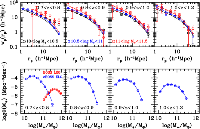
Figure 4.— Projected 2PCF measurements (upper panels) and the observed SMFs (lower panels) for the eBOSS ELGs at $0.7<z<1.2$. In the upper panels, the symbols with different colors represent the $w_{\rm p}(r_{\rm p})$ for the different stellar mass bins as labeled, and the corresponding solid lines are the best-fitting models. In the lower panels, the observed SMF measurements and the best-fitting models are shown as the symbols and lines, respectively. For the redshift bin of $0.9<z<1$, only nine data points are shown, as there are no observed ELGs in the largest stellar mass bin. Our best-fitting models are in very good agreement with the observed clustering and SMF measurements.

Figure 5.— Best-fitting quenched fraction as a function of halo mass $M$ (open circles with errors).

We show in Figure 4 the projected 2PCF measurements (upper panels) and the observed SMFs (lower panels) for the eBOSS ELGs at $0.7<z<1.2$. In the upper panels, the symbols of different colors are for the ELGs in the different stellar mass bins. The clustering amplitudes of $w_{\rm p}(r_{\rm p})$ for the two stellar bins of $\log(M_{*}/M_{\sun})<11$ almost overlap with each other, reflecting the flattening trend of the galaxy bias at the lower mass end, similar to the situation in the SDSS main galaxy sample (see e.g., Li et al., 2006; Zehavi et al., 2011). The observed ELG SMFs (blue circles) are shown in the lower panel of Figure 4.

Before we fit to the data in all redshift bins, as we pointed out in §3.1, the quenched fraction $f_{\rm q}(M)$ can be properly constrained by jointly modeling the eBOSS ELG and BOSS LRG samples. As these data are available only in the redshift interval of $0.7<z<0.8$, we first focus on this redshift bin to make our model constraints.

Table 2Best-fitting Model Parameters

Parameter	$0.7<z<0.8$	$0.8<z<0.9$	$0.9<z<1.0$	$1.0<z<1.2$
$\chi^{2}/{\rm dof}$	$118.22/48$	$25.52/28$	$48.43/28$	$46.16/28$
$\log(M_{*,0}/M_{\sun})$	$10.231^{+0.233}_{-0.087}$	$11.006^{+0.046}_{-0.310}$	$11.090^{+0.014}_{-0.122}$	$11.199^{+0.016}_{-0.113}$
$\log(M_{1}/M_{\sun})$	$10.893^{+0.127}_{-0.168}$	$11.342^{+0.008}_{-0.202}$	$11.408^{+0.046}_{-0.080}$	$11.454^{+0.015}_{-0.120}$
$\alpha$	$0.346^{+0.003}_{-0.120}$	$0.020^{+0.144}_{-0.020}$	$0.007^{+0.066}_{-0.007}$	$0.007^{+0.067}_{-0.007}$
$\beta$	$7.729^{+0.489}_{-0.024}$	$8.094^{+0.596}_{-0.726}$	$8.574^{+0.173}_{-1.089}$	$8.610^{+0.157}_{-1.038}$
$\log f_{\rm c}$	$-1.276^{+0.117}_{-0.205}$	$-1.188^{+0.142}_{-0.048}$	$-1.370^{+0.081}_{-0.067}$	$-1.888^{+0.025}_{-0.144}$
$\log(M_{\rm*,c}/M_{\sun})$	$10.216^{+0.108}_{-0.051}$	$10.151^{+0.260}_{-0.009}$	$10.295^{+0.062}_{-0.009}$	$10.315^{+0.026}_{-0.014}$
$\sigma_{\rm c}$	$0.235^{+0.308}_{-0.027}$	$0.323^{+0.329}_{-0.023}$	$0.287^{+0.064}_{-0.015}$	$0.232^{+0.029}_{-0.013}$
$\langle f_{\rm sat}\rangle$	$0.165^{+0.004}_{-0.004}$	$0.155^{+0.003}_{-0.002}$	$0.145^{+0.003}_{-0.003}$	$0.137^{+0.006}_{-0.001}$
$\langle b_{\rm g}\rangle$	$1.103^{+0.057}_{-0.027}$	$1.223^{+0.013}_{-0.026}$	$1.374^{+0.015}_{-0.062}$	$1.420^{+0.025}_{-0.036}$

Note. — The average satellite fraction $\langle f_{\rm sat}\rangle$ and average galaxy bias $\langle b_{\rm g}\rangle$ of the ELG samples at each redshift interval are also displayed.

Following G18, the BOSS LRG is selected from the Data Release 12 of the BOSS galaxy sample (Reid et al., 2016), by applying the additional color selection of $g-i>2.35$ to remove the blue/star-forming galaxies as proposed in Masters et al. (2011) (see also Maraston et al., 2013). The clustering measurements for BOSS LRGs are presented in two stellar mass bins of $11<\log(M_{*}/M_{\sun})<11.5$ and $11.5<\log(M_{*}/M_{\sun})<12$, while the SMF is measured in $11<\log(M_{*}/M_{\sun})<12$ with a bin size of $\Delta\log M_{*}=0.1$. We refer the readers to Section 2.1 of G18 for more details of the BOSS galaxy sample. As a reference, the SMF measurement of the BOSS LRGs at $0.7<z<0.8$ is also shown in the lower-left panel of Figure 4 as the red circles. Obviously, the high-mass end of the galaxy SMF is dominated by the quenched (red) galaxies.

As the BOSS LRGs were observed with completely different target selections from those of the eBOSS ELGs, and to see whether they have different $\Phi_{\rm c}^{\rm q}(M_{*}|M)$ from $\Phi_{\rm c}^{\rm sf}(M_{*}|M)$, we use another four parameters ($M_{*,0}^{\prime}$, $M_{1}^{\prime}$, $\alpha^{\prime}$, $\beta^{\prime}$) for the SHMR of the BOSS LRGs as in Equation (8) and three parameters ($f_{\rm c}^{\prime}$, $M_{\rm*,c}^{\prime}$, $\sigma_{\rm c}^{\prime}$) for the LRG stellar mass completeness function as in Equation (9). The observed galaxy clustering and SMF measurements of the BOSS LRGs can be modeled by replacing $f_{\rm sf}(M)$ with $f_{\rm q}(M)$ in Equations  (12)–(21).

With all of these data and models available for galaxies in the redshift interval of $0.7<z<0.8$, we proceed to make our model constraints using the MCMC method. The best-fitting quenched fraction $f_{\rm q}(M)$ is shown as the open circles in Figure 5, with the best-fitting value of $\log(M_{\rm q}/M_{\sun})=12.83\pm 0.24$, which is in good agreement with that obtained in Tinker et al. (2013) (their Figure 9).

Assuming that this quenched fraction $f_{\rm q}(M)$ with the best-fitting value of $\log(M_{\rm q}/M_{\sun})=12.83$ will not evolve significantly, which is also supported by the lack of evolution of $f_{\rm q}(M_{*})$ from the literature, in our second step, we proceed to make our model constraints for the eBOSS ELGs in the redshift range of $0.8<z<1.2$.

We show in Figure 4 the best-fitting models using the corresponding solid lines for $w_{\rm p}(r_{\rm p})$ (upper panels) and SMF (lower panels), respectively. Our best-fitting models show very good agreement with the measured $w_{\rm p}(r_{\rm p})$ at all redshifts and stellar mass bins. In addition, given the small errors of the SMF measurements, the good agreement between the two demonstrates that our functional form of the stellar mass completeness is reasonable.

Finally, the best-fitting model parameters are displayed in Table 2, where the average satellite fraction $\langle f_{\rm sat}\rangle$ and average galaxy bias $\langle b_{\rm g}\rangle$ at each redshift interval are also given. In addition to these fiducial modeling and fitting, we have also tested some alternatives to quenching and scatter modeling to check the robustness of our results, which are provided in the Appendix.

4.2. Model constraints

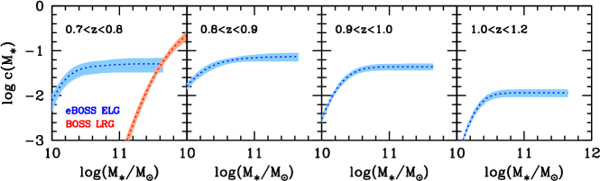
Figure 6.— Best-fitting stellar mass completeness functions, $c(M_{*})$, for the eBOSS ELGs from $z=0.7$ to $z=1.2$ (blue dotted line in each panel). The shaded regions are the corresponding error distributions. The constraints to the completeness function of the BOSS LRGs at $0.7<z<0.8$ is also shown as the red dotted line with the shaded area.

Table 3Completeness Functions $\log c(M_{*})$ for eBOSS ELGs

$\log(M_{*}/M_{\sun})$	$0.7<z<0.8$	$0.8<z<0.9$	$0.9<z<1.0$	$1.0<z<1.2$
10.0	$-1.977^{+0.129}_{-0.185}$	$-1.707^{+0.065}_{-0.077}$	$-2.331^{+0.064}_{-0.076}$	$-3.204^{+0.082}_{-0.101}$
10.2	$-1.563^{+0.114}_{-0.154}$	$-1.445^{+0.072}_{-0.087}$	$-1.789^{+0.059}_{-0.069}$	$-2.415^{+0.068}_{-0.080}$
10.4	$-1.399^{+0.114}_{-0.155}$	$-1.293^{+0.065}_{-0.077}$	$-1.506^{+0.060}_{-0.069}$	$-2.054^{+0.069}_{-0.083}$
10.6	$-1.349^{+0.118}_{-0.163}$	$-1.215^{+0.056}_{-0.064}$	$-1.396^{+0.059}_{-0.069}$	$-1.954^{+0.073}_{-0.088}$
10.8	$-1.323^{+0.121}_{-0.168}$	$-1.175^{+0.060}_{-0.070}$	$-1.364^{+0.065}_{-0.076}$	$-1.940^{+0.076}_{-0.092}$
11.0	$-1.303^{+0.126}_{-0.177}$	$-1.152^{+0.071}_{-0.085}$	$-1.358^{+0.067}_{-0.080}$	$-1.940^{+0.076}_{-0.092}$
11.2	$-1.294^{+0.130}_{-0.187}$	$-1.140^{+0.078}_{-0.096}$	$-1.357^{+0.068}_{-0.081}$	$-1.940^{+0.076}_{-0.092}$
11.4	$-1.294^{+0.130}_{-0.187}$	$-1.134^{+0.082}_{-0.101}$	$-1.357^{+0.068}_{-0.081}$	$-1.940^{+0.076}_{-0.092}$
11.6	$-1.291^{+0.131}_{-0.189}$	$-1.132^{+0.084}_{-0.104}$	$-1.357^{+0.068}_{-0.081}$	$-1.940^{+0.076}_{-0.092}$

Note. — The measurements are shown for the completeness function, $\log c(M_{*})$, of the whole ELG samples at different redshifts, as defined in Eq. (9).

After we constrain our models as outlined in Section 4.1, we provide the related model constraints in this subsection.

4.2.1 Stellar Mass Completeness

We show in Figure 6 the best-fitting stellar mass completeness functions at different redshifts as the blue dotted lines, with the shaded regions as the 1$\sigma$ error distributions. As seen from the figure, as a result of the complicated target selections, the eBOSS ELG sample is very incomplete, with the average high-mass end completeness varying from about 1% to 10% depending on the redshift. The BOSS LRG sample completeness at $0.7<z<0.8$ is shown as the red dotted line with the shaded area in the leftmost panel. The BOSS LRG sample is more complete at the massive end where they dominate the galaxy SMF.

The ELG samples at lower redshifts are relatively more complete than the higher redshift ones, as the target selection cuts are designed to choose galaxies in the redshift range of $0.7<z<1.1$ (see Figure 4 of Raichoor et al., 2017). The completeness of the ELG samples decreases significantly toward the low-mass end. For galaxies with stellar mass around $10^{10}M_{\sun}$, the eBOSS ELG sample only consists of less than 1% of the star-forming galaxy population. The values of the stellar mass completeness for eBOSS ELGs are listed in Table 3. We caution that the low completeness of the eBOSS ELGs makes them less representative of the entire star-forming galaxy population, which can be improved with the next-generation ELG surveys with higher completenesses as in DESI (see e.g., Gonzalez-Perez et al., 2018).

Thanks to the large sky coverage of the eBOSS ELG program, as shown in Table 1, we have a reasonable number of galaxies at $z\sim 1$ to achieve accurate clustering measurements, despite of the low sampling rates. While the clustering measurements only weakly depend on the sample completeness as shown in Equations (LABEL:eq:xicc_sim) and (17), the remaining question is whether the observed [O II] emitters are a representative subsample of the overall star-forming galaxy population. By comparing to the SFR vs. stellar mass relation in Figure 1 of Moustakas et al. (2013) at similar redshifts, we find that the eBOSS ELG sample is selecting typical star-forming galaxies that lie within the star-formation sequence, with the mean $\log(\rm{SFR}/M_{\sun}\,{\rm yr}^{-1})$ at $0.65<z<0.8$ and $0.8<z<1.0$ being $0.89\pm 0.42$ and $1.22\pm 0.45$, respectively. As will be shown in §4.3.1, it is also encouraging that the recovered intrinsic galaxy SMFs are in good agreement with the literature, further confirming that the eBOSS ELGs are in general representative of the star-forming populations at the corresponding redshifts.

4.2.2 Stellar-Halo Mass Relation

We show in the top panels of Figure 7 the predicted SHMRs of ELGs as the blue circles with errors. The SHMR of the BOSS LRG in $0.7<z<0.8$ is shown as the red circles in the left most panel. There is only weak evolution in the shape of the ELG SHMR from $z=1.2$ to $z=0.7$ for halos of $\log(M/M_{\sun})<13$. The high-mass end slope $\alpha$ of the SHMR is around 0.35 at $0.7<z<0.8$, while it becomes very flat ($\alpha\sim 0$) for higher redshift samples. It implies that there are only very few star-forming galaxies of $M_{*}>10^{11.2}M_{\sun}$ at these redshifts. But the SMFs of the star-forming galaxies at the massive end are still not vanishing due to the large scatter $\sigma_{*}$ for the high redshift samples. However, we caution that the error on the best-fitting slope $\alpha$ may be underestimated in our model, as it is mainly constrained by the observed SMFs. The constraining power of the clustering measurements is weakened by the low S/N.

By comparing the SHMRs between the eBOSS ELG and BOSS LRG samples at $0.7<z<0.8$, we find that the ELGs and LRGs have very similar SHMRs for halos of $\log(M/M_{\sun})<12$. For more massive halos, there are significant differences between the two SHMRs, with the quiescent galaxies having a much steeper slope at the massive end as also shown in Figure 9 of G18. Tinker et al. (2013) have constrained the SHMRs for the quiescent and star-forming galaxies over the redshift range of $0.2<z<1$ by using measurements of the galaxy angular clustering and galaxy–galaxy lensing in the COSMOS field. For fair comparisons, we also show the results of Tinker et al. (2013) at $0.74<z<1$ as the red and blue solid lines for the quiescent and star-forming populations, respectively. The trend in the discrepancy between the two SHMRs is in good agreement with those of Tinker et al. (2013). They attributed the differences to the much larger scatter $\sigma_{*}$ of the star-forming galaxies in their models. However, in our model, we assume the same scatter $\sigma_{*}$ for both the star-forming and quiescent galaxies. Therefore, the differences in the SHMRs may reflect the intrinsic variation in the average galaxy stellar mass at a given halo mass for the two populations.

We note that the high mass end of the galaxy SMF is dominated by the quiescent galaxies. Since most previous results of the galaxy SHMR constraints come from fitting the overall galaxy SMFs (see e.g., Yang et al., 2012; Behroozi et al., 2013a; Moster et al., 2013; Rodríguez-Puebla et al., 2017), they are not directly comparable to our model predictions of the ELG SHMR at these redshifts.

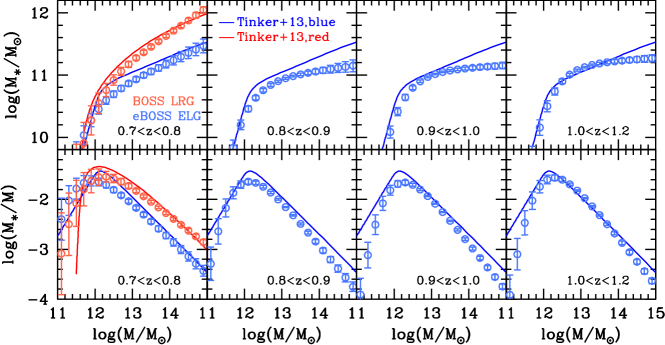
Figure 7.— Best-fitting stellar-halo mass relations (top panels) and the stellar-to-halo mass ratios (bottom panels). The blue open circles are for the eBOSS ELGs, with the red open circles for the BOSS LRG at $0.7<z<0.8$. The model results of Tinker et al. (2013) for red and blue galaxies (see text) are also shown for comparison as the red and blue solid lines.

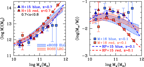
Figure 8.— Left: the model constraints to the average halo mass at a given stellar mass. The 1$\sigma$ ranges of our best-fitting models for the BOSS LRGs and eBOSS ELGs at $0.7<z<0.8$ are shown as the red and blue shaded regions, respectively. The weak lensing measurements from Hudson et al. (2015) (denoted as “H+15”) at $z\sim 0.7$ and Mandelbaum et al. (2016) (denoted as “M+16”) at $z\sim 0$ are shown as the filled triangles and squares, respectively. We also display the halo model predictions from Rodríguez-Puebla et al. (2015) (denoted as “RP+15”) at $z\sim 0$ for comparison. Right: the corresponding stellar-to-halo mass ratios of different measurements in the left panel.

We show in the bottom panels of Figure 7 the stellar-to-halo mass ratios as a function of the halo mass at different redshifts. The peaks of the stellar-to-halo mass ratio happen at around $M\sim 10^{12}M_{\sun}$, consistent with the findings in the literature (see e.g., Yang et al., 2012; Behroozi et al., 2013a). It is interesting that the peak locations of the stellar-to-halo mass ratios for the quiescent and star-forming galaxies are roughly coincident with each other. It implies that the transition from the star-forming to quiescent galaxies might be most efficient in halos of $M\sim 10^{12}M_{\sun}$.

To appropriately compare with the observational constraints from the weak lensing measurements, we also calculate the average halo masses at given stellar masses for star-forming and quiescent central galaxies as (Hudson et al., 2015; Rodríguez-Puebla et al., 2015),

$$\langle M|M_{*}\rangle_{\rm sf} = \frac{\int\Phi_{\rm c}^{\rm sf}(M_{*}|M)f_{\rm sf}(M)n_{\rm h}(M)MdM}{\int\Phi_{\rm c}^{\rm sf}(M_{*}|M)f_{\rm sf}(M)n_{\rm h}(M)dM}$$ (31)

$$\langle M|M_{*}\rangle_{\rm q} = \frac{\int\Phi_{\rm c}^{\rm q}(M_{*}|M)f_{\rm q}(M)n_{\rm h}(M)MdM}{\int\Phi_{\rm c}^{\rm q}(M_{*}|M)f_{\rm q}(M)n_{\rm h}(M)dM},$$ (32)

which are significantly different from the SHMR of $\langle M_{*}|M\rangle$ due to the existence of scatter $\sigma_{*}$, especially at the massive end (Behroozi et al., 2010; Tinker et al., 2013). As we only have the measurements of both LRGs and ELGs at $0.7<z<0.8$, we show our best-fitting model constraints to $\langle M|M_{*}\rangle_{\rm sf}$ and $\langle M|M_{*}\rangle_{\rm q}$ in the left panel of in Figure 8, while the stellar-to-halo mass ratios for the two samples as a function of the stellar mass are shown in the right panel. For comparison, we also display the galaxy-galaxy weak lensing measurements for red and blue galaxies from Hudson et al. (2015) at $z\sim 0.7$ and from Mandelbaum et al. (2016) at $z\sim 0$. The halo model constraints from Rodríguez-Puebla et al. (2015) at $z\sim 0$ are also shown as the dotted lines.

Our model predictions of the $\langle M|M_{*}\rangle$ for star-forming and quiescent galaxies almost overlap with each other over the stellar mass range of $10<\log(M_{*}/M_{\sun})<12$ at $0.7<z<0.8$, consistent with the results of Tinker et al. (2013) (their Figure 7). Compared to the weak lensing measurements from Hudson et al. (2015), our model predictions tend to be slightly higher. However, as noted by Coupon et al. (2015) (their Figure 11), the stellar mass measurements of Hudson et al. (2015) are likely biased high due to the lack of NIR data and the estimated halo mass is dependent on the details of modeling the contributions of subhalos in the lensing signals. The low redshift measurements of Mandelbaum et al. (2016) and Rodríguez-Puebla et al. (2015) agree well with each other. They found apparent differences in the halo masses for red and blue galaxies with the same stellar masses, considering the small errors in the red galaxy measurements. Although such a trend is not shown in our best-fitting model constraints at $z\sim 0.7$, the overall evolution of $\langle M|M_{*}\rangle$ is generally weak, especially for galaxies with $\log(M_{*}/M_{\sun})<11$. As pointed out by Lapi et al. (2018a), the weak evolution of the mass ratio $\langle M_{*}/M\rangle$ for low mass galaxies indicates the joint effects of the star formation and dark matter accretion along the cosmic time, which would have important constraints on the galaxy formation and evolution models, while the evolution of more massive galaxies may be quite different (Shankar et al., 2014; Bernardi et al., 2016; Lapi et al., 2018b).

4.3. Model predictions

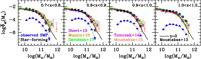
Figure 9.— Intrinsic stellar mass functions for the star-forming galaxies. The black circles are our best-fitting models, while crosses of different colors represent the previous measurements of Ilbert et al. (2013), Muzzin et al. (2013), Moustakas et al. (2013), Tomczak et al. (2014) and Davidzon et al. (2017). We note that the measurements of previous literature are in much larger redshift bins compared to our results. They are repeated in some neighboring bins for simple comparisons. The measurements at the low redshifts of $z\sim 0$ from Moustakas et al. (2013) are also shown as the black solid line in each panel for comparisons. The dotted line in each panel shows the observed eBOSS ELG SMF.

With the above model constraints, as we outlined in Section 3.6, it is quite straightforward to make some model predictions, such as the intrinsic galaxy SMFs, the HOD, the galaxy bias and the satellite fraction.

4.3.1 Intrinsic Galaxy SMFs

We show in Figure 9 the predicted intrinsic galaxy SMFs as black open circles for the star-forming galaxies from our best-fitting models. The measurements of the intrinsic SMFs for the star-forming galaxies are also displayed in Table 4. We show for comparison the previous measurements in the literature at the corresponding redshifts, including Ilbert et al. (2013), Moustakas et al. (2013), Muzzin et al. (2013), Tomczak et al. (2014) and Davidzon et al. (2017) as crosses of different colors. The local-universe measurements of Moustakas et al. (2013) at $z\sim 0$ are shown as the solid line in each panel to see the evolution effect. We have corrected the different assumptions of the IMF, SPS models and dust attenuation laws in the literature following Rodríguez-Puebla et al. (2017), to be consistent with our model assumptions. The blue open triangles are the observed galaxy SMFs as in Figure 4, with the dotted lines showing the best-fitting models.

Our best-fitting models for the intrinsic galaxy SMFs of the star-forming galaxies are generally in good agreement with the literature. While at the low-mass end ($M_{*}<10^{10}M_{\sun}$) the SMFs from the previous literature are roughly consistent with each other, there are larger discrepancies for more massive galaxies. As those previous measurements are made with photometric redshifts covering small but deep survey area, the variations could be caused by the sample variance effect due to the limited volumes and also other systematic effects, such as the different methods to estimate the galaxy stellar mass and to discriminate between the star-forming (blue) and quiescent (red) galaxies.

Table 4Intrinsic SMF $\log\tilde{\Phi}_{\rm sf}(M_{*})$ For Star-Forming Galaxies

$\log(M_{*}/M_{\sun})$	$0.7<z<0.8$	$0.8<z<0.9$	$0.9<z<1.0$	$1.0<z<1.2$
10.1	$-2.330^{+0.108}_{-0.145}$	$-2.462^{+0.065}_{-0.077}$	$-2.598^{+0.054}_{-0.062}$	$-2.610^{+0.066}_{-0.077}$
10.3	$-2.404^{+0.108}_{-0.144}$	$-2.503^{+0.063}_{-0.074}$	$-2.635^{+0.055}_{-0.063}$	$-2.646^{+0.066}_{-0.078}$
10.5	$-2.527^{+0.110}_{-0.149}$	$-2.568^{+0.059}_{-0.069}$	$-2.689^{+0.056}_{-0.065}$	$-2.694^{+0.068}_{-0.081}$
10.7	$-2.749^{+0.114}_{-0.156}$	$-2.698^{+0.055}_{-0.063}$	$-2.785^{+0.058}_{-0.067}$	$-2.768^{+0.071}_{-0.085}$
10.9	$-3.124^{+0.117}_{-0.161}$	$-2.975^{+0.060}_{-0.069}$	$-2.980^{+0.063}_{-0.074}$	$-2.903^{+0.075}_{-0.091}$
11.1	$-3.705^{+0.123}_{-0.171}$	$-3.503^{+0.073}_{-0.088}$	$-3.362^{+0.067}_{-0.080}$	$-3.156^{+0.077}_{-0.094}$
11.3	$-4.529^{+0.136}_{-0.199}$	$-4.374^{+0.084}_{-0.104}$	$-4.017^{+0.072}_{-0.086}$	$-3.593^{+0.078}_{-0.096}$
11.5	$-5.619^{+0.183}_{-0.321}$	$-5.650^{+0.092}_{-0.116}$	$-5.010^{+0.076}_{-0.093}$	$-4.267^{+0.078}_{-0.095}$

Note. — The stellar mass function measurements are in units of $\rm{Mpc}^{-3}\rm{dex}^{-1}$.

Table 5Best-fit Schechter Function Parameters for the ELGs

redshift range	$\log(\Phi^{\ast}/\rm{Mpc}^{-3}\rm{dex}^{-1})$	$\log(M^{\ast}_{\rm c}/M_{\sun})$	$\alpha^{\ast}$
$0.7<z<0.8$	$-2.658\pm 0.162$	$10.637\pm 0.077$	$-1.253\pm 0.328$
$0.8<z<0.9$	$-2.559\pm 0.039$	$10.585\pm 0.020$	$-0.791\pm 0.123$
$0.9<z<1.0$	$-2.793\pm 0.043$	$10.735\pm 0.018$	$-0.936\pm 0.095$
$1.0<z<1.2$	$-2.939\pm 0.059$	$10.938\pm 0.024$	$-1.071\pm 0.096$

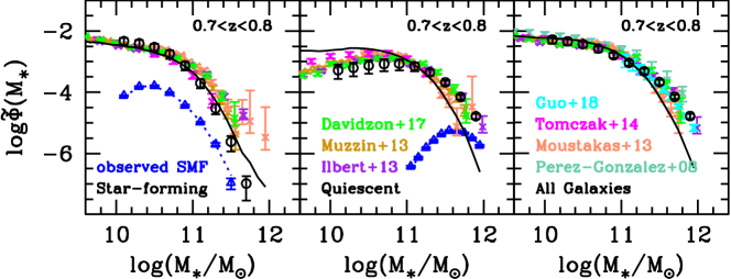
Figure 10.— Intrinsic stellar mass functions for the star-forming galaxies (left panel), quiescent galaxies (middle panel) and all galaxies (right panel) at $0.7<z<0.8$. The black circles are our best-fitting models, while crosses of different colors represent the measurements of Pérez-González et al. (2008), Ilbert et al. (2013), Muzzin et al. (2013), Moustakas et al. (2013), Tomczak et al. (2014), Davidzon et al. (2017) and G18. The black solid lines are the measurements at $z\sim 0$ from Moustakas et al. (2013). The open triangles with the dotted lines are the observed eBOSS ELG SMF and the corresponding best-fitting models. For comparison purposes, we have extended our predicted galaxy SMFs over the whole stellar mass range of $10^{10}M_{\sun}<M_{*}<10^{12}M_{\sun}$.

As the eBOSS ELG sample covers a significantly larger volume than the previous surveys, it suffers less from the sample variance effect. In addition, the star-forming galaxies are identified with the [O II] emission line, which is more reliable than the discrimination method with the color-magnitude diagram used in previous surveys. However, we note that the stellar masses of the eBOSS ELGs are obtained with a small number of available bands in DECaLs and WISE. The stellar mass estimates from the SED fittings are therefore less accurate compared to the previous deep surveys with broadband photometry.

For the star-forming galaxy population, there is only weak evolution of the SMF at $M_{*}<10^{11}M_{\sun}$ from $z=1.2$ to $0.7$. Our best-fitting models predict that the number density of ELGs with $M_{*}>10^{11}M_{\sun}$ decreases significantly around $z\sim 1$. However, we caution that our model predictions at $z>1$ might be affected by the low sample selection rates ($\sim 1\%$) which make the observed ELGs less representative of the overall star-forming galaxy population. Compared to the SMF measurements of the star-forming galaxies at $z\sim 0$, it seems that there is almost no evolution from $z\sim 0$ to $z=0.9$, which is consistent with the conclusions of previous measurements as in Ilbert et al. (2013), Muzzin et al. (2013) and Lapi et al. (2017).

To quantitatively compare with the corresponding measurements in the literature, we also fit the intrinsic SMFs for the star-forming galaxies with the standard single Schechter function (Schechter, 1976),

$$\Phi(M_{*})=(\ln 10)\Phi^{\ast}\exp\left(-\frac{M_{*}}{M^{\ast}_{\rm c}}\right)\left(\frac{M_{*}}{M^{\ast}_{\rm c}}\right)^{1+\alpha^{\ast}}$$ (33)

The best-fit parameters $\Phi^{\ast}$, $M^{\ast}_{\rm c}$ and $\alpha^{\ast}$ are shown in Table 5.

As we have the measurements for both the quiescent and star-forming galaxies at $0.7<z<0.8$, we can predict the total galaxy SMF at this redshift and compare it with that in the literature to check the performance of the best-fitting model. We show in Figure 10 the intrinsic SMFs for the star-forming galaxies (left panel), quiescent galaxies (middle panel), and all galaxies (right panel) at $0.7<z<0.8$. As in Figure 9, we also show for comparison the various measurements from the literature, including those from Pérez-González et al. (2008), Ilbert et al. (2013), Muzzin et al. (2013), Moustakas et al. (2013), Tomczak et al. (2014) and G18. For comparison purposes, we have extended our predicted galaxy SMFs over the whole stellar mass range of $10^{10}M_{\sun}<M_{*}<10^{12}M_{\sun}$, although the observed quiescent and star-forming galaxy SMFs (shown as the blue open triangles) are only limited to smaller stellar mass ranges. The corresponding best-fitting models to the observed SMFs are displayed as the dotted lines.

Our measurements of the total galaxy SMF show good agreement with that of G18, as we are using the same set of BOSS LRG data. In general, our measurements of the intrinsic SMFs are in agreement with those from the literature. There are slightly larger discrepancies in the different measurements of the quiescent galaxy SMF at $M_{*}<10^{11}M_{\sun}$. Although our measurements are simply extensions of the models for the more massive BOSS LRGs, it is hard to justify the discrepancies. But the total galaxy SMFs from our model and those from the literature tend to be consistent with each other.

Comparing to the galaxy SMF measurements at $z\sim 0$ from Moustakas et al. (2013) (solid black lines), it seems that there is significant evolution in the SMF of the quiescent galaxies from $z\sim 0$ to $z=0.8$. A detailed study of the evolution of the galaxy SMF, as well as the star formation processes, will be presented in the future work. This figure implies that our method is a powerful way of reconstructing the galaxy intrinsic SMFs with incomplete survey samples and studying the process of galaxy quenching. Measurements of both the quiescent and star-forming galaxies at the same redshifts (as in e.g., DESI) would help further constrain the galaxy SMFs of different populations over much larger redshift ranges.

4.3.2 Halo Occupation Distribution

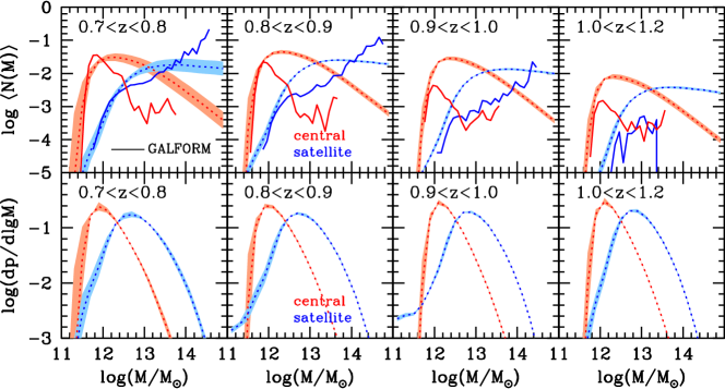
Figure 11.— Halo occupation distribution functions for the central (red dotted lines) and satellite galaxies (blue dotted lines). The shaded area are the 1$\sigma$ distribution. For comparison, the predictions from the SAM of GALFORM are shown as the red and blue solid lines for central and satellite galaxies, respectively.

We show the best-fitting halo occupation distribution function $\langle N(M)\rangle$ for the observed ELGs in different redshift bins in the top panels of Figure 11. The central and satellite galaxies are shown with red dotted lines and blue dotted lines, respectively. The shaded area represents the 1$\sigma$ error distribution. The occupation functions differ from the standard HOD form of Zheng et al. (2007) with the significant decrease of occupation numbers at the massive end (see also Geach et al., 2012; Contreras et al., 2013). Because we are only including the star-forming galaxies that have additional dependence on the quenched fraction $f_{\rm q}(M)$, the massive halos are dominated by the red/quiescent central galaxies. In our best-fitting models, the satellite occupation functions become flat at the massive end, due to the lack of star-forming satellite galaxies in very massive halos.

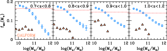
Figure 12.— Satellite galaxy fraction $f_{\rm sat}(M_{*})$ (open circles) from the best-fitting models. The average satellite fraction $\langle f_{\rm sat}\rangle$ of each sample is displayed as the red dotted line. The model predictions of the SAM of GALFORM are shown as the filled triangles.

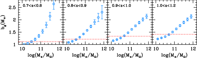
Figure 13.— Similar to Figure 12, but for the galaxy bias parameter.

We also compare our best-fitting models to the predictions from the semi-analytical model (SAM) of GALFORM with updated model treatments of Gonzalez-Perez et al. (2018) (hereafter GP18) as described in Griffin et al. (2018) (also V. Gonzalez-Perez et al., in prep.), which are shown as the red and blue solid lines for central and satellite galaxies, respectively. The galaxies from the SAM of GP18 were selected using flux, magnitude and color cuts to mimic the eBOSS ELG target sample from Raichoor et al. (2017). Our predictions show good agreement with GP18 for the low-mass cutoff profiles, i.e., the ELGs usually live in halos more massive than $10^{11.4}M_{\sun}$. It sets the requirement of the simulation resolution to generate the mock galaxy samples for the observed ELGs (see e.g., Chuang et al., 2015; Lippich et al., 2019). However, the central galaxy occupation functions of GP18 are significantly smaller than our model predictions for massive halos, which may be due to the treatment of the dust attenuation for the most massive star-forming galaxies in the SAM (Gonzalez-Perez et al., 2018).

We also note that the predicted number densities of the [O II] emitters in the GALFORM model are significantly smaller than the observed ones in the eBOSS sample at $z>0.8$ (see Figure 5 of Gonzalez-Perez et al., 2018). Moreover, the satellite fraction for the ELGs in the GP18 model is only around 5%, implying that the star formation in the satellite galaxies is suppressed too effectively. Interestingly, the discrepancies of the satellite occupation numbers in massive halos could possibly be related to the problem of the merger-driven formation model for massive galaxies. As shown in recent studies (e.g. Lapi et al., 2018b), the in-situ processes may be more relevant in driving the stellar and black hole mass growth. While our modeling results provide useful constraints to the ELGs in the SAMs, detailed comparisons to the SAMs is beyond the scope of this work.

We show in the bottom panels of Figure 11 the normalized probability distributions of the host halo masses of the central (red lines) and satellite (blue lines) ELGs, which are generated from the product of the occupation function and the differential halo mass function (Zheng et al., 2009; Guo et al., 2014). The peak halo mass distribution of the central ELGs is around $10^{12}M_{\sun}$, while the satellite galaxies live in more massive halos of $10^{12.7}M_{\sun}$. There is only a weak trend in the evolution of the halo mass distribution at $0.7<z<1.2$, consistent with the trend in the predicted SHMRs of Figure 7.

Although our best-fitting models of the occupation functions have small scatters, it is related to the fact that we have assumed a specific functional form of $f_{\rm q}(M)$. We note that the exact shape of the occupation function at the massive end is slightly dependent on the functional form of $f_{\rm q}(M)$, as will be discussed in the Appendix. However, the detailed high-mass end shape of the occupation function does not affect our constraints on the host halo mass distributions of the ELGs, as the halo mass function decreases very fast toward the massive end.

4.3.3 Satellite Galaxy Fraction

We show the satellite galaxy fraction in the observed ELG samples as the open circles in Figure 12, where the model predictions from the SAM of GALFORM are shown as the filled triangles. The average satellite fraction $\langle f_{\rm sat}\rangle$ of each sample is displayed as the red dotted line. The average satellite fraction varies from about 13% to 17%, with the higher redshift samples having slightly smaller $f_{\rm sat}$. The satellite fraction $f_{\rm sat}(M_{*})$ is generally decreasing with the stellar mass. The SAM of GALFORM generally underestimates the satellite fraction of the ELGs at different stellar masses. Since the majority of the observed ELGs are central galaxies, the discrepancies of the satellite occupation functions between our models and those of GALFORM in Figure 11 would not have a significant effect on the predicted sample number densities.

Favole et al. (2016) found a satellite fraction of around $22\%$ for a g-band selected galaxy sample in $0.6<z<1$ using a modified subhalo abundance matching model to include the incompleteness effect. Their result is slightly larger than our estimates, but the detailed value of the satellite fraction is sample-dependent, as their photometrically selected sample may include more satellite galaxies.

4.3.4 Galaxy Bias

The galaxy bias $b_{\rm g}(M_{*})$ is shown as the filled circles in Figure 13, where the average galaxy bias $\langle b_{\rm g}\rangle$ is also displayed as the dotted lines. The galaxy bias is apparently a strongly increasing function of the galaxy stellar mass, varying from $1$ to $3$. The average galaxy bias $\langle b_{\rm g}\rangle$ increases from $1.1$ at $z\sim 0.7$ to $1.4$ at $z\sim 1.2$. It is also consistent with the fact that the majority of the central ELGs in these redshift ranges live in halos of $\sim 10^{12}M_{\sun}$ that have similar halo bias values.

5. Discussions

The ICSMF model is a powerful method to simultaneously constrain the stellar mass completeness and the SHMR for current and future surveys. The constraining power of the method comes from the accurate measurements of the observed SMFs and galaxy 2PCFs, which rely on the large sample volumes of the galaxy surveys. As shown in the previous section and discussed in G18, the final model constraints are relatively independent of the detailed functional forms of the ICSMF model ingredients, once they are flexible enough to account for the selection effects in the real galaxy survey data.

Different from the many previous deep galaxy surveys with photometric redshifts, the eBOSS ELG survey has obtained accurate redshift information for most of the observed galaxies. By modeling the ELG samples at different redshift intervals independently, we can reliably study the evolution of the star-forming galaxies without assuming any redshift dependency in the model parameters, which may distort the high-redshift results in order to fit the low-redshift measurements. However, limited by the low completeness of the eBOSS ELG sample, the clustering measurements at these redshifts are still noisy. The resulting constraints on the SHMRs and intrinsic SMFs are not as accurate as those at low redshifts with volume-limited samples (Zehavi et al., 2011; Yang et al., 2012). But the ICSMF model still provides reasonable constraints to the galaxy populations at these redshifts.

We note that in principle, the completeness of galaxy populations would depend on their stellar mass, color, and other physical properties. What we obtain in the ICSMF model should be regarded as an average sample completeness at a given stellar mass. Our current eBOSS data are not accurate enough to fully break the degeneracies. We expect the ICSMF model to provide tighter constraints in future large-scale galaxy surveys.

6. Conclusions

In this paper, we apply the ICSMF model introduced by G18 to the eBOSS ELG samples over the redshift range of $0.7<z<1.2$ for galaxies with $10^{10}M_{\sun}<M_{*}<10^{11.6}M_{\sun}$. By fitting to the observed galaxy clustering and SMF measurements, we are able to constrain the sample completeness, the SHMR and the quenched galaxy fraction at the same time, which serves as a powerful way to study galaxy evolution using the large-scale galaxy surveys. The intrinsic galaxy SMFs are then directly inferred from the ICSMF model for each galaxy sample at different redshifts.

Our main conclusions are summarized as follows.

• The average stellar mass completeness of the eBOSS ELG samples varies from 1% to 10% for different redshift samples. The galaxy samples at $z<1$ are slightly more complete, compared to the higher redshift ones.

• There is only weak evolution of the SHMR for ELGs in the redshift range of $0.7<z<1.2$ for low-mass halos of $M<10^{13}M_{\sun}$, while the high-mass end slope $\alpha$ becomes flat for $z>0.8$.

• We have obtained the intrinsic SMFs for ELGs in the four redshift bins in the range of $0.7<z<1.2$, and the SMF for total galaxies in the redshift bin of $0.7<z<0.8$.

• The low-mass end ($M_{*}<10^{11}M_{\sun}$) of the galaxy SMFs for the star-forming galaxies is roughly unchanged from $z=1.2$ to $z=0.7$.

• The peak halo mass distribution of the central ELGs is around $M\sim 10^{12}M_{\sun}$, while that of the satellite ELGs increases to $M\sim 10^{12.6}M_{\sun}$.

• The satellite fraction of the eBOSS ELG varies from $13\%$ to $17\%$ at different redshifts and the average galaxy bias increases from $1.1$ at $z\sim 0.7$ to $1.4$ at $z\sim 1.2$.

Appendix A Robustness of Model Predictions

Compared to G18, we introduce an additional quenched halo fraction $f_{\rm q}(M)$ to model the ELGs in eBOSS. Since we have assumed a simple functional form of Eq. 10 to model the variation of quenched fraction with the halo mass, it is worth checking the effect of different $f_{\rm q}(M)$ models. For comparison, we choose another $f_{\rm q}(M)$ model proposed by Zu & Mandelbaum (2016) as follows:

$$f_{\rm q}(M)=1-\exp[-(M/M_{\rm q})^{\mu}],\\$$ (A1)

where the two free parameters are $M_{\rm q}$ and $\mu$. In the following, we refer to this model as “$f_{\rm q}(M)$ model 2”, while our fiducial model is referred to as “$f_{\rm q}(M)$ model 1”.

Another potential source of uncertainty is that we have assumed the same scatter $\sigma_{*}$ in Eq. 7 for both the quiescent and star-forming galaxies. Tinker et al. (2013) had modeled the scatter $\sigma_{*}$ for the quiescent and star-forming galaxies independently using the measurements of the angular clustering and galaxy-galaxy lensing. They found a $\sigma_{*}$ value of $0.18\pm 0.05$ for quiescent galaxies and $0.25\pm 0.01$ for star-forming galaxies at $0.74<z<1$. Although we have a comparable scatter for the quiescent galaxies, our adopted scatter for the star-forming galaxies ($\sigma_{*}=0.173$ at $0.7<z<0.8$) is significantly smaller. In order to test the effect of the assumed scatter, we further include a model similar to our fiducial one, but we allow $\sigma_{*}$ for the star-forming galaxies to be a free parameter, which is referred to as “$f_{\rm q}(M)$ model 1+scatter”. In this model, we still assume a constant scatter of $\sigma_{*}=0.173$ for the quiescent galaxies.

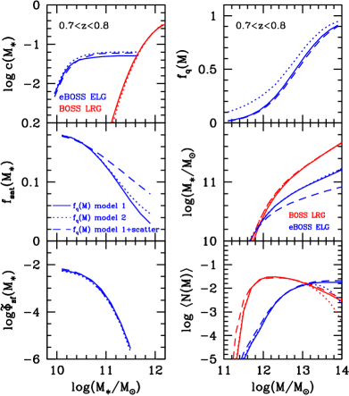
Figure 14.— Comparisons of model predictions for our fiducial model (“$f_{\rm q}(M)$ model 1”) and two variations of “$f_{\rm q}(M)$ model 2” and “$f_{\rm q}(M)$ model 1+scatter” (see text for details). The comparisons are made for the stellar mass completeness $c(M_{*})$, quenched fraction $f_{\rm q}(M)$, satellite fraction $f_{\rm sat}(M_{*})$, SHMR, intrinsic SMF $\tilde{\Phi}_{\rm sf}(M_{*})$, and the halo occupation functions $\langle N(M)\rangle$. The solid, dotted and dashed lines are for the “$f_{\rm q}(M)$ model 1”, “$f_{\rm q}(M)$ model 2” and “$f_{\rm q}(M)$ model 1+scatter”, respectively.

We show in Figure 14 the comparisons of best fits from the above three models using the BOSS LRG and eBOSS ELG measurements at $0.7<z<0.8$. The comparisons are made for the stellar mass completeness $c(M_{*})$, quenched fraction $f_{\rm q}(M)$, satellite fraction $f_{\rm sat}(M_{*})$, SHMR, intrinsic galaxy SMF of $\tilde{\Phi}_{\rm sf}(M_{*})$, and the halo occupation functions as in previous figures. The solid, dotted and dashed lines are for the “$f_{\rm q}(M)$ model 1”, “$f_{\rm q}(M)$ model 2” and “$f_{\rm q}(M)$ model 1+scatter”, respectively.

The best-fitting $\sigma_{*}$ for the “$f_{\rm q}(M)$ model 1+scatter” is $\sigma_{*}=0.22^{+0.05}_{-0.04}$, basically consistent with our model assumption within the errors. The scatter is not tightly constrained with the current eBOSS ELG sample due to the noisy clustering measurements. The inclusion of $\sigma_{*}$ as a free parameter makes the high-mass end slope of the SHMR shallower, which increases the satellite fraction at the massive end, as galaxies at a given stellar mass would have higher chances to populate the massive halos. However, other model predictions stay roughly the same with a larger $\sigma_{*}$.

Adopting the “$f_{\rm q}(M)$ model 2” would affect the quenched fraction at the $\sim 10\%$ level, with more halos hosting quenched central galaxies, especially for low-mass halos. However, as the constrained stellar mass completeness is relatively higher in order to fit the observed SMF of $\Phi_{\rm sf}(M_{*})$, the final intrinsic SMF $\tilde{\Phi}_{\rm sf}(M_{*})$ of the different models still have very good agreement with each other. As discussed previously, the exact high-mass end slopes of the halo occupation functions for both central and satellite galaxies would depend on the detailed model choice of $f_{\rm q}(M)$, while the differences at the low-mass end are relatively small. As the most massive halos only have minor contributions to the overall halo mass function, the average host halo mass distributions are consistent among different models. The SHMR of “$f_{\rm q}(M)$ model 2” is still in reasonable agreement with our fiducial model.

In addition, although we have applied a constant $M_{\rm q}$ value constrained from $0.7<z<0.8$ to higher redshift bins, our model constraints at these redshifts stay roughly the same for varying $M_{\rm q}$ values within the 1$\sigma$ range of $12.83\pm 0.24$, similar to the situation with changing the $f_{\rm q}(M)$ models. While the SHMR can be constrained by the clustering measurements, changing the $f_{\rm q}(M)$ will be compensated by the corresponding changes in the stellar mass completeness functions as shown in Eqs. (12)–(21).

References

- Bates et al. (2018) Bates, D., Tojeiro, R., Newman, J. A., et al. 2018, arXiv:1810.01767
- Behroozi et al. (2010) Behroozi, P. S., Conroy, C., & Wechsler, R. H. 2010, ApJ, 717, 379
- Behroozi et al. (2013a) Behroozi, P. S., Wechsler, R. H., & Conroy, C. 2013a, ApJ, 770, 57
- Behroozi et al. (2013b) Behroozi, P. S., Wechsler, R. H., & Wu, H.-Y. 2013b, ApJ, 762, 109
- Bernardi et al. (2016) Bernardi, M., Meert, A., Sheth, R. K., et al. 2016, MNRAS, 455, 4122
- Beutler et al. (2013) Beutler, F., Blake, C., Colless, M., et al. 2013, MNRAS, 429, 3604
- Blanton et al. (2017) Blanton, M. R., Bershady, M. A., Abolfathi, B., & et al. 2017, AJ, 154, 28
- Bruzual & Charlot (2003) Bruzual, G., & Charlot, S. 2003, MNRAS, 344, 1000
- Chabrier (2003) Chabrier, G. 2003, PASP, 115, 763
- Charlot & Fall (2000) Charlot, S., & Fall, S. M. 2000, ApJ, 539, 718
- Chuang et al. (2015) Chuang, C.-H., Zhao, C., Prada, F., et al. 2015, MNRAS, 452, 686
- Colless (1999) Colless, M. 1999, Philosophical Transactions of the Royal Society of London Series A, 357, 105
- Comparat et al. (2017a) Comparat, J., Prada, F., Yepes, G., & Klypin, A. 2017a, MNRAS, 469, 4157
- Comparat et al. (2016a) Comparat, J., Delubac, T., Jouvel, S., et al. 2016a, A&A, 592, A121
- Comparat et al. (2016b) Comparat, J., Zhu, G., Gonzalez-Perez, V., et al. 2016b, MNRAS, 461, 1076
- Comparat et al. (2017b) Comparat, J., Maraston, C., Goddard, D., et al. 2017b, arXiv:1711.06575
- Contreras et al. (2013) Contreras, S., Baugh, C. M., Norberg, P., & Padilla, N. 2013, MNRAS, 432, 2717
- Coupon et al. (2015) Coupon, J., Arnouts, S., van Waerbeke, L., et al. 2015, MNRAS, 449, 1352
- Davidzon et al. (2017) Davidzon, I., Ilbert, O., Laigle, C., et al. 2017, A&A, 605, A70
- Davis & Peebles (1983) Davis, M., & Peebles, P. J. E. 1983, ApJ, 267, 465
- Dawson et al. (2013) Dawson, K. S., Schlegel, D. J., Ahn, C. P., et al. 2013, AJ, 145, 10
- Dawson et al. (2016) Dawson, K. S., Kneib, J.-P., Percival, W. J., et al. 2016, AJ, 151, 44
- de Jong et al. (2016) de Jong, R. S., Barden, S. C., Bellido-Tirado, O., et al. 2016, in Proc. SPIE, Vol. 9908, Ground-based and Airborne Instrumentation for Astronomy VI, 99081O
- Delubac et al. (2017) Delubac, T., Raichoor, A., Comparat, J., et al. 2017, MNRAS, 465, 1831
- DESI Collaboration et al. (2016) DESI Collaboration, Aghamousa, A., Aguilar, J., & et al. 2016, arXiv:1611.00036
- Drinkwater et al. (2018) Drinkwater, M. J., Byrne, Z. J., Blake, C., et al. 2018, MNRAS, 474, 4151
- Favole et al. (2016) Favole, G., Comparat, J., Prada, F., et al. 2016, MNRAS, 461, 3421
- Geach et al. (2012) Geach, J. E., Sobral, D., Hickox, R. C., et al. 2012, MNRAS, 426, 679
- Gonzalez-Perez et al. (2018) Gonzalez-Perez, V., Comparat, J., Norberg, P., et al. 2018, MNRAS, 474, 4024
- Griffin et al. (2018) Griffin, A. J., Lacey, C. G., Gonzalez-Perez, V., et al. 2018, arXiv:1806.08370
- Gunn et al. (2006) Gunn, J. E., Siegmund, W. A., Mannery, E. J., et al. 2006, AJ, 131, 2332
- Guo et al. (2018) Guo, H., Yang, X., & Lu, Y. 2018, ApJ, 858, 30
- Guo et al. (2013) Guo, H., Zehavi, I., Zheng, Z., et al. 2013, ApJ, 767, 122
- Guo et al. (2014) Guo, H., Zheng, Z., Zehavi, I., et al. 2014, MNRAS, 441, 2398
- Hill et al. (2008) Hill, G. J., Gebhardt, K., Komatsu, E., et al. 2008, in Astronomical Society of the Pacific Conference Series, Vol. 399, Panoramic Views of Galaxy Formation and Evolution, ed. T. Kodama, T. Yamada, & K. Aoki, 115
- Hudson et al. (2015) Hudson, M. J., Gillis, B. R., Coupon, J., et al. 2015, MNRAS, 447, 298
- Ilbert et al. (2006) Ilbert, O., Arnouts, S., McCracken, H. J., et al. 2006, A&A, 457, 841
- Ilbert et al. (2013) Ilbert, O., McCracken, H. J., Le Fèvre, O., et al. 2013, A&A, 556, A55
- Jackson (1972) Jackson, J. C. 1972, MNRAS, 156, 1P
- Kaasinen et al. (2017) Kaasinen, M., Bian, F., Groves, B., Kewley, L. J., & Gupta, A. 2017, MNRAS, 465, 3220
- Kaiser (1987) Kaiser, N. 1987, MNRAS, 227, 1
- Kennicutt (1998) Kennicutt, R. C., Jr. 1998, ApJ, 498, 541
- Kewley et al. (2004) Kewley, L. J., Geller, M. J., & Jansen, R. A. 2004, AJ, 127, 2002
- Klypin et al. (2016) Klypin, A., Yepes, G., Gottlöber, S., Prada, F., & Heß, S. 2016, MNRAS, 457, 4340
- Kriek & Conroy (2013) Kriek, M., & Conroy, C. 2013, ApJ, 775, L16
- Kriek et al. (2009) Kriek, M., van Dokkum, P. G., Labbé, I., et al. 2009, ApJ, 700, 221
- Landy & Szalay (1993) Landy, S. D., & Szalay, A. S. 1993, ApJ, 412, 64
- Lapi et al. (2017) Lapi, A., Mancuso, C., Bressan, A., & Danese, L. 2017, ApJ, 847, 13
- Lapi et al. (2018a) Lapi, A., Salucci, P., & Danese, L. 2018a, ApJ, 859, 2
- Lapi et al. (2018b) Lapi, A., Pantoni, L., Zanisi, L., et al. 2018b, ApJ, 857, 22
- Le Fèvre et al. (2013) Le Fèvre, O., Cassata, P., Cucciati, O., et al. 2013, A&A, 559, A14
- Leauthaud et al. (2016) Leauthaud, A., Bundy, K., Saito, S., et al. 2016, MNRAS, 457, 4021
- Li et al. (2006) Li, C., Kauffmann, G., Jing, Y. P., et al. 2006, MNRAS, 368, 21
- Lin et al. (2016) Lin, Y.-T., Mandelbaum, R., Huang, Y.-H., et al. 2016, ApJ, 819, 119
- Lippich et al. (2019) Lippich, M., Sánchez, A. G., Colavincenzo, M., et al. 2019, MNRAS, 482, 1786
- Mandelbaum et al. (2016) Mandelbaum, R., Wang, W., Zu, Y., et al. 2016, MNRAS, 457, 3200
- Maraston et al. (2013) Maraston, C., Pforr, J., Henriques, B. M., et al. 2013, MNRAS, 435, 2764
- Masters et al. (2011) Masters, K. L., Maraston, C., Nichol, R. C., et al. 2011, MNRAS, 418, 1055
- Mitchell et al. (2013) Mitchell, P. D., Lacey, C. G., Baugh, C. M., & Cole, S. 2013, MNRAS, 435, 87
- Montero-Dorta et al. (2016) Montero-Dorta, A. D., Bolton, A. S., Brownstein, J. R., et al. 2016, MNRAS, 461, 1131
- Moster et al. (2013) Moster, B. P., Naab, T., & White, S. D. M. 2013, MNRAS, 428, 3121
- Moustakas et al. (2013) Moustakas, J., Coil, A. L., Aird, J., et al. 2013, ApJ, 767, 50
- Muzzin et al. (2013) Muzzin, A., Marchesini, D., Stefanon, M., et al. 2013, ApJ, 777, 18
- Newman et al. (2013) Newman, J. A., Cooper, M. C., Davis, M., et al. 2013, ApJS, 208, 5
- Okada et al. (2016) Okada, H., Totani, T., Tonegawa, M., et al. 2016, PASJ, 68, 47
- Orsi et al. (2014) Orsi, Á., Padilla, N., Groves, B., et al. 2014, MNRAS, 443, 799
- Peng et al. (2012) Peng, Y.-j., Lilly, S. J., Renzini, A., & Carollo, M. 2012, ApJ, 757, 4
- Pérez-González et al. (2008) Pérez-González, P. G., Rieke, G. H., Villar, V., et al. 2008, ApJ, 675, 234
- Planck Collaboration et al. (2014) Planck Collaboration, Ade, P. A. R., Aghanim, N., & et al. 2014, A&A, 571, A16
- Raichoor et al. (2016) Raichoor, A., Comparat, J., Delubac, T., et al. 2016, A&A, 585, A50
- Raichoor et al. (2017) Raichoor, A., Comparat, J., Delubac, T., et al. 2017, MNRAS, 471, 3955
- Reid et al. (2016) Reid, B., Ho, S., Padmanabhan, N., et al. 2016, MNRAS, 455, 1553
- Rodríguez-Puebla et al. (2015) Rodríguez-Puebla, A., Avila-Reese, V., Yang, X., et al. 2015, ApJ, 799, 130
- Rodríguez-Puebla et al. (2017) Rodríguez-Puebla, A., Primack, J. R., Avila-Reese, V., & Faber, S. M. 2017, MNRAS, 470, 651
- Saito et al. (2016) Saito, S., Leauthaud, A., Hearin, A. P., et al. 2016, MNRAS, 460, 1457
- Schechter (1976) Schechter, P. 1976, ApJ, 203, 297
- Shankar et al. (2014) Shankar, F., Guo, H., Bouillot, V., et al. 2014, ApJ, 797, L27
- Takada et al. (2014) Takada, M., Ellis, R. S., Chiba, M., et al. 2014, PASJ, 66, R1
- Tinker et al. (2013) Tinker, J. L., Leauthaud, A., Bundy, K., et al. 2013, ApJ, 778, 93
- Tinker et al. (2010) Tinker, J. L., Robertson, B. E., Kravtsov, A. V., et al. 2010, ApJ, 724, 878
- Tinker et al. (2017) Tinker, J. L., Brownstein, J. R., Guo, H., et al. 2017, ApJ, 839, 121
- Tomczak et al. (2014) Tomczak, A. R., Quadri, R. F., Tran, K.-V. H., et al. 2014, ApJ, 783, 85
- van den Bosch et al. (2013) van den Bosch, F. C., More, S., Cacciato, M., Mo, H., & Yang, X. 2013, MNRAS, 430, 725
- Wang & Jing (2010) Wang, L., & Jing, Y. P. 2010, MNRAS, 402, 1796
- Wechsler & Tinker (2018) Wechsler, R. H., & Tinker, J. L. 2018, ARA&A, 56, 435
- Wright et al. (2010) Wright, E. L., Eisenhardt, P. R. M., Mainzer, A. K., et al. 2010, AJ, 140, 1868
- Yang et al. (2009) Yang, X., Mo, H. J., & van den Bosch, F. C. 2009, ApJ, 695, 900
- Yang et al. (2013) Yang, X., Mo, H. J., van den Bosch, F. C., et al. 2013, ApJ, 770, 115
- Yang et al. (2012) Yang, X., Mo, H. J., van den Bosch, F. C., Zhang, Y., & Han, J. 2012, ApJ, 752, 41
- York et al. (2000) York, D. G., Adelman, J., Anderson, Jr., J. E., et al. 2000, AJ, 120, 1579
- Zehavi et al. (2011) Zehavi, I., Zheng, Z., Weinberg, D. H., et al. 2011, ApJ, 736, 59
- Zhao et al. (2016) Zhao, G.-B., Wang, Y., Ross, A. J., et al. 2016, MNRAS, 457, 2377
- Zheng et al. (2007) Zheng, Z., Coil, A. L., & Zehavi, I. 2007, ApJ, 667, 760
- Zheng & Guo (2016) Zheng, Z., & Guo, H. 2016, MNRAS, 458, 4015
- Zheng et al. (2009) Zheng, Z., Zehavi, I., Eisenstein, D. J., Weinberg, D. H., & Jing, Y. P. 2009, ApJ, 707, 554
- Zheng et al. (2005) Zheng, Z., Berlind, A. A., Weinberg, D. H., et al. 2005, ApJ, 633, 791
- Zhu et al. (2015) Zhu, G. B., Comparat, J., Kneib, J.-P., et al. 2015, ApJ, 815, 48
- Zu & Mandelbaum (2016) Zu, Y., & Mandelbaum, R. 2016, MNRAS, 457, 4360