Second Order Linear Energy Stable Schemes for Allen-Cahn Equations with Nonlocal Constraints

Abstract

We present a set of linear, second order, unconditionally energy stable schemes for the Allen-Cahn equation with nonlocal constraints that preserves the total volume of each phase in a binary material system. The energy quadratization strategy is employed to derive the energy stable semi-discrete numerical algorithms in time. Solvability conditions are then established for the linear systems resulting from the semi-discrete, linear schemes. The fully discrete schemes are obtained afterwards by applying second order finite difference methods on cell-centered grids in space. The performance of the schemes are assessed against two benchmark numerical examples, in which dynamics obtained using the volume-preserving Allen-Cahn equations with nonlocal constraints is compared with those obtained using the classical Allen-Cahn as well as the Cahn-Hilliard model, respectively, demonstrating slower dynamics when volume constraints are imposed as well as their usefulness as alternatives to the Cahn-Hilliard equation in describing phase evolutionary dynamics for immiscible material systems while preserving the phase volumes. Some performance enhancing, practical implementation methods for the linear energy stable schemes are discussed in the end.

Keywords: Phase field model, energy stable schemes, energy quadratization, nonlocal constraints, volume preserving.

1 Introduction

Thermodynamically consistent models for material systems represent a class of models that yield the energy dissipation law. One particular class of the models is known as the gradient flow, in which the time evolution of thermodynamical variables is proportional to the variation of the system free energy. When the thermodynamic variable is a phase variable, it’s known as the Allen-Cahn equation. This class of models describes relaxation dynamics of the thermodynamical system to equilibrium. There are many applications of such gradient flow equations, particularly in the materials science, life science and fluid dynamics [1, 4, 17, 8, 17, 19, 15, 23, 14, 32, 36, 37, 30, 34, 7, 16]. However, in the case of a phase field description, when the phase variable represents the volume fraction of a material component, this model does not warrant the conservation of the volume of that component. In order to preserve the volume, the free energy functional has to be augmented by a volume preserving mechanism with a penalizing potential term or a Lagrange multiplier [20][24]. This often results in a nonlocal term in the modified Allen-Cahn equation. In this paper, we call these nonlocal Allen-Cahn equations or Allen-Cahn equations with nonlocal constraints.

The Cahn-Hilliard equation is an alternative model for the gradient flow. One feature of the Cahn-Hilliard equation is its volume preserving property. Rubinstein and Sternberg studied the Allen-Cahn model with the volume constraint analytically and compared it with the Cahn-Hilliard model [24]. Their result favors using the Allen-Cahn model with a volume constraint in place of the Cahn-Hilliard model when studying interfacial dynamics of incompressible, immiscible multi-component material systems. For the Allen-Cahn equation as well as the Cahn-Hilliard equation, there have been several popular numerical approaches to construct energy stable schemes for the equations, including the convex splitting approach [11, 13, 12, 30, 25, 28, 18] , the stabilizing approach [27, 10, 6], the energy quadratization (EQ) approach [39, 33, 15, 14] and the scalar auxiliary variable approach, which is a special form of EQ method, [26, 9, 29]. Recently, the energy quadratization (EQ) and its reincarnation in the scalar auxiliary variable (SAV) method have been applied to a host of thermodynamical and hydrodynamic models owing to their simplicity, ease of implementation, computational efficiency, linearity, and most importantly their energy stability property [35, 33, 15, 14, 32, 36, 37, 5, 31, 40, 38, 41, 9, 29]. We have shown that these strategies are general enough to be useful for developing energy stable numerical approximations to any thermodynamically consistent models, i.e., the models derived using the second law of thermodynamics or the Onsager principle [21, 22, 39].

In this paper, we develop a set of linear, second order, unconditionally energy stable schemes using the energy quadratization (EQ) and scalar auxiliary variable (SAV) approach to solve the Allen-Cahn equation, nonlocal Allen-Cahn equation and Cahn-Hilliard equations numerically. The numerical schemes for the Allen-Cahn and the Cahn-Hilliard model are not new. They are presented here for comparison purposes. However, the schemes for the nonlocal Allen-Cahn models are new. In some of these schemes, both EQ and SAV approaches are combined to yield linear, energy stable schemes. We note that when a nonlocal Allen-Cahn model is discretized, it is inevitable to yield an SAV scheme when the EQ strategy is applied. When multiple integrals are identified as SAVs in the free energy functional, new iterative steps are proposed to solve the subproblems in which elliptic equations are solved efficiently. All these schemes are linear and second order accurate in time. The linear system resulting from the schemes are all solvable uniquely so that the solution existence and uniqueness in the semi-discrete system is warranted. When EQ is coupled with the discretized integrals, the Sherman-Morrison formula can lead us to an efficient numerical scheme. This can be equivalently be dealt with using the SAV method as well. The numerical schemes developed for the Allen-Cahn equation with nonlocal volume-preserving constraints also preserves the volume at the discrete level in addition to preserving the energy dissipation rate. In the end, we conduct two numerical experiments to assess the performance of the schemes. The results based on EQ and those based on SAV perform equally well in preserving the volume and energy dissipation rate. In addition, the computational efficiency of the schemes is comparatively studied in one of the benchmark examples. Some performance enhancing, practical implementation methods are discussed to improve the accuracy of the schemes at large time step sizes. To simplify our presentation, we present the temporal discretization of the models using EQ and SAV approaches in detail. Then, we briefly discuss our strategy to obtain fully discrete schemes by discretizing the semi-discrete schemes in space, and refer readers to our early publications in [15, 14] for more details.

The rest of paper is organized as follows. In $\S 2$, we present the mathematical models for the Allen-Cahn, the Allen-Cahn with nonlocal constraints, and the Cahn-Hilliard equation. In $\S 3$, we study their near equilibrium dynamics. In $\S 4$, we present a set of second order, linear, energy stable numerical schemes for the models. In $\S 5$, we conduct mesh refinement tests on all the schemes and carry out two simulations on drop merging as well as phase coarsening experiments using the models. Finally, we give the concluding remark in section $\S 6$.

2 Phase Field Models for Binary Materials

We briefly review two simple phase field models for a binary material system: the Allen-Cahn and the Cahn-Hilliard model, in which the free energy density of the binary material system is given by a functional of phase variable $\phi\in[0,1]$ and its gradients. For instance, to study drops of one fluid within the matrix of the other immiscible fluid while ignoring hydrodynamic effects, the free energy is customarily chosen as the following double-well potential:

$$\begin{array}[]{l}F=\int_{\Omega}\gamma[\frac{\epsilon}{2}{(\nabla\phi)}^{2}+\frac{1}{\epsilon}\phi^{2}(1-\phi)^{2}]\mathrm{d{\bf r}},\end{array}$$ (2.2)

where $\Omega$ is the material domain, $\epsilon$ is a parameter describing the width of the interface and $\gamma$ is proportional to the surface tension. In general, the generic form of some commonly used free energies are given as follows

$$\begin{array}[]{l}F=\int_{\Omega}[\gamma_{1}{(\nabla\phi)}^{2}+f(\phi)]\mathrm{d{\bf r}},\end{array}$$ (2.4)

where $\gamma_{1}$ parametrizes the conformational entropy and $f(\phi)$ is the bulk potential.

Dynamics of the binary material system is customarily governed by a time dependent partial differential equation model resulting from the Onsager’s linear response theory[21, 22],

$$\begin{array}[]{l}\frac{\partial\phi}{\partial t}=-M\mu,in\;\Omega,\\ \mu=\frac{\delta F}{\delta\phi}=-2\gamma_{1}\nabla^{2}\phi+f^{\prime}(\phi),\end{array}$$ (2.7)

subject to appropriate boundary and initial conditions, where $M$ is the mobility matrix consisting of differential operators of even order and $\mu$ is the chemical potential.

The time rate of change of the free energy, known as the energy dissipation functional, is given by

$$\frac{dF}{dt}=-\int_{\Omega}\mu M\mu\mathrm{d{\bf r}}+\int_{\partial\Omega}{\bf n}\cdot\frac{\partial f}{\partial\nabla\phi}\phi_{t}ds.$$ (2.8)

The no-flux boundary condition

$${\bf n}\cdot\frac{\partial f}{\partial\nabla\phi}=0$$ (2.9)

annihilates the energy dissipation at the boundary, where $\bf n$ is the unit external normal of the boundary. This is the commonly used boundary condition. Another less-used boundary condition is

$$\phi_{t}=-\beta{\bf n}\cdot\frac{\partial f}{\partial\nabla\phi}.$$ (2.10)

This specifies a decay rate of the phase variable at the boundary for $\beta\geq 0$.

The system is dissipative with respect to both boundary conditions provided $M$ is a positive definite operator. The commonly used phase field models such as Allen-Cahn and Cahn-Hilliard are two special cases, corresponding to

$$M=\left\{\begin{array}[]{ll}M_{0},&\hbox{Allen-Cahn},\\ -\nabla\cdot M_{0}\nabla,&\hbox{Cahn-Hilliard},\end{array}\right.$$ (2.13)

respectively, where $M_{0}$ is a prescribed mobility coefficient matrix, which is a function of $\phi$. However, in some case, a constant mobility is used as an approximation instead. The Allen-Cahn equation defined this way does not conserve the total volume $\int_{\Omega}\phi\mathrm{d\mathbf{r}}$ if $\phi$ is the volume-fraction while the Cahn-Hilliard equation does. However, these two models predict similar near equilibrium dynamics revealed in their linear stability analyses below. On the other hand, the Allen-Cahn equation is an equation of lower spatial derivatives, and presumably costs less when solved numerically. Thus, one opted to impose the volume conservation as a constraint to the Allen-Cahn equation for it to be able to describe dynamics in which the volume is conserved in some cases. Next, we will briefly recall several ways to impose volume conservation to dynamics described by the Allen-Cahn equation, then discuss how to design efficient and energy stable numerical algorithms to compute their numerical solutions.

2.1 Allen-Cahn model

The Allen-Cahn equation with the no-flux Neumann boundary condition and initial conditions is given as follows:

$$\begin{array}[]{l}\frac{\partial\phi}{\partial t}=-M\mu,in\;\Omega\\ \frac{\partial\phi}{\partial n}=0,in\;\partial\Omega,\\ \phi|_{t=0}=\phi(\mathbf{r},0),\mathbf{r}\;in\;\Omega.\end{array}$$ (2.17)

The energy dissipation rate of the Allen-Cahn equation is given by (2.8) We denote the volume of $\Omega$ by

$$V(t)=\int_{\Omega}\phi\mathrm{d{\bf r}}.$$ (2.18)

Then,

$$\frac{dV}{dt}=-\int_{\Omega}M\mu\mathrm{d{\bf r}}.$$ (2.19)

It is normally nonzero provided $M\neq 0$, which implies that $V(t)$ is not conserved. One simple fix is to enforce the volume constraint $V(t)=V(0)$ by coupling it to the Allen-Cahn dynamical equation. The resulting equation is termed the Allen-Cahn equation with nonlocal constraints.

2.2 Allen-Cahn models with nonlocal constraints

In addition to the approximate volume defined above, $V(t)=\int_{\Omega}\phi(t)\mathrm{d{\bf r}}$, we can introduce a more general definition using a function $h(\phi)$, which is (i) monotonically increasing for $\phi\in[0,1]$, and (ii) $h(0)=0,h(1)=1$ as follows,

$$V(t)=\int_{\Omega}h(\phi)d\mathbf{r}.$$ (2.20)

We next discuss methods to enforce volume conservation for the Allen-Cahn model. First, we consider the method that minimizes $(V(t)-V(0))^{2}$ by penalizing it in the free energy functional.

2.2.1 Allen-Cahn model with a penalizing potential

Here, we augment the free energy with a penalizing potential term as follows

$$\begin{array}[]{l}F=\int_{\Omega}[\gamma_{1}{(\nabla\phi)}^{2}+f(\phi)]\mathrm{d{\bf r}}+\frac{\eta}{2}(V(t)-V(0))^{2},\end{array}$$ (2.22)

where $\eta$ is the penalizing parameter, a large positive constant. The transport equation for $\phi$ is given by the Allen-Cahn equation with the modified chemical potential

$$\begin{array}[]{l}\tilde{\mu}=\frac{\delta F}{\delta\phi}=\mu+\sqrt{\eta}\zeta h^{\prime}(\phi),\quad\zeta=\sqrt{\eta}(V(t)-V(0)).\end{array}$$ (2.24)

The energy dissipation rate is given by

$$\begin{array}[]{l}\frac{dF}{dt}=\int_{\Omega}\frac{\delta F}{\delta\phi}\phi_{t}\mathrm{d{\bf r}}=-\int_{\Omega}\tilde{\mu}(M\tilde{\mu})\mathrm{d{\bf r}}.\end{array}$$ (2.26)

It is negative if $M\geq 0$. The modified Allen-Cahn equation is approximately volume-conserving depending on the size of $\eta$. In principle, an appropriate $\eta>0$ can make $V(t)$ close to $V(0)$. The choice of $\eta$ is, however, up to the user.

2.2.2 Allen-Cahn models with a Lagrange multiplier

To enforce the volume conservation in the Allen-Cahn model exactly, we use a Lagrange multiplier $L$ for constraint $V(t)-V(0)=0$. This can be accomplished by augmenting a penalty term with a Lagrange multiplier $L$ in the free energy functional as follows:

$$\tilde{F}=F-L(V(t)-V_{0}).$$ (2.27)

The transport equation for $\phi$ is given by the Allen-Cahn equation with a modified chemical potential $\tilde{\mu}$ given by

$$\begin{array}[]{l}\tilde{\mu}=\frac{\delta F}{\delta\phi}=\mu-Lh^{\prime}(\phi),\end{array}$$ (2.29)

where $h^{\prime}(\phi)=\frac{\delta h(\phi)}{\delta\phi}$ and $V(t)-V(0)=0$ is enforced. Since the volume is conserved,

$$\int_{\Omega}[h^{\prime}(\phi)\frac{d\phi}{dt}]\mathrm{d{\bf r}}=\int_{\Omega}[h^{\prime}(\phi)M\tilde{\mu}]\mathrm{d{\bf r}}=0.$$ (2.30)

We arrive at

$$\begin{array}[]{l}L=\frac{1}{\int_{\Omega}h^{\prime}(\phi)Mh^{\prime}(\phi)\mathrm{d{\bf r}}}\int_{\Omega}[h^{\prime}(\phi)M\mu]\mathrm{d{\bf r}}.\end{array}$$ (2.32)

The volume conserved Allen-Cahn equation is nonlocal because an integral is in the chemical potential as well as in the equation. The choice of $h(\phi)$ in this paper includes the following two families.

$$\left\{\begin{array}[]{l}h(\phi)=\phi,\\ h^{\prime}(\phi)=\frac{(m+1)(2m+1)}{m}[\phi(1-\phi)]^{m},m\hbox{ is a positive integer}.\end{array}\right.$$ (2.35)

The energy dissipation is again given by (2.26).

2.3 Cahn-Hilliard model

In the Cahn-Hilliard model, the transport equation for $\phi$ is given by

$$\begin{array}[]{l}\frac{\partial\phi}{\partial t}=\nabla\cdot(M\nabla\mu),in\;\Omega\\ \frac{\partial\phi}{\partial n}=0,\frac{\partial\mu}{\partial n}=0,in\;\partial\Omega\\ \phi|_{t=0}=\phi(\mathbf{r},0).\end{array}$$ (2.39)

The energy dissipation rate of the Cahn-Hilliard equation is given by

$$\begin{array}[]{l}\frac{dF}{dt}=\int_{\Omega}\frac{\delta F}{\delta\phi}\phi_{t}\mathrm{d{\bf r}}=-\int_{\Omega}(\nabla\mu)M(\nabla\mu)\mathrm{d{\bf r}}\leq 0,\end{array}$$ (2.41)

provided $M$ is nonnegative definite. We next compare the near equilibrium dynamics of the modified Allen-Cahn equations and the Cahn-Hilliard equation.

3 Near equilibrium dynamics

We conduct a linear stability analysis about a constant steady state in a rectangular domain to investigate near equilibrium dynamics of the phase field models mentioned above. Specifically, we perturb the steady state $\phi^{ss}$ of the equations by a small disturbance $\delta v$,

$$\begin{array}[]{l}\phi=\phi^{ss}+\delta v.\end{array}$$ (3.2)

For the Allen-Cahn model, substituting equation (3.2) into equation (2.17), we get the linearized equation

$$\begin{array}[]{l}\frac{\partial\delta v}{\partial t}=-M[-2\gamma_{1}\nabla^{2}\delta v+f^{\prime\prime}(\phi^{ss})\delta v].\end{array}$$ (3.4)

We solve it using the Fourier series method in domain $\Omega=[-\pi,\pi]^{2}$ with $\delta v=\sum_{k,l=0}^{\infty}a_{kl}(t)cos(kx)cos(ly)$ that satisfies the boundary condition. Then we obtain the following ordinary differential equation system for each single mode

$$\begin{array}[]{l}\dot{a}_{kl}(t)=-Ma_{kl}(t)[2\gamma_{1}(k^{2}+l^{2})+f^{\prime\prime}(\phi^{ss})],k,l=0,\cdots,\infty.\end{array}$$ (3.6)

In this system, instability may occur only if $f^{\prime\prime}(\phi^{ss})<0$ and $2\gamma_{1}(k^{2}+l^{2})+f^{\prime\prime}(\phi^{ss})<0$ for some small $k,l$.

For the Allen-Cahn model with a penalizing potential, substituting equation (3.2) into the transport equation, we get the linearized equation

$$\begin{array}[]{l}\frac{\partial\delta v}{\partial t}=-M(-2\gamma_{1}\nabla^{2}\delta v+f^{\prime\prime}(\phi^{ss})\delta v+\eta[h^{\prime\prime}(\phi^{ss})\delta v(\int_{\Omega}h(\phi^{ss})\mathrm{d{\bf r}}-V(0))+h^{\prime}(\phi^{ss})\int_{\Omega}h^{\prime}(\phi^{ss})\delta v\mathrm{d{\bf r}}]).\end{array}$$ (3.8)

We solve it analogously and obtain governing system of equations for the Fourier coefficients:

$$\begin{array}[]{l}\dot{a}_{kl}(t)=-Ma_{kl}(t)[2\gamma_{1}(k^{2}+l^{2})+f^{\prime\prime}(\phi^{ss})+\eta h^{\prime\prime}(\phi^{ss})(\int_{\Omega}h(\phi^{ss})\mathrm{d{\bf r}}-V(0))+\eta h^{\prime}(\phi^{ss})\int_{\Omega}h^{\prime}(\phi^{ss})\mathrm{d{\bf r}}\delta_{k0}\delta_{l0}].\end{array}$$ (3.10)

If $2\gamma_{1}(k^{2}+l^{2})+f^{\prime\prime}(\phi^{ss})+\eta h^{\prime\prime}(\phi^{ss})(\int_{\Omega}h(\phi^{ss})\mathrm{d{\bf r}}-V(0))+\eta\int_{\Omega}(h^{\prime}(\phi^{ss}))^{2}\mathrm{d{\bf r}}\delta_{k0}\delta_{l0}<0$ for some small $k,l$, instability may occur. Compared with the Allen-Cahn model, this modified Allen-Cahn introduces a stabilizing mechanism at the zero wave number $k=0$ and $l=0$ due to the average at the zero-wave number and a potentially destabilizing mechanism for $h^{\prime\prime}(\phi^{ss})<0$ and stablizing mechanism for $h^{\prime\prime}(\phi^{ss})>0$. For the simple case $h(\phi)=\phi$, the only contribution is the stabilizing mechanism at $k=0$ and $l=0.$

For the Allen-Cahn model with a Lagrangian multiplier, we denote $g(\phi)=h^{\prime}(\phi)M(-2\gamma_{1}\nabla^{2}\phi+f^{\prime}(\phi^{ss}))$. Substituting equation (3.2) into the transport equation, we get the linearized equation

$$\begin{array}[]{l}\frac{\partial\delta v}{\partial t}=-M[-2\gamma_{1}\nabla^{2}\delta v+f^{\prime\prime}(\phi^{ss})\delta v-\frac{h^{\prime\prime}(\phi^{ss})\delta v\int_{\Omega}g(\phi^{ss})\mathrm{d{\bf r}}}{\int_{\Omega}[h^{\prime}(\phi^{ss})]M[h^{\prime}(\phi^{ss})]\mathrm{d{\bf r}}}-\frac{h^{\prime}(\phi^{ss})\int_{\Omega}g^{\prime}(\phi^{ss})\delta v\mathrm{d{\bf r}}}{\int_{\Omega}[h^{\prime}(\phi^{ss})]M[h^{\prime}(\phi^{ss})]\mathrm{d{\bf r}}}+\\ 2\frac{h^{\prime}(\phi^{ss})\int_{\Omega}g(\phi^{ss})\mathrm{d{\bf r}}}{(\int_{\Omega}[h^{\prime}(\phi^{ss})]M[h^{\prime}(\phi^{ss})]\mathrm{d{\bf r}})^{2}}\int_{\Omega}[h^{\prime\prime}(\phi^{ss})]M[h^{\prime}(\phi^{ss})]\delta v\mathrm{d{\bf r}}].\end{array}$$ (3.13)

The dynamic equations for the Fourier coefficients are

$$\begin{array}[]{l}\dot{a}_{kl}(t)=-Ma_{kl}(t)[2\gamma_{1}(k^{2}+l^{2})+f^{\prime\prime}(\phi^{ss})-\frac{h^{\prime\prime}(\phi^{ss})\int_{\Omega}g(\phi^{ss})\mathrm{d{\bf r}}}{\int_{\Omega}[h^{\prime}(\phi^{ss})]M[h^{\prime}(\phi^{ss})]\mathrm{d{\bf r}}}-(\frac{h^{\prime}(\phi^{ss})\int_{\Omega}g^{\prime}(\phi^{ss})\mathrm{d{\bf r}}}{\int_{\Omega}[h^{\prime}(\phi^{ss})]M[h^{\prime}(\phi^{ss})]\mathrm{d{\bf r}}}-\\ 2\frac{h^{\prime}(\phi^{ss})\int_{\Omega}g(\phi^{ss})\mathrm{d{\bf r}}}{(\int_{\Omega}[h^{\prime}(\phi^{ss})]M[h^{\prime}(\phi^{ss})]\mathrm{d{\bf r}})^{2}}\int_{\Omega}[h^{\prime\prime}(\phi^{ss})]M[h^{\prime}(\phi^{ss})]\mathrm{d{\bf r}})\delta_{k0}\delta_{l0}].\end{array}$$ (3.16)

For the simple case $h(\phi)=\phi$,

$$\begin{array}[]{l}\dot{a}_{kl}(t)=-Ma_{kl}(t)[2\gamma_{1}(k^{2}+l^{2})+f^{\prime\prime}(\phi^{ss})-\frac{\int_{\Omega}Mf^{\prime\prime}(\phi^{ss})\mathrm{d{\bf r}}}{\int_{\Omega}M\mathrm{d{\bf r}}}\delta_{k0}\delta_{l0}].\end{array}$$ (3.18)

If $2\gamma_{1}(k^{2}+l^{2})+f^{\prime\prime}(\phi^{ss})-\frac{\int_{\Omega}Mf^{\prime\prime}(\phi^{ss})\mathrm{d{\bf r}}}{\int_{\Omega}M\mathrm{d{\bf r}}}\delta_{k0}\delta_{l0}<0$, for small $k,l$, instability may occur. Compared with the Allen-Cahn dynamics, the only contribution of the Lagrange multiplier is introducing a correction at the zero wave number limit which may be stabilizing when $f^{\prime\prime}(\phi^{ss})<0$ and destabilizing otherwise.

For the Cahn-Hilliard model, substituting equation (3.2) into equation (2.39), we get the linearized equation

$$\begin{array}[]{l}\frac{\partial\delta v}{\partial t}=M[-2\gamma_{1}\nabla^{4}\delta v+f^{\prime\prime}(\phi^{ss})\nabla^{2}\delta v)].\end{array}$$ (3.20)

Repeating the analysis, we have

$$\begin{array}[]{l}\dot{a}_{kl}(t)=-Ma_{kl}(t)[2\gamma_{1}(k^{2}+l^{2})+f^{\prime\prime}(\phi^{ss})](k^{2}+l^{2}).\end{array}$$ (3.22)

If $kl[2\gamma_{1}(k^{2}+l^{2})+f^{\prime\prime}(\phi^{ss})]<0$, instability may ensure. We note that the window of instability in the Cahn-Hilliard model is identical to that in the Allen-Cahn model. However, the rate of growth is different. These linear stability results dictate the initial transition of the solution towards or away from the steady state. For long time transient behavior of the solution, we have to resort to numerical computations.

We next discuss how to numerically approximate the model equations efficiently with high order, linear, energy stable schemes.

4 Numerical Approximations of the Phase Field Models

We design numerical schemes to solve the above nonlocal equations to ensure that the energy dissipation property as well as the total volume conservation are respected. We do it by employing the energy quadratization strategy (EQ) and the scalar auxiliary variable approach (SAV) developed recently [36, 40, 26, 31]. Both methods depend on a reformulation of the model into one with a quadratic energy, and provide effective ways to design linear numerical schemes. SAV is a specialized EQ strategy suitable for thermodynamical systems. For a full review on EQ methods on thermodynamical systems, readers are referred to a recent review article [39]. All schemes presented below are firstly semi-discretized by the Crank-Nilcolson method in time and then centrally discretized in space later. In fact, we have shown recently that BDF and Runge-Kutta methods can be used to design energy stable schemes for thermodynamical systems up to arbitrarily high order in time [35]. For simplicity, we present the schemes in their semi-discrete forms in time. For comparison purposes, we also present analogous schemes for the classical Allen-Cahn and the Cahn Hilliard model as well.

4.1 Temporal discretization

4.1.1 Numerical methods for the Allen-Cahn model using EQ

We reformulate the free energy density by introducing an intermediate variable $q$ and a constant $C_{0}>0$ such that $q$ is a real variable,

$$\begin{array}[]{l}q=\sqrt{f(\phi)-\gamma_{2}\phi^{2}+C_{0}}.\end{array}$$ (4.2)

Then, the free energy is recast into a quadratic form:

$$\begin{array}[]{l}F=\int_{\Omega}[\gamma_{1}(\nabla\phi)^{2}+\gamma_{2}\phi^{2}+q^{2}-C_{0}]\mathrm{d{\bf r}}.\end{array}$$ (4.4)

The chemical potential is give by

$$\begin{array}[]{l}\mu=\frac{\delta F}{\delta\phi}=-2\gamma_{1}\nabla^{2}\phi+2\gamma_{2}\phi+2qq^{\prime},\quad q^{\prime}=\frac{\delta q}{\delta\phi}.\end{array}$$ (4.6)

We rewrite the Allen-Cahn equation given in (2.17) using the new variables as follows

$$\begin{array}[]{l}\frac{\partial\phi}{\partial t}=-M\mu,\quad\quad\frac{\partial q}{\partial t}=q^{\prime}\phi_{t}.\end{array}$$ (4.8)

The initial condition of $q$ must be calculated from that of $\phi$. We denote

$$\begin{array}[]{l}{(\cdot)}^{n+1/2}=\frac{{(\cdot)}^{n+1}+{(\cdot)}^{n}}{2},\quad\overline{(\cdot)}^{n+1/2}=\frac{3{(\cdot)}^{n+1}-{(\cdot)}^{n}}{2}.\end{array}$$ (4.10)

A second order in time numerical algorithm is given below.

Scheme 4.1.

Given initial conditions $\phi^{0}$ and $q^{0}$ (calculated from $\phi^{0}$), we compute $\phi^{1},q^{1}$ by a first order scheme. Having computed $\phi^{n-1},q^{n-1}$, and $\phi^{n},q^{n}$, we compute $\phi^{n+1},q^{n+1}$ as follows.

$$\begin{array}[]{l}\phi^{n+1}-\phi^{n}=-\Delta t\overline{M}^{n+1/2}{\mu}^{n+1/2},\\ {\mu}^{n+1/2}=-2\gamma_{1}{\nabla^{2}\phi}^{n+1/2}+2\gamma_{2}{\phi}^{n+1/2}+2{q}^{n+1/2}\overline{q^{\prime}}^{n+1/2},\\ q^{n+1}-q^{n}=\overline{q^{\prime}}^{n+1/2}(\phi^{n+1}-\phi^{n}).\end{array}$$ (4.14)

We define the discrete energy as follows

$$\begin{array}[]{l}F^{n}=\int_{\Omega}[\gamma_{1}(\nabla\phi^{n})^{2}+\gamma_{2}{(\phi^{n})}^{2}+({q}^{n})^{2}-C_{0}]\mathrm{d{\bf r}}.\end{array}$$ (4.16)

Then, the energy dissipation rate preserving property is guaranteed by the following theorem.

Theorem 4.1.

The semi-discrete system obeys the following energy dissipation law

$$\begin{array}[]{l}F^{n+1}-F^{n}=-\Delta t\int_{\Omega}[{\mu}^{n+1/2}\overline{M}^{n+1/2}{\mu}^{n+1/2}]\mathrm{d{\bf r}}.\end{array}$$ (4.18)

So, the scheme is unconditional stable.

Proof: the proof is a limiting case of that of theorem 4.3. We thus omit it.

The numerical implementation is done as follows

$$\begin{array}[]{l}(\mathbf{I}+\Delta t\overline{M}^{n+1/2}[-\gamma_{1}\nabla^{2}+\gamma_{2}\mathbf{I}+{(\overline{q^{\prime}}^{n+1/2})}^{2}])\phi^{n+1}=b^{n},\\ b^{n}=(\phi^{n}-\Delta t\overline{M}^{n+1/2}[-\gamma_{1}\nabla^{2}\phi^{n}+\gamma_{2}\phi^{n}+2q^{n}\overline{q^{\prime}}^{n+1/2}-{(\overline{q^{\prime}}^{n+1/2})}^{2}\phi^{n}]),\\ q^{n+1}=q^{n}+\overline{q^{\prime}}^{n+1/2}(\phi^{n+1}-\phi^{n}).\end{array}$$ (4.22)

I.e., the equation of $\phi^{n+1}$ decouples from the equation of $q^{n+1}$ so that $\phi^{n+1}$ is solved independently, and then $q^{n+1}$ is updated. So, the scheme is a sequentially decoupled scheme.

4.1.2 Numerical method for the Allen-Cahn model using SAV

The scalar auxiliary variable (SAV) method provides another way to arrive at linear numerical schemes. This in fact is the EQ method in another form. We rewrite the energy functional as follows

$$\begin{array}[]{l}F=\int_{\Omega}[\gamma_{1}(\nabla\phi)^{2}+\gamma_{2}\phi^{2}]\mathrm{d{\bf r}}+\int_{\Omega}[f(\phi)-\gamma_{2}\phi^{2}]\mathrm{d{\bf r}}.\end{array}$$ (4.24)

We define $E_{1}(\phi)=\int_{\Omega}[f(\phi)-\gamma_{2}\phi^{2}]\mathrm{d{\bf r}}$ and choose a constant $C_{0}$ such that $E_{1}(\phi)\geq-C_{0}$. Setting $U=\frac{\delta E_{1}}{\delta\phi}$, and introducing $r=\sqrt{E_{1}+C_{0}}$ as the scalar auxiliary variable, we arrive at a reformulated Allen-Cahn equation

$$\begin{array}[]{l}\frac{\partial\phi}{\partial t}=-M\mu,\quad\mu=-2\gamma_{1}\nabla^{2}\phi+2\gamma_{2}\phi+rg,\\ \frac{\partial r}{\partial t}=\int_{\Omega}\frac{g}{2}\phi_{t}\mathrm{d{\bf r}},\quad g=2\frac{\delta r}{\delta\phi}=\frac{U}{\sqrt{E_{1}+C_{0}}},\end{array}$$ (4.27)

where the free energy is given by

$$F=\int_{\Omega}[\gamma_{1}(\nabla\phi)^{2}+\gamma_{2}\phi^{2}]\mathrm{d{\bf r}}+r^{2}-C_{0}.$$ (4.28)

Using the newly formulated equation system, we design a new scheme as follows.

Scheme 4.2.

Given initial conditions $\phi^{0}$ and $r^{0}$, we compute $\phi^{1}$ and $r^{1}$ by a first order scheme. Having computed $\phi^{n-1}$, $r^{n-1}$, $\phi^{n}$ and $r^{n}$, we compute $\phi^{n+1}$ as follows.

$$\begin{array}[]{l}\phi^{n+1}-\phi^{n}=-\Delta t\overline{M}^{n+1/2}{\mu}^{n+1/2},\\ {\mu}^{n+1/2}={(-2\gamma_{1}\nabla^{2}\phi+2\gamma_{2}\phi)}^{n+1/2}+{r}^{n+1/2}\overline{g}^{n+1/2},\\ r^{n+1}-r^{n}=\int_{\Omega}\frac{\overline{g}^{n+1/2}}{2}(\phi^{n+1}-\phi^{n})\mathrm{d{\bf r}},\\ \end{array}$$ (4.32)

where $\overline{g}^{n+1/2}=\overline{(\frac{U(\phi)}{\sqrt{E_{1}(\phi)+C_{0}}})}^{n+1/2}$.

We define the discrete energy as follows

$$\begin{array}[]{l}F^{n}=\int_{\Omega}[\gamma_{1}(\nabla\phi^{n})^{2}+\gamma_{2}(\phi^{n})^{2}]\mathrm{d{\bf r}}+({r}^{n})^{2}-C_{0}.\end{array}$$ (4.34)

Then, energy stability follows from the following theorem.

Theorem 4.2.

Scheme (4.32) obeys the following energy dissipation law

$$\begin{array}[]{l}F^{n+1}-F^{n}=-\Delta t\int_{\Omega}[{\mu}^{n+1/2}\overline{M}^{n+1/2}{\mu}^{n+1/2}]\mathrm{d{\bf r}}.\end{array}$$ (4.36)

So, it is unconditionally stable.

Proof:The proof is similar to that of theorem 4.3 and is thus omitted.

We next discuss how to practically implement the scheme. The SAV scheme at the nth level can be written into the following form

$$\begin{array}[]{l}A\phi^{n+1}+(c,\phi^{n+1})d=b^{n},\end{array}$$ (4.38)

where $A=\mathbf{I}-\Delta t\overline{M}^{n+1/2}(\Delta\gamma_{1}-\gamma_{2}\mathbf{I})$, $c=\overline{g}^{n+1/2}$, $d=\frac{\Delta t\overline{M}^{n+1/2}}{4}\overline{g}^{n+1/2}$ and $b^{n}=\phi^{n}-\Delta t\overline{M}^{n+1/2}(-\Delta\gamma_{1}\phi^{n}+\gamma_{2}\phi^{n}+r^{n}c)+d(c,\phi^{n})$. This system can be solved efficiently using the following technique. We multiply the inverse of $A$ and then take the inner product of $c$ to obtain

$$\begin{array}[]{l}(c,\phi^{n+1})+(c,\phi^{n+1})(c,A^{-1}d^{n})=(c,A^{-1}b^{n}).\end{array}$$ (4.40)

We solve this in the following steps,

$$\begin{array}[]{l}(c,\phi^{n+1})=\frac{(c,A^{-1}b^{n})}{1+(c,A^{-1}d^{n})},\\ \phi^{n+1}=-(c,\phi^{n+1})A^{-1}d+A^{-1}b^{n},\\ r^{n+1}-r^{n}=\int_{\Omega}\frac{\overline{g}^{n+1/2}}{2}(\phi^{n+1}-\phi^{n})\mathrm{d{\bf r}}.\end{array}$$ (4.44)

So in each time step, we only need to solve two Elliptic equations as follows:

$$A[x,y]=[d^{n},b^{n}].$$ (4.45)

This can be done very efficiently.

4.1.3 Numerical method for the Allen-Cahn model with a penalizing potential using EQ

In the Allen-Cahn model with a penalizing potential, we reformulate the free energy density by introducing two intermediate variables

$$\begin{array}[]{l}q=\sqrt{f(\phi)-\gamma_{2}\phi^{2}+C_{0}},\quad\zeta=\sqrt{\eta}(\int_{\Omega}\phi(t)\mathrm{d{\bf r}}-V_{0}).\end{array}$$ (4.47)

Then, the free energy is recast into

$$\begin{array}[]{l}F=\int_{\Omega}[\gamma_{1}(\nabla\phi)^{2}+\gamma_{2}{\phi}^{2}+q^{2}-C_{0}]\mathrm{d{\bf r}}+\frac{\zeta^{2}}{2}.\end{array}$$ (4.49)

We rewrite the nonlocal Allen-Cahn equation as follows:

$$\begin{array}[]{l}\frac{\partial\phi}{\partial t}=-M\tilde{\mu},\\ \frac{\partial\zeta}{\partial t}=\sqrt{\eta}\int_{\Omega}\frac{\partial\phi}{\partial t}\mathrm{d{\bf r}},\\ \frac{\partial q}{\partial t}=q^{\prime}\phi_{t},\end{array}$$ (4.53)

where

$$\begin{array}[]{l}\tilde{\mu}=-2\gamma_{1}\nabla^{2}\phi+2\gamma_{2}\phi+2qq^{\prime}+\zeta\zeta^{\prime},\quad q^{\prime}=\frac{\partial q}{\partial\phi},\quad\zeta^{\prime}=\frac{\partial\zeta}{\partial\phi}=\sqrt{\eta}.\end{array}$$ (4.55)

We now discretize it using the linear Crank-Nicolson method in time to arrive at a new scheme as follows.

Scheme 4.3.

Given initial conditions $\phi^{0},q^{0}$, we compute $\phi^{1},q^{1}$ by a first order scheme. Having computed $\phi^{n-1},q^{n-1}$, and $\phi^{n},q^{n}$, we compute $\phi^{n+1},q^{n+1}$ as follows.

$$\begin{array}[]{l}\phi^{n+1}-\phi^{n}=-\Delta t\overline{M}^{n+1/2}{\tilde{\mu}}^{n+1/2},\\ q^{n+1}-q^{n}=\overline{q^{\prime}}^{n+1/2}(\phi^{n+1}-\phi^{n}),\\ \zeta^{n+1}-\zeta^{n}=\sqrt{\eta}\int_{\Omega}(\phi^{n+1}-\phi^{n})\mathrm{d{\bf r}}.\\ \end{array}$$ (4.59)

where

$$\begin{array}[]{l}{\tilde{\mu}}^{n+1/2}=-2\gamma_{1}{\nabla^{2}\phi}^{n+1/2}+2\gamma_{2}{\phi}^{n+1/2}+2{q}^{n+1/2}\overline{q^{\prime}}^{n+1/2}+\sqrt{\eta}{\zeta}^{n+1/2},\\ \end{array}$$ (4.61)

We define the discrete energy as follows

$$\begin{array}[]{l}F^{n}=\int_{\Omega}[\gamma_{1}(\nabla\phi^{n})^{2}+\gamma_{2}(\phi^{n})^{2}+({q}^{n})^{2}-C_{0}]\mathrm{d{\bf r}}+\frac{(\zeta^{n})^{2}}{2}.\end{array}$$ (4.63)

Theorem 4.3.

Scheme (4.59) obeys the following energy dissipation law

$$F^{n+1}-F^{n}=-\Delta t\int_{\Omega}[{\tilde{\mu}}^{n+1/2}\overline{M}^{n+1/2}{\tilde{\mu}}^{n+1/2}]\mathrm{d{\bf r}}.$$ (4.64)

Hence, it is unconditionally stable.

Proof: Taking the $L^{2}$ inner product of $\frac{\phi^{n+1}-\phi^{n}}{\Delta t}$ with $-{\tilde{\mu}}^{n+1/2}$, we obtain

$$\begin{array}[]{l}-(\frac{\phi^{n+1}-\phi^{n}}{\Delta t},{\tilde{\mu}}^{n+1/2})=(\overline{M}^{n+1/2}[{\mu}^{n+1/2}+\sqrt{\eta}{\zeta}^{n+1/2}],{\mu}^{n+1/2}+\sqrt{\eta}{\zeta}^{n+1/2})\\ =\lVert\sqrt{\overline{M}^{n+1/2}}({\mu}^{n+1/2}+\sqrt{\eta}{\zeta}^{n+1/2})\rVert^{2},\\ \end{array}$$ (4.67)

Taking the $L^{2}$ inner product of ${\tilde{\mu}}^{n+1/2}$ with $\frac{\phi^{n+1}-\phi^{n}}{\Delta t}$, we obtain

$$\begin{array}[]{l}(({-2\gamma_{1}\nabla^{2}\phi+2\gamma_{2}\phi)}^{n+1/2}+2{q}^{n+1/2}\overline{q^{\prime}}^{n+1/2}+\sqrt{\eta}{\zeta}^{n+1/2},\frac{\phi^{n+1}-\phi^{n}}{\Delta t})\\ =\frac{\gamma_{1}}{\Delta t}(\lVert\nabla\phi^{n+1}\rVert^{2}-\lVert\nabla\phi^{n}\rVert^{2})+\frac{\gamma_{2}}{\Delta t}(\lVert\phi^{n+1}\rVert^{2}-\lVert\phi^{n}\rVert^{2})+(2{q}^{n+1/2}\overline{q^{\prime}}^{n+1/2},\frac{\phi^{n+1}-\phi^{n}}{\Delta t})+(\sqrt{\eta}{\zeta}^{n+1/2},\frac{\phi^{n+1}-\phi^{n}}{\Delta t}).\end{array}$$ (4.70)

Taking the $L^{2}$ inner product of $q^{n+1}-q^{n}$ with $\frac{q^{n+1}+q^{n}}{\Delta t}$, we obtain

$$\begin{array}[]{l}\frac{1}{\Delta t}(\lVert q^{n+1}\rVert^{2}-\lVert q^{n}\rVert^{2})=\frac{1}{\Delta t}(\overline{q^{\prime}}^{n+1/2}(\phi^{n+1}-\phi^{n}),q^{n+1}+q^{n}).\end{array}$$ (4.72)

Taking the $L^{2}$ inner product of $\zeta^{n+1}-\zeta^{n}$ with $\frac{\zeta^{n+1}+\zeta^{n}}{\Delta t}$, we obtain

$$\begin{array}[]{l}\frac{1}{\Delta t}(\lVert\zeta^{n+1}\rVert^{2}-\lVert\zeta^{n}\rVert^{2})=\frac{1}{\Delta t}(\sqrt{\eta}\int_{\Omega}(\phi^{n+1}-\phi^{n})\mathrm{d{\bf r}},\zeta^{n+1}+\zeta^{n}).\end{array}$$ (4.74)

Combining the above equations, we have

$$\begin{array}[]{l}\frac{\gamma_{1}}{\Delta t}(\lVert\nabla\phi^{n+1}\rVert^{2}-\lVert\nabla\phi^{n}\rVert^{2})+\frac{\gamma_{2}}{\Delta t}(\lVert\phi^{n+1}\rVert^{2}-\lVert\phi^{n}\rVert^{2})+\frac{1}{\Delta t}(\lVert q^{n+1}\rVert^{2}-\lVert q^{n}\rVert^{2})+\frac{1}{2\Delta t}(\lVert\zeta^{n+1}\rVert^{2}-\lVert\zeta^{n}\rVert^{2})\\ =-\lVert\sqrt{\overline{M}^{n+1/2}}({\mu}^{n+1/2}+\sqrt{\eta}{\zeta}^{n+1/2})\rVert^{2}.\end{array}$$ (4.77)

This leads to the energy stability equality.

The new scheme can be recast into

$$A\phi^{n+1}+(\phi^{n+1},c)d=b^{n},$$ (4.78)

where

$$\begin{array}[]{l}A=\mathbf{I}+\Delta t\overline{M}^{n+1/2}(-\gamma_{1}\nabla^{2}+\gamma_{2}\mathbf{I}+(\overline{q^{\prime}}^{n+1/2})^{2}),\\ c=1,d=\frac{\Delta t\overline{M}^{n+1/2}\eta}{2},\\ \end{array}$$ (4.81)

and $b^{n}=\phi^{n}-\Delta t\overline{M}^{n+1/2}[-\gamma_{1}\nabla^{2}\phi^{n}+\gamma_{2}\phi^{n}+2q^{n}\overline{q^{\prime}}^{n+1/2}-{(\overline{q^{\prime}}^{n+1/2})}^{2}\phi^{n}]-\Delta t\overline{M}^{n+1/2}\sqrt{\eta}\zeta^{n}+\frac{\Delta t\overline{M}^{n+1/2}\eta}{2}\int_{V}\phi^{n}\mathrm{d{\bf r}}$.
This can be solved using the Sherman-Morrison formula to calculate it to avoid calculating the function with a full rank coefficient matrix (See Appendix). Or equivalently, we can solve it effectively in the following steps:

$$\begin{array}[]{l}A[x,y]=[d,b^{n}],\\ (\phi^{n+1},c)=\frac{(y,c)}{1+(x,c)},\\ \phi^{n+1}=-(\phi^{n+1},c)x+y,\\ q^{n+1}=q^{n}+\overline{q^{\prime}}^{n+1/2}(\phi^{n+1}-\phi^{n}),\\ \zeta^{n+1}=\zeta^{n}+\sqrt{\eta}((\phi^{n+1},1)-(\phi^{n},1)).\end{array}$$ (4.87)

4.1.4 Numerical method for the Allen-Cahn model with a penalizing potential using SAV

We can solve the Allen-Cahn model with a penalizing potential utilizing the SAV approach. We rewrite the energy functional as follows

$$\begin{array}[]{l}F=\int_{\Omega}[\gamma_{1}(\nabla\phi)^{2}+\gamma_{2}\phi^{2}]\mathrm{d{\bf r}}+\int_{\Omega}[f(\phi)-\gamma_{2}\phi^{2}]\mathrm{d{\bf r}}+\frac{\eta}{2}(\int_{\Omega}\phi(t)\mathrm{d{\bf r}}-V_{0})^{2}.\end{array}$$ (4.89)

We define $E_{1}(\phi)=\int_{\Omega}[f(\phi)-\gamma_{2}\phi^{2}]\mathrm{d{\bf r}}$ and choose a constant $C_{0}$ such that $E_{1}(\phi)\geq-C_{0}$. Setting $U=\frac{\delta E_{1}}{\delta\phi}$ and introducing $r=\sqrt{E_{1}+C_{0}}$ as the scalar auxiliary variable, we arrive at a new scheme as follows.

Scheme 4.4.

Given initial conditions $\phi^{0}$ and $r^{0}$, we compute $\phi^{1}$ and $r^{1}$ by a first order scheme. Having computed $\phi^{n-1}$, $r^{n-1}$, $\phi^{n}$ and $r^{n}$, we compute $\phi^{n+1}$ as follows.

$$\begin{array}[]{l}\phi^{n+1}-\phi^{n}=-\Delta t\overline{M}^{n+1/2}{\mu}^{n+1/2},\\ {\mu}^{n+1/2}={(-2\gamma_{1}\nabla^{2}\phi+2\gamma_{2}\phi)}^{n+1/2}+{r}^{n+1/2}\overline{g}^{n+1/2}+\sqrt{\eta}{\zeta}^{n+1/2},\\ \zeta^{n+1}-\zeta^{n}=\sqrt{\eta}\int_{\Omega}(\phi^{n+1}-\phi^{n})\mathrm{d{\bf r}},\\ r^{n+1}-r^{n}=\int_{\Omega}\frac{\overline{g}^{n+1/2}}{2}(\phi^{n+1}-\phi^{n})\mathrm{d{\bf r}},\\ \end{array}$$ (4.94)

where $\overline{g}^{n+1/2}=\overline{(\frac{U(\phi)}{\sqrt{E_{1}(\phi)+C_{0}}})}^{n+1/2}$.

We define the discrete energy as follows

$$\begin{array}[]{l}F^{n}=\int_{\Omega}[\gamma_{1}(\nabla\phi^{n})^{2}+\gamma_{2}(\phi^{n})^{2}]\mathrm{d{\bf r}}+\frac{(\zeta^{n})^{2}}{2}+({r}^{n})^{2}-C_{0}.\end{array}$$ (4.96)

Then, the following theorem guarantees that the scheme is unconditionally, energy stable. .

Theorem 4.4.

Scheme (4.94) obeys the following energy dissipation law

$$\begin{array}[]{l}F^{n+1}-F^{n}=-\Delta t\int_{\Omega}[{\mu}^{n+1/2}\overline{M}^{n+1/2}{\mu}^{n+1/2}]\mathrm{d{\bf r}}.\end{array}$$ (4.98)

So, it is unconditionally stable.

Proof: The proof is similar to that of theorem 4.3 and is thus omitted.

The scheme can be recast into

$$A\phi^{n+1}+(\phi^{n+1},c_{1})d_{1}+(\phi^{n+1},c_{2})d_{2}=b^{n},$$ (4.99)

where

$$\begin{array}[]{l}A=\mathbf{I}+\Delta t\overline{M}^{n+1/2}(-\gamma_{1}\Delta+\gamma_{2}\mathbf{I}),c_{1}=\overline{g}^{n+1/2},d_{1}=\frac{\Delta t\overline{M}^{n+1/2}}{4}\overline{g}^{n+1/2},d_{2}=\frac{\Delta t\overline{M}^{n+1/2}\eta}{2},c_{2}=1,\\ b^{n}=\phi^{n}-\Delta t\overline{M}^{n+1/2}(-\gamma_{1}\phi^{n}+\gamma_{2}\phi^{n}+r^{n}\overline{g}^{n+1/2}+\sqrt{\eta}\zeta^{n})+(\phi^{n},c_{1})d_{1}+(\phi^{n},c_{2})d_{2}.\end{array}$$ (4.102)

So we have

$$\begin{array}[]{l}(\phi^{n+1},c_{1})+(\phi^{n+1},c_{1})(A^{-1}d_{1},c_{1})+(\phi^{n+1},c_{2})(A^{-1}d_{2},c_{1})=(A^{-1}b^{n},c_{1}),\\ (\phi^{n+1},c_{2})+(\phi^{n+1},c_{1})(A^{-1}d_{1},c_{2})+(\phi^{n+1},c_{2})(A^{-1}d_{2},c_{2})=(A^{-1}b^{n},c_{2}).\end{array}$$ (4.105)

We solve for $(\phi^{n+1},c_{1})$ and $(\phi^{n+1},c_{2})$ from the above equation after we obtain $(x,y,z)$ from

$$A[x,y,z]=[d_{1},d_{2},b^{n}].$$ (4.106)

Finally,

$$\begin{array}[]{l}\phi^{n+1}=z-[(\phi^{n+1},c_{1})x+(\phi^{n+1},c_{2})y],\\ r^{n+1}=r^{n}+(\phi^{n+1}-\phi^{n},\frac{\overline{g}^{n+1/2}}{2}),\\ \zeta^{n+1}=\zeta^{n}+\sqrt{\eta}((\phi^{n+1},1)-(\phi^{n},1)).\end{array}$$ (4.110)

4.1.5 Numerical method for the Allen-Cahn model with a Lagrange multiplier using EQ

We use $q=\sqrt{f(\phi)-\gamma_{2}\phi^{2}+C_{0}}$ to recast the free energy into

$$\begin{array}[]{l}F=\int_{\Omega}[\gamma_{1}(\nabla\phi)^{2}+\gamma_{2}{\phi}^{2}+q^{2}-C_{0}]\mathrm{d{\bf r}}.\end{array}$$ (4.112)

We rewrite (2.17) as

$$\begin{array}[]{l}\frac{\partial\phi}{\partial t}=-M\tilde{\mu},\quad\frac{\partial q}{\partial t}=q^{\prime}\phi_{t},\end{array}$$ (4.114)

where

$$\begin{array}[]{l}\tilde{u}=u-h^{\prime}(\phi)L,\quad L=\frac{\int_{\Omega}{h^{\prime}(\phi)}M\mu\mathrm{d{\bf r}}}{\int_{\Omega}{h^{\prime}(\phi)}M{h^{\prime}(\phi)}\mathrm{d{\bf r}}},\\ \mu=-2\gamma_{1}\nabla^{2}\phi+2\gamma_{2}\phi+2qq^{\prime},\quad q^{\prime}=\frac{\partial q}{\partial\phi}.\end{array}$$ (4.117)

Discretizing it using the linear Crank-Nicolson method in time, we obtain the following scheme.

Scheme 4.5.

Given initial conditions $\phi^{0},q^{0}$, we compute $\phi^{1},q^{1}$ by a first order scheme. Having computed $\phi^{n-1},q^{n-1}$, and $\phi^{n},q^{n}$, we compute $\phi^{n+1},q^{n+1}$ as follows.

$$\begin{array}[]{l}\phi^{n+1}-\phi^{n}=-\Delta t\overline{M}^{n+1/2}{\tilde{\mu}}^{n+1/2},\\ q^{n+1}-q^{n}=\overline{q^{\prime}}^{n+1/2}(\phi^{n+1}-\phi^{n}).\\ \end{array}$$ (4.120)

where

$$\begin{array}[]{l}{\tilde{\mu}}^{n+1/2}={\mu}^{n+1/2}-\overline{h^{\prime}(\phi)}^{n+1/2}{L}^{n+1/2},\\ {\mu}^{n+1/2}=({-2\gamma_{1}\nabla^{2}\phi+2\gamma_{2}\phi)}^{n+1/2}+2{q}^{n+1/2}\overline{q^{\prime}}^{n+1/2},\\ {L}^{n+1/2}=\frac{\int_{\Omega}\overline{h^{\prime}(\phi)}^{n+1/2}\overline{M}^{n+1/2}{\mu}^{n+1/2}\mathrm{d{\bf r}}}{\int_{\Omega}\overline{h^{\prime}(\phi)}^{n+1/2}\overline{M}^{n+1/2}\overline{h^{\prime}(\phi)}^{n+1/2}\mathrm{d{\bf r}}}.\\ \end{array}$$ (4.124)

Note that ${L}^{n+1/2}\neq\frac{L^{n}+L^{n+1}}{2}$.

Theorem 4.5.

The scheme preserves the volume, namely,

$$\begin{array}[]{l}\int_{\Omega}h(\phi^{n+1})\mathrm{d{\bf r}}=\int_{\Omega}h(\phi^{n})\mathrm{d{\bf r}}.\end{array}$$ (4.126)

Proof: Substituting ${L}^{n+1/2}$ into the equation below, we have

$$\begin{array}[]{l}\int_{\Omega}\frac{h(\phi^{n+1})-h(\phi^{n})}{\Delta t}\mathrm{d{\bf r}}=\int_{\Omega}\overline{h^{\prime}(\phi)}^{n+1/2}\frac{\phi^{n+1}-\phi^{n}}{\Delta t}\mathrm{d{\bf r}}\\ =\int_{\Omega}-\overline{h^{\prime}(\phi)}^{n+1/2}\overline{M}^{n+1/2}({\mu}^{n+1/2}-\overline{h^{\prime}(\phi)}^{n+1/2}{L}^{n+1/2})\mathrm{d{\bf r}}=0.\end{array}$$ (4.129)

It implies that it preserves the volume.

We define the discrete energy under the volume constraint as follows

$$\begin{array}[]{l}F^{n}=\int_{\Omega}[\gamma_{1}(\nabla\phi^{n})^{2}+\gamma_{2}{(\phi^{n})}^{2}+({q}^{n})^{2}-C_{0}]\mathrm{d{\bf r}}.\end{array}$$ (4.131)

Theorem 4.6.

The semi-discrete scheme obeys the following energy dissipation law

$$\begin{array}[]{l}F^{n+1}-F^{n}=-\Delta t\int_{\Omega}[{\tilde{\mu}}^{n+1/2}\overline{M}^{n+1/2}{\tilde{\mu}}^{n+1/2}]\mathrm{d{\bf r}}\end{array}$$ (4.133)

So, it is unconditionally stable.

Proof: The proof is similar to that of theorem 4.3 and is thus omitted.

We can solve the linear system effectively in the following steps:

$$\begin{array}[]{l}A[x,y,z]=[c,d,b^{n}],\\ (\phi^{n+1},c)=\frac{(z,c)}{1+(y,c)},\\ \phi^{n+1}=z-(\phi^{n+1},c)x,\\ q^{n+1}=q^{n}+\overline{q^{\prime}}^{n+1/2}(\phi^{n+1}-\phi^{n}),\end{array}$$ (4.138)

where

$$\begin{array}[]{l}A=\mathbf{I}+\Delta t\overline{M}^{n+1/2}(-\gamma_{1}\Delta+\gamma_{2}\mathbf{I}+(\overline{q^{\prime}}^{n+1/2})^{2}),\\ c=\overline{h^{\prime}}^{n+1/2}\overline{M}^{n+1/2}(-\gamma_{1}\Delta+\gamma_{2}\mathbf{I}+(\overline{q^{\prime}}^{n+1/2})^{2}),\\ d=-\frac{\Delta t\overline{M}^{n+1/2}\overline{h^{\prime}}^{n+1/2}}{(\overline{h^{\prime}}^{n+1/2},\overline{M}^{n+1/2}\overline{h^{\prime}}^{n+1/2})},\\ b^{n}=\phi^{n}-\Delta t\overline{M}^{n+1/2}(-\gamma_{1}\Delta\phi^{n}+\gamma_{2}\phi^{n}+2q^{n}\overline{q^{\prime}}^{n+1/2}-(\overline{q^{\prime}}^{n+1/2})^{2}\phi^{n})\\ -(\overline{h^{\prime}}^{n+1/2}\overline{M}^{n+1/2},-\gamma_{1}\Delta\phi^{n}+\gamma_{2}\phi^{n}+2q^{n}\overline{q^{\prime}}^{n+1/2}-{(\overline{q^{\prime}}^{n+1/2})}^{2}\phi^{n})d.\end{array}$$ (4.144)

4.1.6 Numerical method for the Allen-Cahn model with a Lagrange multiplier using SAV

We rewrite the energy functional as follows

$$\begin{array}[]{l}F=\int_{\Omega}[\gamma_{1}(\nabla\phi)^{2}+\gamma_{2}\phi^{2}]\mathrm{d{\bf r}}+\int_{\Omega}[f(\phi)-\gamma_{2}\phi^{2}]\mathrm{d{\bf r}}-L(\int_{\Omega}h(\phi(t))\mathrm{d{\bf r}}-\int_{\Omega}h(\phi(0))\mathrm{d{\bf r})}.\end{array}$$ (4.146)

We define $E_{1}(\phi)=\int_{\Omega}[f(\phi)-\gamma_{2}\phi^{2}]\mathrm{d{\bf r}}$ and choose a constant $C_{0}$ such that $E_{1}(\phi)\geq-C_{0}$. Setting $U=\frac{\delta E_{1}}{\delta\phi}$ and introducing $r=\sqrt{E_{1}+C_{0}}$ as the scalar auxiliary variable, then we arrive at a new scheme as follows.

Scheme 4.6.

Given initial conditions $\phi^{0}$ and $r^{0}$, we compute $\phi^{1}$ and $r^{1}$ by a first order scheme. Having computed $\phi^{n-1}$, $r^{n-1}$, $\phi^{n}$ and $r^{n}$, we compute $\phi^{n+1}$ as follows.

$$\begin{array}[]{l}\phi^{n+1}-\phi^{n}=-\Delta t\overline{M}^{n+1/2}{\tilde{\mu}}^{n+1/2},\\ {\tilde{\mu}}^{n+1/2}={\mu}^{n+1/2}-\overline{h^{\prime}(\phi)}^{n+1/2}{L}^{n+1/2},\\ {\mu}^{n+1/2}={(-2\gamma_{1}\nabla^{2}\phi+2\gamma_{2}\phi)}^{n+1/2}+{r}^{n+1/2}\overline{g}^{n+1/2},\\ {L}^{n+1/2}=\frac{\int_{\Omega}\overline{h^{\prime}(\phi)}^{n+1/2}\overline{M}^{n+1/2}{\mu}^{n+1/2}\mathrm{d{\bf r}}}{\int_{\Omega}\overline{h^{\prime}(\phi)}^{n+1/2}\overline{M}^{n+1/2}\overline{h^{\prime}(\phi)}^{n+1/2}\mathrm{d{\bf r}}},\\ r^{n+1}-r^{n}=\int_{\Omega}\frac{\overline{g}^{n+1/2}}{2}(\phi^{n+1}-\phi^{n})\mathrm{d{\bf r}},\\ \end{array}$$ (4.152)

where $\overline{g}^{n+1/2}=\overline{(\frac{U(\phi)}{\sqrt{E_{1}(\phi)+C_{0}}})}^{n+1/2}$.

Theorem 4.7.

The volume of each phase is conserved, i.e.,

$$\begin{array}[]{l}\int_{\Omega}h(\phi^{n+1})\mathrm{d{\bf r}}=\int_{\Omega}h(\phi^{n})\mathrm{d{\bf r}}.\end{array}$$ (4.154)

Proof: The proof is similar to that of theorem 4.5 and is thus omitted.

We define the discrete energy under the volume conservation condition as follows

$$\begin{array}[]{l}F^{n}=\int_{\Omega}[\gamma_{1}(\nabla\phi^{n})^{2}+\gamma_{2}{(\phi^{n})}^{2}]\mathrm{d{\bf r}}+({r}^{n})^{2}-C_{0}.\end{array}$$ (4.156)

Theorem 4.8.

The semi-discrete scheme obeys the following energy dissipation law

$$\begin{array}[]{l}F^{n+1}-F^{n}=-\Delta t\int_{\Omega}[{\tilde{\mu}}^{n+1/2}\overline{M}^{n+1/2}{\tilde{\mu}}^{n+1/2}]\mathrm{d{\bf r}}.\end{array}$$ (4.158)

So it is unconditional stable.

Proof: The proof is similar to that of theorem 4.3 and is thus omitted.

This scheme can be recast into

$$A\phi^{n+1}+(\phi^{n+1},c_{1})d_{1}+(\phi^{n+1},c_{2})d_{2}+(c_{3},(\phi^{n+1},c_{1}))d_{2}=b^{n},$$ (4.159)

So we have

$$\begin{array}[]{l}(\phi^{n+1},c_{1})+(\phi^{n+1},c_{1})(A^{-1}d_{1},c_{1})+(\phi^{n+1},c_{2})(A^{-1}d_{2},c_{1})+(c_{3},(\phi^{n+1},c_{1}))(A^{-1}d_{2},c_{1})=(A^{-1}b^{n},c_{1}),\\ (\phi^{n+1},c_{2})+(\phi^{n+1},c_{1})(A^{-1}d_{1},c_{2})+(\phi^{n+1},c_{2})(A^{-1}d_{2},c_{2})+(c_{3},(\phi^{n+1},c_{1}))(A^{-1}d_{2},c_{2})=(A^{-1}b^{n},c_{2}).\\ \end{array}$$ (4.162)

We solve for $(\phi^{n+1},c_{1})$ and $(\phi^{n+1},c_{2})$ from the above equation after we obtain $(x,y,z)$ from

$$\begin{array}[]{l}A[x,y,z]=[d_{1},d_{2},b^{n}],\end{array}$$ (4.164)

where

$$\begin{array}[]{l}A=\mathbf{I}+\Delta t\overline{M}^{n+1/2}(-\gamma_{1}\Delta+\gamma_{2}\mathbf{I}),\\ c_{1}=\overline{g}^{n+1/2},d_{1}=\Delta t\overline{M}^{n+1/2}\frac{\overline{g}^{n+1/2}}{4},\\ c_{2}=\overline{h^{\prime}}^{n+1/2}\overline{M}^{n+1/2}(-\gamma_{1}\Delta+\gamma_{2}I),\\ d_{2}=-\Delta t\overline{M}^{n+1/2}\frac{\overline{h^{\prime}}^{n+1/2}}{(\overline{h^{\prime}}^{n+1/2},\overline{M}^{n+1/2}\overline{h^{\prime}}^{n+1/2})},\\ c_{3}=\overline{h^{\prime}}^{n+1/2}\overline{M}^{n+1/2}\frac{\overline{g}^{n+1/2}}{4},\\ b^{n}=\phi^{n}-\Delta t\overline{M}^{n+1/2}(-\gamma_{1}\Delta\phi^{n}+\gamma_{2}\phi^{n}+r^{n}\overline{g}^{n+1/2}-\overline{g}^{n+1/2}\int_{\Omega}\frac{\overline{g}^{n+1/2}}{4}\phi^{n}\mathrm{d{\bf r}})\\ -(\overline{h^{\prime}}^{n+1/2}\overline{M}^{n+1/2},-\gamma_{1}\Delta\phi^{n}+\gamma_{2}\phi^{n}+r^{n}\overline{g}^{n+1/2}-\overline{g}^{n+1/2}\int_{\Omega}\frac{\overline{g}^{n+1/2}}{4}\phi^{n}\mathrm{d{\bf r}})d_{2}.\\ \end{array}$$ (4.172)

Finally, we have

$$\begin{array}[]{l}\phi^{n+1}=z-(\phi^{n+1},c_{1})x-(\phi^{n+1},c_{2})y-(c_{3},(\phi^{n+1},c_{1}))y,\\ r^{n+1}=r^{n}+(\frac{\overline{g}^{n+1/2}}{2},(\phi^{n+1}-\phi^{n})).\\ \end{array}$$ (4.175)

In order to make a comparison with the volume preserving Cahn-Hilliard equation for binary material systems, we present two energy stable schemes for the Cahn-Hilliard equation next.

4.1.7 Numerical methods for the Cahn-Hilliard model using EQ

We use $q=\sqrt{f(\phi)-\gamma_{2}\phi^{2}+C_{0}}$ to recast the free energy into

$$\begin{array}[]{l}F=\int_{\Omega}[\gamma_{1}(\nabla\phi)^{2}+\gamma_{2}{\phi}^{2}+q^{2}-C_{0}]\mathrm{d{\bf r}}.\end{array}$$ (4.177)

Then,

$$\begin{array}[]{l}\mu=\frac{\delta F}{\delta\phi}=-2\gamma_{1}\nabla^{2}\phi+2\gamma_{2}\phi+2qq^{\prime},\quad q^{\prime}=\frac{\partial q}{\partial\phi}.\end{array}$$ (4.179)

We rewrite (2.39) as

$$\begin{array}[]{l}\frac{\partial\phi}{\partial t}=\nabla\cdot(M\nabla\mu),\quad\frac{\partial q}{\partial t}=q^{\prime}\phi_{t}.\\ \end{array}$$ (4.181)

We discretize it using the linear Crank-Nicolson method in time to arrive at a second order semi-discrete scheme.

Scheme 4.7.

Given initial conditions $\phi^{0},q^{0}$, we compute $\phi^{1},q^{1}$ by a first order scheme. Having computed $\phi^{n-1},q^{n-1}$, and $\phi^{n},q^{n}$, we compute $\phi^{n+1},q^{n+1}$ as follows.

$$\begin{array}[]{l}\phi^{n+1}-\phi^{n}=\Delta t\nabla\cdot(\overline{M}^{n+1/2}\nabla{\mu}^{n+1/2}),\\ {\mu}^{n+1/2}=({-2\gamma_{1}\nabla^{2}\phi+2\gamma_{2}\phi)}^{n+1/2}+2{q}^{n+1/2}\overline{q^{\prime}}^{n+1/2},\\ q^{n+1}-q^{n}=\overline{q^{\prime}}^{n+1/2}(\phi^{n+1}-\phi^{n}).\end{array}$$ (4.185)

We define the discrete energy as follows

$$\begin{array}[]{l}F^{n}=\int_{\Omega}[\gamma_{1}(\nabla\phi^{n})^{2}+\gamma_{2}{(\phi^{n})}^{2}+({q}^{n})^{2}-C_{0}]\mathrm{d{\bf r}}.\end{array}$$ (4.187)

Then, we can obtain the following theorem.

Theorem 4.9.

The semi-discrete scheme obeys the following energy dissipation law

$$\begin{array}[]{l}F^{n+1}-F^{n}=-\Delta t\int_{\Omega}[\nabla{\mu}^{n+1/2}]\overline{M}^{n+1/2}[\nabla{\mu}^{n+1/2}]\mathrm{d{\bf r}}.\\ \end{array}$$ (4.189)

So, it is unconditionally stable.

Proof: Multiplying the above three equations with ${\mu}^{n+1/2}$, $\phi^{n+1}-\phi^{n}$, $q^{n+1}+q^{n}$, and taking the sum, we obtain the desired results.

The implementation of the scheme is as follows

$$\begin{array}[]{l}A\phi^{n+1}=b^{n},\\ A=\mathbf{I}-\Delta t\nabla\cdot(\overline{M}^{n+1/2}\nabla[-\gamma_{1}\nabla^{2}+\gamma_{2}\mathbf{I}+(\overline{q^{\prime}}^{n+1/2})^{2}]),\\ b^{n}=\phi^{n}+\Delta t\nabla\cdot(\overline{M}^{n+1/2}\nabla[-\gamma_{1}\nabla^{2}\phi^{n}+\gamma_{2}\phi^{n}+2{q}^{n}\overline{q^{\prime}}^{n+1/2}-(\overline{q^{\prime}}^{n+1/2})^{2}\phi^{n}]),\\ q^{n+1}=q^{n}+\overline{q^{\prime}}^{n+1/2}(\phi^{n+1}-\phi^{n}).\end{array}$$ (4.194)

4.1.8 Numerical methods for the Cahn-Hilliard model using SAV

We rewrite the energy functional as follows

$$\begin{array}[]{l}F=\int_{\Omega}[\gamma_{1}(\nabla\phi)^{2}+\gamma_{2}\phi^{2}]\mathrm{d{\bf r}}+\int_{\Omega}[f(\phi)-\gamma_{2}\phi^{2}]\mathrm{d{\bf r}}.\end{array}$$ (4.196)

We define $E_{1}(\phi)=\int_{\Omega}[f(\phi)-\gamma_{2}\phi^{2}]\mathrm{d{\bf r}}$ and choose a constant $C_{0}$ such that $E_{1}(\phi)\geq-C_{0}$. Setting $U=\frac{\delta E_{1}}{\delta\phi}$, and introducing $r=\sqrt{E_{1}+C_{0}}$ as the scalar auxiliary variable, we arrive at a new scheme as follows.

Scheme 4.8.

Given initial conditions $\phi^{0}$ and $r^{0}$, we compute $\phi^{1}$ and $r^{1}$ by a first order scheme. Having computed $\phi^{n-1}$, $r^{n-1}$, $\phi^{n}$ and $r^{n}$, we compute $\phi^{n+1}$ as follows.

$$\begin{array}[]{l}\phi^{n+1}-\phi^{n}=\Delta t\nabla\cdot(\overline{M}^{n+1/2}\nabla{\mu}^{n+1/2}),\\ {\mu}^{n+1/2}={(-2\gamma_{1}\nabla^{2}\phi+2\gamma_{2}\phi)}^{n+1/2}+{r}^{n+1/2}\overline{g}^{n+1/2},\\ r^{n+1}-r^{n}=\int_{\Omega}\frac{\overline{g}^{n+1/2}}{2}(\phi^{n+1}-\phi^{n})\mathrm{d{\bf r}},\end{array}$$ (4.200)

where $\overline{g}^{n+1/2}=\overline{(\frac{U(\phi)}{\sqrt{E_{1}(\phi)+C_{0}}})}^{n+1/2}$.

We define the discrete energy as follows

$$\begin{array}[]{l}F^{n}=\int_{\Omega}[\gamma_{1}(\nabla\phi^{n})^{2}+\gamma_{2}(\phi^{n})^{2}]\mathrm{d{\bf r}}+({r}^{n})^{2}-C_{0}.\end{array}$$ (4.202)

Theorem 4.10.

Scheme (4.200) obeys the following energy dissipation law

$$\begin{array}[]{l}F^{n+1}-F^{n}=-\Delta t\int_{\Omega}[\nabla{\mu}^{n+1/2}]\overline{M}^{n+1/2}[\nabla{\mu}^{n+1/2}]\mathrm{d{\bf r}}.\\ \end{array}$$ (4.204)

So, it is unconditionally stable.

Proof: Multiplying the above three equations with ${\mu}^{n+1/2}$, $\phi^{n+1}-\phi^{n}$, $r^{n+1}+r^{n}$, and taking the sum, we get the desired results [26].

We can solve it effectively in the following steps

$$\begin{array}[]{l}A[x,y]=[d,b^{n}],\\ (\phi^{n+1},c)=\frac{(y,c)}{1+(x,c)},\\ \phi^{n+1}=-(\phi^{n+1},c)x+y,\\ r^{n+1}=r^{n}+\int_{\Omega}\frac{\overline{g}^{n+1/2}}{2}(\phi^{n+1}-\phi^{n})\mathrm{d{\bf r}},\end{array}$$ (4.209)

where

$$\begin{array}[]{l}A=\mathbf{I}-\Delta t(\nabla\overline{M}^{n+1/2}\nabla+\overline{M}^{n+1/2}\Delta)(-\gamma_{1}\Delta+\gamma_{2}\mathbf{I}),\\ c=\frac{\overline{g}^{n+1/2}}{4},d=-\Delta t(\nabla\overline{M}^{n+1/2}\nabla+\overline{M}^{n+1/2}\Delta){\overline{g}^{n+1/2}},\\ b^{n}=\phi^{n}+\Delta t(\nabla\overline{M}^{n+1/2}\nabla+\overline{M}^{n+1/2}\Delta)((-\gamma_{1}\Delta+\gamma_{2}\mathbf{I})\phi^{n}+r^{n}{\overline{g}^{n+1/2}}-\overline{g}^{n+1/2}\int_{\Omega}\frac{\overline{g}^{n+1/2}}{4}\phi^{n}\mathrm{d{\bf r}}).\end{array}$$ (4.213)

4.1.9 Solvability of the linear systems resulting from the schemes

We summarize the unique solvability for all linear systems resulting from the schemes presented in this section for the Allen-Cahn and nonlocal Allen-Cahn models into a theorem. A similar theorem for the Cahn-Hilliard model can be found in [5].

Theorem 4.11.

The linear system resulting from any scheme for the Allen-Cahn and nonlocal Allen-Cahn models admits a unique weak solution.

The proof of the uniqueness of the solution for the EQ or SAV scheme can be summarized into two classes. The first class is for the penalizing potential model, and the second one is for the model with a Lagrange multiplier.

Li et. al proved the uniqueness of the weak solution of the EQ scheme with periodic boundary conditions for the nonlocal Allen-Cahn model with a penalizing potential [20]. Here we expand it into both EQ and SAV schemes for the Allen-Cahn model with a penalizing potential subject to a Neumann boundary condition. For simplicity, we assume $M$ is a positive constant mobility coefficient. The schemes for the nonlocal models can be generically written into:

$$A\phi^{n+1}+\sum_{i=1}^{N}(\phi^{n+1},c_{i})d_{i}=r^{n},$$ (4.214)

where $A=\mathbf{I}+\Delta t\overline{M}^{n+1/2}(-\gamma_{1}\Delta+\gamma_{2}\mathbf{I}+(\overline{q^{\prime}}^{n+1/2})^{2})$, $r^{n}$ is the given right hand side term, and $N=1$ for the EQ scheme, while $A=\mathbf{I}+\Delta t\overline{M}^{n+1/2}(-\gamma_{1}\Delta+\gamma_{2}\mathbf{I})$ and $N=2$ for the SAV scheme. Both EQ and SAV schemes guarantee the value of $\frac{d_{i}}{c_{i}}$ is a positive constant, where $d_{i}=\lambda_{i}c_{i}$ ($\lambda_{i}>0$). Note that $c_{i}=d_{i}=0$ for the Allen-Cahn schemes. We now express the linear system as

$$\mathscr{A}\phi^{n+1}=b.$$ (4.215)

To prove the uniqueness of the solution, we need to prove that the linear spatial operator $\mathscr{A}$ is symmetric positive definite.

Proof: We define the bilinear form:

$$\begin{array}[]{l}(\mathscr{A}\phi,\psi)=(A\phi,\psi)+\sum_{i=1}^{N}(\phi,c_{i})(d_{i},\psi)=(\psi,\mathscr{A}\phi).\end{array}$$ (4.217)

Then, $\exists C>0$ such that

$$\begin{array}[]{l}(\mathscr{A}\phi,\phi)=(A\phi,\phi)+\sum_{i=1}^{N}(\phi,c_{i})(d_{i},\phi)=(A\phi,\phi)+\sum_{i=1}^{N}(\phi,c_{i})(\lambda_{i}c_{i},\phi)\geqslant(A\phi,\phi)>C\left\|\phi\right\|_{L^{2}}^{2}.\end{array}$$ (4.219)

We can easily show that the operator $\mathscr{A}$ is bounded above by $\bar{C}\|\phi\|^{2}$.

Now we define $\left\|\phi\right\|_{\mathscr{A}}=\sqrt{(\mathscr{A}\phi,\phi)}$ for any $\phi\in L_{Neu}^{2}(\Omega)=\left\{\phi\in L^{2}(\Omega):\left\|\phi\right\|_{\mathscr{A}}<\infty,\frac{\partial\phi}{\partial n}|_{\partial\Omega}=0\right\}$, where $L_{Neu}^{2}(\Omega)$ is a subset of $L^{2}(\Omega)$. It is obviously that $\left\|\phi\right\|_{\mathscr{A}}$ is a norm for $L_{Neu}^{2}(\Omega)$ and $L_{Neu}^{2}(\Omega)$ is a Hilbert subspace. Applying the Lax-Milgram theorem, the uniqueness of the solution of the linear systems in $\Phi$ is established.

For the nonlocal Allen-Cahn model with a Lagrangian multiplier, we only present the detailed proof for the EQ scheme since the proof for the SAV schemes is similar. From scheme (4.120) we understand that in order to prove the uniqueness of the solution of linear system $A\phi^{n+1}+(c,\phi^{n+1})d=b^{n}$ with the Neumann boundary, we only need to prove that

$$\begin{array}[]{l}A\phi^{n+1}+(c,\phi^{n+1})d=0\end{array}$$ (4.221)

has the zero solution only, where

$$\begin{array}[]{l}A=\mathbf{I}+\Delta t\overline{M}^{n+1/2}(-\gamma_{1}\Delta+\gamma_{2}\mathbf{I}+(\overline{q^{\prime}}^{n+1/2})^{2}),\quad c=\overline{M}^{n+1/2}(-\gamma_{1}\Delta+\gamma_{2}\mathbf{I}+(\overline{q^{\prime}}^{n+1/2})^{2}),\\ d=-\frac{\Delta t\overline{M}^{n+1/2}}{\int_{\Omega}\overline{M}^{n+1/2}\mathrm{d\bf r}},\quad\quad b^{n}=\phi^{n}-\delta t\overline{M}^{n+1/2}[-\gamma_{1}\Delta\phi^{n}+\gamma_{2}\phi^{n}-{(\overline{q^{\prime}}^{n+1/2})}^{2}\phi^{n}+2\overline{q^{\prime}}^{n+1/2}q^{n}-\\ \frac{\int_{\Omega}\overline{M}^{n+1/2}(-\gamma_{1}\Delta\phi^{n}+\gamma_{2}\phi^{n}-{(\overline{q^{\prime}}^{n+1/2})}^{2}\phi^{n}+2\overline{q^{\prime}}^{n+1/2}q^{n})\mathrm{d\bf r}}{\int_{\Omega}\overline{M}^{n+1/2}\mathrm{d\bf r}}].\end{array}$$ (4.225)

Notice that S Boussaid et al [3] proved the uniqueness of the solution for

$$\begin{array}[]{l}(A-\mathbf{I})\phi+(c,\phi)d=0.\end{array}$$ (4.227)

So it is easy to arrive at the uniqueness of the solution for equation $A\phi+(c,\phi)d=0$ since $\mathbf{I}$ is a positive definite operator.

Note that we can only prove the uniqueness of the solution in the case of $h^{\prime}(\phi)=1$ here. For a general $h(\phi)$, the uniqueness proof still eludes us.

4.2 Spatial discretization

We use the finite difference method to discretize the semidiscrete schemes presented above in space. The Neumann boundary condition is adopted in the discretization. We divide the 2D domain $\Omega=[0,L_{x}]\times[0,L_{y}]$ into uniform rectangular meshes with mesh sizes $h_{x}=L_{x}/N_{x}$ and $h_{y}=L_{y}/N_{y}$, where $L_{x}$, $L_{y}$ are two positive real numbers and $N_{x}$, $N_{y}$ are the number of meshes in the x and y direction, respectively. The sets of the cell center points $C_{x}$ and $C_{y}$ in the uniform partition are defined as follows

$$\begin{array}[]{l}C_{x}=\left\{x_{i}|i=0,1,\cdots,N_{x}\right\},\\ C_{y}=\left\{y_{j}|j=0,1,\cdots,N_{y}\right\},\end{array}$$ (4.230)

where $x_{i}=(i-\frac{1}{2})h_{x}$ and $y_{j}=(j-\frac{1}{2})h_{y}$. The phase field variable is discretized at the cell center points $C_{x}\times C_{y}$.

We define the east-west-edge-to-center and center-to-east-west-edge difference operators $d_{x}$ and $D_{x}$, respectively,

$$\begin{array}[]{l}d_{x}\phi_{ij}=\frac{\phi_{i+\frac{1}{2},j}-\phi_{i-\frac{1}{2},j}}{h_{x}},\qquad D_{x}\phi_{i+\frac{1}{2,}j}=\frac{\phi_{i+1,j}-\phi_{i-1,j}}{h_{x}}.\end{array}$$ (4.232)

Similarly, we can get the north-south-edge-to-center and center-to-north-south-edge difference operators $d_{y}$ and $D_{y}$, respectively,

$$\begin{array}[]{l}d_{y}\phi_{ij}=\frac{\phi_{i,j+\frac{1}{2}}-\phi_{i,j-\frac{1}{2}}}{h_{y}},\qquad D_{y}\phi_{i,j+\frac{1}{2}}=\frac{\phi_{i,j+1}-\phi_{i,j-1}}{h_{y}}.\end{array}$$ (4.234)

The fully discrete Laplacian operator is defined by

$$\begin{array}[]{l}\Delta_{h}=d_{x}(D_{x}\phi)+d_{y}(D_{y}\phi).\end{array}$$ (4.236)

The inner product at cell center is denoted by

$$\begin{array}[]{l}\langle f,g\rangle=h_{x}h_{y}\sum_{i,j}f_{i,j}g_{i,j}.\end{array}$$ (4.238)

Replacing the differential operators in the semidiscrete schemes by the discrete operators properly, we obtain the fully discrete schemes. The energy stability and volume-preserving property are retained in the fully discrete schemes as well. For more details on the spatial discretization, we refer readers to the papers [15, 14].

5 Numerical Results and Discussions

In this section, we conduct mesh refinement tests to validate the accuracy of the proposed schemes and then present some numerical examples to assess the schemes for the nonlocal Allen-Cahn models against those for the Cahn-Hilliard model. When considering the definition of the volume, we use two different choices of $h(\phi)$. If $h(\phi)=\phi$, we call the model Lagrangian model 1, otherwise we name it Lagrangian model 2. For convenience, we refer the numerical schemes designed by EQ strategy for the Allen-Cahn model, the Allen-Cahn model with the penalizing potential, Lagrangian model 1 and 2, and the Cahn-Hilliard model as AC-EQ, AC-P-EQ, AC-L1-EQ, AC-L2-EQ, CH-EQ, respectively. Similarly, we name the numerical schemes obtained using SAV approaches for the models as AC-SAV, AC-P-SAV, AC-L1-SAV, AC-L2-SAV, CH-SAV, respectively.

In the following, we set $\eta=1\times 10^{5}$ in the EQ and SAV schemes for the nonlocal Allen-Cahn model with a penalizing potential unless noted otherwise. In addition, we set the constant in the free energy at $C_{0}=1\times 10^{5}$ in all computations.

5.1 Mesh refinement

We refine the mesh systematically to test the accuracy by setting $\varepsilon=0.1$ ($\gamma_{1}=5\times 10^{-2}$ and $\gamma_{2}=10$) with the initial condition given by

$$\begin{array}[]{l}\phi(0,x,y)=\frac{1}{2}+\frac{1}{2}\cos(\pi x)\cos(\pi y).\end{array}$$ (5.2)

The computational domain is set as $\Omega=[-1,1]^{2}$. We choose the solution obtained at $\Delta t=10^{-4}$ and $\Delta x=\Delta y=\frac{1}{256}$ as the ”exact solution”. In table 1 and 2, we list the $L^{2}$ errors of the phase variable between the numerical solutions and the ”exact solution” at $t=2$ with respect to different time steps. In table 1 and table 2, we show the convergence rates match second order accuracy with respect to different time steps, $\Delta t=5\times 10^{-4},10^{-3},5\times 10^{-3},10^{-2},5\times 10^{-2}$, respectively. We note that the schemes are also second order accurate in space and omit the details of the mesh refinement tests in space.

Table 1 Numerical errors and convergence rates of the EQ schemes in time.

Scheme AC-EQ AC-P-EQ AC-L1-EQ AC-L2-EQ CH-EQ $\delta t$ $L^{2}$ error order $L^{2}$ error order $L^{2}$ error order $L^{2}$ error order $L^{2}$ error order 5.00E-02 2.16E-03 - 7.68E-07 - 7.80E-07 - 4.89E-07 - 1.22E-06 - 1.00E-02 3.63E-04 1.11 7.14E-08 1.48 7.17E-08 1.48 4.46E-08 1.49 4.88E-08 2.00 5.00E-03 9.71E-05 1.90 2.05E-08 1.80 2.05E-08 1.81 1.29E-08 1.79 1.22E-08 2.00 1.00E-03 3.93E-06 1.99 9.14E-10 1.93 8.86E-10 1.95 5.78E-10 1.93 4.83E-10 2.01 5.00E-04 9.52E-07 2.05 2.25E-10 2.02 1.99E-10 2.15 1.37E-10 2.08 1.18E-10 2.03

Table 2 Numerical errors and convergence rates of the SAV schemes in time.

Scheme AC-SAV AC-P-SAV AC-L1-SAV AC-L2-SAV CH-SAV $\delta t$ $L^{2}$ error order $L^{2}$ error order $L^{2}$ error order $L^{2}$ error order $L^{2}$ error order 5.00E-02 9.77E-04 - 1.41E-07 - 1.40E-07 - 2.86E-07 - 1.22E-06 - 1.00E-02 1.26E-04 1.27 9.80E-09 1.66 9.73E-09 1.66 1.83E-08 1.71 4.18E-08 2.00 5.00E-03 3.08E-05 2.03 2.72E-09 1.85 2.70E-09 1.85 5.02E-09 1.87 1.22E-08 2.00 1.00E-03 1.12E-06 2.06 1.18E-10 1.95 1.17E-10 1.95 2.14E-10 1.96 4.83E-10 2.01 5.00E-04 2.66E-07 2.07 2.90E-11 2.02 2.89E-11 2.02 5.10E-11 2.07 1.17E-10 2.05

Table 3 Computational efficiency of the models in 1000 time steps with $M=1\times 10^{-4}$.

Scheme AC-EQ/SAV AC-P-EQ/SAV AC-L1-EQ/SAV AC-L2-EQ/SAV CH-EQ/SAV Time for EQ (s) 27 42 57 58 37 Time for SAV (s) 38 41 58 50 53

Table 4 Computational efficiency of the models in 1000 time steps with $M=1\times 10^{-2}$.

Scheme AC-EQ/SAV AC-P-EQ/SAV AC-L1-EQ/SAV AC-L2-EQ/SAV CH-EQ/SAV Time for EQ (s) 27 41 60 60 48 Time for SAV (s) 37 41 57 53 60

We also test the performance of the schemes when implemented with respect to the initial condition in terms of the computational efficiency. In table 3, we list the performance of the ten schemes computed in 1000 time steps. The performance depends on the mobility, the other model parameters as well as the initial condition. In the tests conducted with the chosen parameter values, we observe that the best performance, among the volume preserving schemes, is given by the scheme for the Allen-Cahn model with a penalizing potential at $M=1\times 10^{-4}$ for the initial condition given in equation(5.2). The performance of the schemes computed using $M=1\times 10^{-2}$ is given in table 4. The scheme for the Allen-Cahn equation with a penalizing potential once again performs better. The pre-factor of the penalizing term for the Allen-Cahn model with penalizing potential is set at $\eta=1\times 10^{5}$ in the computations. In the case where the mobility is larger, the performance in the SAV schemes improve, in which some even surpass the corresponding EQ schemes. Overall, the performance of the schemes between the EQ and the SAV class is comparable.

5.2 Assessment of the numerical schemes

In this section, we will assess the numerical schemes derived by using EQ and SAV methods on two benchmark problems. Firstly, we study merging of two drops using the numerical schemes to examine the volume preserving property of the nonlocal models as well as energy dissipation.

We put two drops, next to each other, in the computational domain. The drops and the ambient are represented by $\phi=1$ and $\phi=0$, respectively. The parameter values of the models are chosen as $\gamma_{1}=5\times 10^{-3}$, $\gamma_{2}=100$. The initial condition is given by

$$\left\{\begin{array}[]{lr}1,&r_{1}\leq 0.2-\delta\quad\text{or}\quad r2\leq 0.2-\delta,\\ tanh(\frac{0.2-r_{1}}{\delta}),&0.2-\delta<r_{1}\leq 0.2,\\ tanh(\frac{0.2-r_{2}}{\delta}),&0.2-\delta<r_{2}\leq 0.2,\\ 0,&\text{other},\end{array}\right.$$ (5.3)

where $r_{1}=\sqrt{(x-0.3)^{2}+(y-0.5)^{2}}$, $r_{2}=\sqrt{(x-0.7)^{2}+(y-0.5)^{2}}$ and $\delta=0.01.$

We first simulate merging of the two drops using the Allen-Cahn and the Allen-Cahn model with nonlocal constraints, respectively, with $M=1$. The results computed from the EQ and SAV schemes for the Allen-Cahn model are identical, likewise the results computed using the EQ and SAV schemes for the nonlocal Allen-Cahn models are identical. We don’t see any differences between the results of the Allen-Cahn model with a penalizing term and those of the Allen-Cahn model of a Lagrange multiplier. Figure 5.1-(a) depicts the results computed from AC-EQ scheme and Figure 5.1-(b) shows the results computed from AC-L1-SAV. We choose these two simulation results to show as representative examples.

From the simulations, we observe that the drops computed using the Allen-Cahn model first merge into a single drop and then the drop dissipates until eventually vanishes at the end of the simulation; while the drops computed using the Allen-Cahn models with nonlocal constraints merge into a single drop and eventually rounded up at the end of the simulation. Figure 5.1-(c) and (d) depict the computed free energy and volume of drops using the two numerical schemes. Obviously, the volume decays in the Allen-Cahn model while conserved in the simulation of the other models. The free energy decays in the Allen-Cahn model with respect to time and vanishes as the drop disappears. In contrast, the free energy of the Allen-Cahn model with a nonlocal constraint saturates at a nonzero value at the end of the simulation.

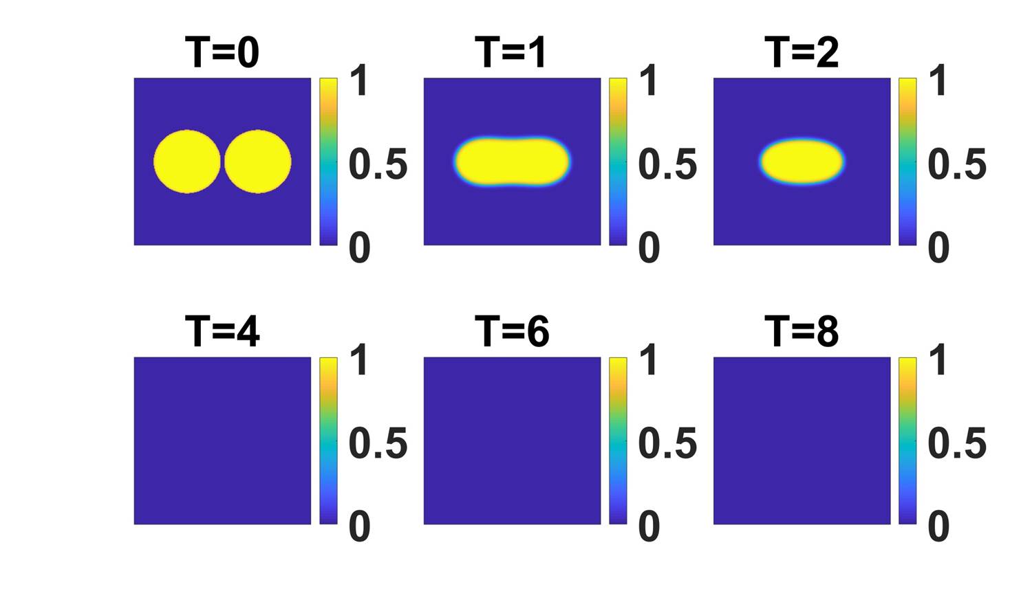
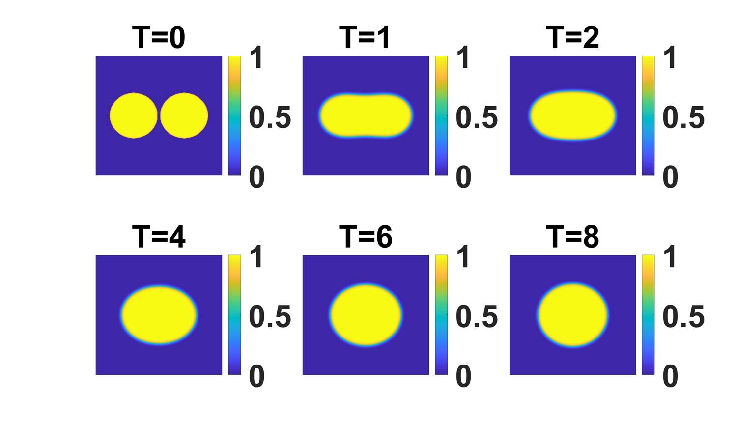
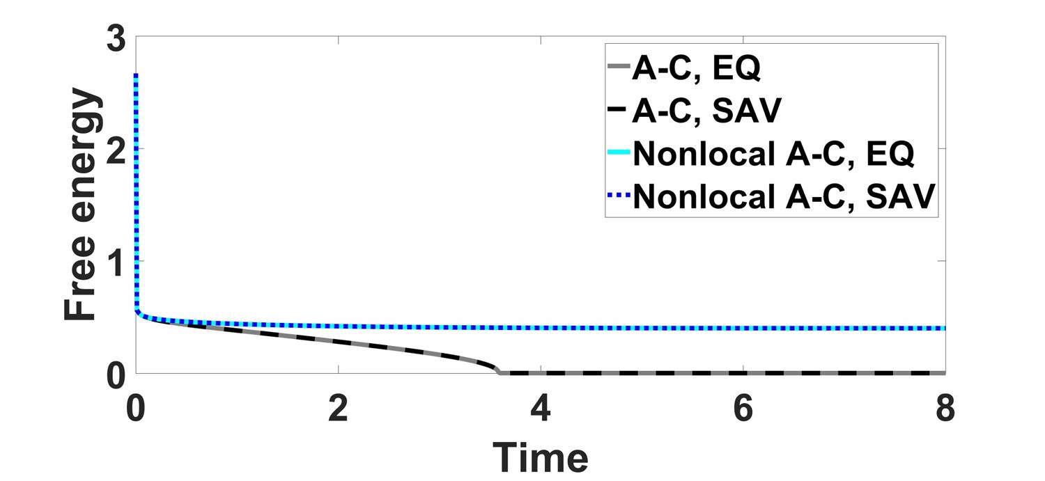
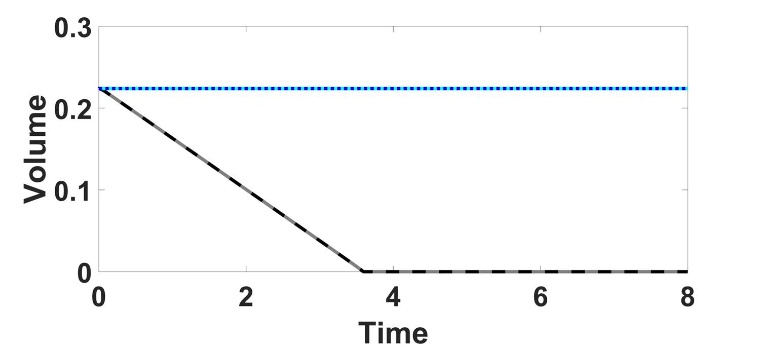
Figure 5.1: Merging of two droplets simulated using the Allen-Cahn and the Allen-Cahn models with nonlocal constraints at $M=1$. The dynamical behavior of the droplets of Allen-Cahn model and the Allen-Cahn model with nonlocal constraints is shown in (a) and (b) computed using AC-EQ and AC-L1-SAV scheme, respectively. Snapshots of the numerical approximation of volume fraction $\phi$ are taken at $\mathrm{T}=0,0.8,1.6,2.4,3.2,4$, respectively, in both cases. The time evolution of the free energy and phase volume are shown in (c) and (d), respectively. Since all other models except for the Allen-Cahn model predict the similar dynamical behavior, we only show the phase transition dynamics computed using the AC-L1-SAV scheme in (b). We compare the time evolutions of free energy and volume computed by the EQ and SAV schemes in (c) and (d). The volume computed using the Allen model vanishes before $\mathrm{T}=4$ and in the meantime the energy hits zero as well. All nonlocal Allen-Cahn models preserve the volume and dissipate energies in time. $\gamma_{1}=5\times 10^{-3}$, $\gamma_{2}=100$ are used in the computations. The temporal and spatial step are set as $\Delta t=1\times 10^{-5}$ and $h_{x}=h_{y}=1/256$, respectively.

Then, we repeat the simulations using the Allen-Cahn model with nonlocal constraints and the Cahn-Hilliard model with mobility coefficient $M=1\times 10^{-4}$. Since the coarsening rate in the Cahn-Hilliard model is much faster than that in the nonlocal Allen-Cahn models. At $\mathrm{T}=200$, the drops described by the Cahn-Hilliard model have merged into a single rounded drop, while the drops described by the nonlocal Allen-Cahn model just begin fusing. Figure 5.2-(a) and (b) depict a representative drop merging simulation using the CH-EQ scheme for the Cahn-Hilliard model and one using the AC-L1-SAV scheme for the Allen-Cahn with a nonlocal constraint, respectively. The time evolution of the free energy computed from the Cahn-Hilliard model and that from the nonlocal Allen-Cahn model is depicted in Figure 5.2-(c) and (d), respectively, in which the Cahn-Hilliard yields a smaller free energy than the nonlocal Allen-Model does. This is because at $\mathrm{T}=200$ the Cahn-Hilliard dynamics has come into the steady state comparing with the dynamics of the Allen-Cahn model with nonlocal constraints.

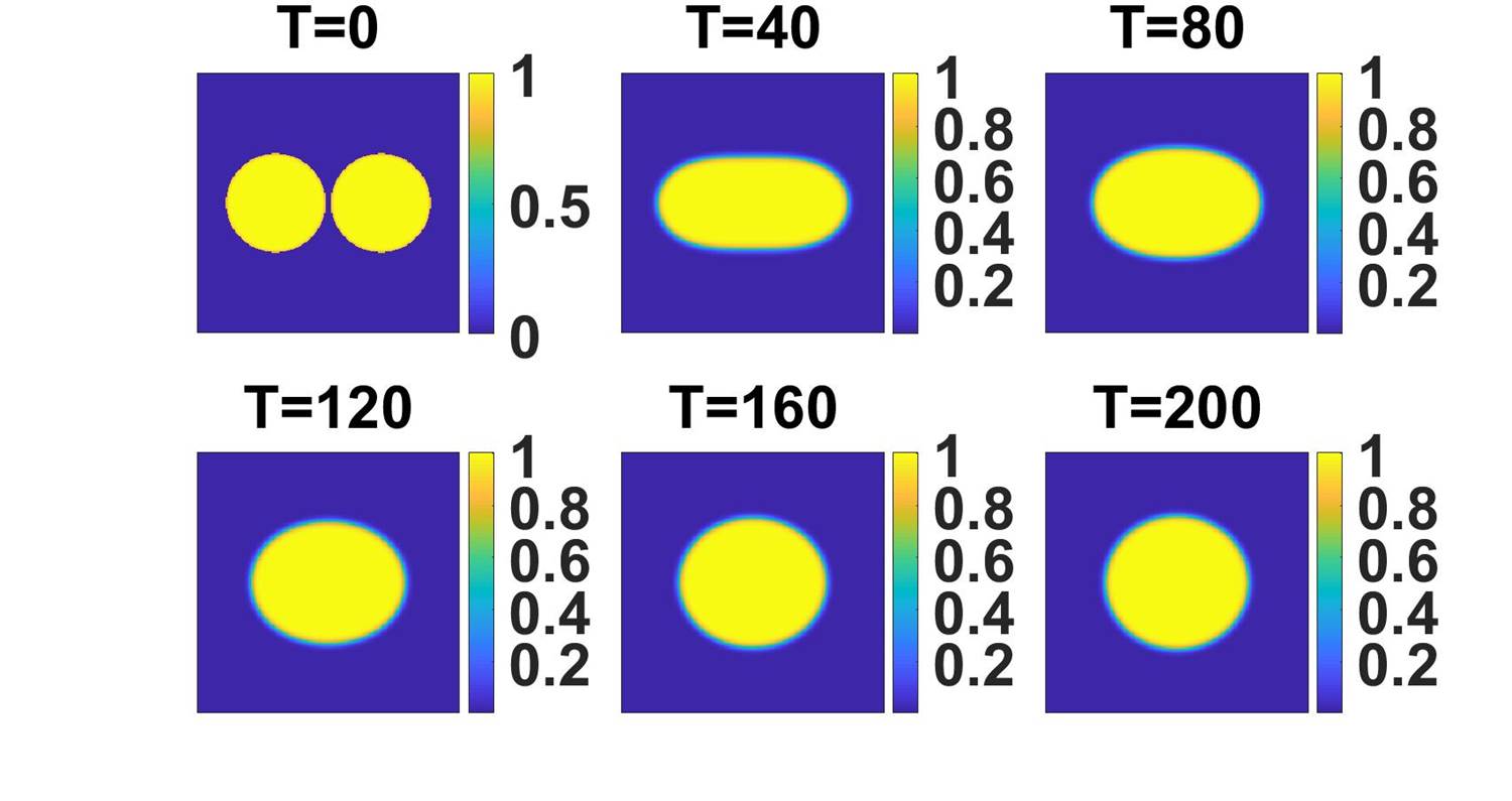
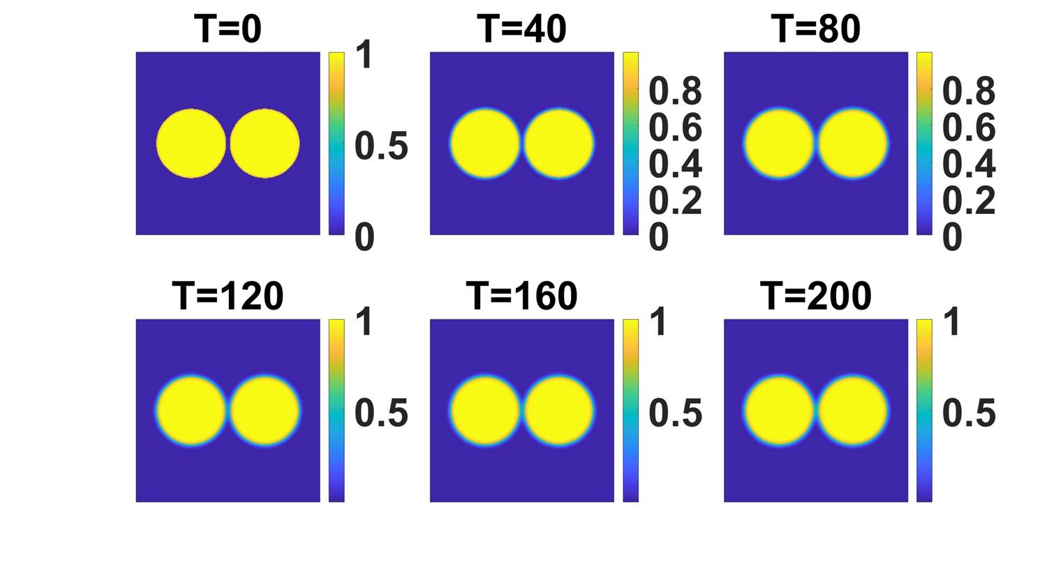
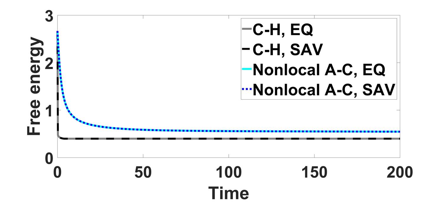
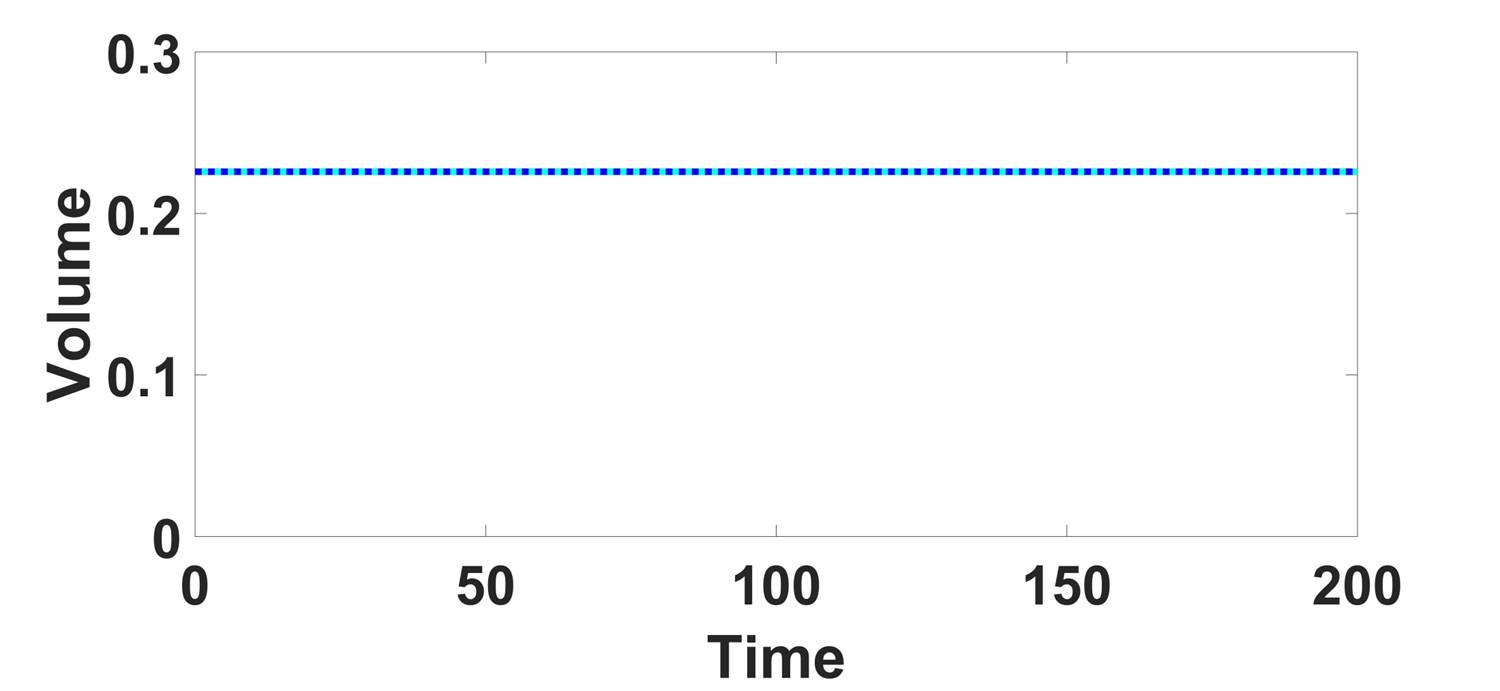
Figure 5.2: Merging of two droplets simulated using the Cahn-Hilliard and the Allen-Cahn models with nonlocal constraints at $M=1\times 10^{-4}$. The phase evolution of the droplets of Cahn-Hilliard model and the Allen-Cahn model with nonlocal constraints is shown in (a) and (b) using the CH-EQ and AC-L1-SAV scheme, respectively. Snapshots of the numerical solution of $\phi$ are taken at $\mathrm{T}=0,40,80,120,160,200$, respectively, in both cases. The time evolution of the free energy and the volume are shown in (c) and (d), respectively. The Cahn-Hilliard model and the nonlocal Allen-Cahn models preserve the same volume and dissipate energies in time. Since the energy dissipates is faster in the Cahn-Hilliard model than in the nonlocal Allen-Cahn models initially, the energy profile predicted by the former is lower than the one predicted by the latter in the simulations. We set $\gamma_{1}=5\times 10^{-3}$, $\gamma_{2}=100$ in the simulations. The temporal and spatial steps are set as $\Delta t=1\times 10^{-5}$ and $h_{x}=h_{y}=1/256$, respectively.

Secondly we use a random initial condition to assess the property of volume preserving nonlocal Allen-Cahn models in phase coarsening dynamics. Once again, The Allen-Cahn model gives one phase diagram at $t=50$, while the Allen-Cahn models with nonlocal constraints yield another at the same parameter values and initial conditions. There is simply no comparison between these two model predictions in the terminal phase diagram. Figure 5.3-(a) and (b) depict a typical simulation using the AC-EQ scheme for the Allen-Cahn model and the AC-L1-EQ scheme for the Allen-Cahn model with a Lagrangian multiplier, respectively. The time evolution of the free energy and the volume computed from the numerical schemes for the Allen-Cahn and the nonlocal Allen-Cahn models are shown in Figure 5.3- (c) and (d), respectively. Between the EQ and SAV schemes of the same model, we have yet seen any visible differences between the numerical results.

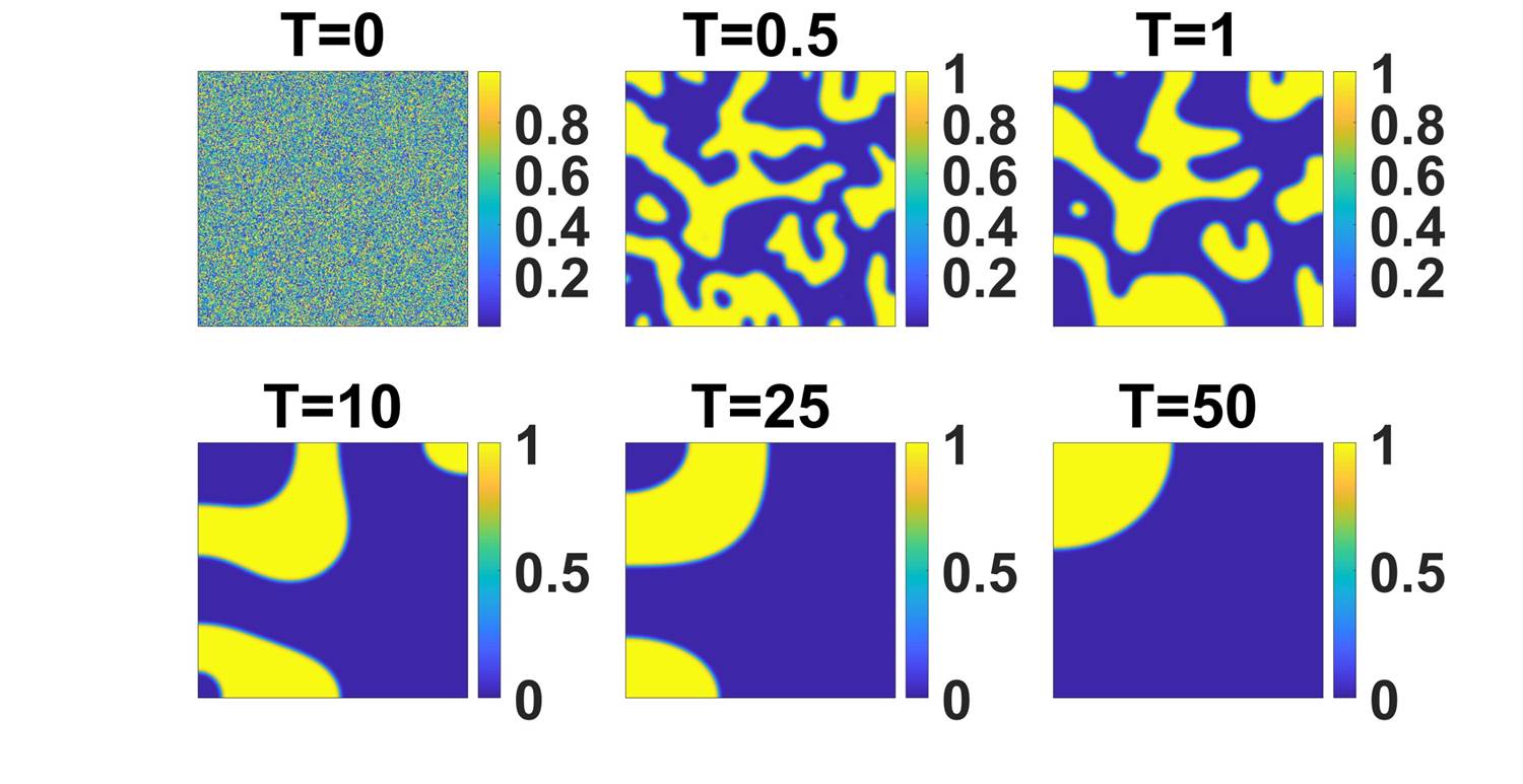
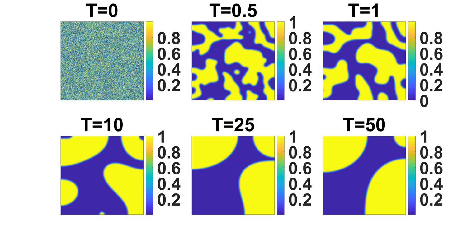
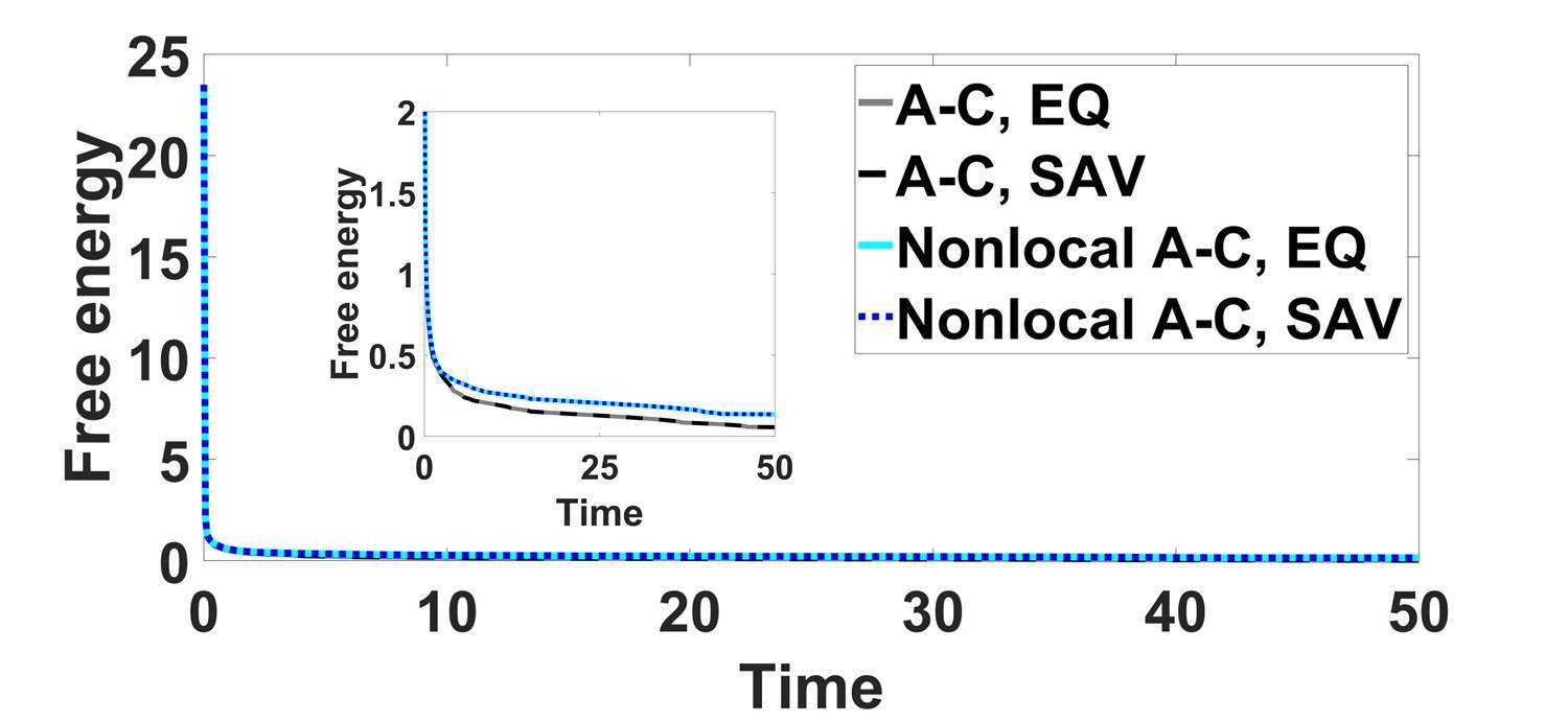
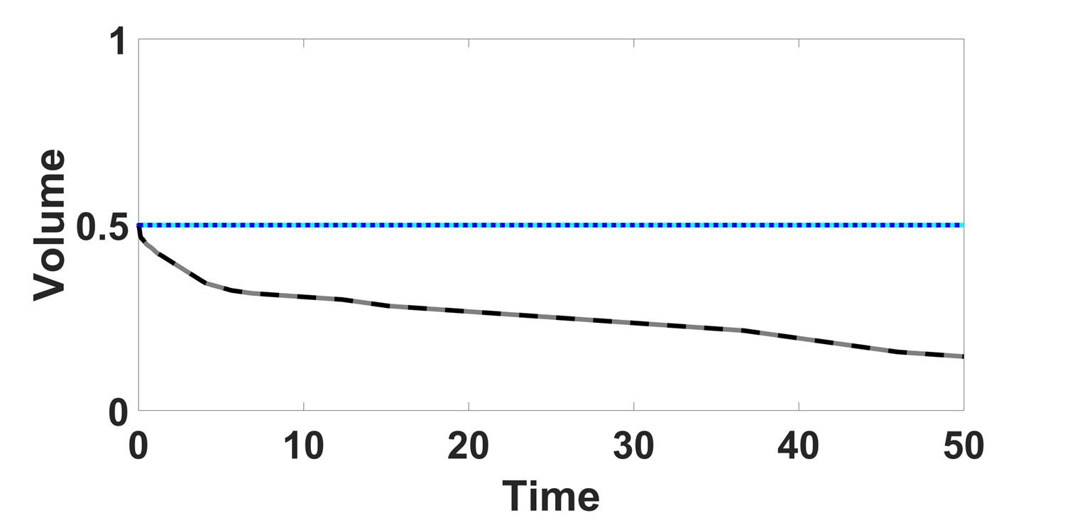
Figure 5.3: Coarsening dynamics simulated using the Allen-Cahn and the Allen-Cahn models with nonlocal constraints at $M=1$. The coarsening dynamics of Allen-Cahn model and the Allen-Cahn model with nonlocal constraints are shown in (a) and (b) using the AC-EQ and AC-L1-EQ scheme, respectively. Snapshots of the numerical approximation of $\phi$ are taken at $\mathrm{T}=0,0.5,1,10,25,50$, respectively, in both cases. The time evolution of the free energy and the volume are shown in (c) and (d), respectively. The Allen-Cahn model does not conserve the volume, while the nonlocal Allen-Cahn models preserve the volume and dissipate energies in time. The energy obtained using the Allen-Cahn model is lower than that using the nonlocal Allen-Cahn models. We set $\gamma_{1}=1\times 10^{-3}$, $\gamma_{2}=50$ in the computations. The temporal and spatial steps are set as $\Delta t=1\times 10^{-5}$ and $h_{x}=h_{y}=1/256$, respectively.

The behavior of such coarsening dynamics is also compared between the Cahn-Hilliard model and the nonlocal Allen-Cahn models. Since the coarsening rate in the Cahn-Hilliard model is faster than that in the nonlocal Allen-Cahn models, we increase the magnitude of the mobility coefficient in the Allen-Cahn model with nonlocal constraints by 1000 folds and then repeat the simulations. This speeds up the coarsening dynamics of the nonlocal Allen-Cahn system significantly, although the result from the Cahn-Hilliard model still reaches a coarser grain than that of the Allen-Cahn models with nonlocal constraints. Figure 5.4-(a) and (b) depict two representative examples on phase coarsening dynamics using CH-SAV and AC-L1-SAV schemes, respectively. Figure 5.4-(c) and (d) show the decaying free energy and the volume preserving results for the two selected simulations.

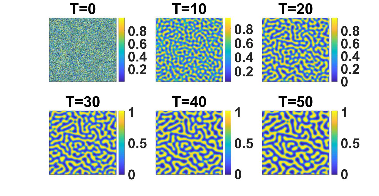
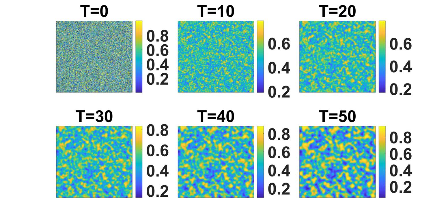
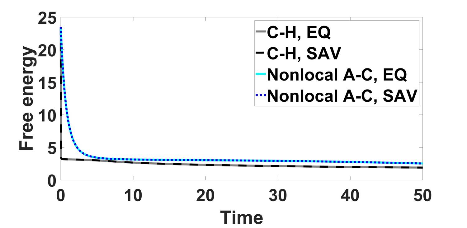
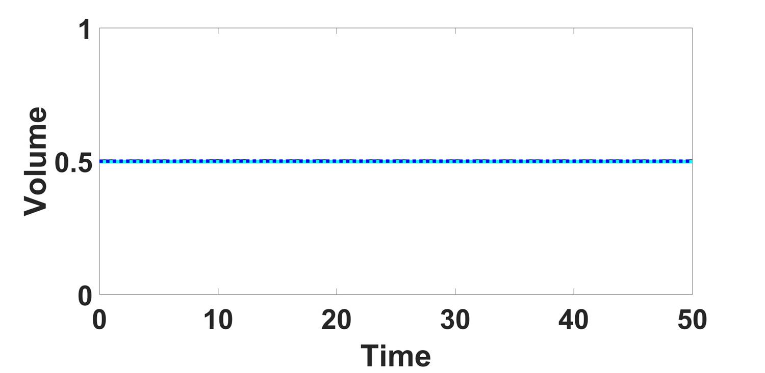
Figure 5.4: Coarsening dynamics simulated using the Cahn-Hilliard model at $M=1\times 10^{-6}$ and the Allen-Cahn models with nonlocal constraints at $M=1\times 10^{-3}$. The coarsening dynamics of the Cahn-Hilliard model and the Allen-Cahn model with nonlocal constraints are shown in (a) and (b), simulated by corresponding SAV schemes (AC-SAV and AC-L1-SAV), respectively. Snapshots of the numerical solutions of $\phi$ are taken at $\mathrm{T}=0,10,20,30,40,50$ in both cases. The time evolution of the free energy and volume are shown in (c) and (d), respectively. All models preserve the volume and dissipate energies in time. The faster coarsening dynamics in the Cahn-Hilliard model makes its energy slightly slower than the one predicted using the nonlocal Allen-Cahn models. We set $\gamma_{1}=1\times 10^{-3}$, $\gamma_{2}=50$. The temporal and spatial step sizes are set as $\Delta t=1\times 10^{-5}$ and $h_{x}=h_{y}=1/256$, respectively.

The results show the non-volume-conserving Allen-Cahn model can’t be used to simulate the merging of droplets and the coarsening dynamics accurately, whereas the Allen-Cahn model with a penalizing potential and a Lagrangian multiplier can conserve the volume as the Cahn-Hilliard model does (see Fig 5.1-5.4). Compared with the Allen-Cahn model and the Cahn-Hilliard model, the Allen-Cahn models with nonlocal constraints not only conserves the volume of the density field in domain, but also shows a slower dissipation rate than both of them. One can enlarge the mobility of the Allen-Cahn model with nonlocal constraints to accelerate the merging dynamics. We also compared the time evolution of the dissipation rates for the nonlocal Allen-Cahn models and the Cahn-Hilliard model with the same mobility coefficient $M$. The result indicates the dissipation rate of the free energy of nonlocal Allen-Cahn models is slower than that of the Cahn-Hilliard (see Fig 5.5).

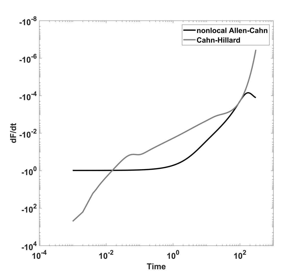
Figure 5.5: Time evolutions of the dissipation rate for the Allen-Cahn model with nonlocal constraints and the Cahn-Hilliard model (Simulated using AC-L1-SAV and CH-EQ, respectively). The dissipation rate of the energy is calculated from Fig 5.2. At $t\leq 0.02$, the dissipation rate in the Cahn-Hilliard equation is larger than that in the Allen-Cahn equations with nonlocal constraints. This explains why the Cahn-Hilliard dynamics merges drops faster than that of the Cahn-Hilliard with nonlocal constraints does.

5.2.1 Practical implementation of the schemes

Although the schemes are shown unconditionally energy stable, the numerical results are not guaranteed to be always accurate if the time step size is large due to the essentially sequential decoupling of the schemes in Fig 5.6. In all these schemes based on energy quadratization strategies, the equation for the auxiliary variables or the intermediate variables are ordinary differential equations, which are derived from original algebraic equations (which define the intermediate variables) by taking time derivatives. The numerical schemes devised to solve these ordinary differential equations may not be accurate enough to warrant the accumulation of the energy accurately.

To remedy the inherent deficiency, we propose two methods to modify the schemes in practical implementations to improve their numerical accuracy with a large time step. For simplicity, we define $f_{1}(\phi^{n})$ as the non-quadratic, nonlinear term in the bulk potential, which is $f_{1}(\phi^{n})=f(\phi^{n})-\gamma_{2}{(\phi^{n})}^{2}$ in this paper. The two methods are given below.

1. After obtaining $\phi^{n+1}$, we update $q^{n+1}$ using $q^{n+1}=\sqrt{f_{1}(\phi^{n+1})+C_{0}}$.
   

2. After obtaining $\phi^{n+1}$, if $\int_{\Omega}(q^{n+1}-\sqrt{f_{1}(\phi^{n+1})+C_{0}}\mathrm{)}d{\bf r}\leqslant\varepsilon$, we update $q^{n+1}$ using $q^{n+1}=q^{n}+\overline{q^{\prime}}^{n+1/2}(\phi^{n+1}-\phi^{n})$, otherwise, using $q^{n+1}=\sqrt{f_{1}(\phi^{n+1})+C_{0}}-\frac{2-\alpha\Delta t}{2+\alpha\Delta t}(q^{n}-\sqrt{f_{1}(\phi^{n})+C_{0}})$.

We note that, in method 2, the result is insensitive to the choice of $\alpha>0$. Figure 5.6 depicts a pair of comparative studies on drop merging simulations using the Cahn-Hilliard model and the Allen-Cahn model with a Lagrange multiplier discretized using both EQ and SAV methods. The benchmark or good results are obtained using small time steps. Using these two tricks, we can alleviate the constraints imposed on the time step size for the EQ schemes considerably. In Fig 5.7, we show results of the numerical methods at a relatively large step size. The improvement is significant. We also test our tricks for the SAV schemes, but we observe that only method 1 performs well.

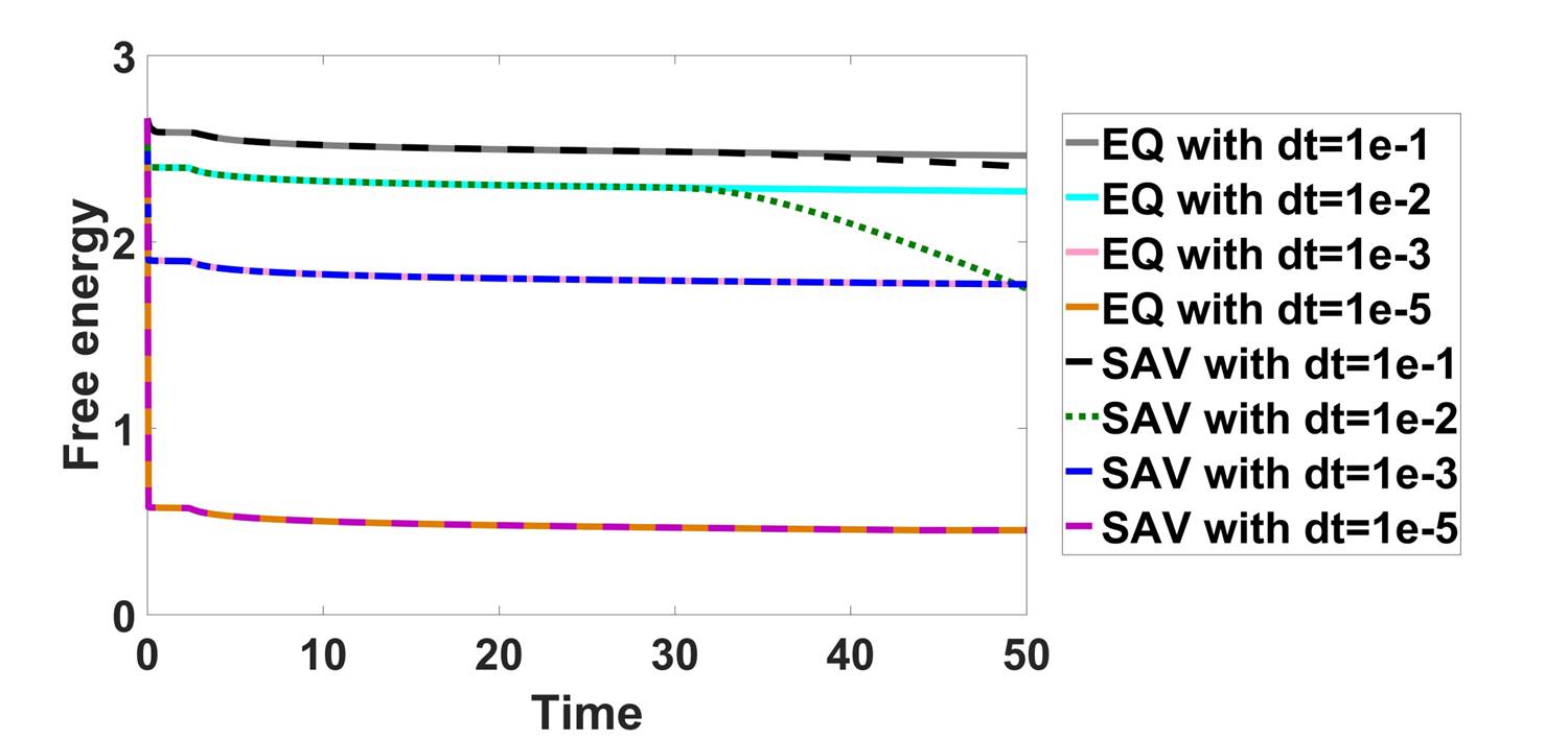
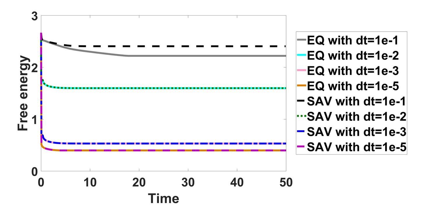
Figure 5.6: Accuracy of numerical solutions of the Cahn-Hilliard model and the Allen-Cahn model with a Lagrange multiplier. (a) The free energy computed using the Cahn-Hilliard model at four selected time steps, respectively. (b). The free energy computed using AC-L1-EQ and AC-L1-SAV schemes at four selected time steps, respectively. The time step sizes used are $1\times 10^{-1}$, $1\times 10^{-2}$, $1\times 10^{-3}$, $1\times 10^{-5}$. We use $M=1\times 10^{-4}$ for the Cahn-Hilliard model and $M=1$ for the nonlocal Allen-Cahn model. The initial condition and other model parameters are the same as those in 5.2. In the computation using the Cahn-Hilliard model, the result converges at $\Delta t=1\times 10^{-5}$. The outcome is slightly better for the Allen-Cahn model with a lagrange multiplier.

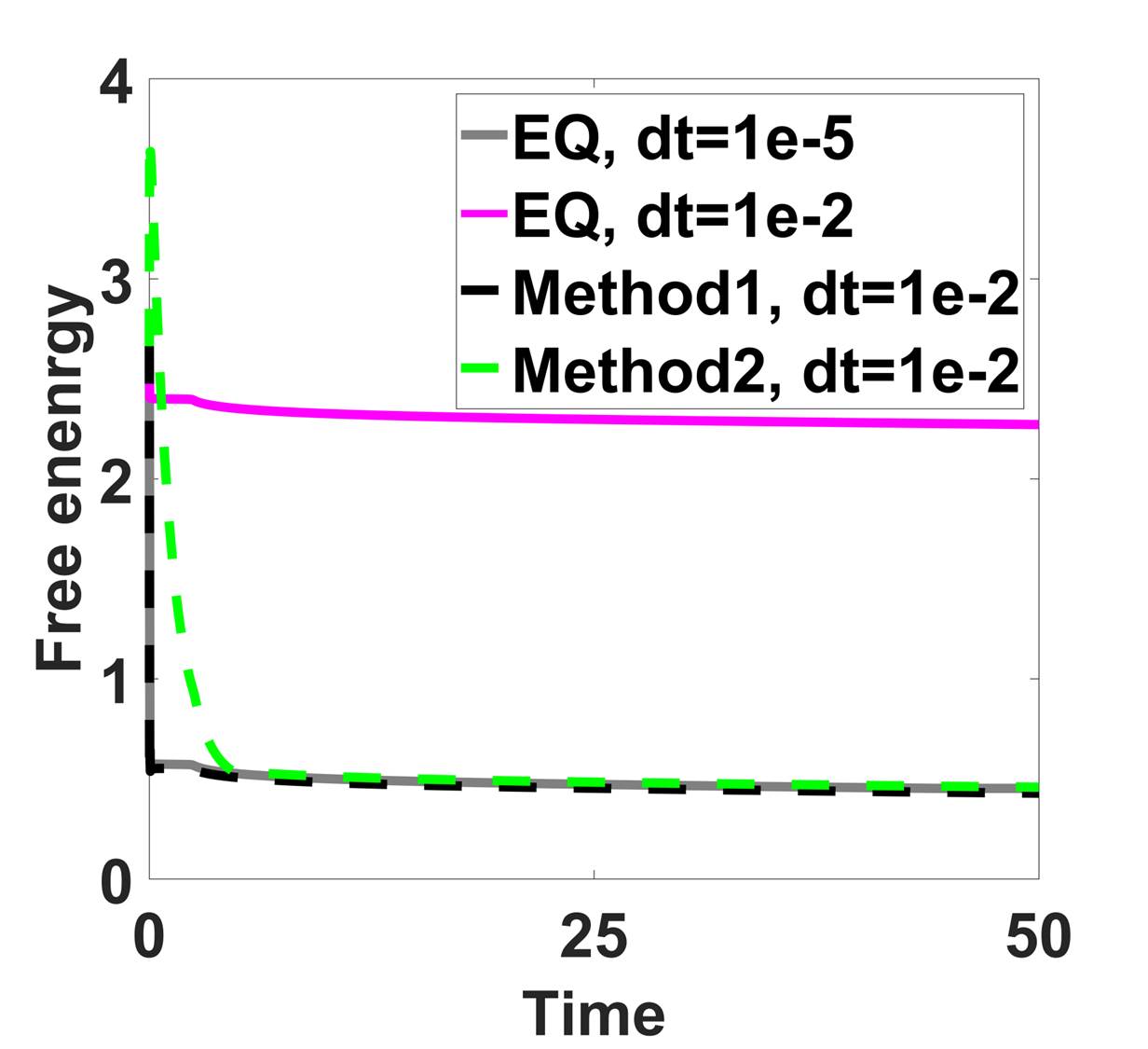
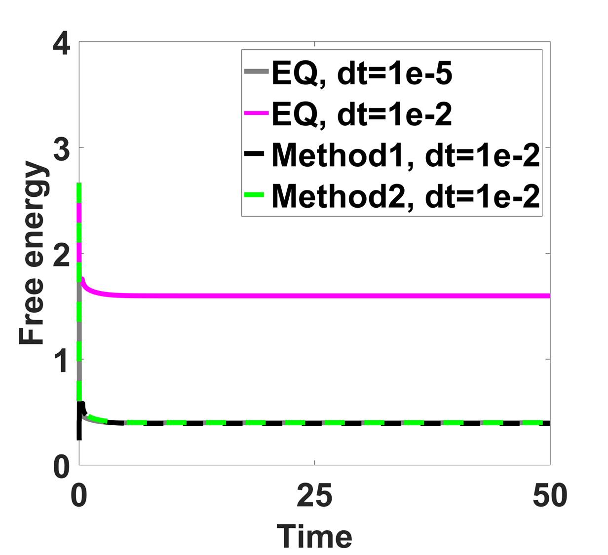
Figure 5.7: Accuracy of EQ schemes when implemented using the tricks. (a). Results computed using CH-EQ scheme. (b). Results computed using the AC-L1-EQ scheme. We use $M=1\times 10^{-4}$, $\alpha=1,C=5\times 10^{-5}$ for the Cahn-Hilliard model and $M=1$, $\alpha=1,C=1.5\times 10^{-4}$ for the Allen-Cahn model with a Lagrange multiplier in the simulations. The second numerical trick works better than the first one in the case of the nonlocal Allen-Cahn model, but the first method works better for the Cahn-Hilliard model. The initial conditions and the parameter values are the same as those used in 5.2.

In the numerical experiments, we observe that the Allen-Cahn model with a penalizing potential and the Allen-Cahn model with a Lagrange multiplier seem to render comparable numerical results. In this study, we have used two different definitions of the phase volume $V(t)=\int_{\Omega}h(\phi(t))\mathrm{d{\bf r}}$ with two choices of $h(\phi)$:

$$\begin{array}[]{l}h(\phi)=\phi,\\ h^{\prime}(\phi)=\frac{(m+1)(2m+1)}{m}[\phi(1-\phi)]^{m},m\hbox{ is a positive integer}.\end{array}$$ (5.6)

Our numerical experiments do not seem to be able to differentiate between the nonlocal Allen-Cahn models using either volume definitions. Thus both can be used at the discretion of the user in practice. Physically, the second definition seems to be more sound because the compensation to the time change of the volume fraction primarily takes place around the interface while the first definition seems to compensate the phase variable globally [24].

The phase evolution, time evolution of the volume and the free energy of the two Allen-Cahn models with nonlocal constraints simulated by EQ or SAV are essentially the same, if the penalizing parameter $\eta$ is chosen appropriately. The choice of $\eta$ can be fairly arbitrary [20]. For very large $\eta$, however, the code does not perform well in that it slows down significantly. We thus believe there exists an ”optimal” $\eta$ that renders the best result, which ought to be determined empirically in numerical implementations. We show two examples of failure at either large $\eta$ or a small $\eta$ in Fig 5.8, in which the energy is not dissipative nor the volume conserved.

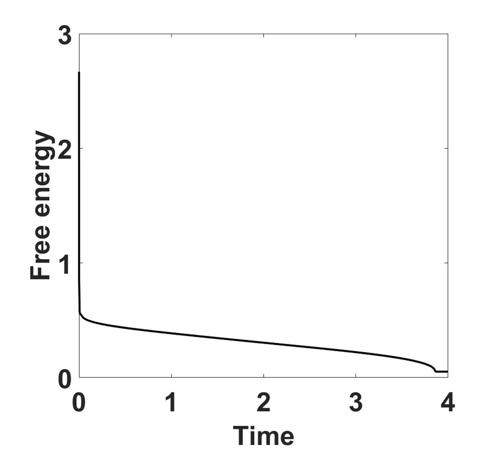
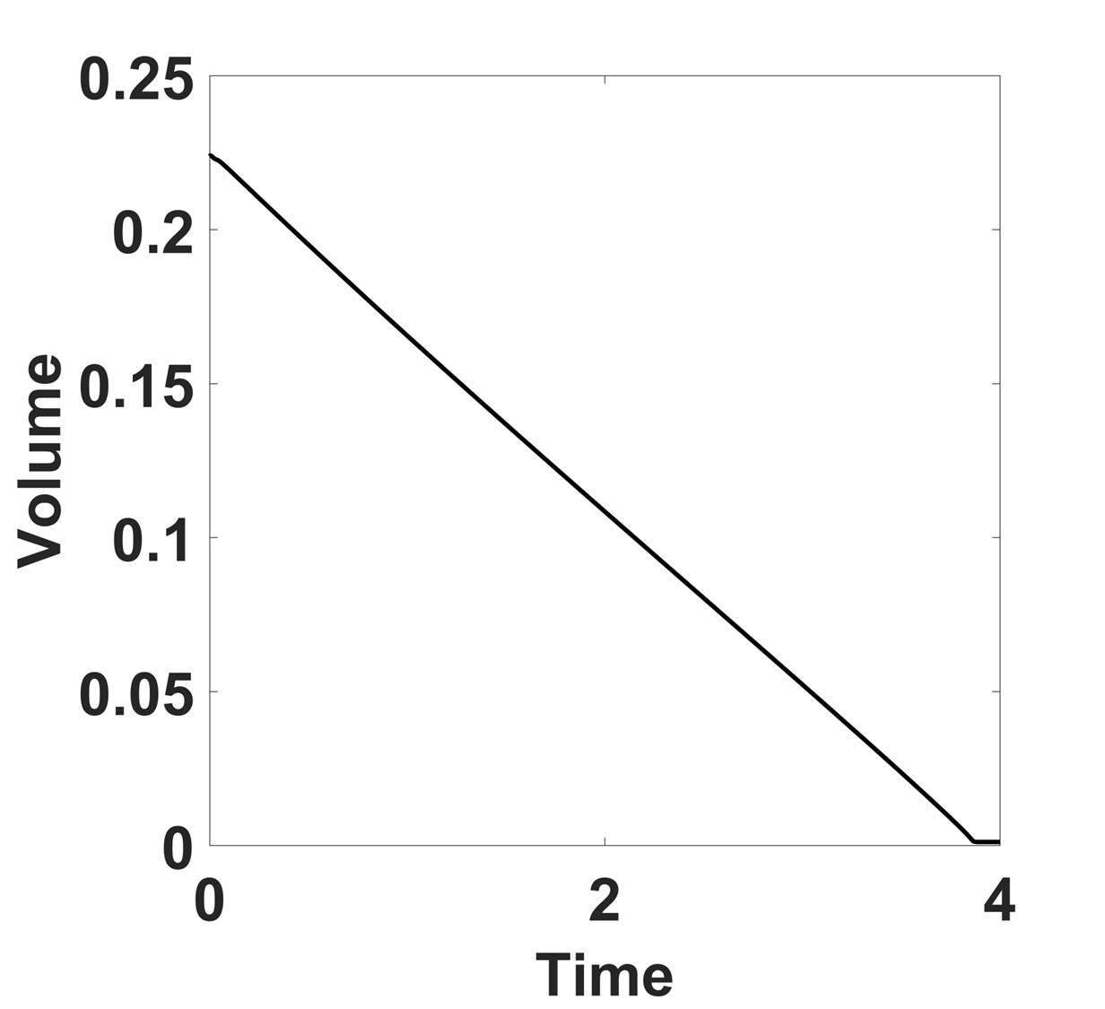
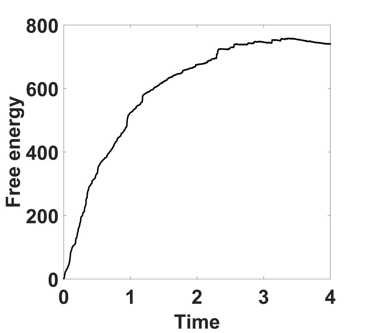
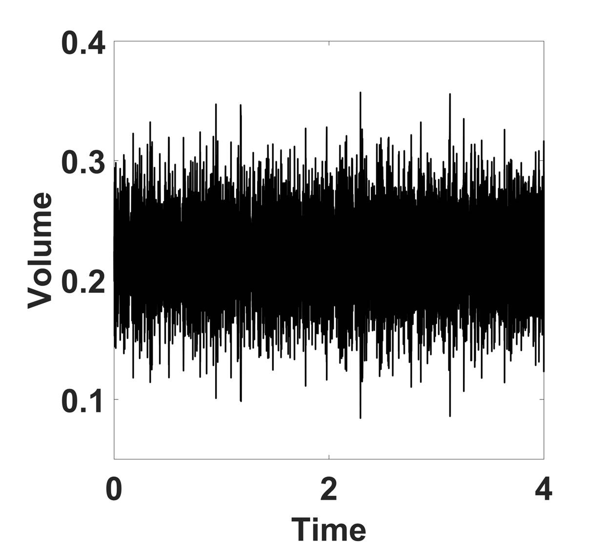
Figure 5.8: Two examples of failure for the Allen-Cahn model with a penalizing potential at $M=1$. $\eta=1$ and $\eta=1\times 10^{18}$ are chosen in the simulations. We plotted time evolution of the free energy and the volume, respectively. Results in (a) and (b) are obtained using the AC-P-EQ scheme with $\eta=1$. Results in (c) and (d) are obtained using the AC-P-SAV scheme with $\eta=1\times 10^{18}$. If $\eta$ is not ”properly chosen”, the results are not volume-conserving nor energy stable. The time step size and space time size are chosen as $\Delta t=1\times 10^{-5}$, $h_{x}=h_{y}=1/256$ in the simulations, respectively. The initial conditions and other parameters are chosen the same as those in 5.2.

In the case with a double well potential, if we define $q=\sqrt{\gamma_{2}}\phi(1-\phi)$ rather than the one in section 4.1 in the schemes, we observe a significant improvement in convergence at large time steps. This is because $q^{\prime}=\frac{\delta q}{\delta\phi}=\sqrt{\gamma_{2}}(1-2\phi)$ is a linear function, the extrapolation of $\overline{q^{\prime}}^{n+1/2}=\frac{3}{2}(q^{\prime})^{n}-\frac{1}{2}(q^{\prime})^{n-1}$ is exact. Compared with the results computed by previous schemes with large time step for nonlocal model in Fig 5.6, larger time steps can perform well in the newly developed EQ or SAV schemes in Fig 5.9. Notice that EQ schemes outperforms SAV schemes at $\Delta t=5\times 10^{-2}$ but under-performs SAV schemes at $\Delta t=1\times 10^{-2}$. Their their performance is comparable.

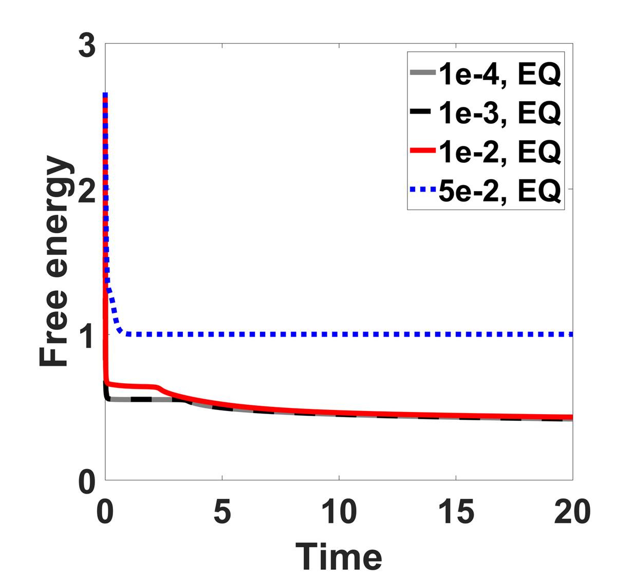
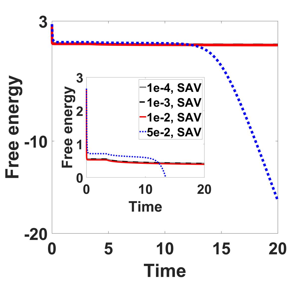
Figure 5.9: Merging of two droplets simulated by the AC-L1-EQ scheme in (a) and the AC-L1-SAV scheme in (b). The time step sizes used are $1\times 10^{-4}$, $1\times 10^{-3}$, $1\times 10^{-2}$, $5\times 10^{-2}$, respectively. The spatial mesh is $256\times 256$ in 2D. The initial conditions and other parameter values are the same as those in 5.2. At $\Delta t=0.05$, the scheme AC-L1-SAV would yield erroneous results eventually.

6 Conclusions

We have developed an exhaustive set of linear, second order, energy stable schemes for the Allen-Cahn equation with nonlocal constraints that preserve the phase volume and compared them with the energy stable, linear schemes for the Allen-Cahn and the Cahn-Hilliard models. These schemes are devised based on the energy quadratization strategy in the form of EQ and SAV format. We show that they are unconditionally energy stable and uniquely solvable. All schemes can be solved using efficient methods, making the models alternatives to the Cahn-Hilliard model to describe interface dynamics of immiscible materials while preserving the volume. The nonlocal Allen-Cahn models shows a slower coarsening rate than that of Cahn-Hilliard at the same mobility, but one can increase the mobility coefficient of the nonlocal Allen-Cahn model to accelerate their dynamics. Two implementation tricks are introduced to enhance the stability property as well as the accuracy of the numerical schemes at a large step size, but the second method doesn’t work well on the SAV schemes. In addition, we have compared the two Allen-Cahn models with nonlocal constraints numerically. The computational efficiency of the Allen-Cahn model with a penalizing potential is slightly than the one with a Lagrange multiplier, but the accuracy of the former depends on a suitable choice of model parameter $\eta$. Through numerical experiments, we show that the practical implementation using the defining algebraic functions for the auxiliary variable makes the EQ scheme superior to the SAV scheme in their computational efficiency and accuracy. When the equation of the auxiliary variable can be solved more accurately, large time step size can be applied. In the end, we note that the size of mobility and the time step size are dominating factors that determine ultimately the efficiency and accuracy of the schemes.

Appendix

Appendix A Sherman-Morrison formula and its application to solving the integro-differential equation

Here we give a brief review on the Sherman-Morrison formula [2] and explain its applications in the practical implementation of our various relevant schemes.

Suppose $A$ is an invertible square matrix, and $u$,$v$ are column vectors. Then $A+uv^{T}$ is invertible iff $1+v^{T}A^{-1}u\neq 0$. If $A+uv^{T}$ is invertible, then its inverse is given by

$$\begin{array}[]{l}(A+uv^{T})^{-1}=A^{-1}-\frac{A^{-1}uv^{T}A^{-1}}{1+v^{T}A^{-1}u}.\end{array}$$ (A.2)

So if $Ay=b$ and $Az=u$, $(A+uv^{T})x=b$ has the solution given by

$$\begin{array}[]{l}x=y-\frac{v^{T}y}{1+v^{T}z}z.\end{array}$$ (A.4)

For the integral term(s) in the semi-discrete schemes in this study such as (4.78), we need to discretize it properly. $\forall f$, we discretize $\int_{\Omega}f\mathrm{d{\bf r}}$ using the composite trapezoidal rule and adding all the elements of the new matrix $w_{1}w_{2}^{T}f$, where $w_{1}=\frac{h_{x}}{2}S$, $w_{2}=\frac{h_{y}}{2}S$, $h_{x}$, $h_{y}$ are the spatial step sizes and $S={[1,2,2,...,2,2,1]}^{T}$. For convenience, we use $w_{1}w_{2}^{T}f$ to represent the integral discretized by the composite trapezoidal rule.

To solve equation (4.78), we discretize the integral or the inner product of functions $(c,\phi^{n+1})d$ as $u{v}^{T}\phi^{n+1}$. The scheme is recast to $A\phi^{n+1}+u{v}^{T}\phi^{n+1}=b^{n}$. After using the Sherman-Morrison formula, we get

$$\begin{array}[]{l}\phi^{n+1}=A^{-1}{b}^{n}-\frac{{v}^{T}{A}^{-1}{{b}}^{n}}{{1+{v}^{T}A}^{-1}u}{A}^{-1}u,\end{array}$$ (A.6)

In the inner product of vectors, (4.78) can be rewritten into

$$\begin{array}[]{l}{\phi}^{n+1}=A^{-1}{b}^{n}-\frac{\langle c,A^{-1}b^{n}\rangle}{1+\langle c,A^{-1}d\rangle}{A}^{-1}d.\end{array}$$ (A.8)

So, indeed the approach we take in the study using discrete inner product is essentially equivalent to applying the Sherman-Morrison formula.

References

• [1] Samuel M Allen and John W Cahn. A microscopic theory for antiphase boundary motion and its application to antiphase domain coarsening. Acta Metallurgica, 27(6):1085–1095, 1979.
• [2] E Bodewig. Matrix calculus, north, p17, 1959.
• [3] Samira Boussaıd, Danielle Hilhorst, and Thanh Nam Nguyen. Convergence to steady state for the solutions of a nonlocal reaction-diffusion equation. Evolution Equations and Control Theory, 2015.
• [4] John W Cahn and John E Hilliard. Free energy of a nonuniform system. i. interfacial free energy. The Journal of chemical physics, 28(2):258–267, 1958.
• [5] Lizhen Chen, Jia Zhao, and Xiaofeng Yang. Regularized linear schemes for the molecular beam epitaxy model with slope selection. Applied Numerical Mathematics, 128:139–156, 2018.
• [6] Wenbin Chen, Daozhi Han, and Xiaoming Wang. Uniquely solvable and energy stable decoupled numerical schemes for the cahn–hilliard–stokes–darcy system for two-phase flows in karstic geometry. Numerische Mathematik, 137(1):229–255, 2017.
• [7] Yuanzhen Cheng, Alexander Kurganov, Zhuolin Qu, and Tao Tang. Fast and stable explicit operator splitting methods for phase-field models. Journal of Computational Physics, 303:45–65, 2015.
• [8] Masao Doi and Samuel Frederick Edwards. The theory of polymer dynamics, volume 73. oxford university press, 1988.
• [9] Suchuan Dong, Zhiguo Yang, and Lianlei Lin. A family of second-order energy-stable schemes for cahn-hilliard type equations. arXiv preprint arXiv:1803.06047, 2018.
• [10] Qiang Du, Lili Ju, Xiao Li, and Zhonghua Qiao. Stabilized linear semi-implicit schemes for the nonlocal cahn–hilliard equation. Journal of Computational Physics, 363:39–54, 2018.
• [11] Charles M Elliott and AM Stuart. The global dynamics of discrete semilinear parabolic equations. SIAM journal on numerical analysis, 30(6):1622–1663, 1993.
• [12] David J Eyre. Unconditionally gradient stable time marching the cahn-hilliard equation. MRS Online Proceedings Library Archive, 529, 1998.
• [13] Xiaolin Fan, Jisheng Kou, Zhonghua Qiao, and Shuyu Sun. A componentwise convex splitting scheme for diffuse interface models with van der waals and peng–robinson equations of state. SIAM Journal on Scientific Computing, 39(1):B1–B28, 2017.
• [14] Yuezheng Gong, Jia Zhao, and Qi Wang. Linear second order in time energy stable schemes for hydrodynamic models of binary mixtures based on a spatially pseudospectral approximation. Advances in Computational Mathematics, pages 1–28, 2018.
• [15] Yuezheng Gong, Jia Zhao, Xiaogang Yang, and Qi Wang. Fully discrete second-order linear schemes for hydrodynamic phase field models of binary viscous fluid flows with variable densities. Siam Journal on Scientific Computing, 40(1):B138–B167, 2018.
• [16] Ruihan Guo and Yan Xu. Local discontinuous galerkin method and high order semi-implicit scheme for the phase field crystal equation. SIAM Journal on Scientific Computing, 38(1):A105–A127, 2016.
• [17] Morton E Gurtin, Debra Polignone, and Jorge Vinals. Two-phase binary fluids and immiscible fluids described by an order parameter. Mathematical Models and Methods in Applied Sciences, 6(06):815–831, 1996.
• [18] Daozhi Han and Xiaoming Wang. A second order in time, uniquely solvable, unconditionally stable numerical scheme for cahn–hilliard–navier–stokes equation. Journal of Computational Physics, 290:139–156, 2015.
• [19] F. M. Leslie. Theory of flow phenomena in liquid crystals. Advances in Liquid Crystals, 4:1–81, 1979.
• [20] Hongwei Li, Lili Ju, Chenfei Zhang, and Qiujin Peng. Unconditionally energy stable linear schemes for the diffuse interface model with peng–robinson equation of state. Journal of Scientific Computing, 75(2):993–1015, 2018.
• [21] Lars Onsager. Reciprocal relations in irreversible processes. i. Physical review, 37(4):405, 1931.
• [22] Lars Onsager. Reciprocal relations in irreversible processes. ii. Physical review, 38(12):2265, 1931.
• [23] R. A. Pethrick. The theory of polymer dynamics m. doi and s. f. edwards, oxford university press. Journal of Chemical Technology and Biotechnology Biotechnology, 44(1):79–80, 1988.
• [24] Jacob Rubinstein and Peter Sternberg. Nonlocal reaction diffusion equations and nucleation. Ima Journal of Applied Mathematics, 48(3):249–264, 1992.
• [25] Jie Shen, Cheng Wang, Xiaoming Wang, and Steven M Wise. Second-order convex splitting schemes for gradient flows with ehrlich–schwoebel type energy: application to thin film epitaxy. SIAM Journal on Numerical Analysis, 50(1):105–125, 2012.
• [26] Jie Shen, Jie Xu, and Jiang Yang. The scalar auxiliary variable (sav) approach for gradient flows. Journal of Computational Physics, 353:407–416, 2018.
• [27] Jie Shen and Xiaofeng Yang. Numerical approximations of allen-cahn and cahn-hilliard equations. Discrete Contin. Dyn. Syst, 28(4):1669–1691, 2010.
• [28] Cheng Wang, Xiaoming Wang, and Steven M Wise. Unconditionally stable schemes for equations of thin film epitaxy. Discrete Contin. Dyn. Syst, 28(1):405–423, 2010.
• [29] Lin Wang and Haijun Yu. On efficient second order stabilized semi-implicit schemes for the cahn–hilliard phase-field equation. Journal of Scientific Computing, pages 1–25, 2017.
• [30] Steven M Wise, Cheng Wang, and John S Lowengrub. An energy-stable and convergent finite-difference scheme for the phase field crystal equation. SIAM Journal on Numerical Analysis, 47(3):2269–2288, 2009.
• [31] Xiaofeng Yang. Efficient schemes with unconditionally energy stability for the anisotropic cahn-hilliard equation using the stabilized-scalar augmented variable (s-sav) approach. arXiv preprint arXiv:1804.02619, 2018.
• [32] Xiaofeng Yang and Lili Ju. Linear and unconditionally energy stable schemes for the binary fluid csurfactant phase field model. Computer Methods in Applied Mechanics and Engineering, 318:1005–1029, 2017.
• [33] Xiaofeng Yang, Jia Zhao, and Qi Wang. Numerical approximations for the molecular beam epitaxial growth model based on the invariant energy quadratization method. Journal of Computational Physics, 333:104–127, 2017.
• [34] Xiaogang Yang, Yuezheng Gong, Jun Li, Jia Zhao, and Qi Wang. On hydrodynamic phase field models for binary fluid mixtures. Theoretical and Computational Fluid Dynamics, pages 1–24, 2017.
• [35] Jia Zhao, Yuezheng Gong, and Qi Wang. Aritrary high order unconditionally energy stable schemes for gradient flow models. Journal of Computational Physics, 2018.
• [36] Jia Zhao, Qi Wang, and Xiaofeng Yang. Numerical approximations to a new phase field model for two phase flows of complex fluids. Computer Methods in Applied Mechanics and Engineering, 310:77–97, 2016.
• [37] Jia Zhao, Qi Wang, and Xiaofeng Yang. Numerical approximations for a phase field dendritic crystal growth model based on the invariant energy quadratization approach. International Journal for Numerical Methods in Engineering, 110(3), 2017.
• [38] Jia Zhao, Xiaofeng Yang, Yuezheng Gong, and Qi Wang. A novel linear second order unconditionally energy stable scheme for a hydrodynamic-tensor model of liquid crystals. Computer Methods in Applied Mechanics and Engineering, 318:803–825, 2017.
• [39] Jia Zhao, Xiaofeng Yang, Yuezheng Gong, Xueping Zhao, Xiaogang Yang, Jun Li, and Qi Wang. A general strategy for numerical approximations of non-equilibrium models–part i: Thermodynamical systems. International Journal of Numerical Analysis & Modeling, 15(6):884–918, 2018.
• [40] Jia Zhao, Xiaofeng Yang, Jun Li, and Qi Wang. Energy stable numerical schemes for a hydrodynamic model of nematic liquid crystals. SIAM Journal on Scientific Computing, 38(5):A3264–A3290, 2016.
• [41] Jia Zhao, Xiaofeng Yang, Jie Shen, and Qi Wang. A decoupled energy stable scheme for a hydrodynamic phase-field model of mixtures of nematic liquid crystals and viscous fluids. Journal of Computational Physics, 305:539–556, 2016.