A single-world consistent interpretation of quantum mechanics from fundamental time and length uncertainties

Abstract

Within ordinary —unitary— quantum mechanics there exist global protocols that allow to verify that no definite event —an outcome to which a probability can be associated— occurs. Instead, states that start in a coherent superposition over possible outcomes always remain as a superposition. We show that, when taking into account fundamental errors in measuring length and time intervals, that have been put forward as a consequence of a conjunction of quantum mechanical and general relativity arguments, there are instances in which such global protocols no longer allow to distinguish whether the state is in a superposition or not. All predictions become identical as if one of the outcomes occurs, with probability determined by the state. We use this as a criteria to define events, as put forward in the Montevideo Interpretation of Quantum Mechanics. We analyze in detail the occurrence of events in the paradigmatic case of a particle in a superposition of two different locations. We argue that our approach provides a consistent (C) single-world (S) picture of the universe, thus allowing an economical way out of the limitations imposed by a recent theorem by Frauchiger and Renner showing that having a self-consistent single-world description of the universe is incompatible with quantum theory. In fact, the main observation of this paper may be stated as follows: If quantum mechanics is extended to include gravitational effects to a QG theory, then QG, S, and C are satisfied.

A crucial feature of quantum mechanics is that, in general, the state of a quantum system cannot be interpreted as a classical probability distribution. In particular, when a closed system $\mathcal{S}$ is found in a coherent superposition of a set of orthonormal states $\{\left|\varphi_{j}\right\rangle\!\vphantom{\left(\varphi_{j}\right)^{A}}\}$,

$$\rho_{\mathcal{S}}=\sum_{jk}\alpha_{j}\alpha^{*}_{k}\left|\varphi_{j}\right\rangle\!\vphantom{\left(\varphi_{j}\right)^{A}}\!\left\langle\varphi_{k}\right|\vphantom{\left(\varphi_{k}\right)^{A}},$$ (1)

with $\sum_{j}|\alpha_{j}|^{2}=1$, one cannot view $\mathcal{S}$ as being described by a classical probability distribution over the states $\{\left|\varphi_{j}\right\rangle\!\vphantom{\left(\varphi_{j}\right)^{A}}\}$. This is in stark contrast to the case of a system in a state

$$\rho_{\mathcal{S}}^{\text{event}}=\sum_{j}|\alpha_{j}|^{2}\left|\varphi_{j}\right\rangle\!\vphantom{\left(\varphi_{j}\right)^{A}}\!\left\langle\varphi_{j}\right|\vphantom{\left(\varphi_{j}\right)^{A}}.$$ (2)

For the latter, all subsequent dynamics and predictions are exactly as if the system had been described by a classical probability distribution over the states $\{\left|\varphi_{j}\right\rangle\!\vphantom{\left(\varphi_{j}\right)^{A}}\}$. Note that we demand $\mathcal{S}$ to be a closed system. In fact, condition (2) is not sufficient for open systems, for instance for systems that are entangled with other systems, in which case state (2) only represents a reduced density matrix.

The measurement postulate in quantum mechanics presumes that, on performing a projective measurement on the basis $\{\left|\varphi_{j}\right\rangle\!\vphantom{\left(\varphi_{j}\right)^{A}}\}$, a definite transition from $\rho_{\mathcal{S}}$ to $\rho_{\mathcal{S}}^{\text{event}}$ occurs. Thereafter, when a particular outcome is observed, the state of the system is updated to reflect the observed outcome, much the same way as is done when one replaces one’s knowledge after observing ‘heads’ on a coin toss. This change from $\rho_{\mathcal{S}}$ to $\rho_{\mathcal{S}}^{\text{event}}$ through a measurement is in stark contrast to what occurs in classical physics, where the role of a measurement is merely that of information acquisition. It is also in stark contrast with a unitary evolution of the system $\mathcal{S}$. Hence, our stance is that a complete understanding of quantum theory rests on adequately characterizing what does and does not constitute a measurement.

In this paper we solve the above conundrum by providing a definite criterion for the physical means by which a transition from an arbitrary quantum state $\rho_{\mathcal{S}}$ of a closed system to a classically interpretable state $\rho_{\mathcal{S}}^{\text{event}}$ occurs. We call such transition an event.

Note that, within realist interpretations of quantum theory, the problem of explaining the transition no event $\rightarrow$ event does not pertain to a particular view about the ontological status assigned to the wavefunction. As long as one believes that situations exist in which physical predictions for the system change when going from $\rho_{\mathcal{S}}$ to $\rho_{\mathcal{S}}^{\text{event}}$, then a criterion is needed to explain how, and under which conditions, this change occurs. Such a physical change occurs even in models in which the state is assumed to have an epistemological nature Spekkens (2007); Leifer (2014). Indeed, in this article we do not need to take any stance on the status of the wavefunction, it suffices to say that it is the best tool available to predict future dynamics. Moreover, while our derivations are in the Schrödinger picture, the state is not a fundamental entity, and the arguments could be done purely in terms of observables in the Heisenberg picture instead.

In previous works we showed how fundamental uncertainties in the measurement of time and spin components, stemming from quantum mechanical and general relativistic arguments, can be used to surmount such problem in a particular model of a spin interacting with a spin bath environment Gambini et al. (2010), and provided a criterion for the production of events Gambini et al. (2011a). This set the foundations for a realist interpretation of quantum theory: the Montevideo Interpretation Gambini and Pullin (2009); Gambini et al. (2011b); Gambini and Pullin (2018). The main point of this paper, however, does not depend on the Montevideo Interpretation but just reinforces one of its basic observations.

Here we extend the solution to a general class of global protocols that apply to any decoherence model. In this way, we provide a criterion that works in much more general settings. Our analysis also permits to provide estimates for bounds on the time of event occurrence in the paradigmatic situation of a delocalized particle in a coherent superposition over two different locations.

The structure of the paper is as follows. Section I reviews the process of environmental decoherence, and its relevance to measurement processes. In Section II we introduce global protocols that, within unitary quantum mechanics, allow to verify that no definite event can occur. Section III is devoted to fundamental time and length uncertainties, that have been argued in the past to be a consequence of combining general arguments from quantum theory and from general relativity. The core of the article can be found in Sections IV and V, where we show the physical process that leads to production of events, and that such production is definite rather than for all practical purposes, respectively. In Section VI we explain how this results in a consistent single-world description of the universe. We end in VII with a discussion.

I Evolution of non-isolated systems

It can be argued that a breakthrough on the understanding of measurements in quantum mechanics has been made in the past decades from acknowledging that measurements are performed by devices that interact with an environment Zeh (1970). In this section we review what typically happens in cases of a system interacting with an environment.

Consider that $\mathcal{S}$ interacts with an environment $\mathcal{E}$. For simplicity we assume that both are initially in a pure state, $\rho_{\mathcal{S}}(0)$ (given by Eq. (2)) and $\left|E_{r}\right\rangle\!\vphantom{\left(E_{r}\right)^{A}}\!\left\langle E_{r}\right|\vphantom{\left(E_{r}\right)^{A}}$ respectively, and that they are uncorrelated. That is, the joint initial state is

$$\rho_{\mathcal{S}\mathcal{E}}(0)=\rho_{\mathcal{S}}(0)\otimes\left|E_{r}\right\rangle\!\vphantom{\left(E_{r}\right)^{A}}\!\left\langle E_{r}\right|\vphantom{\left(E_{r}\right)^{A}}.$$ (3)

Following the standard setup for the interaction of a measuring device with an environment, let us assume the total Hamiltonian can be decomposed into a system part $H_{\mathcal{S}}$, an environmental part $H_{\mathcal{E}}$, and an interaction term $H_{I}$ (this presumes an identification of some system of interest):

$$H=H_{\mathcal{S}}\otimes\mathbbm{1}_{\mathcal{E}}+\mathbbm{1}_{\mathcal{S}}\otimes H_{\mathcal{E}}+H_{I},$$ (4)

and that

$$\left[\left|\varphi_{j}\right\rangle\!\vphantom{\left(\varphi_{j}\right)^{A}}\!\left\langle\varphi_{j}\right|\vphantom{\left(\varphi_{j}\right)^{A}}\otimes\mathbbm{1}_{\mathcal{E}},H\right]=0\quad\forall j.$$ (5)

In such a case $\{\left|\varphi_{j}\right\rangle\!\vphantom{\left(\varphi_{j}\right)^{A}}\}$ is stable under the interaction with the environment, and is referred to as a pointer basis. For simplicity we focus on exact commutation with the full Hamiltonian, but the conclusions that follow also hold for $\left[\left|\varphi_{j}\right\rangle\!\vphantom{\left(\varphi_{j}\right)^{A}}\!\left\langle\varphi_{j}\right|\vphantom{\left(\varphi_{j}\right)^{A}}\otimes\mathbbm{1}_{\mathcal{E}},H_{I}\right]=0$ in the strong measurement limit, in which $H_{I}$ dominates the evolution Paz and Zurek (1999).

According to quantum theory the closed combined $\mathcal{S}+\mathcal{E}$ system evolves unitarily, with a state at time $t$ given by

$$\rho_{\mathcal{S}\mathcal{E}}(t) =e^{-iHt/\hbar}\rho_{\mathcal{S}\mathcal{E}}(0)e^{iHt/\hbar}$$

$$=\sum_{jk}\alpha_{j}\alpha^{*}_{k}\left|\varphi_{j}\right\rangle\!\vphantom{\left(\varphi_{j}\right)^{A}}\!\left\langle\varphi_{k}\right|\vphantom{\left(\varphi_{k}\right)^{A}}\otimes\left|E_{j}(t)\right\rangle\!\vphantom{\left(E_{j}(t)\right)^{A}}\!\left\langle E_{k}(t)\right|\vphantom{\left(E_{k}(t)\right)^{A}},$$ (6)

with the environmental states evolving according to

$$\left|E_{j}(t)\right\rangle\!\vphantom{\left(E_{j}(t)\right)^{A}}=e^{-iH_{j}t/\hbar}\left|E_{r}\right\rangle\!\vphantom{\left(E_{r}\right)^{A}},$$ (7)

where $H_{j}\equiv\left\langle\varphi_{j}\right|\vphantom{\left(\varphi_{j}\right)^{A}}H\left|\varphi_{j}\right\rangle\!\vphantom{\left(\varphi_{j}\right)^{A}}$ is the effective Hamiltonian that acts on the environment given that the system is in state $\left|\varphi_{j}\right\rangle\!\vphantom{\left(\varphi_{j}\right)^{A}}$.

If the environment is large, correlations generated between system and environment typically cause rapid decay of the term $\left\langle E_{j}(t)\right|\vphantom{\left(E_{j}(t)\right)^{A}}E_{k}(t)\rangle$ Schlosshauer (2005). For many decoherence models this decay is exponential (see Schlosshauer (2014) and references within):

$$\left\langle E_{j}(t)\right|\vphantom{\left(E_{j}(t)\right)^{A}}E_{k}(t)\rangle\approx\left\langle E_{j}(0)\right|\vphantom{\left(E_{j}(0)\right)^{A}}E_{k}(0)\rangle e^{-t/\tau_{D}},\qquad j\neq k$$ (8)

where the decoherence timescale $\tau_{D}$ grows with the size of the bath. In this way, the state of the system, $\rho_{\mathcal{S}}(t)~{}=~{}\text{Tr}_{\mathcal{E}}\left[\rho(t)\right]$, given by

$$\rho_{\mathcal{S}}(t) =\sum_{jk}\alpha_{j}\alpha^{*}_{k}\left|\varphi_{j}\right\rangle\!\vphantom{\left(\varphi_{j}\right)^{A}}\!\left\langle\varphi_{k}\right|\vphantom{\left(\varphi_{k}\right)^{A}}\left\langle E_{j}(t)\right|\vphantom{\left(E_{j}(t)\right)^{A}}E_{k}(t)\rangle$$

$$\approx\sum_{j}|\alpha_{j}|^{2}\left|\varphi_{j}\right\rangle\!\vphantom{\left(\varphi_{j}\right)^{A}}\!\left\langle\varphi_{j}\right|\vphantom{\left(\varphi_{j}\right)^{A}}$$

$$+\sum_{j\neq k}\alpha_{j}\alpha^{*}_{k}\left|\varphi_{j}\right\rangle\!\vphantom{\left(\varphi_{j}\right)^{A}}\!\left\langle\varphi_{k}\right|\vphantom{\left(\varphi_{k}\right)^{A}}\left\langle E_{j}(0)\right|\vphantom{\left(E_{j}(0)\right)^{A}}E_{k}(0)\rangle e^{-t/\tau_{D}},$$ (9)

rapidly approaches the state that the system would be in if a collapse on the pointer basis had occurred:

$$\rho_{\mathcal{S}}^{\text{event}}(t) =\sum_{j}|\alpha_{j}|^{2}\left|\varphi_{j}\right\rangle\!\vphantom{\left(\varphi_{j}\right)^{A}}\!\left\langle\varphi_{j}\right|\vphantom{\left(\varphi_{j}\right)^{A}}.$$ (10)

As mentioned in the introduction, the latter can be interpreted as a classical probability distribution. Hence, this dephasing process due to the interaction with an environment implies that all measurements performed on the system will give results exponentially close to those obtained on a system in pointer states to which each of them can be assigned a classical probability. It also provides an explanation for the inability to observe quantum mechanical effects except for tailored experimental situations, and effectively explains the quantum-to-classical transition Zurek (1991, 2003); Riedel and Zurek (2010).

This universal process is referred to as environmental decoherence. For accessible introductions to the topic see Schlosshauer (2005, 2014). More thorough treatments can also be found in Schlosshauer (2007); Joos et al. (2013).

II No definite events in unitary quantum mechanics

As we saw in the previous section, the effect of environmental decoherence is that —for all practical purposes— it is as if the system has undergone a collapse after the interaction with $\mathcal{E}$, and as if an event has occurred. However, given that the evolution of the total system is unitary, this is not really the case, since the information that no event occurred is still ‘there’, hidden in environment–system correlations.

This can be revealed by global system-environment protocols, an argument that can be famously traced back to Wigner Wigner (1967). Thereafter, d’Espagnat considered a concrete global observable on a particular spin-spin decoherence model for which the predictions differ depending on whether a definite event occurred or not d’Espagnat (1995). More recently, Frauchiger and Renner built on Wigner friend’s paradox, formally proving that in unitary quantum mechanics one cannot consistently define the occurrence of unique events in a self-consistent way Frauchiger and Renner (2018).

In this section we review a simple protocol that can flesh out the fact that no event occurs in unitary quantum mechanics, related to that of Wigner, and of Frauchiger and Renner, and that unlike d’Espagnat’s proposal works for any decoherence model.

Concretely, consider that an extremely capable experimenter undoes the evolution that the closed system $\mathcal{S}+\mathcal{E}$ was subjected to. That is, assume that a global unitary $U$ is applied at time $t$ that undoes the evolution given by Eq. (I). Then, the subsequent final state at a time $t_{f}$ is

$$\rho_{\mathcal{S}\mathcal{E}}(t_{f}) =U\rho_{\mathcal{S}\mathcal{E}}(t_{f})U^{\dagger}$$

$$=\rho_{\mathcal{S}}(0)\otimes\left|E_{r}\right\rangle\!\vphantom{\left(E_{r}\right)^{A}}\!\left\langle E_{r}\right|\vphantom{\left(E_{r}\right)^{A}}.$$ (11)

Physically, this could in principle be implemented by a time reversal operation, which effectively evolves the system back in time $\{t\rightarrow-t\}$, so that $U=e^{iHt/\hbar}$. This sort of protocol, sometimes referred to as Loschmidt echo or spin echo Jalabert and Pastawski (2001); Petitjean and Jacquod (2006); Goussev et al. (2012), has been implemented in experiments, serving as a witness for chaoticicty Peres (1984). More elaborate protocols have been proposed to implement such operations even in cases without direct access to the system, and in which the Hamiltonian is unknown Navascués (2018). Notice that there are limitations to reversing a system so in practice, there are some errors in the protocols Petitjean and Jacquod (2006). We are here assuming that the time reversal is perfect, but it is enough to assume that the experimenter is able to evolve backwards with a sufficient precision such that it would allow to distinguish the two situations that we will consider here.

Clearly, the state $\rho_{\mathcal{S}\mathcal{E}}(t_{f})$, identical to the initial state, is not the state one would have if an event had occurred on the system during the evolution. In such a case, one would instead have

$$\rho_{\mathcal{S}\mathcal{E}}^{\text{event}}(t_{f}) \equiv\sum_{j}\left\langle\varphi_{j}\right|\vphantom{\left(\varphi_{j}\right)^{A}}\rho_{\mathcal{S}\mathcal{E}}(t_{f})\left|\varphi_{j}\right\rangle\!\vphantom{\left(\varphi_{j}\right)^{A}}\left|\varphi_{j}\right\rangle\!\vphantom{\left(\varphi_{j}\right)^{A}}\!\left\langle\varphi_{j}\right|\vphantom{\left(\varphi_{j}\right)^{A}}$$

$$=\sum_{j}|\alpha_{j}|^{2}\left|\varphi_{j}\right\rangle\!\vphantom{\left(\varphi_{j}\right)^{A}}\!\left\langle\varphi_{j}\right|\vphantom{\left(\varphi_{j}\right)^{A}}\otimes\left|E_{r}\right\rangle\!\vphantom{\left(E_{r}\right)^{A}}\!\left\langle E_{r}\right|\vphantom{\left(E_{r}\right)^{A}}.$$ (12)

Note that, since $\{\left|\varphi_{j}\right\rangle\!\vphantom{\left(\varphi_{j}\right)^{A}}\}$ is a pointer basis which commutes with the Hamiltonian, the particular time at which the event occurs is irrelevant.

Indeed, simple local system observables of the form

$$O=O_{\mathcal{S}}\otimes\mathbbm{1}_{\mathcal{E}}$$ (13)

are sufficient to distinguish between the states $\rho_{\mathcal{S}\mathcal{E}}(t_{f})$ and $\rho_{\mathcal{S}\mathcal{E}}^{\text{event}}(t_{f})$. For example, for the observable $O_{\mathcal{S}}~{}=~{}\left|\varphi_{j}\right\rangle\!\vphantom{\left(\varphi_{j}\right)^{A}}\!\left\langle\varphi_{k}\right|\vphantom{\left(\varphi_{k}\right)^{A}}~{}+~{}\left|\varphi_{k}\right\rangle\!\vphantom{\left(\varphi_{k}\right)^{A}}\!\left\langle\varphi_{j}\right|\vphantom{\left(\varphi_{j}\right)^{A}}$ one has

$$\operatorname{Tr}\left[{O\rho_{\mathcal{S}\mathcal{E}}(t_{f})}\right]=\alpha_{j}\alpha_{k}^{*}+\alpha_{k}\alpha_{j}^{*},$$ (14)

while

$$\operatorname{Tr}\left[{O\rho_{\mathcal{S}\mathcal{E}}^{\text{event}}(t_{f})}\right]=0.$$ (15)

Implementing this protocol with enough approximation to distinguish the two situations in an experiment is, without a doubt, an extremely hard task, that would require control over the huge number of degrees of freedom in the environment. However, knowing that this possibility in principle exists is already an insurmountable obstacle to constructing an objective notion of event within unitary quantum mechanics. The fact that such an experiment in a macroscopic system is way beyond our current technological capabilities is beside the point: if the laws of physics in principle allow the protocol to work, then an extremely skilled experimenter could in the future apply it to the Earth and its surroundings, showing that the events around us were a mere subjective experience. While this sort of interpretation of the universe may have advantages Saunders et al. (2010), we are of the opinion that a realist interpretation with a clear cut definition of events is much more preferable.

III Fundamental time and length uncertainties

Being able to determine the time during which the initial unitary evolution given by Eq. (I) takes places is crucial for the global protocol to work. Note that the unitary $U$ that inverts the dynamics has to be specifically tailored to counteract the evolution undergone during the time $t$. In order to achieve this, one needs a physical system that can be used as a time tracking device, i.e. a clock.

The limitations of quantum systems that can function as clocks have been extensively studied in the past Salecker and Wigner (1958); Peres (1980, 2006); Aharonov et al. (1998); Bužek et al. (1999); Muga et al. (2007, 2009); Khosla and Altamirano (2017); Castro Ruiz et al. (2017); Vanrietvelde et al. (2018a, b); Hoehn and Vanrietvelde (2018), and has recently regained traction due to its relevance to the area of quantum thermodynamics Malabarba et al. (2015); Ranković et al. (2015); Erker et al. (2017); Woods et al. (2018). A trait shared by quantum clocks is that quantum physics translates into uncertainties in the measurement of time. As is many times the case, these uncertainties decrease as the clock system becomes larger and/or more energetic. In fact, in most of these analyses the errors vanish in the limit of infinite energy. However, this limit clashes with general relativity, which imposes constraints on the energetic content allowed within a given region without significantly affecting physics around it.

Based on this argument, a series of authors have derived phenomenological limits on the measurements of time and length intervals on simple models Salecker and Wigner (1958); Ng and van Dam (1995); Lloyd (2000); Baez and Olson (2002); Ng and van Dam (2003); Frenkel (2010)

Here we adopt the smallest proposed errors,

$$\Delta_{T} =T_{P}^{2/3}T^{1/3},\qquad T_{P}\equiv\sqrt{\frac{\hbar G}{c^{5}}}\approx 5\times 10^{-44}s$$ (16a)

$$\Delta_{L} =L_{P}^{2/3}L^{1/3},\qquad L_{P}\equiv\sqrt{\frac{\hbar G}{c^{3}}}\approx 2\times 10^{-35}m,$$ (16b)

where $T_{P}$ and $L_{P}$ are Planck time and length respectively. Notice the tiny errors that these entail: $\Delta T\sim 10^{-23}s$ on a timescale of the age our galaxy, and $\Delta L\sim 10^{-16}m$ over its lengthscale.

We ultimately take these fundamental uncertainties as an assumption at this stage, grounded on the concept that ideal time and length measurements are unlikely to exist when combining general quantum mechanical and general relativistic principles. Such uncertainties would limit the accuracy of any device used as clock, as illustrated on Fig. 1.

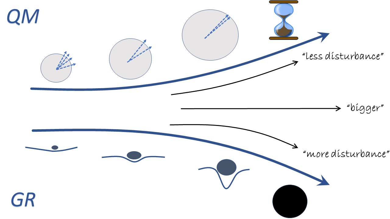
Figure 1: Fundamental limits on clocks. Detailed studies on models for quantum clocks indicate that, as is typically the case in quantum systems, relative uncertainties decrease with the energy of the system. However, increasing the energetic content comes at a cost, since general relativity effects start to play a role. Ultimately, the maximum energy that can be stored within a region is bounded, given that once the system becomes a black hole no information can be retrieved, and the system becomes useless as a clock. Phenomenological analyses combining these arguments have been used to derive fundamental limits on the accuracy with which time and length intervals can be measured.

Admittedly, the heuristic arguments used to derive $\Delta_{T}$ and $\Delta_{L}$ might not end up being exact in the light of a theory combining quantum mechanics and general relativity. Nevertheless, while we use (16) in the remainder of the paper, we note that the exact scaling with $T$ and $L$ will not be particularly relevant for the qualitative subsequent conclusions.

These fundamental uncertainties influence physics. Indeed, since the ideal parameter $t$ is inaccessible, it is unphysical to express the evolution of what can be observed of a system in terms of it. Instead, the physically meaningful approach is to express physics relationally, solely in terms of observable quantities.

In order to model this we consider a physical device used to track time. i.e. a clock, with a dynamics dictated by a Hamiltonian $H_{\mathcal{C}}$, that for simplicity we assume evolves independently from the system of interest (in this case $\mathcal{S}+\mathcal{E}$) with a Hamiltonian $H$. Then, the full Hamiltonian of $\mathcal{S}+\mathcal{E}+\mathcal{C}$ is

$$H_{\textnormal{total}}=H\otimes\mathbbm{1}_{\mathcal{C}}+\mathbbm{1}_{\mathcal{S}\mathcal{E}}\otimes H_{\mathcal{C}}.$$ (17)

Hence, given an initially uncorrelated clock the full state evolves according to

$$\rho_{\textnormal{total}}(t) =e^{-iH_{\textnormal{total}}t/\hbar}\rho_{\mathcal{S}\mathcal{E}}(0)\otimes\rho_{\mathcal{C}}(0)e^{iH_{\textnormal{total}}t/\hbar}$$

$$=e^{-iHt/\hbar}\rho_{\mathcal{S}\mathcal{E}}(0)e^{iHt/\hbar}\otimes e^{-iH_{\mathcal{C}}t/\hbar}\rho_{\mathcal{C}}(0)e^{iH_{\mathcal{C}}t/\hbar}$$

$$=\rho_{\mathcal{S}\mathcal{E}}(t)\otimes\rho_{\mathcal{C}}(t).$$ (18)

In order for the clock to act as such, some observable

$$\hat{T}=\sum_{T}T\hat{\Pi}_{T}$$ (19)

has to be a reliable time-tracking observable, where $\hat{\Pi}_{T}$ is a projector onto the subspace corresponding to eigenvalue $T$ of $\hat{T}$. That is, the evolution of $\operatorname{Tr}\left[{\hat{T}\rho_{\mathcal{C}}(t)}\right]$ should track the ideal time $t$. Then, a meaningful way to describe the dynamics of an observable $\hat{O}=\sum_{O}O\hat{\Pi}_{O}$ is to consider the conditional probability of observing a particular value $O$ given that the physical time takes a value $T$. Such conditional probability is given by

$$\mathcal{P}(O|T)=\lim_{t_{0}\to\infty}\frac{\displaystyle\int_{-t_{0}}^{t_{0}}\text{Tr}\Big{[}P_{O}P_{T}\rho_{\mathcal{S}\mathcal{E}}(t)P_{T}\Big{]}dt}{\displaystyle\int_{-t_{0}}^{t_{0}}\text{Tr}\Big{[}P_{T}\rho_{\mathcal{S}\mathcal{E}}(t)\Big{]}dt},$$ (20)

where the unobservable parameter $t$ is integrated over Gambini et al. (2007, 2009).

The approach followed here is naturally geared towards a relational description of the world, like the one provided by general relativity. Our approach would work even in a description where time is an emergent property of the universe. Page and Wootters Page and Wootters (1983) pioneered the use of a relational time in general relativity and some shortcomings of their approach were addressed in Gambini et al. (2009).

Interestingly, the traditional rule for calculating probabilities is recovered,

$$\mathcal{P}(O|T) =\text{Tr}\bigg{(}P_{O}\int\rho_{\mathcal{S}\mathcal{E}}(t)\mathcal{P}_{t}(T)dt\bigg{)}$$

$$\equiv\text{Tr}\big{(}P_{O}\rho_{\mathcal{S}\mathcal{E}}(T)\big{)},$$ (21)

where with some abuse of notation we denote

$$\rho_{\mathcal{S}\mathcal{E}}(T)\equiv\int\rho_{\mathcal{S}\mathcal{E}}(t)\mathcal{P}_{t}(T)dt,$$ (22)

and

$$\mathcal{P}_{t}(T)\equiv\frac{\text{Tr}\big{[}P_{T}\rho_{\mathcal{C}}(t)\big{]}}{\lim_{t_{0}\to\infty}\int_{-t_{0}}^{t_{0}}\text{Tr}\big{[}P_{T}\rho_{\mathcal{C}}(t)\big{]}dt}$$ (23)

is the probability of getting $T$ at the ideal time $t$. The effective state $\rho_{\mathcal{S}\mathcal{E}}(T)$ then gives a characterization of the observable physics in terms of the physical time $T$.

With access to an ideal clock, for which ${P}_{t}(T)=\delta(T-t)$, one immediately recovers the traditional quantum mechanical result. However, fundamental time uncertainties lead to non-unitary evolution. Here is a simple way to illustrate it. Consider, for simplicity, that the clock is characterized by a Gaussian distribution centered around the ideal time value $t$, with a standard deviation given by the fundamental uncertainty on measuring time intervals. That is, assume

$$\mathcal{P}_{t}(T)=\frac{1}{\sqrt{2\pi\Delta_{T}^{2}}}e^{-\frac{(T-t)^{2}}{2\Delta_{T}^{2}}},$$ (24)

where $\Delta_{T}=T_{P}^{2/3}T^{1/3}$. Expressing the initial density matrix in the energy eigenbasis as

$$\rho_{\mathcal{S}\mathcal{E}}(0)=\sum_{nm}\rho_{nm}\left|n\right\rangle\!\vphantom{\left(n\right)^{A}}\left\langle m\right|\vphantom{\left(m\right)^{A}},\qquad H=\sum_{n}E_{n}\left|n\right\rangle\!\vphantom{\left(n\right)^{A}}\left\langle n\right|\vphantom{\left(n\right)^{A}},$$ (25)

the evolution in terms of ideal time $t$ is given by

$$\rho_{\mathcal{S}\mathcal{E}}(t)=\sum_{nm}\rho_{nm}e^{-i(E_{n}-E_{m})t/\hbar}\left|n\right\rangle\!\vphantom{\left(n\right)^{A}}\left\langle m\right|\vphantom{\left(m\right)^{A}}.$$ (26)

From here the evolution in terms of a physical time then becomes

$$\rho_{\mathcal{S}\mathcal{E}}(T) = \sum_{nm}\rho_{nm}e^{-i(E_{n}-E_{m})T/\hbar}$$ (27)

$$\times e^{-(E_{n}-E_{m})^{2}\Delta_{T}^{2}/(2\hbar^{2})}\left|n\right\rangle\!\vphantom{\left(n\right)^{A}}\left\langle m\right|\vphantom{\left(m\right)^{A}}.$$

Note that it can be decomposed into unitary and non-unitary parts:

$$\rho_{\mathcal{S}\mathcal{E}}(T)=e^{-iHT/\hbar}\Omega_{T}(\rho_{\mathcal{S}\mathcal{E}}(0))e^{iHT/\hbar},$$ (28)

where the map $\Omega_{T}$ is defined by

$$\Omega_{T}(\left|n\right\rangle\!\vphantom{\left(n\right)^{A}}\left\langle m\right|\vphantom{\left(m\right)^{A}}\!)=\sum_{nm}e^{-(E_{n}-E_{m})^{2}\Delta_{T}^{2}/(2\hbar^{2})}\left|n\right\rangle\!\vphantom{\left(n\right)^{A}}\left\langle m\right|\vphantom{\left(m\right)^{A}}.$$ (29)

The physically accessible density matrix $\rho_{\mathcal{S}\mathcal{E}}(T)$ then evolves according to the master equation

$$\frac{\partial\rho_{\mathcal{S}\mathcal{E}}(T)}{\partial T} = -\frac{i}{\hbar}[H,\rho_{\mathcal{S}\mathcal{E}}(T)]$$ (30)

$$-\frac{1}{2\hbar^{2}}\frac{\partial(\Delta_{T}^{2})}{\partial T}\left[H,[H,\rho_{\mathcal{S}\mathcal{E}}(T)]\right].$$

While the first term corresponds to unitary quantum theory, the second term induces a loss of coherence in the energy basis, strictly due to the fundamental time uncertainties. In Gambini et al. (2007) it is shown that for short times the effective state undergoes such non-unitary dynamics without the assumption of a Gaussian distribution for the clock. Note that similar evolutions have been considered in the literature, with different motivations Milburn (1991); Egusquiza et al. (1999); Diósi (2005). Here the crucial point is that, under the assumption that ideal time measurements are forbidden in nature, such non-unitary evolution is fundamental. Any system described relationally is inevitably bound by these limits, and its evolutions will be described by the master equation (30). Note, too, that the above analysis can be extended to include decoherence due to errors in measuring length scales in quantum field theory. As such, even if we present our results within non-relativistic quantum mechanics, they are naturally geared towards covariant formulations of quantum theory Gambini et al. (2006).

A question that naturally arises at this point is whether enlarging the analysis to include the clock system could change the results, i.e. how fundamental is this process, when it depends on the clock system? While our description explicitly includes a physical device used as clock, such loss of coherence is inescapable. Imagine the set of all physical processes in the universe that can serve to track time. If fundamental uncertainties exist, all such processes will be restricted by them. Then, the best one could aim for when describing another physical process is having such optimal clock in hand, as we have done above. Any realistic setting, with a realistic clock, will at least suffer from the above loss of coherence.

IV Production of events

Let us analyze the global protocol introduced in Sec. II in terms of the fundamentally non-unitary evolution of the total closed system $\mathcal{S}+\mathcal{E}$ due to formulating physics in terms of a measurable time $T$. First, note that in the best case scenario the global unitary $U$ undoes the unitary part of the evolution in Eq. (28) given a previous timespan $T$. Then, the final state expressed in terms of a physical time $T$ is

$$\rho_{\mathcal{S}\mathcal{E}}(T_{f})=\sum_{nm}\rho_{nm}e^{-(E_{n}-E_{m})^{2}\Delta_{2T}^{2}/(2\hbar^{2})}\left|n\right\rangle\!\vphantom{\left(n\right)^{A}}\left\langle m\right|\vphantom{\left(m\right)^{A}},$$ (31)

where we are assuming implementation of the unitary $U$ by a time-reversal operation during a time $T$, resulting in a total time $2T$ over which loss of coherence occurs.

Using the fact that $e^{-(E_{n}-E_{m})^{2}\Delta_{2T}^{2}/(2\hbar^{2})}=\sqrt{\frac{1}{2\pi\Delta_{T}^{2}}}\int_{-\infty}^{\infty}e^{-\mu^{2}/(2\Delta_{2T}^{2})}e^{-i(E_{n}-E_{m})\mu/\hbar}d\mu$, the final state can be expressed as

$$\rho_{\mathcal{S}\mathcal{E}}(T_{f}) =\sum_{nm}\rho_{nm}\sqrt{\frac{1}{2\pi\Delta_{2T}^{2}}}$$

$$\int_{-\infty}^{\infty}e^{-\mu^{2}/(2\Delta_{2T}^{2})}e^{-i(E_{n}-E_{m})\mu/\hbar}d\mu\left|n\right\rangle\!\vphantom{\left(n\right)^{A}}\left\langle m\right|\vphantom{\left(m\right)^{A}}$$

$$=\sqrt{\frac{1}{2\pi\Delta_{2T}^{2}}}\int_{-\infty}^{\infty}e^{-\mu^{2}/(2\Delta_{2T}^{2})}\widetilde{\rho}_{\mathcal{S}\mathcal{E}}(\mu)d\mu,$$ (32)

where $\widetilde{\rho}_{\mathcal{S}\mathcal{E}}(\mu)\equiv e^{-iH\mu}\rho_{\mathcal{S}\mathcal{E}}(0)e^{iH\mu}$ is the unitarily evolved state (in order to avoid confusion in this section we distinguish it from the effective state at a physical time $T$ by a tilde). Similarly,

$$\rho_{\mathcal{S}\mathcal{E}}^{\text{event}}(T_{f}) =\sqrt{\frac{1}{2\pi\Delta_{2T}^{2}}}\int_{-\infty}^{\infty}e^{-\mu^{2}/(2\Delta_{2T}^{2})}\widetilde{\rho}_{\mathcal{S}\mathcal{E}}{}^{\text{event}}(\mu)d\mu.$$ (33)

The unitary evolution of system plus environment was analyzed in Section I. From Eq. (I) we obtain that for an observable $O=O_{\mathcal{S}}\otimes\mathbbm{1}_{\mathcal{E}}$:

$$\operatorname{Tr}\left[{O\big{(}\rho_{\mathcal{S}\mathcal{E}}(T_{f})-\rho_{\mathcal{S}\mathcal{E}}^{\text{event}}(T_{f})\big{)}}\right]$$

$$=\sqrt{\frac{1}{2\pi\Delta_{2T}^{2}}}\int_{-\infty}^{\infty}e^{-\mu^{2}/(2\Delta_{2T}^{2})}\operatorname{Tr}\left[{O\big{(}\widetilde{\rho}_{\mathcal{S}\mathcal{E}}(\mu)-\widetilde{\rho}_{\mathcal{S}\mathcal{E}}^{\text{event}}(\mu)\big{)}}\right]d\mu$$

$$=\sqrt{\frac{1}{2\pi\Delta_{2T}^{2}}}\int_{-\infty}^{\infty}e^{-\mu^{2}/(2\Delta_{2T}^{2})}d\mu$$

$$\qquad\sum_{j\neq k}\alpha_{j}\alpha_{k}^{*}\operatorname{Tr}\left[{O_{S}\left|\varphi_{j}\right\rangle\!\vphantom{\left(\varphi_{j}\right)^{A}}\!\left\langle\varphi_{k}\right|\vphantom{\left(\varphi_{k}\right)^{A}}}\right]\left\langle E_{j}(\mu)\right|\vphantom{\left(E_{j}(\mu)\right)^{A}}E_{k}(\mu)\rangle.$$ (34)

For a great number of decoherence models the overlap between the environmental states decays exponentially Schlosshauer (2014), in which case

$$\operatorname{Tr}\left[{O\big{(}\rho_{\mathcal{S}\mathcal{E}}(T_{f})-\rho_{\mathcal{S}\mathcal{E}}^{\text{event}}(T_{f})\big{)}}\right]\approx$$

$$\qquad\sqrt{\frac{1}{2\pi\Delta_{2T}^{2}}}\int_{-\infty}^{\infty}e^{-\mu^{2}/(2\Delta_{2T}^{2})}e^{-|\mu|/\tau_{D}}d\mu$$

$$\qquad\quad\qquad\sum_{j\neq k}\alpha_{j}\alpha_{k}^{*}\operatorname{Tr}\left[{O_{S}\left|\varphi_{j}\right\rangle\!\vphantom{\left(\varphi_{j}\right)^{A}}\!\left\langle\varphi_{k}\right|\vphantom{\left(\varphi_{k}\right)^{A}}}\right]\left\langle E_{j}(0)\right|\vphantom{\left(E_{j}(0)\right)^{A}}E_{k}(0)\rangle$$

$$=e^{\Delta_{2T}^{2}/2\tau_{D}^{2}}\,\text{erfc}\left(\frac{\Delta_{2T}}{\sqrt{2}\tau_{D}}\right)\operatorname{Tr}\left[{O\big{(}\rho_{\mathcal{S}\mathcal{E}}(0)-\rho_{\mathcal{S}\mathcal{E}}^{\text{event}}(0)\big{)}}\right]$$

$$\qquad\leq\frac{\sqrt{2}\tau_{D}}{\sqrt{\pi}\Delta_{2T}}\operatorname{Tr}\left[{O_{\mathcal{S}}\big{(}\rho_{\mathcal{S}}(0)-\rho_{\mathcal{S}}^{\text{event}}(0)\big{)}}\right],$$ (35)

where we used in the last step that the environment and system are not correlated initially.

Given Eqs. (16) as an estimate for the error in the physical time, we obtain

$$\operatorname{Tr}\left[{O\big{(}\rho_{\mathcal{S}\mathcal{E}}(T_{f})-\rho_{\mathcal{S}\mathcal{E}}^{\text{event}}(T_{f})\big{)}}\right]$$

$$\qquad\lesssim\frac{\sqrt{2}\tau_{D}}{\sqrt{\pi}2^{1/3}T_{P}^{2/3}T^{1/3}}\operatorname{Tr}\left[{O_{\mathcal{S}}\big{(}\rho_{\mathcal{S}}(0)-\rho_{\mathcal{S}}^{\text{event}}(0)\big{)}}\right].$$ (36)

This shows that using the global protocol to distinguish the evolved state from the state in case of an event becomes increasingly harder when time uncertainties are taken into account. The state thus becomes physically increasingly similar to the case in which an event occurs and it can be interpreted as a classical mixture.

V A fundamental criterion for the production of events

While distinguishing between $\rho_{\mathcal{S}\mathcal{E}}(0)$ and $\rho_{\mathcal{S}\mathcal{E}}^{\text{event}}(0)$ becomes increasingly hard when taking into account the loss of coherence due to uncertainties in time measurements, this is still a solution that works ‘for all practical purposes’ at this stage, given that in principle extremely precise measurements could distinguish them. We now show that this is not the case when one takes into account uncertainties on length measurements. We illustrate it in the paradigmatic case of a particle in a coherent superposition over two spatial locations.

For concreteness, consider that the initial state of the system is a 1-D coherent spatial superposition of Gaussian wavepackets of width $\sigma$ separated by a distance $L$:

$$\rho_{\mathcal{S}}(0) =|a|^{2}\left|\varphi_{1}\right\rangle\!\vphantom{\left(\varphi_{1}\right)^{A}}\!\left\langle\varphi_{1}\right|\vphantom{\left(\varphi_{1}\right)^{A}}+|b|^{2}\left|\varphi_{2}\right\rangle\!\vphantom{\left(\varphi_{2}\right)^{A}}\!\left\langle\varphi_{2}\right|\vphantom{\left(\varphi_{2}\right)^{A}}$$

$$+ab^{*}\left|\varphi_{1}\right\rangle\!\vphantom{\left(\varphi_{1}\right)^{A}}\!\left\langle\varphi_{2}\right|\vphantom{\left(\varphi_{2}\right)^{A}}+a^{*}b\left|\varphi_{2}\right\rangle\!\vphantom{\left(\varphi_{2}\right)^{A}}\!\left\langle\varphi_{1}\right|\vphantom{\left(\varphi_{1}\right)^{A}},$$ (37)

with

$$\langle x\left|\varphi_{1}\right\rangle\!\vphantom{\left(\varphi_{1}\right)^{A}} =\frac{1}{(2\pi\sigma^{2})^{1/4}}\exp\left(-\frac{(x-L/2)^{2}}{4\sigma^{2}}\right)$$ (38)

$$\langle x\left|\varphi_{2}\right\rangle\!\vphantom{\left(\varphi_{2}\right)^{A}} =\frac{1}{(2\pi\sigma^{2})^{1/4}}\exp\left(-\frac{(x+L/2)^{2}}{4\sigma^{2}}\right).$$ (39)

The corresponding state given the occurrence of an event on position is

$$\rho_{\mathcal{S}}^{\text{event}}(0) =|a|^{2}\left|\varphi_{1}\right\rangle\!\vphantom{\left(\varphi_{1}\right)^{A}}\!\left\langle\varphi_{1}\right|\vphantom{\left(\varphi_{1}\right)^{A}}+|b|^{2}\left|\varphi_{2}\right\rangle\!\vphantom{\left(\varphi_{2}\right)^{A}}\!\left\langle\varphi_{2}\right|\vphantom{\left(\varphi_{2}\right)^{A}}.$$ (40)

(Note that, while $\left|\varphi_{1}\right\rangle\!\vphantom{\left(\varphi_{1}\right)^{A}}$ and $\left|\varphi_{2}\right\rangle\!\vphantom{\left(\varphi_{2}\right)^{A}}$ are not orthonormal, their overlap is small as long as $L\gg\sigma$.)

Choosing the momentum operator $O_{S}=p$ can serve to distinguish between a coherent superposition and a statistical mixture over different spatial positions. Indeed, given that

$$\left\langle\varphi_{1}\right|\vphantom{\left(\varphi_{1}\right)^{A}}p\left|\varphi_{1}\right\rangle\!\vphantom{\left(\varphi_{1}\right)^{A}}=\left\langle\varphi_{2}\right|\vphantom{\left(\varphi_{2}\right)^{A}}p\left|\varphi_{2}\right\rangle\!\vphantom{\left(\varphi_{2}\right)^{A}}=0,$$ (41)

we have

$$\operatorname{Tr}\left[{p\rho_{\mathcal{S}}^{\text{event}}(0)}\right]=0.$$ (42)

Meanwhile, using that

$$\left\langle\varphi_{2}\right|\vphantom{\left(\varphi_{2}\right)^{A}}p\left|\varphi_{1}\right\rangle\!\vphantom{\left(\varphi_{1}\right)^{A}}=$$

$$\frac{-i\hbar}{\sqrt{2\pi\sigma^{2}}}\int\frac{-2(x-L/2)}{4\sigma^{2}}$$

$$\times\exp\left(-\frac{(x+L/2)^{2}+(x-L/2)^{2}}{4\sigma^{2}}\right)dx$$

$$\qquad=\frac{2i\hbar}{\sqrt{2\pi\sigma^{2}}}\int u\exp\left(-u^{2}-\left(u+\frac{L}{2\sigma}\right)^{2}\right)du$$

$$\qquad=-i\hbar\frac{L}{4\sigma^{2}}\exp\left(-\frac{L^{2}}{8\sigma^{2}}\right),$$ (43)

gives

$$\operatorname{Tr}\left[{p\rho_{\mathcal{S}}(0)}\right]=-i(ab^{*}-a^{*}b)\hbar\frac{L}{4\sigma^{2}}\exp\left(-\frac{L^{2}}{8\sigma^{2}}\right).$$ (44)

Hence, if the initial state is chosen with the appropriate phases, $p$ discriminates whether an event occurred or not.

Note, however, that fundamental uncertainties on the measurement of length intervals forbid a perfect preparation of the wavepackets $\left|\varphi_{1}\right\rangle\!\vphantom{\left(\varphi_{1}\right)^{A}}$ and $\left|\varphi_{2}\right\rangle\!\vphantom{\left(\varphi_{2}\right)^{A}}$, since they imply errors $\Delta L$ and $\Delta\sigma$ on the separation and width of the lobes. This in turn translates into uncertainties on the expectation value of $p$. A simple propagation of uncertainty on the error induced in $\operatorname{Tr}\left[{p\rho_{\mathcal{S}}(0)}\right]~{}-~{}\operatorname{Tr}\left[{p\rho_{\mathcal{S}}^{\text{event}}(0)}\right]$ gives

$$\Delta^{2}\left(\operatorname{Tr}\left[{p\rho_{\mathcal{S}}(0)}\right]-\operatorname{Tr}\left[{p\rho_{\mathcal{S}}^{\text{event}}(0)}\right]\right)$$

$$\quad=\left(\frac{\partial}{\partial L}\operatorname{Tr}\left[{p\rho_{\mathcal{S}}(0)}\right]\right)^{2}\Delta L^{2}+\left(\frac{\partial}{\partial\sigma}\operatorname{Tr}\left[{p\rho_{\mathcal{S}}(0)}\right]\right)^{2}\Delta\sigma^{2}$$

$$\quad=\left(\left(\frac{1}{L}-\frac{L}{4\sigma^{2}}\right)\operatorname{Tr}\left[{p\rho_{\mathcal{S}}(0)}\right]\right)^{2}\Delta L^{2}$$

$$\quad+\left(\left(-\frac{2}{\sigma}+\frac{L^{2}}{4\sigma^{3}}\right)\operatorname{Tr}\left[{p\rho_{\mathcal{S}}(0)}\right]\right)^{2}\Delta\sigma^{2}.$$ (45)

Expressing the standard deviation of the Gaussians as $\sigma=\epsilon L$, we get

$$\Delta^{2}\left(\operatorname{Tr}\left[{p\rho_{\mathcal{S}}(0)}\right]-\operatorname{Tr}\left[{p\rho_{\mathcal{S}}^{\text{event}}(0)}\right]\right)$$

$$\quad=\left(1-\frac{1}{4\epsilon^{2}}\right)^{2}\operatorname{Tr}\left[{p\rho_{\mathcal{S}}(0)}\right]^{2}\frac{\Delta L^{2}}{L^{2}}$$

$$\quad+\left(-\frac{2}{\epsilon}+\frac{1}{4\epsilon^{3}}\right)^{2}\operatorname{Tr}\left[{p\rho_{\mathcal{S}}(0)}\right]^{2}\epsilon^{2}\frac{\Delta L^{2}}{L^{2}}$$

$$\quad=\left(5-\frac{1}{\epsilon}-\frac{7}{16\epsilon^{2}}+\frac{1}{16\epsilon^{4}}\right)\operatorname{Tr}\left[{p\rho_{\mathcal{S}}(0)}\right]^{2}\frac{\Delta L^{2}}{L^{2}}$$

$$\quad\geq 2\operatorname{Tr}\left[{p\rho_{\mathcal{S}}(0)}\right]^{2}\frac{\Delta L^{2}}{L^{2}},$$ (46)

with the inequality valid for any choice of $\epsilon\geq 0$.

The uncertainty on the measurement of $O=p\otimes\mathbbm{1}_{\mathcal{E}}$ has to be taken into account when analyzing the global protocol considered in the previous section. Once the condition

$$\operatorname{Tr}\left[{p\big{(}\rho_{\mathcal{S}\mathcal{E}}(T_{f})-\rho_{\mathcal{S}\mathcal{E}}^{\text{event}}(T_{f})\big{)}}\right]$$

$$\qquad\quad\leq\Delta\left(\operatorname{Tr}\left[{p\left(\rho_{\mathcal{S}}(0)-\rho_{\mathcal{S}}^{\text{event}}(0)\right)}\right]\right)$$ (47)

is satisfied, the uncertainty in the measurement of the observable prevents one from verifying whether the system is in a coherent superposition $\rho_{\mathcal{S}\mathcal{E}}(0)$ or in a statistical mixture $\rho_{\mathcal{S}\mathcal{E}}^{\text{event}}(0)$, as illustrated in Fig. 2. Given the last bound on Eq. (V), this eventually happens for large enough $T_{f}$. Notice that this is a fundamental limitation and cannot be circumvented by making multiple measurements. It is related to the impossibility of preparing exactly the same initial state with infinite precision. This is an explicit implementation of the notion of undecidability between a mixture state and one resulting from the evolution that, with an example of a spin system, was used in formulating the Montevideo Interpretation of quantum mechanics Gambini et al. (2010, 2011a).

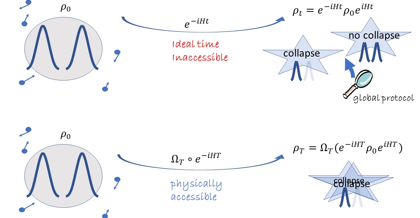
Figure 2: Production of events. (Top) Within ordinary unitary quantum theory, there exists global protocols, i.e. unitary operations followed by measurements, that allow to distinguish the unitarily evolved state from the state one would have if an event, or collapse, had occurred. Thus, the final state cannot be interpreted as a classical probability distribution over the set of pointer states. In the example shown, a definite position for the particle cannot be assigned. (Bottom) However, when the loss of coherence due to uncertainties in time measurements is taken into consideration, the power of these global protocols to distinguish the two situations is diminished. After a long enough period of time has passed, fundamental uncertainties in the initial state of the system, in this example related to the initial position of the particle, forbid one from physically distinguishing the evolved state from a state where the particle ends up in a definite position, with a certain probability. In such situations, when the state is physically completely indistinguishable from a classically interpretable state (statistical mixture), we say that an event has occurred.

In order to estimate how fast one arrives at the condition described by equation (47), we focus on a particular decoherence model. In the past our attention went to models of decoherence on a spin degree of freedom, so for completeness we now analyze decoherence of spatial superpositions due to a scattering processes with an environment (see for example Chapter 3 of Schlosshauer (2007) for a detailed presentation). Adopting the terminology of that presentation, for a “central system” $\mathcal{S}$ of mass $M$ and cross-section $a$ undergoing scattering events with a bath of smaller particles, a spatial superposition over a distance $L$ exponentially decays on a timescale

$$\tau_{D}=\frac{1}{\Lambda L^{2}},$$ (48)

where

$$\Lambda=\frac{\sqrt{2\pi}8}{3\hbar^{2}}\nu\sqrt{M}a^{2}(K_{B}\text{Temp})^{3/2}$$ (49)

is the scattering constant, and depends on characteristics of central system, the environment, and the interaction between them. Here, $\nu$ is the density of particles in the environment of temperature Temp, and $K_{B}$ is Boltzmann’s constant. Schlosshauer gives a detailed treatment of the decoherence timescales of different central systems, and in the presence of a variety of baths. For instance, an atomic-sized dust grain ($a\sim 10^{-8}m$) initially in a superposition over $L=a$ is decohered by air at room temperature and normal pressure ($\nu\approx 3\times 10^{23}m^{-3}$) on a timescale $\tau_{D}\sim 10^{-31}s$.

For illustration purposes we follow Schlosshauer, and take superpositions over distances of the order of the size of the central system, $L=a$. Combining Eqs. (16), (IV) and (V), we conclude that an event occurs for times $T>\tau_{\text{event}}$, where the event time $\tau_{\text{event}}$ satisfies

$$\frac{\sqrt{2}\tau_{D}}{\sqrt{\pi}2^{1/3}T_{P}^{2/3}\tau_{\text{event}}^{1/3}}=\frac{\sqrt{2}\Delta L}{L}=\frac{\sqrt{2}L_{P}^{2/3}}{L^{2/3}}.$$ (50)

That is, for times $T>\tau_{\text{event}}$, fundamental uncertainties on time and length intervals prevent one from distinguishing $\rho_{\mathcal{S}\mathcal{E}}$ from $\rho_{\mathcal{S}\mathcal{E}}^{\text{event}}$ with global protocols, where

$$\tau_{\text{event}}=\frac{1}{2(2\pi)^{3/2}}\frac{\tau_{D}^{3}L^{2}}{T_{P}^{2}L_{P}^{2}}.$$ (51)

From then on, physical predictions are exactly as if the system is found in a statistical mixture.

The event timescale can be evaluated for different central systems. For an atomic-sized dust grain ($a\sim 10^{-8}m$) this is still an extremely large timescale, $\tau_{\text{event}}\sim 1\times 10^{44}s$, i.e. no event occurs within the lifetime of the universe. However, for a larger particle of the same mass density as a dust grain and characteristic size $a\sim 10^{-5}m$ the estimate of the event timescale becomes $\tau_{\text{event}}\sim 50s$, while for one of characteristic size $a\sim 10^{-4}m$ events happen extremely quickly, within $\tau_{\text{event}}\sim 10^{-12}s$. Such estimates are readily derived from eqs. (48), (49) and (51) by noting that scaling the characteristic length of the particle by a factor $\alpha$ decreases the event time by a factor $\alpha^{-29/2}$. Remarkably, the quantum/classical boundary is set on the verge of the macroscopic scale, from this simple analysis. Naturally, a more realistic analysis could shift this line, as would a change in the fundamental time and length uncertainties. However, given the dependence of $\tau_{\text{event}}$ on the environmental decoherence timescales $\tau_{D}$, and the remarkable short values of the latter for big systems, events will invariably occur for macroscopic systems. Note that detailed previous analysis on spin-spin decoherence models show that more stringent timescales for events can occur in other cases Gambini et al. (2010, 2011a).

VI A consistent single-world interpretation of quantum mechanics

Frauchiger and Renner recently showed that no “single-world” interpretation of quantum mechanics can be self-consistent Frauchiger and Renner (2018) (for accessible colloquial and pedagogical presentations see Pusey (2018); Araújo (2016); Nurgalieva and del Rio (2018)). That is, if quantum mechanics exactly describes complex systems like the observers and their measuring devices, one needs to either give up “the view that there is a single reality”, or the expectation of consistency between observations of different agents. A single-world interpretation is any interpretation that asserts, for a quantum measurement with multiple possible outcomes, that just one outcome and its corresponding reduction of the state actually occurs.

More precisely, they proved that the three following conditions are incompatible: (Q) – the theory is described by standard quantum mechanics. This includes the use of the Born rule to predict that certain outcomes occur with probability one. This condition also presumes ideal, unitary, quantum theory (if only an implicit assumption in their work Nurgalieva and del Rio (2018)); (C) – the theory is self-consistent. By this, one assumes that predictions done by independent agents agree with each other; (S) – the theory corresponds to a single-world description, where each agent only observes a single outcome in a measurement.

To prove the theorem, they consider two observers Alice and Bob that perform measurements in their labs $S_{A}$ and $S_{B}$. The measurements of Bob depend on the outcomes observed by Alice. The measured quantum systems, as well as Alice and Bob, their measuring instruments and all the systems in their laboratories that become entangled with the measuring instruments in registering and recording the outcomes of the quantum measurements, including the entangled environments, are just two big many-body quantum systems $S_{A}$ and $S_{B}$, which are assumed to be completely isolated from each other after Bob receives Alice’s information. Consider two super-observers, Wigner and Friend, with vast technological abilities, who measure a super-observable X of $S_{A}$ and a super-observable Y of $S_{B}$.

As the evolution of $S_{A}$ and $S_{B}$ according to ordinary quantum mechanics is unitary (Q), the authors are able to show that, for a particular situation, there is no consistent story that includes observers and super-observers: a pair of outcomes with finite probability, according to quantum mechanics, of the super-observers’ measurements on the composite observer system is inconsistent with the observers obtaining definite (single) outcomes for their measurements. Note that their no-go theorem does not give a hint as to which of the three conditions, or extra implicit assumption Frauchiger and Renner (2018); Nurgalieva and del Rio (2018); Aaronson (2018), needs to be dropped.

Following Bub’s notation Bub (2018) the essence of the argument can be summarized as follows: while for Alice and Bob the final state after their measurements is given by a density matrix,

$$\rho = \frac{1}{3}|0\rangle_{B}|h\rangle_{A}\langle h|_{A}\langle 0|_{B}+\frac{1}{3}|0\rangle_{B}|t\rangle_{A}\langle t|_{A}\langle 0|_{B}$$ (52)

$$+\frac{1}{3}|1\rangle_{B}|t\rangle_{A}\langle t|_{A}\langle 1|_{B},$$

the super-observers, due to the unitary evolution, will assign a pure state for the complete system

$$|\psi\rangle=\frac{1}{\sqrt{3}}\left(|h\rangle_{A}|0\rangle_{B}+|t\rangle_{A}|0\rangle_{B}+|t\rangle_{A}|1\rangle_{B}\right).$$ (53)

Frauchiger and Renner prove that following the storyline of each of the agents involved leads to contradictions between their observations.

However, if we take into account the loss of unitarity due to time and length uncertainties, the final state for Alice, Bob and the super-observers will coincide and take the form (52). Therefore, subsequent measurements will not lead to any contradiction. As a matter of fact, since our definition of event rests on the fact that there are instances in which the state becomes physically identical to a classical probability distribution, as in (52), the picture put forward is thus as consistent as classical probability theory.

The approach that we have presented here may be also viewed as the way of making quantum mechanics compatible with a consistent single-world interpretation by including the loss of unitarity induced by fundamental limitations on the measurement of time and length. The inclusion of such limitations due to quantum and gravitational effects allows showing that, if one incorporates in quantum theory these effects and consider the corresponding theory (QG), then this extended theory satisfies the conditions (S) and (C) as well.

VII Discussion

Quantum theory involves a huge leap from the understanding of preceding theories, giving a central role to the act of measurement. This holds irrespective of the philosophical standpoint that one takes: physical predictions following a measurement are different than before the measurement Our view is that the understanding of quantum theory is not complete until a proper characterization of the process of measurement is at hand. One that unequivocally defines the process by which a quantum system undergoes the change

$$\rho_{\mathcal{S}}\Longrightarrow\rho_{\mathcal{S}}^{\text{event}},$$ (54)

that is, from a coherent superposition to a state that can be attributed definite outcomes. Environmental decoherence gets one very close to the above, identifying instances in which the transition occurs for all practical purposes. However, in our opinion these sort of solutions are not enough, since at best one ends up with a subjective, and fuzzy, notion of event. There are protocols that serve to flesh out the fact that the ‘decoherence solution’ is apparent. In particular, in this paper we consider a set of global protocols for which the predictions for $\rho_{\mathcal{S}}$ and $\rho_{\mathcal{S}}^{\text{event}}$ differ within unitary quantum mechanics.

Naturally, we are not alone in this criticism, and endless work has been devoted to different modifications and/or re-interpretations of the theory to attempt such understanding. Many of these attempts involve trade-offs, for example giving up the possibility of a single-world description in exchange for keeping the formalism of quantum theory intact Everett III (1957); DeWitt (1970); Saunders et al. (2010); Vaidman (2016), reinterpreting the existing theory by willing to lose the notion of objectivity Fuchs and Schack (2013); Fuchs et al. (2014), accepting ad-hoc modifications to quantum theory in order to restore a single-world picture Diósi (1984); Ghirardi et al. (1986); Diósi (1988); Pearle (1989); Ghirardi et al. (1990); Gisin (1989); Penrose (1996); Gisin (2017), or even a combination of all of the above Mueller (2017). While we see benefits to all of these approaches, here we attempt a construction of a realist description, with well defined notion of events, and with minimal, physically grounded, premises.

Our starting point is to assume that the laws of the universe do not allow for arbitrarily precise measurements. The argument behind this is simple. When one considers physical mechanisms that allow to measure a physical quantity, say time, one finds that quantum mechanics leads to uncertainties in such measurements. Typically, these uncertainties can be made small by designing systems that suffer less from quantum mechanical effects, for example by increasing energy and/or size. However, this procedure clashes with general relativity, which dictates limits on the energetic content within a region. Assuming that both of these general traits will survive in a fundamental theory that combines quantum mechanics and general relativity, one invariably ends up with fundamental uncertainties. These minuscule errors on the measurement of time and length intervals can have far reaching consequences on what one can interpret quantum theory to be about.

Fundamental uncertainties in time lead to a loss of coherence in the energy basis. In this paper we proved that this loss of coherence is enough to rule out a large set of global protocols that allow to verify that no objective event occurs within unitary quantum theory. In our approach, these instances, in which the predictions become indistinguishable to the case in which the system is in a classically interpretable state, are the events. As such, we paint a picture with a clear cut definition of when events take place and when they do not, on a pointer basis determined by the interplay of the different Hamiltonians involved in the problem, and with a well defined timescale, for which we gave estimates in a paradigmatic model of a particle delocalized in space. Note, in particular, that our notion of event needs no reference to observers. The condition for the event to happen or not is uniquely defined by the state of the system, and the limits that nature imposes on measurements. The events defined in this way completely characterize the physical quantities of the system, and possibly the environment, that take definite values Gambini et al. (2011b).

Summarizing, the previous analysis suggests the following ontology: the classical world is composed by of events. An event takes place when the state of a closed system, -i.e a system for which its state gives a complete description- takes the form of a statistical mixture. Most states that quantum systems can be found in, in particular coherent superpositions over sets of states, only describe potentialities to produce events. On the other hand, statistical mixtures of closed systems are classically interpretable states. These states can be thought of as a classical statistical mixture of states corresponding to different outcomes. Quantum mechanics provides the probabilities for these, that occur randomly. It has no information about which of the possible outcome has occurred. When this condition is satisfied we know that an event occurred but we ignore which one it was. The collapse of the wave function when an event is observed is nothing but the actualization of the information that we posses about events that have already occurred.

At this point one would naturally ask: “isn’t the and/or problem still present?”. That is, have we adequately explained the transition from a superposition to a single outcome? We believe this to no longer be a problem once all physical predictions are as is the system is described by a classical probability distribution. If from the beginnings of quantum theory the founding fathers had found that there are instances in which a quantum system is describable by classical probability distributions, then the and/or question would have never arisen, the same way it doesn’t come up when tossing a coin.

Note that this is not simply a philosophical re-interpretation of quantum theory. Our predictions are testable, and the Montevideo Interpretation is falsifiable. Should experiments searching for deviations from unitary evolution rule out the fundamental loss of coherence introduced in Sec. III, or ever more precise clocks were conceived, then our approach would be proven wrong Fröwis et al. (2018). Modifications of experiments such as Vinante et al. (2017) to probe decoherence in energy would thus be extremely interesting.

Acknowledgments — This work was supported in part by Grant No. NSF-PHY-1603630, funds of the Hearne Institute for Theoretical Physics, CCT-LSU, and Pedeciba and Fondo Clemente Estable FCE_1_2014_1_103803, and the John Templeton Foundation.

References

- Spekkens (2007) R. W. Spekkens, “Evidence for the epistemic view of quantum states: A toy theory,” Phys. Rev. A 75, 032110 (2007), quant-ph/0401052 .
- Leifer (2014) M. Leifer, “Is the quantum state real? an extended review of -ontology theorems,” Quanta 3, 67–155 (2014).
- Gambini et al. (2010) R. Gambini, L. P. G. Pintos, and J. Pullin, “Undecidability and the Problem of Outcomes in Quantum Measurements,” Foundations of Physics 40, 93–115 (2010), arXiv:0905.4222 [quant-ph] .
- Gambini et al. (2011a) R. Gambini, L. P. García-Pintos, and J. Pullin, “Undecidability as Solution to the Problem of Measurement:. Fundamental Criterion for the Production of Events,” International Journal of Modern Physics D 20, 909–918 (2011a), arXiv:1009.3817 [quant-ph] .
- Gambini and Pullin (2009) R. Gambini and J. Pullin, “The montevideo interpretation of quantum mechanics: frequently asked questions,” Journal of Physics: Conference Series 174, 012003 (2009).
- Gambini et al. (2011b) R. Gambini, L. P. García-Pintos, and J. Pullin, “An axiomatic formulation of the Montevideo interpretation of quantum mechanics,” Studies in the History and Philosophy of Modern Physics 42, 256–263 (2011b), arXiv:1002.4209 [quant-ph] .
- Gambini and Pullin (2018) R. Gambini and J. Pullin, “The montevideo interpretation of quantum mechanics: A short review,” Entropy 20 (2018).
- Zeh (1970) H. D. Zeh, “On the interpretation of measurement in quantum theory,” Foundations of Physics 1, 69–76 (1970).
- Paz and Zurek (1999) J. P. Paz and W. H. Zurek, “Quantum limit of decoherence: Environment induced superselection of energy eigenstates,” Phys. Rev. Lett. 82, 5181–5185 (1999).
- Schlosshauer (2005) M. Schlosshauer, “Decoherence, the measurement problem, and interpretations of quantum mechanics,” Rev. Mod. Phys. 76, 1267–1305 (2005).
- Schlosshauer (2014) M. Schlosshauer, “The quantum-to-classical transition and decoherence,” ArXiv e-prints (2014), arXiv:1404.2635 [quant-ph] .
- Zurek (1991) W. H. Zurek, “Decoherence and the transition from quantum to classical,” Physics today 44, 36–44 (1991).
- Zurek (2003) W. H. Zurek, “Decoherence, einselection, and the quantum origins of the classical,” Rev. Mod. Phys. 75, 715–775 (2003).
- Riedel and Zurek (2010) C. J. Riedel and W. H. Zurek, “Quantum darwinism in an everyday environment: Huge redundancy in scattered photons,” Physical review letters 105, 020404 (2010).
- Schlosshauer (2007) M. Schlosshauer, Decoherence: and the quantum-to-classical transition (Springer Science & Business Media, 2007).
- Joos et al. (2013) E. Joos, H. D. Zeh, C. Kiefer, D. J. W. Giulini, J. Kupsch, and I. Stamatescu, Decoherence and the appearance of a classical world in quantum theory (Springer Science & Business Media, 2013).
- Wigner (1967) E. P. Wigner, Symmetries and reflections: Scientific essays of Eugene P. Wigner (Indiana University Press Bloomington, 1967).
- d’Espagnat (1995) B. d’Espagnat, “Veiled reality an analysis of present-day quantum mechanical concepts,” (1995).
- Frauchiger and Renner (2018) D. Frauchiger and R. Renner, “Quantum theory cannot consistently describe the use of itself,” Nature Communications 9, 3711 (2018).
- Jalabert and Pastawski (2001) R. A. Jalabert and H. M. Pastawski, “Environment-independent decoherence rate in classically chaotic systems,” Phys. Rev. Lett. 86, 2490–2493 (2001).
- Petitjean and Jacquod (2006) C. Petitjean and Ph. Jacquod, “Quantum reversibility and echoes in interacting systems,” Phys. Rev. Lett. 97, 124103 (2006).
- Goussev et al. (2012) A. Goussev, R. A. Jalabert, H. M. Pastawski, and D. Ariel Wisniacki, “Loschmidt echo,” Scholarpedia 7, 11687 (2012), revision #127578.
- Peres (1984) A. Peres, “Stability of quantum motion in chaotic and regular systems,” Phys. Rev. A 30, 1610–1615 (1984).
- Navascués (2018) M. Navascués, “Resetting uncontrolled quantum systems,” Phys. Rev. X 8, 031008 (2018).
- Saunders et al. (2010) S. Saunders, J. Barrett, A. Kent, and D. Wallace, Many worlds?: Everett, quantum theory, & reality (Oxford University Press, 2010).
- Salecker and Wigner (1958) H. Salecker and E. P. Wigner, “Quantum limitations of the measurement of space-time distances,” Phys. Rev. 109, 571–577 (1958).
- Peres (1980) A. Peres, “Measurement of time by quantum clocks,” American Journal of Physics 48, 552–557 (1980).
- Peres (2006) A. Peres, Quantum theory: concepts and methods, Vol. 57 (Springer Science & Business Media, 2006).
- Aharonov et al. (1998) Y. Aharonov, J. Oppenheim, S. Popescu, B. Reznik, and W. G. Unruh, “Measurement of time of arrival in quantum mechanics,” Phys. Rev. A 57, 4130–4139 (1998).
- Bužek et al. (1999) V. Bužek, R. Derka, and S. Massar, “Optimal quantum clocks,” Phys. Rev. Lett. 82, 2207–2210 (1999).
- Muga et al. (2007) J. G. Muga, R. Sala Mayato, and I. L. Egusquiza, Time in Quantum Mechanics, Vol. 1 (Springer, Berlin, 2007).
- Muga et al. (2009) J. G. Muga, A. Ruschhaupt, and A. del Campo, Time in Quantum Mechanics, Vol. 2 (Springer, Berlin, 2009).
- Khosla and Altamirano (2017) K. E. Khosla and N. Altamirano, “Detecting gravitational decoherence with clocks: Limits on temporal resolution from a classical-channel model of gravity,” Phys. Rev. A 95, 052116 (2017).
- Castro Ruiz et al. (2017) E. Castro Ruiz, F. Giacomini, and Č. Brukner, “Entanglement of quantum clocks through gravity,” Proceedings of the National Academy of Science 114, E2303–E2309 (2017), arXiv:1507.01955 [quant-ph] .
- Vanrietvelde et al. (2018a) A. Vanrietvelde, P. A Hoehn, F. Giacomini, and E. Castro-Ruiz, “A change of perspective: switching quantum reference frames via a perspective-neutral framework,” ArXiv e-prints (2018a), arXiv:1809.00556 [quant-ph] .
- Vanrietvelde et al. (2018b) A. Vanrietvelde, P. A Hoehn, and F. Giacomini, “Switching quantum reference frames in the N-body problem and the absence of global relational perspectives,” ArXiv e-prints (2018b), arXiv:1809.05093 [quant-ph] .
- Hoehn and Vanrietvelde (2018) P. A Hoehn and A. Vanrietvelde, “How to switch between relational quantum clocks,” ArXiv e-prints (2018), arXiv:1810.04153 [gr-qc] .
- Malabarba et al. (2015) A. S. L. Malabarba, A. J. Short, and P. Kammerlander, “Clock-driven quantum thermal engines,” New Journal of Physics 17, 045027 (2015).
- Ranković et al. (2015) S. Ranković, Y.-C. Liang, and R. Renner, “Quantum clocks and their synchronisation - the Alternate Ticks Game,” ArXiv e-prints (2015), arXiv:1506.01373 [quant-ph] .
- Erker et al. (2017) P. Erker, M. T. Mitchison, R. Silva, M. P. Woods, N. Brunner, and M. Huber, “Autonomous Quantum Clocks: Does Thermodynamics Limit Our Ability to Measure Time?” Physical Review X 7, 031022 (2017), arXiv:1609.06704 [quant-ph] .
- Woods et al. (2018) M. P. Woods, R. Silva, G. Pütz, S. Stupar, and R. Renner, “Quantum clocks are more accurate than classical ones,” ArXiv e-prints (2018), arXiv:1806.00491 [quant-ph] .
- Ng and van Dam (1995) Y. J. Ng and H. van Dam, “Limitation to Quantum Measurements of Space-Time Distances,” in Fundamental Problems in Quantum Theory, Annals of the New York Academy of Sciences, Vol. 755, edited by D. M. Greenberger and A. Zelinger (1995) p. 579, hep-th/9406110 .
- Lloyd (2000) S. Lloyd, “Ultimate physical limits to computation,” Nature 406, 1047 (2000).
- Baez and Olson (2002) J. C. Baez and S. J. Olson, “Uncertainty in measurements of distance,” Classical and Quantum Gravity 19, L121 (2002).
- Ng and van Dam (2003) Y. J. Ng and H. van Dam, “Comment on ‘uncertainty in measurements of distance’,” Classical and Quantum Gravity 20, 393 (2003).
- Frenkel (2010) A. Frenkel, “A Review of Derivations of the Space-Time Foam Formulas,” (2010), arXiv:1011.1833 [quant-ph] .
- Gambini et al. (2007) R. Gambini, R. A. Porto, and J. Pullin, “Fundamental decoherence from quantum gravity: a pedagogical review,” General Relativity and Gravitation 39, 1143–1156 (2007), gr-qc/0603090 .
- Gambini et al. (2009) R. Gambini, R. A. Porto, J. Pullin, and S. Torterolo, “Conditional probabilities with Dirac observables and the problem of time in quantum gravity,” Phys. Rev. D79, 041501 (2009), arXiv:0809.4235 [gr-qc] .
- Page and Wootters (1983) D. N. Page and W. K. Wootters, “Evolution without evolution: dynamics described by stationary observables,” Phys. Rev. D27, 2885 (1983).
- Milburn (1991) G. J. Milburn, “Intrinsic decoherence in quantum mechanics,” Phys. Rev. A 44, 5401–5406 (1991).
- Egusquiza et al. (1999) I. L. Egusquiza, L. J. Garay, and J. M. Raya, “Quantum evolution according to real clocks,” Phys. Rev. A 59, 3236–3240 (1999).
- Diósi (2005) L. Diósi, “Intrinsic time-uncertainties and decoherence: comparison of 4 models,” Brazilian Journal of Physics 35, 260–265 (2005).
- Gambini et al. (2006) R. Gambini, R. A. Porto, and J. Pullin, “Fundamental spatio-temporal decoherence: A key to solving the conceptual problems of black holes, cosmology and quantum mechanics,” International Journal of Modern Physics D 15, 2181–2185 (2006).
- Pusey (2018) M. F. Pusey, “An inconsistent friend,” Nature Physics 14, 977–978 (2018).
- Araújo (2016) M. Araújo, “If your interpretation of quantum mechanics has a single world but no collapse, you have a problem,” Blog More Quantum (2016).
- Nurgalieva and del Rio (2018) N. Nurgalieva and L. del Rio, “Inadequacy of modal logic in quantum settings,” ArXiv e-prints (2018), arXiv:1804.01106 [quant-ph] .
- Aaronson (2018) S. Aaronson, “It’s hard to think when someone hadamards your brain,” Blog Shtetl Optimized (2018).
- Bub (2018) J. Bub, “In Defense of a Single-World Interpretation of Quantum Mechanics,” ArXiv e-prints (2018), arXiv:1804.03267 [quant-ph] .
- Everett III (1957) H. Everett III, “” relative state” formulation of quantum mechanics,” Reviews of modern physics 29, 454 (1957).
- DeWitt (1970) B. S. DeWitt, “Quantum mechanics and reality,” Physics today 23, 30–35 (1970).
- Vaidman (2016) L. Vaidman, “Many-worlds interpretation of quantum mechanics,” in The Stanford Encyclopedia of Philosophy, edited by Edward N. Zalta (Metaphysics Research Lab, Stanford University, 2016) fall 2016 ed.
- Fuchs and Schack (2013) C. A. Fuchs and R. Schack, “Quantum-bayesian coherence,” Rev. Mod. Phys. 85, 1693–1715 (2013).
- Fuchs et al. (2014) C. A. Fuchs, N. D. Mermin, and R. Schack, “An introduction to QBism with an application to the locality of quantum mechanics,” American Journal of Physics 82, 749–754 (2014), arXiv:1311.5253 [quant-ph] .
- Diósi (1984) L. Diósi, “Gravitation and quantum-mechanical localization of macro-objects,” Physics Letters A 105, 199 – 202 (1984).
- Ghirardi et al. (1986) G. C. Ghirardi, A. Rimini, and T. Weber, “Unified dynamics for microscopic and macroscopic systems,” Physical Review D 34, 470 (1986).
- Diósi (1988) L. Diósi, “Continuous quantum measurement and itô formalism,” Physics Letters A 129, 419–423 (1988).
- Pearle (1989) P. Pearle, “Combining stochastic dynamical state-vector reduction with spontaneous localization,” Phys. Rev. A 39, 2277–2289 (1989).
- Ghirardi et al. (1990) G. C. Ghirardi, P. Pearle, and A. Rimini, “Markov processes in hilbert space and continuous spontaneous localization of systems of identical particles,” Phys. Rev. A 42, 78–89 (1990).
- Gisin (1989) N. Gisin, “Stochastic quantum dynamics and relativity,” Helv. Phys. Acta 62, 363–371 (1989).
- Penrose (1996) R. Penrose, “On gravity’s role in quantum state reduction,” General relativity and gravitation 28, 581–600 (1996).
- Gisin (2017) N. Gisin, “Collapse. What else?” ArXiv e-prints (2017), arXiv:1701.08300 [quant-ph] .
- Mueller (2017) M. P. Mueller, “Could the physical world be emergent instead of fundamental, and why should we ask? (short version),” ArXiv e-prints (2017), arXiv:1712.01816 [quant-ph] .
- Fröwis et al. (2018) F. Fröwis, P. Sekatski, W. Dür, N. Gisin, and N. Sangouard, “Macroscopic quantum states: Measures, fragility, and implementations,” Rev. Mod. Phys. 90, 025004 (2018).
- Vinante et al. (2017) A. Vinante, R. Mezzena, P. Falferi, M. Carlesso, and A. Bassi, “Improved noninterferometric test of collapse models using ultracold cantilevers,” Phys. Rev. Lett. 119, 110401 (2017).