Block Stability for MAP Inference
Hunter Lang David Sontag Aravindan Vijayaraghavan MIT MIT Northwestern University
Abstract
To understand the empirical success of approximate MAP inference, recent work (Lang et al., 2018) has shown that some popular approximation algorithms perform very well when the input instance is stable. The simplest stability condition assumes that the MAP solution does not change at all when some of the pairwise potentials are (adversarially) perturbed. Unfortunately, this strong condition does not seem to be satisfied in practice. In this paper, we introduce a significantly more relaxed condition that only requires blocks (portions) of an input instance to be stable. Under this block stability condition, we prove that the pairwise LP relaxation is persistent on the stable blocks. We complement our theoretical results with an empirical evaluation of real-world MAP inference instances from computer vision. We design an algorithm to find stable blocks, and find that these real instances have large stable regions. Our work gives a theoretical explanation for the widespread empirical phenomenon of persistency for this LP relaxation.
1 INTRODUCTION
As researchers and practitioners begin to apply machine learning algorithms to areas of society where human lives are at stake—such as bail decisions, autonomous vehicles, and healthcare—it becomes increasingly important to understand the empirical performance of these algorithms from a theoretical standpoint. Because many machine learning problems are NP-hard, the approaches deployed in practice are often heuristics or approximation algorithms. These sometimes come with performance guarantees, but the algorithms typically do much better in practice than their theoretical guarantees suggest. Heuristics are often chosen solely on the basis of their past empirical performance, and our theoretical understanding of the reasons for such performance is limited. To design better algorithms and to better understand the strengths of our existing approaches, we must bridge this gap between theory and practice.
To this end, many researchers have looked beyond worst-case analysis, developing approaches like smoothed analysis, average-case analysis, and stability. Broadly, these approaches all attempt to show that the worst-case behavior of an algorithm does not occur too often in the real world. Some methods are able to show that worst-case instances are “brittle,” whereas others show that real-world instances have special structure that makes the problem significantly easier. In this work, we focus on stability, which takes the latter approach. Informally, an instance of an optimization problem is said to be stable if the (optimal) solution does not change when the instance is perturbed. This captures the intuition that solutions should “stand out” from other feasible points on real-world problem instances.
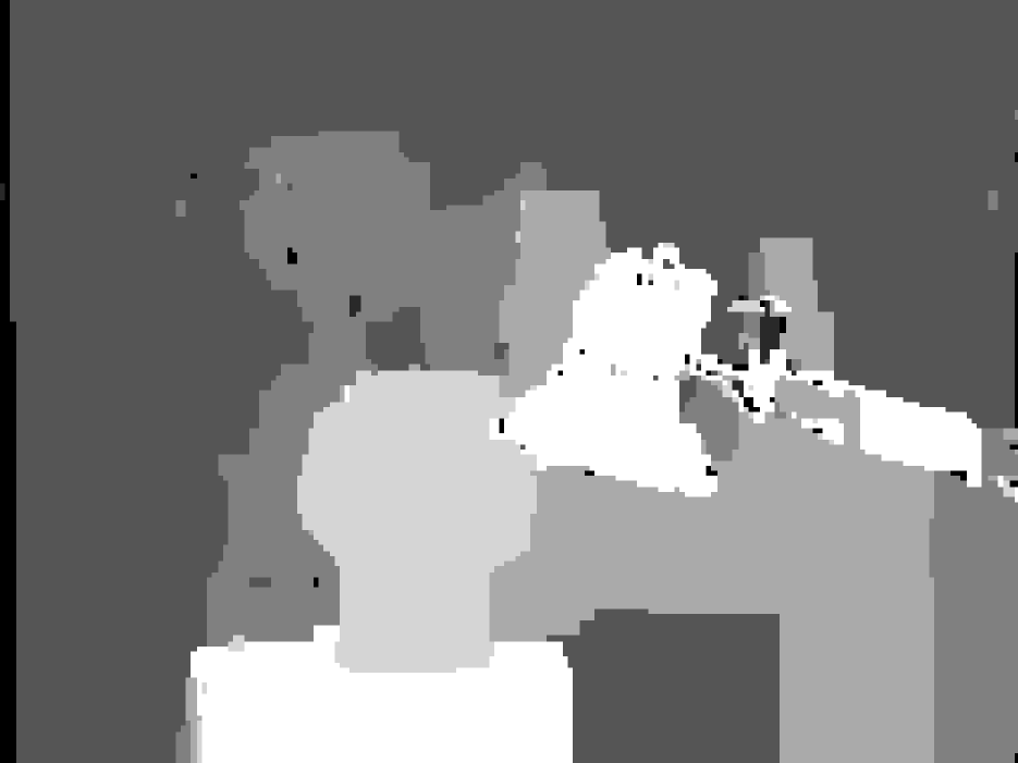
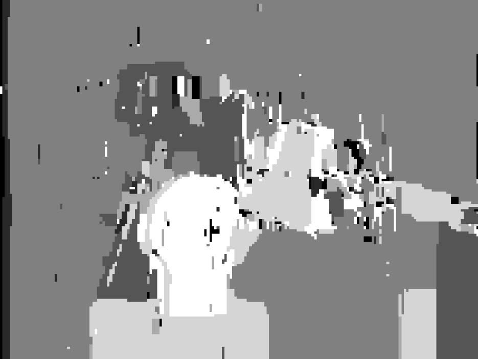
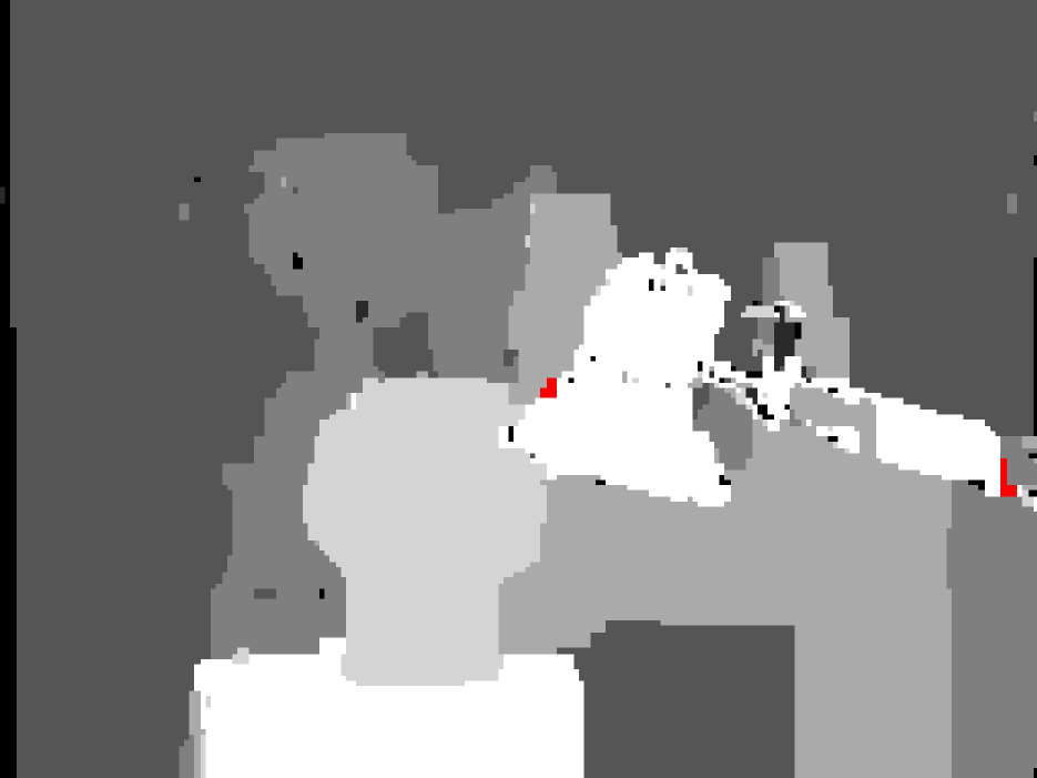
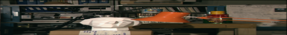
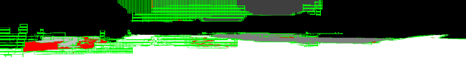
We focus on the MAP inference problem in Markov Random Fields. MAP inference is often used to solve structured prediction problems like stereo vision. The goal of stereo vision is to go from two images—one taken from slightly to the right of the other, like the images seen by your eyes—to an assignment of depths to pixels, which indicates how far each pixel is from the camera. Markov Random Fields give an elegant method for finding the best assignment of states (depths) to variables (pixels), taking into account the structure of the output space. Figure 1 illustrates the need for a better theoretical understanding of MAP inference algorithms. An exact solution to the MAP problem for a real-world stereo vision instance appears in Figure 1(a). Figure 1(b) shows an assignment that, according to the current theory, might be returned by the best approximation algorithms. These two assignments agree on less than 1% of their labels. Finally, Figure 1(c) shows an assignment actually returned by an approximation algorithm—this assignment has over 99% of labels in common with the exact one. This surprising behavior is not limited to stereo vision. Many structured prediction problems have approximate MAP algorithms that perform extremely well in practice despite the exact MAP problems being NP-hard (Koo et al., 2010; Savchynskyy et al., 2013; Kappes et al., 2015; Swoboda et al., 2016).
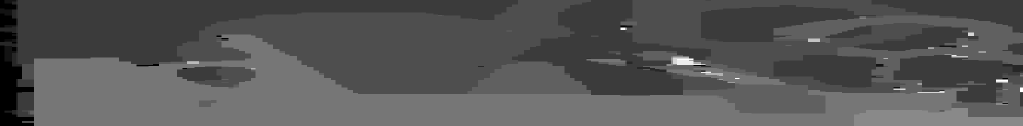
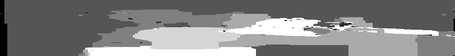
The huge difference between Figures 1(b) and 1(c) indicates that real-world instances must have some structure that makes the MAP problem easy. Indeed, these instances seem to have some stability to multiplicative perturbations. Figure 2 shows MAP solutions to a stereo vision instance and a small perturbation of that instance.111The instances in Figures 1 and 2 have the same input images, but Figure 2 uses higher resolution. These solutions share many common labels, and many portions are exactly the same.

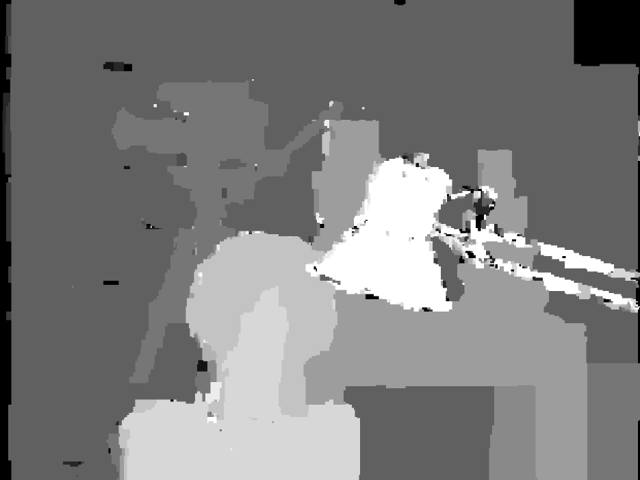
Put simply, in the remainder of this work we attempt to use the structure depicted in Figure 2 to explain why Figure 1(c) is so similar to Figure 1(a).
The approximation algorithm used to produce Figure 1(c) is called the pairwise LP relaxation (Wainwright and Jordan, 2008; Chekuri et al., 2001). This algorithm formulates MAP inference as an integer linear program (ILP) with variables that are constrained to be in . It then relaxes that ILP to a linear program (LP) with constraints , which can be solved efficiently. Unfortunately, the LP solution may not be a valid MAP solution—it may have fractional values —so it might need to be rounded to a MAP solution. However, in practice, the LP solution frequently takes values in , and these values “match” with the exact MAP solution, so very little rounding is needed. For example, the LP solution shown in Figure 1(c) takes binary values that agree with the exact solution on more than 99% of the instance. This property is known as persistency.
Much previous work has gone into understanding the persistency of the LP relaxation, typically stemming from a desire to give partial optimality guarantees for LP solutions and to use persistent solutions as a building block for finding exact MAP solutions. These results use the fact that the pairwise LP is often persistent on large portions of these instances to design fast algorithms for verifying partial optimality and for exact MAP inference (Kovtun, 2003; Savchynskyy et al., 2013; Swoboda et al., 2016; Haller et al., 2018; Shekhovtsov et al., 2018). Contrastingly, our work aims to understand why the LP is persistent so frequently on real-world instances.
Lang et al. (2018) first explored the stability framework of Makarychev et al. (2014) in the context of MAP inference. They showed that under a strong stability condition, the pairwise LP relaxation provably returns an exact MAP solution. Unfortunately, this condition (that the solution does not change at all under perturbations) is rarely, if ever, satisfied in practice. On the other hand, Figure 2 demonstrates that the original and perturbed solutions do have many labels in common, so there could be some stability present at the “sub-instance” level.
In this work, we give an extended stability framework, generalizing the work of Lang et al. (2018) to the setting where only some parts of an instance have stable structure. This naturally connects to work on dual decomposition for MAP inference. We establish a theoretical connection between dual decomposition and stability, which allows us to use stability even when it is only present on parts of an instance, and allows us to combine stability with other reasons for persistency. In particular, we define a new notion called block stability, for which we show the following:
-
•
We prove that approximate solutions returned by the pairwise LP relaxation agree with the exact solution on all the stable blocks of an instance.
-
•
We design an algorithm to find stable blocks on real-world instances.
-
•
We run this algorithm on several examples from low-level computer vision, including stereo vision, where we find that these instances contain large stable blocks.
-
•
We demonstrate that the block framework can be used to incorporate stability with other structural reasons for persistency of the LP relaxation.
Taken together, these results suggest that block stability is a plausible explanation for the empirical success of LP-based algorithms for MAP inference.
2 BACKGROUND
2.1 MAP Inference and Metric Labeling
A Markov Random Field consists of a graph , a discrete set of labels , and potential functions that capture the cost of assignments . The MAP inference task in a Markov Random Field is to find the assignment (or labeling) with the lowest cost:
| (1) |
Here we have decomposed the set of potential functions functions into and , which correspond to nodes and edges in the graph , respectively. A Markov Random Field that can be decomposed in this manner is known as a pairwise MRF; we focus exclusively on pairwise MRFs. In equation (1), the single-node potential functions represent the cost of assigning label to node , and the pairwise potentials represent the cost of simultaneously assigning label to node and label to node .
The MAP inference problem has been extensively studied for special cases of the potential functions . When the pairwise potential functions take the form
the model is called a generalized Potts model. When the weights are nonnegative, as they are throughout this paper, the model is called ferromagnetic or attractive. This formulation has enjoyed a great deal of use in the computer vision community, where it has proven especially useful for modeling low-level problems like stereo vision, segmentation, and denoising (Boykov et al., 2001; Tappen and Freeman, 2003). With this special form of , we can re-write the MAP inference objective as:
| (2) |
Here we have defined as the objective of a feasible labeling . We can then call an instance of MAP inference for a Potts model with node costs and weights .
The minimization problem (2) is also known as Uniform Metric Labeling, and was first defined and studied under that name by Kleinberg and Tardos (2002). Exact minimization of the objective (2) is NP-hard (Kleinberg and Tardos, 2002), but many good approximation algorithms exist. Most notably for our work, Kleinberg and Tardos (2002) give a 2-approximation based on the pairwise LP relaxation (3).222Kleinberg and Tardos (2002) use the so-called “metric LP,” but this is equivalent to (3) for Potts potentials (Archer et al., 2004; Lang et al., 2018), and their rounding algorithm also works for this formulation.
| (3) |
Their algorithm rounds a solution of (3) to a labeling that is guaranteed to satisfy . The decision variables represent the (potentially fractional) assignment of label at vertex . While solutions to (3) might, in general, take fractional values , solutions are often found to be almost entirely binary-valued in practice (Koo et al., 2010; Meshi et al., 2016; Swoboda et al., 2016; Savchynskyy et al., 2013; Kappes et al., 2015), and these values are typically the same ones taken by the exact solution to the original problem. Figure 1(c) demonstrates this phenomenon. In other words, it is often the case in practice that if , then , where and are solutions to (2) and (3), respectively. This property is called persistency (Adams et al., 1998). We say a solution is persistent at if and for some .
This LP approach to MAP inference has proven popular in practice because it is frequently persistent on a large percentage of the vertices in an instance, and because researchers have developed several fast algorithms for solving (3). These algorithms typically work by solving the dual; Tree-reweighted Message Passing (TRW-S) (Kolmogorov, 2006), MPLP (Globerson and Jaakkola, 2008), and subgradient descent (Sontag et al., 2012) are three well-known dual approaches. Additionally, the introduction of fast general-purpose LP solvers like Gurobi (Gurobi Optimization, 2018) has made it possible to directly solve the primal (3) for medium-sized instances.
2.2 Stability
An instance of an optimization problem is stable if its solution doesn’t change when the input is perturbed. To discuss stability formally, one must specify the exact type of perturbations considered. As in Lang et al. (2018), we study multiplicative perturbations of the weights:
Definition 1 (-perturbation, Lang et al. (2018)).
Given a weight function , a weight function is called a -perturbation of if for any ,
With the perturbations defined, we can formally specify the notion of stability:
Definition 2 (-stable, Lang et al. (2018)).
A MAP inference instance with graph , node costs , weights , labels , and integer solution is called -stable if for any -perturbation of , and any labeling , where is the objective with costs and weights .
That is, is the unique solution to the optimization (2) where is replaced by any valid -perturbation of . As and increase, the stability condition becomes increasingly strict. One can show that the LP relaxation (3) is tight (returns an exact solution to (2)) on suitably stable instances:
Theorem 1 (Theorem 1, Lang et al. (2018)).
Let be a solution to the LP relaxation (3) on a (2,1)-stable instance with integer solution . Then .
Many researchers have used stability to understand the real-world performance of approximation algorithms. Bilu and Linial (2010) introduced perturbation stability for the Max Cut problem. Makarychev et al. (2014) improved their result for Max Cut and gave a general framework for applying stability to graph partitioning problems. Lang et al. (2018) extended their results to MAP inference in Potts models. Stability has also been applied to clustering problems in machine learning (Balcan et al., 2009, 2015; Balcan and Liang, 2016; Awasthi et al., 2012; Dutta et al., 2017).
3 BLOCK STABILITY
The current stability definition used in results for the LP relaxation (Definition 2) requires that the MAP solution does not change at all for any -perturbation of the weights . This strong condition is rarely satisfied by practical instances such as those in Figure 1 and Figure 2. However, it may be the case that the instance is -stable when restricted to large blocks of the vertices. We show in Section 5 that this is indeed the case in practice, but for now we precisely define what it means to be block stable, where some parts of the instance may be stable, but others may not. We demonstrate how to connect the ideas of dual decomposition and stability, working up to our main theoretical result in Theorem 2. Appendix A.1 contains proofs of the statements in this section.
We begin our discussion with an informal version of our main theorem:
Informal Theorem (see Theorem 2).
Assume an instance has a block that is -stable and has some additional, additive stability with respect to the node costs for nodes along the boundary of . Then the LP (3) is persistent on .
To reason about different blocks of an instance (and eventually prove persistency of the LP on them), we need a way to decompose the instance into subproblems so that we can examine each one more or less independently. The dual decomposition framework (Sontag et al., 2012; Komodakis et al., 2011) provides a formal method for doing so. The commonly studied Lagrangian dual of (3), which we call the pairwise dual, turns every node into its own subproblem:
| (4) |
This can be derived by introducing Lagrange multipliers on the two consistency constraints for each edge and each :
Many efficient solvers for (4) have been developed, such as MPLP (Globerson and Jaakkola, 2008). But the subproblems in (4) are too small for our purposes. We want to find large portions of an instance with stable structure. Given a set , define to be the set of edges with both endpoints in , and let . We may consider relaxing fewer consistency constraints than (4) does, to form a block dual with blocks and .
| (5) |
subject to the following constraints for :
| (6) |
Here the consistency constraints of (3) are only relaxed for boundary edges that go between and , denoted by . Each subproblem (each minimization over ) is an LP of the same form as (3), but is defined only on the block (either or , in this case). If , the block dual is equivalent to the primal LP (3). We denote the constraint set (6) by . In these subproblems, the node costs are modified by , the sum of the block dual variables coming from the other block. We can thus rewrite each subproblem as an LP of the form:
where
| (7) |
By definition, is equal to on the interior of each block. It only differs from on the boundaries of the blocks. We show in Appendix A.1 how to turn a solution of (4) into a solution of (LABEL:eq:blockdual); this block dual is efficiently solvable. The form of suggests the following definition for a restricted instance:
Definition 3 (Restricted Instance).
Consider an instance of MAP inference, and let . The instance restricted to with modification is given by:
where is as in (7) and is restricted to , and the weights are restricted to .
Given a set , let be a solution to the block dual (LABEL:eq:blockdual). We essentially prove that if the instance restricted to , with modification , is -stable, the LP solution to the original LP (3) (defined on the full, unmodified instance) takes binary values on :
Lemma 1.
Consider the instance . Let be any subset of vertices, and let be any solution to the block dual (LABEL:eq:blockdual). Let be the solution to (3) on this instance. If the restricted instance
is -stable with solution , then .
Here is the exact solution to the restricted instance with node costs modified by . This may or may not be equal to , the overall exact solution restricted to the set . If , Lemma 1 implies that the LP solution is persistent on :
Corollary 1.
Finally, we can reinterpret this result from the lens of stability by defining additive perturbations of the node costs . Let be the boundary of set ; i.e. the set of such that has a neighbor that is not in .
Definition 4 (-bounded cost perturbation).
Given a subset , node costs , and a function
a cost function is an -bounded perturbation of (with respect to ) if the following equation holds for some with for all :
In other words, a perturbation is allowed to differ from by at most for in the boundary of , and must be equal to everywhere else.
Definition 5 (Stable with cost perturbations).
A restricted instance with solution is called -stable if for all -bounded cost perturbations of , the instance is -stable. That is, is the unique solution to all the instances with an -bounded perturbation of and a -perturbation of .
Theorem 2.
Definition 5 and Theorem 2 provide the connection between the dual decomposition framework and stability: by requiring stability to additive perturbations of the node costs along the boundary of a block , where the size of the perturbation is determined by the block dual variables, we can effectively isolate from the rest of the instance and apply stability to the modified subproblem.
In Appendix A.4, we show how to use the dual decomposition techniques from this section to combine stability with other structural reasons for persistency of the LP on the same instance.
4 FINDING STABLE BLOCKS
In this section, we present an algorithm for finding stable blocks in an instance. We begin with a procedure for testing -stability as defined in Definition 2. Lang et al. (2018) prove that it is sufficient to look for labelings that violate stability in the adversarial perturbation
which tries to make the exact solution as bad as possible. With that in mind, we can try to find a labeling such that , subject to the constraint that (here is the objective with costs and weights . The instance is -stable if and only if no such exists. We can write such a procedure as the following optimization problem:
| (8) |
The first five sets of constraints ensure that forms a feasible integer labeling . The objective function captures the normalized Hamming distance between this labeling and the solution ; it is linear in the decision variables because is fixed— if and 0 otherwise. Of course, the “objective constraint” is also linear in . We have only linear and integrality constraints on , so we can solve (8) with a generic ILP solver such as Gurobi (Gurobi Optimization, 2018). This procedure is summarized in Algorithm 1. Put simply, the algorithm tries to find the labeling that is most different from (in Hamming distance) subject to the constraint that . By construction, the instance is stable if and only if the optimal objective value of this ILP is 0. If there is a positive objective value, there is some with but ; this violates stability. The program is always feasible because satisfies all the constraints. Because it solves an ILP, CheckStable is not a polynomial time algorithm, but we were still able to use it on real-world instances of moderate size in Section 5.
We now describe our heuristic algorithm for finding regions of an input instance that are -stable after their boundary costs are perturbed. Corollary 1 implies that we do not need to test for -stability for all -bounded perturbations of node costs—we can simply check with respect to the one given by (7) with . That is, we need only check for -stability in the instance with node costs . This is enough to guarantee persistency.
In each iteration, the algorithm begins with a partition (henceforth “decomposition” or “block decomposition”) of the nodes into disjoint sets . It then finds a block dual solution for each (see Appendix B.1 for details) and computes the restricted instances using the optimal block dual variables to modify the node costs. Next, it uses Algorithm 1 to check whether these modified instances are -stable. Based on the results of CheckStable, we either update the previous decomposition or verify that a block is stable, then repeat.
All that remains are the procedures for initializing the algorithm and updating the decomposition in each iteration given the results of CheckStable. The initial decomposition consists of blocks, with
| (9) |
So blocks consist of the interiors of the label sets of —a vertex belongs to if and all its neighbors have . The boundary vertices— such that there is some with —are added to a special boundary block denoted by . Some blocks may be empty if is not surjective.
In an iteration of the algorithm, for every block, CheckStable returns a labeling that satisfies and might also have . If , the block is stable and we do nothing. Otherwise, we remove the vertices and add them to the boundary block .
Finally, we try to reclaim vertices from the old boundary block. Like all the other blocks, the boundary block gets tested for stability in each iteration. Some of the vertices in this block may have . We call this the remainder set . We run breadth-first-search in to identify connected components of vertices that get the same label from . Each of these components becomes its own new block, and is added to the block decomposition for the next step. This heuristic prevents the boundary block from growing too large and significantly improves our experimental results, since the boundary block is rarely stable. The entire procedure is summarized in Algorithm 2.
5 EXPERIMENTS
We focus in this section on instances where the pairwise LP performs very well. The examples studied here are more extensively examined in Kappes et al. (2015), where they also compare the effectiveness of the LP to other MAP inference algorithms. Most importantly, though, they observe that the pairwise LP takes fractional values only at a very small percentage of the nodes on these instances. This makes them good candidates for a stability analysis.


5.1 Object Segmentation
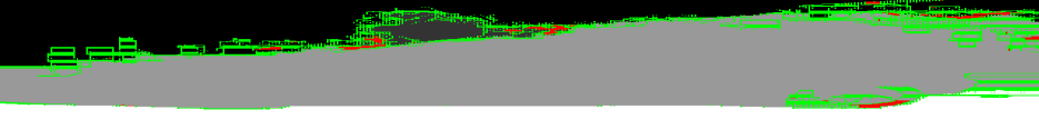
For the object segmentation problem, the goal is to partition the pixels of the input image into a handful of different objects based on the semantic content of the image. The first two rows of figure 3 show some example object segmentation instances. We study a version of the segmentation problem where the number of desired objects is known. We use the model of Alahari et al. (2010); full details about the MRFs used in this experiment can be found in Appendix B. Each instance has 68,160 nodes and either five or eight labels, and we ran Algorithm 2 for iterations to find -stable blocks. The LP (3) is persistent on 100% of the nodes for all three instances we study.
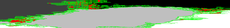
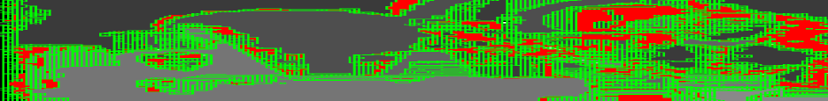
Row 3 of Figure 3 shows the output of Algorithm 2 on each segmentation instance. The red vertices are regions where the algorithm was unable to find a large stable block. The green pixels represent a boundary between blocks, demonstrating the block structure. The largest blocks seem to correspond to objects in the original image (and regions in the MAP solution).
One interesting aspect of these instances is the large number of stable blocks with for the Road instance (Column 2). If the LP is persistent at a node , there is a trivial decomposition in which belongs to its own stable block (see Appendix A.3 for discussion on block size). However, the existence of stable blocks with size is not implied by persistency, so the presence of such blocks means the instances have special structure. The red regions in Figure 3, Row 3 could be replaced by stable blocks of size one. However, Algorithm 2 did not find the trivial decomposition for those regions, as it did for the center of the Road instance. We believe the large number of blocks with for the Road instance could therefore be due to our “reclaiming” strategy in Algorithm 2, which does not try to merge together reclaimed blocks, rather than a lack of stability in that region.
5.2 Stereo Vision
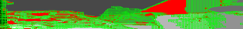
As we discussed in Section 1, the stereo vision problem takes as input two images and of the same scene, where is taken from slightly to the right of . The goal is to output a depth label for each pixel in that represents how far that pixel is from the camera. Depth is inversely proportional to the disparity (how much the pixel moves) of the pixel between the images and . So the goal is to estimate the (discretized) disparity of each pixel. The first two rows of Figure 3 show three example instances and their MAP solutions. We use the MRF formulation of Boykov et al. (2001) and Tappen and Freeman (2003). The exact details of these stereo MRFs can be found in Appendix B. These instances have between 23,472 and 27,684 nodes, and between 8 and 16 labels. The LP (3) is persistent on 98-99% of each instance.
Row 3 of Figure 3 shows the results of Algorithm 2 for the stereo instances. As with object segmentation, we observe that the largest stable blocks tend to coincide with the actual objects in the original image. Compared to segmentation, fewer vertices in these instances seem to belong to large stable blocks. We believe that decreased resolution may play a role in this difference. The computational challenge of scaling Algorithms 1 and 2 to the stereo model forced us to use downsampled (0.5x or smaller) images to form the stereo MRFs. Brief experiments with higher resolution suggest that improving the scalability of Algorithm 2 is an interesting avenue for improving these results.
6 DISCUSSION
The block stability framework we presented helps to understand the tightness and persistency of the pairwise LP relaxation for MAP inference. Our experiments demonstrate that large blocks of common computer vision instances are stable. While our experimental results are for the Potts model, our extension from -stability to block stability uses no special properties of the Potts model and is completely general. If a -stability result similar to Theorem 1 is given for other pairwise potentials, the techniques used here immediately give the analogous version of Theorem 2. Our results thus give a connection between dual decomposition and stability.
The method used to prove the results in Section 3 can even extend beyond stability. We only need stability to apply Theorem 1 to a modified block. Instead of stability, we could plug in any result that guarantees the pairwise LP on that block has a unique integer solution. Appendix A gives an example of incorporating stability with tree structure on the same instance. Combining different structures to fully explain persistency on real-world instances will require new algorithmic insight.
The stability of these instances suggests that designing new inference algorithms that directly take advantage of stable structure is an exciting direction for future research. The models examined in our experiments use mostly hand-set potentials. In settings where the potentials are learned from training data, is it possible to encourage stability of the learned models?
Acknowledgments
The authors would like to thank Fredrik D. Johansson for his insight during many helpful discussions. This work was supported by NSF AitF awards CCF-1637585 and CCF-1723344. AV is also supported by NSF Grant No. CCF-1652491.
References
References
- Adams et al. (1998) Warren P Adams, Julie Bowers Lassiter, and Hanif D Sherali. Persistency in 0-1 polynomial programming. Mathematics of operations research, 23(2):359–389, 1998.
- Alahari et al. (2010) Karteek Alahari, Pushmeet Kohli, and Philip HS Torr. Dynamic hybrid algorithms for map inference in discrete mrfs. IEEE Transactions on Pattern Analysis and Machine Intelligence, 32(10):1846–1857, 2010.
- Archer et al. (2004) Aaron Archer, Jittat Fakcharoenphol, Chris Harrelson, Robert Krauthgamer, Kunal Talwar, and Éva Tardos. Approximate classification via earthmover metrics. In Proceedings of the Fifteenth Annual ACM-SIAM Symposium on Discrete Algorithms, SODA ’04, pages 1079–1087, Philadelphia, PA, USA, 2004. Society for Industrial and Applied Mathematics. ISBN 0-89871-558-X.
- Awasthi et al. (2012) Pranjal Awasthi, Avrim Blum, and Or Sheffet. Center-based clustering under perturbation stability. Information Processing Letters, 112(1):49–54, 2012.
- Balcan and Liang (2016) Maria-Florina Balcan and Yingyu Liang. Clustering under perturbation resilience. 2016.
- Balcan et al. (2009) Maria-Florina Balcan, Avrim Blum, and Anupam Gupta. Approximate clustering without the approximation. In Proceedings of the twentieth Annual ACM-SIAM Symposium on Discrete Algorithms, SODA ’09, pages 1068–1077, 2009.
- Balcan et al. (2015) Maria-Florina Balcan, Nika Haghtalab, and Colin White. Symmetric and asymmetric -center clustering under stability. arXiv preprint arXiv:1505.03924, 2015.
- Bilu and Linial (2010) Yonatan Bilu and Nathan Linial. Are stable instances easy? In Innovations in Computer Science, pages 332–341, 2010.
- Birchfield and Tomasi (1998) Stan Birchfield and Carlo Tomasi. A pixel dissimilarity measure that is insensitive to image sampling. IEEE Transactions on Pattern Analysis and Machine Intelligence, 20(4):401–406, 1998.
- Boykov et al. (2001) Y. Boykov, O. Veksler, and R. Zabih. Fast approximate energy minimization via graph cuts. IEEE Transactions on Pattern Analysis and Machine Intelligence, 23(11):1222–1239, Nov 2001. ISSN 0162-8828.
- Chekuri et al. (2001) Chandra Chekuri, Sanjeev Khanna, Joseph (Seffi) Naor, and Leonid Zosin. Approximation algorithms for the metric labeling problem via a new linear programming formulation. In Proceedings of the Twelfth Annual ACM-SIAM Symposium on Discrete Algorithms, SODA ’01, pages 109–118, Philadelphia, PA, USA, 2001. Society for Industrial and Applied Mathematics. ISBN 0-89871-490-7.
- Dutta et al. (2017) Abhratanu Dutta, Aravindan Vijayaraghavan, and Alex Wang. Clustering stable instances of euclidean -means. In Advances in Neural Information Processing Systems (to appear), 2017.
- Globerson and Jaakkola (2008) Amir Globerson and Tommi S Jaakkola. Fixing max-product: Convergent message passing algorithms for map lp-relaxations. In Advances in neural information processing systems, pages 553–560, 2008.
- Gurobi Optimization (2018) LLC Gurobi Optimization. Gurobi optimizer reference manual, 2018. URL http://www.gurobi.com.
- Haller et al. (2018) Stefan Haller, Paul Swoboda, and Bogdan Savchynskyy. Exact map-inference by confining combinatorial search with lp relaxation. In Proceedings of the 32st AAAI Conference on Artificial Intelligence, 2018.
- Kappes et al. (2015) Jörg H Kappes, Bjoern Andres, Fred A Hamprecht, Christoph Schnörr, Sebastian Nowozin, Dhruv Batra, Sungwoong Kim, Bernhard X Kausler, Thorben Kröger, Jan Lellmann, et al. A comparative study of modern inference techniques for structured discrete energy minimization problems. International Journal of Computer Vision, 115(2):155–184, 2015.
- Kleinberg and Tardos (2002) Jon Kleinberg and Éva Tardos. Approximation algorithms for classification problems with pairwise relationships: Metric labeling and markov random fields. J. ACM, 49(5):616–639, September 2002. ISSN 0004-5411.
- Kolmogorov (2006) Vladimir Kolmogorov. Convergent tree-reweighted message passing for energy minimization. IEEE transactions on pattern analysis and machine intelligence, 28(10):1568–1583, 2006.
- Komodakis et al. (2011) Nikos Komodakis, Nikos Paragios, and Georgios Tziritas. Mrf energy minimization and beyond via dual decomposition. IEEE transactions on pattern analysis and machine intelligence, 33(3):531–552, 2011.
- Koo et al. (2010) Terry Koo, Alexander M. Rush, Michael Collins, Tommi Jaakkola, and David Sontag. Dual decomposition for parsing with non-projective head automata. In Proceedings of the 2010 Conference on Empirical Methods in Natural Language Processing (EMNLP), pages 1288–1298, 2010.
- Kovtun (2003) Ivan Kovtun. Partial optimal labeling search for a np-hard subclass of (max,+) problems. In Joint Pattern Recognition Symposium, pages 402–409. Springer, 2003.
- Lang et al. (2018) Hunter Lang, David Sontag, and Aravindan Vijayaraghavan. Optimality of approximate inference algorithms on stable instances. In Proceedings of the Twenty-First International Conference on Artificial Intelligence and Statistics. PMLR, 2018.
- Makarychev et al. (2014) Konstantin Makarychev, Yury Makarychev, and Aravindan Vijayaraghavan. Bilu-linial stable instances of max cut and minimum multiway cut. In Proceedings of the twenty-fifth annual ACM-SIAM symposium on Discrete algorithms, pages 890–906. Society for Industrial and Applied Mathematics, 2014.
- Meshi et al. (2016) Ofer Meshi, Mehrdad Mahdavi, Adrian Weller, and David Sontag. Train and test tightness of lp relaxations in structured prediction. In Maria Florina Balcan and Kilian Q. Weinberger, editors, Proceedings of The 33rd International Conference on Machine Learning, volume 48 of Proceedings of Machine Learning Research, pages 1776–1785, New York, New York, USA, 20–22 Jun 2016. PMLR.
- Savchynskyy et al. (2013) Bogdan Savchynskyy, Jörg Hendrik Kappes, Paul Swoboda, and Christoph Schnörr. Global map-optimality by shrinking the combinatorial search area with convex relaxation. In Advances in Neural Information Processing Systems, pages 1950–1958, 2013.
- Shekhovtsov et al. (2018) Alexander Shekhovtsov, Paul Swoboda, and Bogdan Savchynskyy. Maximum persistency via iterative relaxed inference with graphical models. IEEE Transactions on Pattern Analysis and Machine Intelligence, 40(7), 2018.
- Shotton et al. (2006) Jamie Shotton, John Winn, Carsten Rother, and Antonio Criminisi. Textonboost: Joint appearance, shape and context modeling for multi-class object recognition and segmentation. In European conference on computer vision, pages 1–15. Springer, 2006.
- Sontag et al. (2012) David Sontag, Amir Globerson, and Tommi Jaakkola. Introduction to dual decomposition for inference. In Suvrit Sra, Sebastian Nowozin, and Stephen J. Wright, editors, Optimization for Machine Learning, pages 219–254. MIT Press, 2012.
- Swoboda et al. (2016) Paul Swoboda, Alexander Shekhovtsov, Jorg Hendrik Kappes, Christoph Schnorr, and Bogdan Savchynskyy. Partial optimality by pruning for map-inference with general graphical models. IEEE Transactions on Pattern Analysis and Machine Intelligence, 38(7):1370–1382, 2016.
- Tappen and Freeman (2003) Marshall F Tappen and William T Freeman. Comparison of graph cuts with belief propagation for stereo, using identical mrf parameters. In null, page 900. IEEE, 2003.
- Wainwright and Jordan (2008) Martin J Wainwright and Michael I Jordan. Graphical models, exponential families, and variational inference. Foundations and Trends® in Machine Learning, 1(1–2):1–305, 2008.
Appendix A Theory Details
In this appendix, we give a complete exposition and proof of Lemma 1 and use it to prove Theorem 2 from Section 3. We also discuss a subtlety regarding the size of stable blocks, and show that adding perturbations to the node costs seems necessary to prove Lemma 1.
A.1 Proofs of Lemma 1 and Theorem 2
We now more formally develop the connection between the block dual (LABEL:eq:blockdual) and block stability. To begin, the pairwise dual of the LP (3) is given by:
| (10) |
This can be derived by introducing Lagrange multipliers on the two consistency constraints for each edge and each :
A dual point is said to be locally decodable at a node if the cost terms
have a unique minimizing label . This dual has the following useful properties for studying persistency of the LP (3):
Property 1 (Strong Duality).
Property 2 (Complementary Slackness, Sontag et al. (2012) Theorem 1.2).
If is a primal solution to the pairwise LP (3) and there exists a dual solution that is locally decodable at node to label , then . That is, if the dual solution is locally decodable at node , the primal solution is not fractional at node .
Property 3 (Strict Complementary Slackness, Sontag et al. (2012) Theorem 1.3).
In particular, Property 2 says that to prove the primal LP is persistent at a vertex , we need only exhibit a dual solution to (4) that is locally decodable at to , where is an integer MAP solution. Properties 1 and 3 will be useful for proving results about a different Lagrangian dual that relaxes fewer constraints, which we study now.
Given a partition (henceforth a “block decomposition”), we may consider relaxing fewer consistency constraints than (4) does, to form a block dual.
| (11) |
subject to the following constraints for all :
| (12) |
This is simply a more general version of the dual (LABEL:eq:blockdual), written for an arbitrary partition . Here the consistency constraints are only relaxed for edges in (boundary edges, which go from one block to another). The dual subproblems in the first term of (LABEL:eq:blockdual_gen) are LPs on each block, where the node costs of boundary vertices are modified by the block dual variables . For any , we can define the reparametrized costs as
so the block dual objective can also be written as
When there is only one block, equal to , the block dual is equivalent to the primal LP (3). When every vertex is in its own block, the block dual is equivalent to the pairwise dual (4).
The following propositions allow us to convert between solutions of the pairwise dual (4) and the generalized block dual (LABEL:eq:blockdual_gen).
Proposition 1.
Let be a solution to (4). Let be the restriction of to the domain of ; that is, is defined only for pairs , such that or :
Then is a a solution to (LABEL:eq:blockdual_gen).
This proposition gives a simple method for converting a solution to pairwise dual to a solution to the block dual : simply restrict it to the domain of . As we explain in Appendix B, this allows us to avoid ever solving the block dual directly; we simply solve the pairwise dual once, and can then easily form a block dual solution for any set of blocks.
Proof.
It is clear that defined in this way is dual-feasible (there are no constraints on the ’s). We show that . Let be a primal LP solution. Because for any dual-feasible (this is easy to verify), and (Property 1), this implies . must then be a solution for the block dual . Note that this proof also implies strong duality for the block dual.
To see that , one could observe intuitively that is strictly more constrained than unless every vertex is its own block; since the subproblems are all minimization problems, the optimal objective of will be higher. More formally, consider two adjacent nodes and in the pairwise dual . The terms corresponding to in in can be written as:
where is the set of vertices adjacent to . The terms written here do not appear in (4) because the minimum choice at a single vertex can clearly be chosen by for a label that minimizes the reparametrized potential, but we have left them in for convenience (under the constraint that ). By the convexity of , the value of the objective above is at most
Adding a new constraint to this minimization problem can only increase the objective value, so the value of the objective above is at most the value of:
subject to the constraints for all and for all . Now the vertices and have been combined into a block. One can continue in this way, enforcing consistency constraints within blocks, until arriving at:
where the minimizations over on the right-hand-side are subject to the constraints (12). The left-hand side is . The expression on the right hand side is precisely the objective of , since we defined as the restriction of to edges in . This completes the proof. ∎
Corollary 2 (Strong duality for block dual).
If is a primal solution and is a solution to the block dual, .
So we are able to easily convert between a pairwise dual solution and a solution to the block dual. This will prove convenient for two reasons: there are many efficient pairwise dual solvers, so we can quickly find . Additionally, we can solve the pairwise dual once and convert the solution into solutions to the block dual for any block decomposition without having to recompute a solution. As we mentioned above, this will allow us to quickly test different block decompositions.
The following proposition allows us to convert a solution to the block dual to a pairwise dual solution.
Proposition 2.
Let be a solution to the block dual (LABEL:eq:blockdual_gen). Recall that each subproblem of the block dual is an LP of the same form as (3). So we can consider the pairwise dual defined on this subproblem. For block , let be a solution to the pairwise dual defined on that block’s (reparametrized) subproblem. That is,
Then the point defined as
is a solution to (4).
Given a solution to the block dual, we use Proposition 2 to extend it to a solution to the pairwise dual defined on the full instance; combining with pairwise dual solutions on the subproblems induced by and the block decomposition gives an optimal .
Proof.
With this proposition, we are finally ready to prove Lemma 1.
Proof of Lemma 1.
We are given a Potts instance . Let be a solution to (LABEL:eq:blockdual_gen) with and . We know the sub-instance
is -stable. Let be the exact solution to the instance . If is the exact solution for , may or may not be the same as . For this Lemma, they need not be equal, and we just work with . Because of the -stability, Theorem 1 implies that is the unique solution to the following LP:
This LP is simply the pairwise LP (3) defined on . Strict complementary slackness (Property 3) implies that the pairwise dual problem defined on has a solution that is locally decodable to . That is, there is some with
and for all ,
In other words, is the unique minimizer of the modified node costs at . By Proposition 1, we can extend and to a solution to the pairwise dual (4) defined on . This extended solution is locally decodable to on by construction. If is a solution to the primal LP (3) defined on , complementary slackness (Property 2) implies that for all . That is, the LP solution is equal to on . ∎
Nothing special was used about the block decomposition , and indeed Lemma 1 also holds for an arbitrary decomposition ; if the instance restricted to a block is -stable after its node costs are perturbed by a solution to the block dual (LABEL:eq:blockdual_gen), the primal LP is equal on to the exact solution of that restricted instance.
It is clear from Lemma 1 that if the solutions to the restricted instances are equal to (the exact solution to the full problem, restricted to ), the primal LP is persistent on (this is formalized in Corollary 1). This is why Theorem 2 requires that the restricted instance is stable with solution .
Proof of Theorem 2.
A.2 Do we need dual variables?
A simpler definition for block stability would be that a block is stable if the instance
is -stable. Unfortunately, this is not enough to guarantee persistency. Consider the counterexample in Figure 4.
| Node | Costs | ||
|---|---|---|---|
| u | 0 | ||
| v | 0 | ||
| w | 0 | ||
The optimal integer solution labels and with label 2, and with label 1, for a total objective of 2. The optimal LP solutions assigns weight 0.5 to each label with non-infinite cost, for a total objective of for any . Define the block decomposition , , . Note that each block has a unique optimal solution given by the minimum-cost label, and that these labels match the ones assigned in the combined optimal solution . Every vertex in this instance therefore belongs to an -stable block, according to the simpler definition, but the LP is not persistent anywhere. It is relatively straightforward to check that this instance does not satisfy Definition 5 or the conditions of Lemma 1.
A.3 Stable block size
Assume the pairwise dual solution is locally decodable on vertex to the label , where is the exact solution. Then the reparametrized node costs have a unique minimizing label . Now consider solving the block dual (LABEL:eq:blockdual_gen) when is a block with just one vertex, . Around block , is a solution to the block dual (see Proposition 1). But this means that is a -stable block with the modified node costs (there are no edges to perturb, and the node costs have a unique minimizer). In this way, it is trivial to give a stable block decomposition any time the LP (3) is persistent on a node —simply add to its own block. However, it is not possible a priori to find stable blocks of size greater than one, and we show in Section 5 that many such blocks exist in practice. These practical instances therefore exhibit structure that is more special than persistency: large stable blocks are not to be expected from persistency alone, and their existence implies persistency.
A.4 Combining stability with other structure
| Node | Costs | ||
|---|---|---|---|
| 1 | 2 | 3 | |
| u | 0 | 0 | 2 |
| v | 0 | ||
| w | 0 | 0 | 2 |
| x | 2 | 0 | 2 |
| y | 2 | 0 | 2 |
| z | 0 | 1 | 1 |
| Node | Opt. Label |
|---|---|
| u | 1 |
| v | 1 |
| w | 1 |
| x | 2 |
| y | 2 |
| z | 2 |
Consider the instance in Figure 5. The tables in Figure 6 give the original node costs and the exact solution for this instance. The objective of is . The pairwise LP (3) is persistent on this instance. How can we explain that? The instance is not -stable: when the weight between and is multiplied by , the optimal label for switches from 2 to 1. However, if we take to be very small, the blocks and seem loosely coupled, and the strong node costs and connections in suggest it might have some stable structure. Unfortunately, the block is not stable for the same reason that the overall instance is not stable. However, this block is a tree!
It is fairly straightforward to verify that given by
is a solution to the block dual with blocks . Indeed, Figure 7 shows the node costs updated by this solution. If we solve the LP on each modified block, ignoring the edges between and , we get an objective of for and an objective of 1 for . Because this matches the objective of the original exact solution , we know in this case that must be optimal for the block dual.
| Node | Costs | ||
|---|---|---|---|
| 1 | 2 | 3 | |
| u | 0 | 1 | |
| v | 0 | ||
| w | 0 | 1 | |
| x | 2 | 0 | 2 |
| y | 2 | 0 | 2 |
| z | 0 | 1 | 1 |
It can then be shown that the modified block
is -stable: when all the weights of edges in become 1 instead of 2, the solution is still to label and with label 1 for sufficiently small and . Similarly, the block
is a tree with a unique integer solution; because the pairwise LP relaxation is tight on trees (Wainwright and Jordan, 2008), this implies by Property 3 that there is a pairwise dual solution to this restricted instance that is locally decodable. Put together, these two results explain the persistency of the pairwise LP relaxation on the full instance by applying different structure at the sub-instance level.
Appendix B Experimental Details
In this appendix, we provide more details and additional discussion regarding the algorithms and experiments in Sections 4 and 5.
B.1 Explaining Algorithm 2
We briefly give more details on the steps of Algorithm 2. One key point is that we can efficiently compute block dual solutions with very little extra computation per outer iteration of the algorithm. We effectively only need to solve a dual problem once; we can then easily generate block dual solutions for any block decomposition for all subsequent iterations. In practice, we simply find a pairwise dual solution using the MPLP algorithm (Globerson and Jaakkola, 2008), then use Proposition 1 to convert it to a solution of the generalized block dual (LABEL:eq:blockdual_gen) for a given decomposition.
Additionally, we can avoid the expensive component of the inner loop of the algorithm (solving CheckStable for each block ). To parallelize CheckStable without any additional work, we modify the node costs of each block using the solution to the generalized block dual, then remove all the edges in . We can then solve the ILP (8) used in CheckStable with one “objective constraint” for each block. The objective function of (8) decomposes across blocks once is removed. This approach avoids the overhead of explicitly forming and solving the ILP (8) for each block, which is especially helpful as the number of blocks grows large. These optimizations are summarized in Algorithm 3.
B.2 Object Segmentation
Setup: Markov Random Field
We use the formulation of Shotton et al. (2006); Alahari et al. (2010). The graph is a grid with one vertex for each pixel in the original image; the edges connect adjacent pixels. In this model, the node costs are set based on the location of the pixel in the image, the color values at that pixel, and the local shape and texture of the image. The edge weights are set as:
Here , are learned parameters, and is the vector of RGB values for pixel in the image. Shotton et al. (2006) learn the node and edge parameters using a boosting method.333We use pre-built object segmentation models from the OpenGM Benchmark that are based on the models of (Alahari et al., 2010): http://hciweb2.iwr.uni-heidelberg.de/opengm/index.php?l0=benchmark This setup yields an instance of a Potts model (Uniform Metric Labeling), so we can proceed with our algorithms. Many vertices of the object segmentation instances appear to belong to large stable blocks. Unlike with stereo vision, we were able to use the full instances in our experiments, which, as we observed in Section 5, could contribute to the quality of our results for segmentation. Each instance has 68,160 nodes and either five or eight labels. The LP is persistent on 100% of the nodes for all three instances.
B.3 Stereo Vision
Setup: Markov Random Field
To begin, we let the graph be a grid graph where each node corresponds to a pixel in . We then need to set the costs for each , , and the weights for each edge in the grid. This is where the domain knowledge enters the problem. For a pixel , we set its cost for disparity as:
| (13) |
Here and are the pixel intensity functions for the images and , respectively, and the notation shifts a pixel location by pixels to the left. That is, if corresponds to location , corresponds to location . If the difference (13) is high, then it is unlikely that pixel actually moved pixels between the two images. On the other hand, if this difference is low, disparity is a plausible choice for pixel . In our experiments, we use a small correction to (13) that accounts for image sampling (Birchfield and Tomasi, 1998); this correction is also used by Boykov et al. (2001) and Tappen and Freeman (2003).
We can set the weights using a similar intuition. If and are neighboring pixels and is similar to , then and probably belong to the same object, so they should probably get the same disparity label. In this case, the weight between them should be high. On the other hand, if is very different from , and may not belong to the same object, so they should have a low weight—they may move different amounts between the two images. To this end, we set
In our experiments, we follow Tappen and Freeman (2003) and set , , . This setup gives us a Potts model instance .