Parallelism in Randomized Incremental Algorithms

Abstract

In this paper we show that many sequential randomized incremental algorithms are in fact parallel. We consider algorithms for several problems including Delaunay triangulation, linear programming, closest pair, smallest enclosing disk, least-element lists, and strongly connected components.

We analyze the dependences between iterations in an algorithm, and show that the dependence structure is shallow with high probability, or that by violating some dependences the structure is shallow and the work is not increased significantly. We identify three types of algorithms based on their dependences and present a framework for analyzing each type. Using the framework gives work-efficient polylogarithmic-depth parallel algorithms for most of the problems that we study.

This paper shows the first incremental Delaunay triangulation algorithm with optimal work and polylogarithmic depth, which is an open problem for over 30 years. This result is important since most implementations of parallel Delaunay triangulation use the incremental approach. Our results also improve bounds on strongly connected components and least-elements lists, and significantly simplify parallel algorithms for several problems.

1 Introduction

The randomized incremental approach has been a very useful paradigm for generating simple and efficient algorithms for a variety of problems. There have been many dozens of papers on the topic (e.g., see the surveys [63, 54]). Much of the early work was in the context of computational geometry, but the approach has also been applied to graph algorithms [20, 24]. The main idea is to insert elements one-by-one in random order while maintaining a desired structure. The random order ensures that the insertions are somehow spread out, and worst-case behaviors are unlikely.

The incremental process appears sequential since it is iterative, but in practice incremental algorithms are widely used in parallel implementations by allowing some iterations to start in parallel and using some form of locking to avoid conflicts. Many parallel implementations for Delaunay triangulation and convex hull, for example, are based on the randomized incremental approach [17, 29, 18, 52, 5, 37, 15, 56, 65]. In theory, however, there are still no known bounds for parallel Delaunay triangulation using the incremental approach, nor for many other problems.

In this paper we show that the incremental approach for Delaunay triangulation, and many other problems, is indeed parallel and leads to work-efficient polylogarithmic-depth (time) algorithms for the problems. The results are based on analyzing the dependence graph (more accurately the distribution of dependence graphs over the random order). This technique has recently been used to analyze the parallelism available in a variety of sequential algorithms, including the simple greedy algorithm for maximal independent set [7], the Knuth shuffle for random permutation [66], greedy graph coloring [45], and correlation clustering [55]. The advantage of this method is that one can use standard sequential algorithms with modest change to make them parallel, often leading to very simple parallel solutions. It has also been shown experimentally that the incremental approach leads to practical parallel algorithms [6], and to deterministic parallelism [12, 6].

Problem	Work	Depth	Type
Comparison sorting (Section 3)	$O(n\log n)$	$O(\log n)$	1
Delaunay triangulation, $d$ dims. (Section 4)	$O(n\log n+n^{\lceil d/2\rceil})\dagger$	$O(d\log n\log^{*}n)$	1
2D linear programming (Section 5.1)	$O(n)\dagger$	$O(\log n)$	2
2D closest pair (Section 5.2)	$O(n)\dagger$	$O(\log n\log^{*}n)$	2
Smallest enclosing disk (Section 5.3)	$O(n)\dagger$	$O(\log^{2}n)$	2
Least-element lists (Section 6.1)	$O(W_{{\mbox{\scriptsize\emph{SP}}}}(n,m)\log n)\dagger$	$O(D_{{\mbox{\scriptsize\emph{SP}}}}(n,m)\log n)$	3
Strongly connected components (Section 6.2)	$O(W_{{\mbox{\scriptsize\emph{R}}}}(n,m)\log n)\dagger$	$O(D_{{\mbox{\scriptsize\emph{R}}}}(n,m)\log n)$	3

Table 1: Work and depth bounds for our parallel randomized incremental algorithms. $W_{{\mbox{\scriptsize\emph{SP}}}}(n,m)$ and $D_{{\mbox{\scriptsize\emph{SP}}}}(n,m)$ denote the work and depth, respectively, of a single-source shortest paths algorithm. $W_{{\mbox{\scriptsize\emph{R}}}}(n,m)$ and $D_{{\mbox{\scriptsize\emph{R}}}}(n,m)$ denote the work and depth, respectively, of performing a reachability query. Bounds marked with a $\dagger$ are expected bounds, and the rest are high probability bounds. All bounds are for the arbitrary CRCW PRAM, except for comparison sorting that requires the priority CRCW PRAM. In all cases the work is the same as the sequential incremental algorithm, since the algorithms are effectively equivalent beyond either reordering (Type 1 or 2) or some redundancy (Type 3).

The contributions of the paper can be summarized as follows.

1. We describe a framework for analyzing parallelism in randomized incremental algorithms. We consider three types of dependences (Type 1, 2, and 3), and give general bounds on the depth of algorithms with for each type (Section 2).

2. We show that randomly ordered insertion into a binary search tree is inherently parallel, leading to an almost trivial comparison sorting algorithm taking $O(\log n)$ depth and $O(n\log n)$ work (i.e., $n$ processors), both with high probability on the priority-write CRCW PRAM (Section 3). Surprisingly, we know of no previous description and analysis of this parallel algorithm.

3. We show that an offline variant of Boissonnat and Teillaud’s [13] randomized incremental algorithm for Delaunay triangulation in $d$ dimensions has dependence depth $O(d\log n)$ with high probability (Section 4). We then describe a way to parallelize the algorithm, which leads to a parallel version with $O(d\log n\log\log n)$ depth with high probability, and $O(n\log n+n^{\lceil d/2\rceil})$ work in expectation, on the CRCW PRAM. This is the first incremental construction of Delaunay triangulation with optimal work and polylogarithmic depth. This problem has been open for 30 years, and is important since most implementations of parallel Delaunay triangulation use the incremental approach, but none of them have polylogarithmic depth bounds. Surprisingly, our algorithm is very simple.

4. We show that classic sequential randomized incremental algorithms for constant-dimensional linear programming, closest pair, and smallest enclosing disk have shallow dependence depth (Section 5). This leads to very simple linear-work and polylogarithmic-depth randomized parallel algorithms for all three problems.

5. We show that by relaxing dependences (i.e., allowing some to be violated), two random incremental graph algorithms have (reasonably) shallow dependence depth. The relaxation increases the work, but only by a constant factor in expectation. We apply the approach to generate efficient parallel versions of Cohen’s algorithm [20] for least-element lists (Section 6.1) and Coppersmith et al.’s algorithm [24] for strongly connected components (SCC, Section 6.2). In both cases we improve on the previous best bounds for the problems. Least-element lists have applications to tree embeddings on graph metrics [34, 10], and estimating neighborhood sizes in graphs [21]. Coppersmith et al.’s SCC algorithm [24] is widely used in practice [46, 4, 67, 70]. In this paper, we analyze the parallelism of this algorithm, which had been a long-standing open question. This algorithm was later implemented and shown experimentally to be practical by Dhulipala et al. [28].

Other than the graph algorithms, which call subroutines that are known to be hard to efficiently parallelize (reachability and shortest paths), all of our solutions are work-efficient and run in polylogarithmic depth (time). The bounds for all of our parallel randomized incremental algorithms can be found in Table 1.

Preliminaries

We analyze parallel algorithms in the work-depth paradigm [47]. An algorithm proceeds in a sequence of $D$ (depth) rounds, with round $i$ doing $w_{i}$ work in parallel. The total work is therefore $W=\sum_{i=1}^{D}w_{i}$. We account for the cost of allocating processors and compaction in our depth. Therefore the bounds on a PRAM with $P$ processors is $O(W/P+D)$ time [14]. We use the concurrent-read and concurrent-writes (CRCW) PRAM model. By default, we assume the arbitrary-write CRCW model, but when stated use the priority-write model. We say $O(f(n))$ with high probability (whp) to indicate $O(kf(n))$ with probability at least $1-1/n^{k}$.

2 Iteration Dependences

An iterative algorithm is an algorithm that runs in a sequence of iterations (steps) in order. When applied to a particular input, we refer to the computation as an iterative computation. Iteration $j$ is said to depend on iteration $i<j$ if the computation of iteration $j$ is affected by the computation of iteration $i$. The particular dependences, or even the number of iterations, can be a function of the input, and can be modeled as a directed acyclic graph (DAG)—the iterations ($I={1,\ldots,n}$) are vertices and dependences between them are arcs (directed edges).

Definition 1 (Iteration Dependence Graph [66]).

An iteration dependence graph for an iterative computation is a (directed acyclic) graph $G(I,E)$ such that if every iteration $i\in I$ runs after all predecessor iterations in $G$ have completed, then every iteration will do the same computation as in the sequential order.

We are interested in the depth (longest directed path) of iteration dependence graph since shallow dependence graphs imply high parallelism—at least if the dependences can be determined online, and depth of each iteration can be appropriately bounded. We refer to the depth of the DAG as the iteration dependence depth, and denote it as $D(G)$.

In general there can be sub-iterations nested within each iteration of an algorithm. In this case we can consider the dependences between these sub-iterations instead of the top-level iterations (i.e., a dependence from the sub-iteration in one iteration to the sub-iteration in either the same or different iteration). The iteration dependence graph is defined analogously—dependence edges go between the sub-iterations, possibly in different top-level iterations. In this paper, we only consider one such algorithm, Delaunay triangulation, where the main iterations are over the points, and the sub-iterations are for each triangle created by adding the point.

An incremental algorithm takes a sequence of elements (or objects) $E$, and iteratively inserts then one at a time while maintaining some property over the elements. A randomized incremental algorithm is an incremental algorithm in which the elements are added in a uniformly random order—each permutation is equally likely. In this paper, we are interested in deriving probability bounds over the iteration dependence depth. We consider three types of randomized incremental algorithms, which we refer to as Type 1, 2, and 3, for lack of better names.

2.1 Type 1 Algorithms

In these algorithms we show the probability bounds on iteration dependence depth by considering all possible paths of dependences. By bounding the probability of each path, and bounding the number of possible paths, the union bound can be used to bound the probability that any path is long. We use backwards analysis [63] to analyze the length and number of paths.

We say that an incremental algorithm has $k$-bounded dependences if for any input $E$ and element $e\in E$ inserted last, $e$ directly depends on at most $k$ other elements—i.e., once those up to $k$ other elements are inserted, it is safe to insert $e$. For example, consider sorting by inserting into a binary search tree based on a random order. For any key $v$ inserted last, once the previous and next keys in sorted order, $v_{p}$ and $v_{n}$, have been inserted, we can immediate insert $v$. In particular the key $v$ will either be the right child of $v_{p}$ or the left child of $v_{n}$ depending on which of the two was inserted later. More subtly, the search path for $v$ will also be the same once $v_{p}$ and $v_{n}$ are both inserted (more discussion in Section 3). Inserting into a BST therefore has $2$-bounded dependences.

If the iterations in an incremental algorithm are nested, then we consider the pairs of an element along with each of its sub-iterations. We say that an incremental algorithm has $k$-bounded nested dependences if for any input $E$, any element $e\in E$ inserted last, and any sub-iteration $s$ for $e$, $(e,s)$ directly depends on at most $k$ possible previous element–sub-iteration pairs. We say “possible” here since the sub-iterations might differ depending on the order of the previous elements. For example, consider Delaunay triangulation in $d$ dimensions. Inserting an element (point) $x$ will run sub-iterations adding a set of triangles ($d$-simplices). As shown in Section 4, each new triangle (sub-iteration) will depend on at most two previous triangles. Each of these previous triangles could have been added by a sub-iteration of any of its $(d+1)$ corner points, whichever was inserted last. Hence there are $2(d+1)$ possible element–sub-iteration pairs that the sub-iteration for $x$ could depend on, and Delaunay triangulation therefore has $2(d+1)$-bounded nested dependences.

For a given insertion order of all elements, a tail is an element (or element–sub-iteration pair for the nested case) that no other element (or element-sub-iteration pair) depends on. The tail count is the number of possible tails over all orderings. Inserting $n$ keys into a BST, for example, has a tail count of $n$ since every key can be a tail. For Delaunay triangulation every final triangle can be involved in a tail, and each one created by any of its corners, depending on which corner is last. Therefore the tail count is at most the number of final triangles times $(d+1)$.

We are now interested in the length of dependence paths for incremental algorithms with $k$ bounded dependences, either nested or not, and how that limits the iteration dependence depth.

Theorem 2.1.

Consider a random incremental algorithm on $n$ elements with $k$-bounded (nested) dependences, and for which the tail count is bounded by $cn^{b}$, for some constants $b$ and $c$. Over the distribution of iteration dependence graphs $G$, and for all $\sigma\geq ke^{2}$:

$$\Pr(D(G)\geq\sigma H_{n})<cn^{-(\sigma-b)}$$

where $H_{n}=\sum_{i=1}^{n}1/i$.

Proof.

We use backwards analysis by considering removing elements one-by-one from the last iteration. We analyze a specific dependence path to a tail and then take a union bound.

Consider one of the possible $cn^{b}$ tails. It corresponds to a single element $e$. Starting at the end, the probability of the event “element $e$ is at iteration $i=n$” is $1/n$ since all permutations are equally likely. If $e$ is at $i$, then $i$ is on a dependence path for that tail. We then arbitrarily choose one of the up to $k$ remaining elements that $e$ depends on (or sub-iterations of an element for the nested case). Lets now call it $e$—i.e., the element we are looking for is always called $e$. Now we move back to $i=n-1$, and the probability $e$ is at $i=n-1$ is again $1/i$. This is true whether we found our original $e$ at $n$ or not—in both cases we are looking for a single element out of $i$ possible elements. Repeating this process until $i=1$, the probability that element $e$ is at iteration $i$ is always at most $1/i$ for all $i$. Each time $e$ is at $i$ we extend the dependence path by $1$ and make another arbitrary choice among $k$ predecessors, updating $e$ with our choice.

Let $l$ be a random variable corresponding to the total number of dependences on the path we are considering. We therefore have that $E[l]\leq\sum_{i=1}^{n}\frac{1}{i}=H_{n}$. Furthermore each event ($e$ at $i$) is independent, giving the Chernoff bound:

$$P[l>\sigma E[l]]<\mathopen{}\mathclose{{}\left(\frac{e^{\sigma-1}}{\sigma^{\sigma}}}\right)^{E[l]}<\mathopen{}\mathclose{{}\left(\frac{e}{\sigma}}\right)^{\sigma E[l]}.$$

We now take a union bound over the $cn^{b}$ possible tails and the at most $k^{l}$ possible choices we make for a predecessor for a dependence path of length $l$. For $\sigma\geq ke^{2}$, we have:

$$P[D(g)>\sigma H_{n}] \leq cn^{b}k^{l}\cdot P[l>\sigma H_{n}]$$

$$< cn^{b}k^{\sigma H_{n}}\mathopen{}\mathclose{{}\left(\frac{e}{\sigma}}\right)^{\sigma H_{n}}$$

$$= cn^{b}\mathopen{}\mathclose{{}\left(\frac{ke}{\sigma}}\right)^{\sigma H_{n}}$$

$$\leq cn^{b}\mathopen{}\mathclose{{}\left(\frac{1}{e}}\right)^{(\ln n)\sigma}$$

$$= cn^{-(\sigma-b)}~{}.$$

∎

The Type 1 algorithms that we describe can be parallelized by running a sequence of rounds. Each round checks all remaining iterations to see if their dependences have been satisfied and runs the iterations if so. They can be implemented in two ways: one completely online, only seeing a new element at the start of each iteration, and the other offline, keeping track of all elements from the beginning. In the first case, a structure based on the history of all updates can be built during the algorithm that allows us to efficiently locate the “position” of a new element (e.g., [42]), and in the second case the position of each uninserted element is kept up-to-date on every iteration (e.g., [19]). The bounds on work are typically the same in either case. Our incremental sort uses an online style algorithm, and the Delaunay triangulation uses an offline one.

2.2 Type 2 Algorithms

Type 2 incremental algorithms have a special structure. The iteration dependence graph for these algorithms is formed as follows: each iteration $j$ is either a special iteration or a regular iteration (depending on insertion order and the particular element). Each special iteration $j$ has dependence arcs to all iterations $i<j$, and each regular iteration has one dependences arc to the closest earlier special iteration. The first iteration is special. Furthermore the probability of being a special iteration is upper bounded by $c/j$ for some constant $c$ and independent of the choices $j+1$ to $n$. For Type 2 algorithms, when a special iteration $i$ is processed, it will check all previous iterations, requiring $O(i)$ work and depth denoted as $d(i)$, and when a non-special iteration is processed it does $O(1)$ work.

Theorem 2.2.

A Type 2 incremental algorithm has an iteration dependence depth of $O(\log n)$ whp, and can be implemented to run in $O(n)$ expected work and $O(d(n)\log n)$ depth whp, where $d(n)$ is the depth of processing a special iteration.

Proof.

Since the probability of a special iteration is bounded by $c/j$ independently of future iterations, the expected number of special iterations is $\sum_{j=1}^{n}c/j=O(\log n)$, and using a Chernoff bound, the number of special iterations is $O(\log n)$ whp. By construction there cannot be more than two consecutive regular iterations in a path of the iteration dependence graph, so the iteration dependence depth is at most twice the number of special iterations and hence $O(\log n)$.

We now show how parallel linear-work implementations can be obtained. A parallel implementation needs to execute the special iterations one-by-one, and for each special iteration it can do its computation in parallel. For the non-special iterations whose closest earlier special iteration has been executed, their computation can all be done in parallel. To maintain work-efficiency, we cannot afford to keep all unfinished iterations active on each round. Instead, we start with a constant number of the earliest iterations on the first round and on each round geometrically increase the number of iterations processed, similar to the prefix methods described in earlier work on parallelizing iterative algorithms [7].

Input: Iterations $[0,\ldots,n)$.

1 run special iteration $0$

2 $j\leftarrow 1$

3 for $i\leftarrow 2$ to $\log_{2}n$ do

4       while $j<2^{i-1}$ do

5             parallel foreach $k\in[j,\ldots,2^{i-1})$ do

6                   $F[k]\leftarrow$ check if iteration $k$ is special

7            $l\leftarrow$ minimum true index in $F$, or $2^{i-1}$ if none

8             parallel foreach $k\in[j,\ldots,l)$ do

9                   run regular iteration $k$

10            if  $l<2^{i-1}$ then

11                  run special iteration $l$

12            $j\leftarrow l$

ALGORITHM 1 Type 2 Algorithm

Pseudocode is given in Algorithm 1. Without loss of generality, assume $n=2^{k}$ for some integer $k$. We refer to the outer for loop as rounds, and the inner while loop as sub-rounds. Each round $i$ processes iterations $[2^{i-2},\ldots,2^{i-1}]$ which we refer to as a prefix. The variable $j$ at the start of each sub-round indicates that all iterations before $j$ are done, and all iterations at or after are not. Each sub-round finds the first unfinished special iteration $l$ within the round, if any. It then runs all regular iterations up to $l$ (all their dependences are satisfied). Finally, if a special iteration was found, that special iteration is run (all its dependences are satisfied). Finding the first unfinished special iteration requires a minimum, which can be computed in $O(2^{i})$ work and $O(1)$ depth whp on an arbitrary CRCW PRAM [72]. Running all regular iterations also requires $O(2^{i})$ work and $O(1)$ depth, and running the special iteration requires $O(2^{i})$ work and $O(d(n))$ depth. The number of sub-rounds within a round is one more than the number of special iterations in the prefix, which for any prefix $k$ is bounded by $\sum_{i=2^{k-2}}^{2^{k-1}-1}c/i=O(1)$ in expectation. Therefore, the work per round is $O(2^{i-1})$ in expectation, and summed over all rounds is $O(1)+\sum_{i=2}^{\log n}O(2^{i-1})=O(n)$ in expectation. The number of sub-rounds is bounded by the number of special iterations plus $\log n$, and each sub-round has depth $O(d(n))$ so the total depth is $O(d(n)\log n)$ whp. ∎

2.3 Type 3 Algorithms

In the third type of incremental algorithms it is safe to run iterations in parallel, but this can require extra work. In these algorithms an iteration can “separate” future iterations. A simple example, again, is insertion into a binary search tree, where the first key inserted separates keys less than it from ones greater than it. The idea is to then process the iterations in rounds of increasing powers of two, as in the Type 2 case. However in this case, every iteration in a round will run as if it is at the beginning of the round ignoring conflicts, and conflicts are resolved after the round. We apply this approach to two graph problems: least-elements (LE) lists and strongly connected components (SCC).

Consider a set of elements $S$. We assume that each element $x\in S$ defines a total ordering $<_{x}$ on all $S$. This ordering can be the same for each $x\in S$, or different. For example, in sorting the total ordering would be the order of the keys and the same for all $x\in S$. For a DAG, the ordering could be a topological sort, and possibly different for each vertex since topological sorts are not unique. For both our applications, LE-lists and SCC, the orderings can be different for each element. The distinct orders is the innovative aspect of our analysis.

Definition 2 (separating dependences).

An incremental algorithm has separating dependences if for all input $S$ (1) it has total orderings $<_{x},x\in S$, and (2) for any three elements $a,b,c\in S$, if $a<_{c}b<_{c}c$ or $c<_{c}b<_{c}a$, then $c$ can only depend on $a$ if $a$ is inserted first among the three.

In other words, if $b$ separates $a$ from $c$ in the total ordering for $c$, and runs first, it will separate the dependence between $a$ and $c$ (also if $c$ runs before $a$, of course, there is no dependence from $a$ to $c$). Again, using sorting as an example, if we insert $b$ into a BST first (or use it as a pivot in quicksort), it will separate $a$ from $c$ and they will never be compared (each comparison corresponds to a dependence). Let $d_{(i,j)}$ be the event that there is a dependence from iteration $i$ to iteration $j$, and $p(d_{(i,j)})$ be its probability over all insertion orders.

Lemma 2.3.

In a randomized incremental algorithm that has separating dependences, we have

$$p(d_{(i,j)}\,|\,d_{(i+1,j)},\ldots,d_{(j-1,j)})\leq 2/i$$

for $1\leq i<j\leq n$.

Proof.

Consider the total ordering $<_{j}$. Among the elements inserted in the first $i$ iterations, at most two of them are the closest (by $<_{j}$) to the element inserted at iteration $j$ (at most one on each side). There will be a dependence from iteration $i$ to $j$ only if the element selected on iteration $i$ is one of these two—otherwise iterations before $i$ would have separated $i$ from $j$. Since all of the first $i$ elements are equally likely to be selected on iteration $i$, and this is independent of choices after $i$, the conditional probability is at most $2/i$. ∎

Corollary 2.4.

The number of dependences in a randomized incremental algorithm with separating dependences is $O(n\log n)$ in expectation.

This comes simply from the sum $\sum_{j=2}^{n}\sum_{i=1}^{j-1}p(d_{(i,j)})$ which is upper bounded by $2n\ln n$. This leads, for example, to a proof that quicksort, or randomized insertion into a binary search tree, does $O(n\log n)$ comparisons in expectation. This is not the standard proof based on $p_{ij}=2/(j-i+1)$ being the probability that the $i$’th and $j$’th smallest elements are compared [25]. Here the $p_{ij}$ represent the probability that the $i$’th and $j$’th elements in the random order are compared.

In this paper, we introduce graph algorithms that have separating dependences with respect to the processing order of the vertices, and there is a dependence from vertex $i$ to vertex $j$ if a search from $i$ (e.g., shortest path or reachability) visits $j$.

Input: Iterations $[0,\ldots,n)$.

1 run iteration $0$

2 for $i\leftarrow 1$  to $\log_{2}n$ do

3       parallel foreach $k\in[2^{i-1},\ldots,2^{i})$ do

4             Run iteration $k$ as if at iteration $2^{i-1}$, i.e., using the final state from the previous round

5      parallel foreach $k\in[2^{i-1},\ldots,2^{i})$ do

6             Combine state such that earlier $k$ have higher priority

7             (Final state should be the same as if run sequentially up to $2^{i}-1$)

ALGORITHM 2 Type 3 Algorithm

To allow for parallelism, we permit iterations to run concurrently in rounds, as shown in Algorithm 2. This means that we might not separate iterations that were separated in the sequential order. For example, if $a$ separates $b$ from $c$ ($a<b<c$) in the sequential order, but we run $a$ and $b$ in the same round, then $c$ might depend on $b$ in the parallel order. We therefore have to consider $b$ as running at the start of the round (position $2^{i-1}$) in determining the probability $p(d_{b,c})$. This will cause additional work, but as argued in the theorem below, the work is only increased by a constant factor. The second parallel loop is needed to combine results from the iterations that are run in parallel. The technique here depends on the algorithm, but is simple for the algorithms we consider for LE-Lists and SCC.

Consider applying the approach to insertion into a binary search tree. On each round $i$, $2^{i-1}$ keys are already inserted into a BST and in parallel we try to insert the next $2^{i-1}$ keys. In the first loop all new keys will search the tree for where they belong. Many will fall into their own leaf and be happy, but there will be some conflicts in which multiple keys fall into the same leaf. The second loop would resolve these conflicts. This is a different parallel algorithm than the Type 1 algorithm described in Section 3.

We say that iteration $a$ has a left (right) dependence to a later iteration $b$ if $b$ depends on $a$ and $a<_{b}b$ ($b<_{b}a$). This definition is used to show the total number of dependences of a specific iteration as follows.

Lemma 2.5.

When applying Algorithm 2 to an incremental algorithm with separating dependences, let $p_{ij}(l),j\geq 2^{i}$ be the probability that $l$ iterations in round $i$ have a left dependence to iteration $j$. Then for all $i$ and $j$, we have $p_{ij}(l)\leq 2^{-l}$.

Proof.

Clearly $p_{ij}(0)\leq 2^{-0}=1$. The probability that among iterations $[0,\ldots,2^{i})$, the closest iteration to $j$ based on $<_{j}$ appears among $[2^{i-1},\ldots,2^{i})$ is $1/2$ (since elements are in random order). Therefore $p_{ij}(1)\leq 1/2$. Now given that the first is closest, the probability that the second is closest out of the remaining iterations in $[2^{i-1},\ldots,2^{i})$ is $(2^{i-1}-1)/(2^{i}-1)<1/2$. Hence, the probability for $l=2$ is less than $1/4$. This repeats so $p_{ij}(l)<2^{-l}$ for $l>1$, giving our bound. ∎

We can make the symmetric argument about dependences on the right. Importantly the expected number of dependences from a round to a later element is constant, and the probability that the number of dependences is large is low.

Theorem 2.6.

A randomized incremental algorithm with separating dependences can run in $O(\log n)$ parallel rounds over the iterations and every iteration will have $O(\log n)$ incoming dependences whp (for a total of $O(n\log n)$ whp).

Proof.

We just consider left dependences, the right ones will just double the count. For fixed $j$ the upper bounds on the probabilities $p_{ij}$ are independent across the rounds $i$. This is because working backwards each round picks a random set of $1/2$ the remaining elements. The round that iteration $j$ belongs to contains less dependences than previous rounds, and the rounds later have no dependences to iteration $j$. Therefore, $p_{ij}(l)\leq 2^{-l}$ holds for all rounds even when $j<2^{i}$.

For a set of independent random variables $X_{i}$ with exponential distribution $X_{i}\sim Exp(a)$, the sum $X=\sum X_{i}$ satisfies the following tail bounds [48]:

$$P(X>\sigma\mathbb{E}[X])\leq\sigma e^{-a\mathbb{E}[X](\sigma-1-\ln\sigma)}$$

For $\log_{2}n$ rounds, $\mathbb{E}[X]=(\log_{2}n)/a$ and $P(X>(\sigma/a)\log_{2}n)\leq\sigma n^{-(\sigma-1-\ln\sigma)}$ which satisfies the high probability condition. Since by Lemma 2.5 our distributions are sub-exponential, the tails are no larger. ∎

Theorem 2.6 does not explicitly give the work and depth for an algorithm since it will depend on the costs of running each iteration. These will be given for the particular algorithms in Section 6.

3 Comparison Sorting (Type 1)

We first consider how to use our framework for sorting by incrementally inserting into a binary search tree (BST) with no rebalancing. For simplicity we assume no two keys are equal. It is well-known that for a random insertion order, inserting into a BST takes $O(n\log n)$ time (comparisons) in expectation, or even with high probability. We apply our Type 1 approach to show that the sequential incremental algorithm is also efficient in parallel. Algorithm 3 gives pseudocode that works either sequentially or in parallel. An iteration is one round of the for loop on Line 2. For the parallel version, the for loop should be interpreted as a parallel for, and the assignment on Line 3 should be considered a priority-write—i.e., all writes happen synchronously across the $n$ iterations, and when there are writes to the same location, the earliest iteration gets written. The sequential version does not need the check on Line 3 since it is always true.

Input: A sequence $K=\{k_{1},\ldots,k_{n}\}$ of keys.

Output: A binary search tree over the keys in $K$.

// ${}^{*}\!P$ reads indirectly through the pointer $P$.

// The check on Line 3 is only needed for the parallel version.

1 Root $\leftarrow$ a pointer to a new empty location

2 for $i\leftarrow 1$ to $n$ do

3       $N\leftarrow$ newNode($k_{i}$)

4       $P\leftarrow$ Root

5       while true do

6             if $~{}^{*}\!P=$ null  then

7                   write $N$ into the location pointed to by $P$

8                   if $~{}^{*}\!P=N$  then

9                        break       // write succeeded and iteration $i$ is done

10            if $N$.key $<{}^{*}\!P$.key   then

11                   $P\leftarrow$ pointer to ${}^{*}\!P$.left

12            else

13                  $P\leftarrow$ pointer to ${}^{*}\!P$.right

return Root

ALGORITHM 3 IncrementalSort

The dependence between iterations in the algorithm is in the check if ${}^{*}\!P$ is empty in Line 3. This means that iteration $j$ depends on $i<j$ if and only if the node for $i$ is on the path to $j$. The only important dependence is the last one on the path, since all the others are subsumed by the last one (i.e. they do not appear in the transitive reduction of the dependence graph).

Lemma 3.1.

Insertion of $n$ keys into a binary search tree in random order has iteration dependence depth $O(\log n)$ whp.

Proof.

When inserting an element at iteration $i$ (removing in backwards analysis), there are at most two keys it can directly depend on, the previous and the next in sorted order (it is at most since there might not be a previous or next key). This is among the keys from iterations $1$ to $i-1$. Therefore there is a $2$-bounded dependence for all iterations. Every key can be a tail (a leaf in the final binary search tree), so the tail count is $n$. Using Theorem 2.1 we therefore have that the iteration depth is bounded by $\sigma H_{n}$ for $\sigma>2e^{2}$ with probability at most $n^{-\sigma+1}$. ∎

We note that since iterations only depend on the path to the key, the transitive reduction of the iteration dependence graph is simply the BST itself. In general, e.g. Delaunay triangulation in the next section, the dependence structure is not a tree.

Theorem 3.2.

The parallel version of IncrementalSort generates the same tree as the sequential version, and for a random order of $n$ keys runs in $O(n\log n)$ work and $O(\log n)$ depth whp on a priority-write CRCW PRAM.

Proof.

They generate the same tree since whenever there is a dependence, the earliest iteration wins. The number of rounds of the while loop is bounded by the iteration dependence depth($O(\log n)$ whp) since for each iteration, each round checks a new dependence (i.e., each round traverses one level of the iteration dependence graph). Since each round takes constant depth on the priority-write CRCW PRAM with $n$ processors, this gives the required bounds. ∎

Note that this gives a much simpler work-optimal logarithmic-depth algorithm for comparison sorting than Cole’s mergesort algorithm [22], although it is on a stronger model (priority-write CRCW instead of EREW) and is randomized.

4 Delaunay Triangulation (Type 1)

A Delaunay triangulation (DT) in $d$ dimensions is a triangulation of a set of points $P$ in $\mathbb{R}^{d}$ such that no point in $P$ is inside the circumsphere of any triangle (the sphere defined by the triangle’s $d+1$ corners). Here we will use triangle to mean a $d$-simplex defined by $d+1$ corner points, and use face to mean a $d-1$ simplex with $d$ corner points. We say a point encroaches on a triangle if it is in the triangle’s circumsphere, and will assume for simplicity that the points are in general position, i.e., no $k\leq d+1$ points on a $(k-2)$-dimensional hyperplane, or $k\leq d+2$ points on a $(k-2)$-dimensional sphere. Delaunay triangulation for $d=2$ can be solved sequentially in optimal $O(n\log n+n^{\lceil d/2\rceil})$ work. There are also several work-efficient (or near work-efficient) parallel algorithms for $d=2$ that run in polylogarithmic depth [60, 23, 11], and at least one for higher dimension [3], but they are all complicated.

The widely-used and simple incremental Delaunay algorithms date back to the 1970s [40]. They are based on the rip-and-tent idea: for each point $p$ in order, rip out the triangles $p$ encroaches on and tent over the resulting cavity with triangles from $p$ to each boundary face of the cavity. The algorithms differ in how the encroached triangles are found, and how they are ripped and tented. Clarkson and Shor [19] first showed that randomized incremental convex hull is efficient, running with work $O(n\log n+n^{\lfloor d/2\rfloor})$ in expectation. These results imply optimal $O(n\log n+n^{\lceil d/2\rceil})$ work for DT.

Guibas et al. [42] (GKS) showed a simpler direct randomized incremental algorithm for 2d DT with optimal bounds, and this has become the standard version described in textbooks [54, 26, 32] and often used in practice. The GKS algorithm uses a history of triangle updates to locate a triangle $t$ that a new point $p$ encroaches. It then searches out for all other encroached triangles flipping pairs of triangles as it goes. Edelsbrunner and Shah [33] generalized the GKS method to work in arbitrary dimension with optimal work (again in expectation). The algorithms, however, are inherently sequential since for certain inputs and certain points in the input, the search from $t$ will likely have depth $\Theta(n)$, and hence a single iteration can take linear depth.

Boissonnat and Teillaud [13] (BT) consider a someone different but equally simple direct random incremental algorithm for DT that does optimal work in arbitrary dimension. Instead of using the history to locate a single triangle that a point $p$ encroaches and then searching out from it for the rest, it locates all encroached triangles directly using the history. It therefore does not suffer the inherent sequential bottleneck of GKS.

Our result. Here we show that an offline variant of the BT algorithm has iteration dependence depth $O(d\log n)$ whp. We further show that the iterations can be parallelized leading to a very simple parallel algorithm doing no more work than the sequential version (i.e., optimal), and with overall $O(d\log^{2}n)$ depth whp.

Input: A sequence $V=\{v_{1},\ldots,v_{n}\}$ of points in $R^{d}$.

Output: DT($V$).

Maintains: A set of triangles $M$, and for each $t\in M$, the points that encroach on it, $E(t)$

1 $t_{b}\leftarrow$ a sufficiently large bounding triangle

2 $E(t_{b})\leftarrow V$

3 $M\leftarrow\{t_{b}\}$

4 for $i\leftarrow 1$ to $n$ do

5       Let $R\leftarrow\{t\in M~{}|~{}v_{i}\in E(t)\}$

6       foreach face $f$ on the boundary of $R$ do

7             $(t,t_{o})\leftarrow$ the two triangles incident on $f$, with $t$ on the $v_{i}$ side

8             ReplaceBoundary$(t_{o},f,t,v_{i})$

9return $M$

10 function ReplaceBoundary$(t_{0},f,t,v)$

11       $t^{\prime}\leftarrow$ a new triangle consisting of $f$ and $v$

12       $E(t^{\prime})\leftarrow\{v^{\prime}\in E(t)\cup E(t_{o})~{}|~{}\mbox{{InCircle}{}}(v^{\prime},t^{\prime})\}$

13       detach $t$ from face $f$ in $M$

14       add $t^{\prime}$ to $M$

ALGORITHM 4 IncrementalDT

Figure 1: An illustration of the procedure of ReplaceBoundary$(f,v)$ on a new point $v$ in two dimensions. In this case the boundary face $f$ is $(u,w)$. The function will detach $t$ and replace it with $t^{\prime}$. The new triangle $t^{\prime}$ only depends on $t_{o}$ and $t$. In support of Fact 4.1, we note that since $v$ encroaches on $t$ but not $t_{o}$, it must be in the larger black ball but not the smaller one. Therefore the yellow ball must be contained in the union of the two black balls and must contain the intersection of them.

Our sequential variant of BT is described in Algorithm 4. For each triangle $t\in M$, the algorithm maintains the set of uninserted points that encroach on $t$, denoted as $E(t)$. On each iteration $i$, the algorithm identifies the boundary of the region that point $i$ encroaches on, and for each face $f$ of that region it detaches the triangle on the inside and replaces it with a new triangle $t^{\prime}$ consisting of $f$ and $v$. All work on uninserted points is done in determining $E(t^{\prime})$, which only requires going through two existing sets, $E(t)$ and $E(t^{\prime})$. This is justified by Fact 4.1. Determining the boundary of the region can be implemented efficiently by maintaining a mapping from each point to the simplices it encroaches, and checking those simplices.

Fact 4.1 ([13]).

Given two $d$-simplices $t$ and $t_{o}$ that share a face $f$, and a point $v$ that encroaches on $t$ but not $t_{o}$, then for $t^{\prime}=(f,v)$ we have $E(t)\cap E(t_{o})\subseteq E(t^{\prime})\subseteq E(t)\cup E(t_{o})$.

This fact is proven in [13], and an illustration of it is given in Figure 1. A time bound for IncrementalDT of $O(n\log n+n^{\lceil d/2\rceil})$ follows from the analysis of Boissonnat and Teillaud [13]. Later we show a more precise bound on the number of InCircle tests for $d=2$, giving an upper bound on the constant factor for the dominant term.

Dependence Depth and A Parallel Version

We now consider the dependence depth of the algorithm. One approach is to consider dependences among the outer iterations (adding each point). Unfortunately it seems difficult to prove a logarithmic bound on dependence depth for such an approach. The problem is that although a point will encroach on a constant number of triangles and associated points in expectation, in some cases it could encroach on up to a linear number. Hence it does not have a $k$ bounded dependence. It seems that although expectation is good enough for the work bound, it does not suffice for the depth bound since we need to consider maximum depth over multiple paths.

We therefore consider a more fine-grained dependence structure based on the triangles (sub-iterations) instead of points (top level iterations). The observation is that not all triangles added by a point $v$ need to be added on the same round. This will allows us to show that Algorithm 4 has $k$ bounded nested dependences. We will make use of the following Lemma.

Lemma 4.2.

Consider two triangles $t$ and $t_{o}$ created by Algorithm 4 and sharing a face $f$ at some iteration of the algorithm. If the earliest point $v$ that encroaches on $t$ is earlier than any point that encroaches on $t_{o}$, then the algorithm will apply ReplaceBoundary$(t_{o},f,t,v)$.

Proof.

Firstly, $v$ must be later than the points defining $t_{0}$ otherwise $t$ is detached before $t_{0}$ is created and the two never share a face. Once $t$ and $t_{o}$ are created the only points that can remove them are points that encroach on the triangles. Since $v$ is the earliest such point, and only encroaches on $t$, when running the iteration that inserts $v$, the triangles $t_{o}$ and $t$ will still be there, and ReplaceBoundary$(t_{o},f,t,v)$ will be applied. ∎

We can now define a dependece graph $G_{T}(V)=(T,E)$ based on Lemma 4.2. The vertices $T$ corresponds to triangles created by Algorithm 4 (each sub-iteration), and for each call to ReplaceBoundary$(t_{o},f,t,v)$ we include an arc from each of $t_{o}$ and $t$ to the new triangle it creates $t^{\prime}$.

Theorem 4.3.

Algorithm 4 has iteration dependence depth $O(d\log n)$ whp over the random orders of $V$, i.e. $D(G_{T}(V))=O(d\log n)$ whp.

Proof.

This follows from Theorem 2.1. In particular the algorithm has a $2(d+1)$-bounded nested dependence. Each creation of a triangle (sub-iteration) by a point $v$ depends on at most two previous triangles, each of which depends on at most $d+1$ points (the corners of a triangle). Therefore adding the triangle for point $v$ depends on $2\cdot(d+1)$ possible previous subiterations. It is important to note that in a given run there will only be dependences to the two triangles, but the definition of $k$-bounded dependence requires we consider all possible dependences to sub-iterations and associated elements (points). The tail count (the number of possible sub-iterations that ended a dependence chain) is bounded by the number of triangles in the result, $O(n^{\lceil d/2\rceil})$, times the number of points that could have generated each triangle, at most $(d+1)$, giving a total of $O(dn^{\lceil d/2\rceil})$. Plugging into Theorem 2.1, gives a dependence depth of

$$\Pr(D(G)\geq\sigma H_{n})<dn^{-(\sigma-(d+1)/2)}$$

for $\sigma\geq 2(d+1)e^{2}$, satisfying the bounds. ∎

Input: A sequence $V=\{v_{1},\ldots,v_{n}\}$ of points in $\mathbb{R}^{d}$.

Output: DT($V$).

Maintains: $E(t)$, the points that encroach on each triangle $t$.

1 $t_{b}\leftarrow$ a sufficiently large bounding triangle

2 $E(t_{b})\leftarrow V$

3 $M\leftarrow\{t_{b}\}$

4 while $E(t)\neq\varnothing$ for any $t\in M$ do

5       parallel foreach $(t_{o},t)$ sharing a face $f\in M$,

6                           s.t. $\min(E(t))<\min(E(t_{o})$  do

7             ReplaceBoundary$(t_{o},f,t,\min(E(t)))$

return $M$

ALGORITHM 5 ParIncrementalDT

Algorithm 5 describes a parallel variant of Algorithm 4 based on the dependence structure. On each round the parallel algorithm applies ReplaceBoundary$(t_{o},f,t,\min(E(t))$ to all faces that satisfy the conditions of Lemma 4.2—$t$ and $t_{o}$ are present, and $\min(E(t))<\min(E(t_{o}))$. We assume points are indexed by their insertion order, such that $\min(E(t))$ returns the earliest point and comparing two indices compares their insertion order. The subroutine ReplaceBoundary is unchanged. Because of Lemma 4.2, the parallel variant will make exactly the same calls to ReplaceBoundary as the sequential variant, just in a different order. We note that since the triangles for a given point can be added on different rounds, the triangulation is not necessarily self consistent after each round. Importantly, a face might only have one adjacent triangle. In that case the face cannot proceed until it receives the second triangle (or is the boundary of the DT). Also the faces of a triangle can be detached on different rounds. This does not affect the algorithm—once all boundary faces of a point have been replaced, the old interior will be fully detached from the new triangulation.

To implement the algorithm one can maintain three data structures: (1) the set of triangles that have been created, each with the set of points that encroach on it, (2) a hashmap that maps faces to their up to two neighboring triangles, and (3) the set of faces that satisfy the condition on line Line 5, which we refer to as the active faces. The hashmap is indexed on the $d$ corners of a face in some canonical order. Each round goes over all the active faces in parallel, and runs ReplaceBoundary. This involves first looking up the neighboring triangles, running the incircle tests across their points in parallel, and filtering out the ones that return true. The algorithm also finds the minimum indexed such point. Then the new triangle is added to the triangle set, the $d+1$ faces of the new triangle are updated in the hashmap (some might be new), and the subset of them that satisfy Line 5 are added to the set of active faces.

Most steps are easily parallelizable. Applying and filtering on the InCircle tests, and allocating the new active faces for each ReplaceBoundary, can use processor allocation and compaction. This can be done approximately—i.e., into a constant factor larger set of locations. On the CRCW PRAM the approximate version can be be implemented work efficiently in $O(\log^{*}n)$ depth whp [35]. On the CRCW PRAM the hash table operations and the minimum can also can be done work efficiently in $O(\log^{*}n)$ depth whp [35, 43].

Theorem 4.4.

ParIncrementalDT (Algorithm 5) runs in $O(d\log n\log^{*}n)$ depth whp, and with work $O(n\log n+n^{\lceil d/2\rceil})$ in expectation, on the CRCW PRAM.

Proof.

The number of rounds of ParIncrementalDT is $D(G_{T}(V))$ since the iteration dependence graph is defined by the dependences in the algorithm. Each round has depth $O(\log^{*}n)$ whp as described above, so the overall depth is as stated. The work of the algorithm is the same as the sequential work [13] since the calls to ReplaceBoundary are the same, and all steps are work-efficient. ∎

Work bound for $d=2$

We now derive a work bound on the number of InCircle tests in two dimensions that includes the constant factor on the high-order term. In the proof we take advantage that, due to Fact 4.1, the InCircle test is not required for points that appear in both $E(t_{o})$ and $E(t)$ since they will always appear in $E(t^{\prime})$. We know of no previous work that gives this bound.

Theorem 4.5.

IncrementalDT for $d=2$ and on $n$ points in random order does at most $24n\ln n+O(n)$ InCircle tests in expectation.

Proof.

We denote the point added at iteration $i$ as $x_{i}$. For an iteration $j$ we consider the history of iterations $i<j$, and we are interested in the ones that do InCircle tests on $x_{j}$. For each such iteration we consider the boundary of the region that $x_{j}$ encroaches immediately after iteration $i$. We will bound the number of InCircle tests on point $x_{j}$ based on the changes to this boundary over the iterations. We define each face of the boundary by its two endpoints $(u,w)$ along with the (up to) two points sharing a triangle with $(u,w)$, which we denote as the four tuple $(u,w;v_{l},v_{r})$, and refer to as a winged edge. For example in Figure 1 the winged edge $(u,w;v_{o},v)$ corresponds to the edge $(u,w)$ after adding $v$.

In ReplaceBoundary a point is only tested for encroachment (an InCircle test) if its boundary winged edge $(u,w;v_{l},v_{r})$ is being deleted, and replaced with another. This is because a point only needs to be tested if it encroaches on one side (one wing) and not the other. It seems to be messy to keep track of the deletions, however, so instead we keep track of additions of these boundaries. We can then charge each deletion against the addition—i.e., we do the InCircle test on the deletion, but “pay” for it earlier on the addition. This means we have to include some charge for the initial additions at the start of the algorithm. This is $3$ per point, one for each edge of the bounding triangle. However, when we add $x_{j}$ it has at least $3$ boundaries we don’t have to pay for, so the net additional tests needed for this accounting method is at most zero. Let $Y_{ij}$ be the random variable specifying the number of boundaries for point $x_{j}$ that iteration $i$ adds (i.e., winged edges that include $x_{i}$, and are on the boundary of $x_{j}$’s encroached region when added). The total number of InCircle tests $C$ is then bounded by

$$C\leq\sum_{j=2}^{n}\sum_{i=1}^{j-1}Y_{ij}~{}.$$

To analyze the expectation $E[Y_{ij}]$ we note that we can consider point $x_{j}$ as immediately following iteration $i$ (since no other point $x_{k},k>i$ has been added yet). All points $x_{1},\ldots,x_{i},x_{j}$ are equally likely to be selected as $x_{j}$, so the expected number of boundaries for $x_{j}$ is at most 6 (due to the fact that planar graphs can have average degree at most 6). Each boundary winged edge has 4 points that could create it, any of which could be at position $i$. Therefore $E[Y_{ij}]$, is upper bounded by the at most 6 boundaries in expectation, times the at most four points (worst case) and divided by the $i$ possible points $x_{1},\ldots,x_{i}$, each equally likely. This gives $E[Y_{ij}]\leq 6\times 4/i=24/i$, leading to the claimed result:

$$\mathbb{E}[C]\leq\sum_{j=2}^{n}\sum_{i=1}^{j-1}E[Y_{ij}]=\sum_{j=2}^{n}\sum_{i=1}^{j-1}\frac{24}{i}\leq 24n\ln n+O(n).$$

∎

We note that it is easier to prove a looser $36n\ln n+O(n)$ bound. Basically every point encroaches on 4 triangles in expectation on each iteration, and each triangle has 3 points. Now each of these triangles can involve one, two, or three in-circle tests for an encroaching point when is removed (depending on how many of its edges are on the boundary of the encroached region). This gives at most an expected $3\times 4\times 3/i$ per iteration $i$ leading to the $36n\ln n+O(n)$ upper bound. This is similar to the proof given by GKS [42] and appearing in some textbooks [26].

5 Linear-Work Algorithms (Type 2)

In this section, we study several problems from low-dimensional computational geometry that have linear-work randomized incremental algorithms. These algorithms fall into the Type 2 category of algorithms defined in Section 2.2, and their iteration depth is polylogarithmic whp. To obtain linear-work parallel algorithms, we process the iterations in prefixes, as described in Section 2.2. For simplicity, we describe the algorithms for these problems in two dimensions, and and briefly note how they can be extended to any fixed number of dimensions.

5.1 Linear Programming

Constant-dimensional linear programming (LP) has received significant attention in the computational geometry literature, and several parallel algorithms for the problem have been developed [16, 27, 39, 31, 1, 38, 64, 2]. We consider linear programming in two dimensions. We assume that the constraints are given in general position and the solution is either infeasible or bounded. We note that these assumptions can be removed without affecting the asymptotic cost of the algorithm [62]. Seidel’s [62] elegant and very simple randomized incremental algorithm adds the constraints one-by-one in a random order, while maintaining the optimum point at any time. If a newly added constraint causes the optimum to no longer be feasible (a tight constraint), we find a new feasible optimum point on the line corresponding to the newly added constraint by solving a one-dimension linear program, i.e., taking the minimum or maximum of the set of intersection points of other earlier constraints with the line. If no feasible point is found, then the algorithm reports the problem as infeasible.

The iteration dependence graph is defined with the constraints as iterations, and fits in the framework of Type 2 algorithms from Section 2.2. The iterations corresponding to inserting a tight constraint are the special iterations. Special iterations depend on all earlier iterations because when a tight constraint executes, it needs to look at all earlier constraints. Non-special iterations depend on the closest earlier special iteration $i$ because it must wait for iteration $i$ to execute before executing itself to retain the sequential execution (we can ignore all of the earlier constraints since $i$ will depend on them). Using backwards analysis, a iteration $j$ has a probability of at most $2/j$ of being a special iteration because the optimum is defined by at most two constraints and the constraints are in a randomized order. Furthermore, the probabilities (event of being a special iteration) are independent among different iterations.

As described in the proof of Theorem 2.2, our parallel algorithm executes the iterations in prefixes. Each time a prefix is processed, it checks all of the constraints and finds the earliest one that causes the current optimum to be infeasible using line-side tests. The check per iteration takes $O(1)$ work and processing a violating constraint at iteration $i$ takes $O(i)$ work and $O(1)$ depth whp to solve the one-dimensional linear program which involves minimum/maximum operations. Applying Theorem 2.2 with $d(n)=O(1)$ gives the following theorem.

Theorem 5.1.

Seidel’s randomized incremental algorithm for 2D linear programming has iteration dependence depth $O(\log n)$ and can be parallelized to run in $O(n)$ work in expectation and $O(\log n)$ depth whp on an arbitrary-CRCW PRAM.

We note that the algorithm can be extended to the case where the dimension $d$ is greater than two by having a randomized incremental $d$-dimensional LP algorithm recursively call a randomized incremental algorithm for solving $(d-1)$-dimensional LPs. This increases the iteration dependence depth (and hence the depth of the algorithm) to $O(d!\log^{d-1}n)$ whp. The work bound is $O(d!n)$ as in the sequential algorithm [62]. We note that although the work is optimal in $n$ it is not as good as the best sequential or parallel algorithms [2] as a function of $d$, but is very much simpler.

5.2 Closest Pair

The closest pair problem takes as input a set of points in the plane and returns the pair of points with the smallest distance between each other. We assume that no pair of points have the same distance. A well-known expected linear-work algorithm [57, 50, 36, 44] works by maintaining a grid and inserting the points into the grid in a random order. The grid partitions the plane into regions of size $r\times r$ where each non-empty region stores the points inside the region and $r$ is the distance of the closest pair so far (initialized to the distance between the first two points). It is maintained using a hash table. Whenever a new point is inserted, one can check the region the point belongs in and the eight adjacency regions to see whether the new value of $r$ has decreased, and if so, the grid is rebuilt with the new value of $r$. The check takes $O(1)$ work as each region can contain at most nine points, otherwise the grid would have been rebuilt earlier. Therefore insertion takes $O(1)$ work, and rebuilding the grid takes $O(i)$ work where $i$ is the number of points inserted so far. Using backwards analysis, one can show that point $i$ has probability at most $2/i$ of causing the value of $r$ to decrease, so the expected work is $\sum_{i=1}^{n}O(i)\cdot(2/i)=O(n)$.

This is a Type 2 algorithm, and the iteration dependence graph is similar to that of linear programming. The special iterations are the ones that cause the grid to be rebuilt, and the dependence depth is $O(\log n)$ whp. Rebuilding the grid involves hashing, and can be done in parallel in $O(i)$ work and $O(\log^{*}i)$ depth whp for a set of $i$ points [35]. We also assume that the points in each region are stored in a hash table, to enable efficient parallel insertion and lookup in linear work and $O(\log^{*}i)$ depth. To obtain a linear-work parallel algorithm, we again execute the algorithm in prefixes. Applying Theorem 2.2 with $d(n)=O(\log^{*}n)$ gives the following theorem.

Theorem 5.2.

The randomized incremental algorithm for closest pair can be parallelized to run in $O(n)$ work in expectation and $O(\log n\log^{*}n)$ depth whp on an arbitrary-CRCW PRAM.

We note that the algorithm can be extended to $d$ dimensions where the depth is $O(\log d\log n\log^{*}n)$ whp and expected work is $O(c_{d}n)$ where $c_{d}$ is some constant that depends on $d$.

5.3 Smallest Enclosing Disk

The smallest enclosing disk problem takes as input a set of points in two dimensions and returns the smallest disk that contains all of the points. We assume that no four points lie on a circle. Linear-work algorithms for this problem have been described [53, 73], and in this section we will study Welzl’s randomized incremental algorithm [73]. The algorithm inserts the points one-by-one in a random order, and maintains the smallest enclosing disk so far (initialized to the smallest disk defined by the first two points). Let $v_{i}$ be the point inserted on the $i$’th iteration. If an inserted point $v_{i}$ lies outside the current disk, then a new smallest enclosing disk is computed. We know that $v_{i}$ must be on the smallest enclosing disk. We first define the smallest disk containing $v_{1}$ and $v_{i}$, and scan through $v_{2}$ to $v_{i-1}$, checking if any are outside the disk (call this procedure Update1). Whenever $v_{j}$ ($j<i$) is outside the disk, we update the disk by defining the disk containing $v_{i}$ and $v_{j}$ and scanning through $v_{1}$ to $v_{j-1}$ to find the third point on the boundary of the disk (call this procedure Update2). Update2 takes $O(j)$ work, and Update1 takes $O(i)$ work plus the work for calling Update2. With the points given in a random order, the probability that the $j$’th iteration of Update1 calls Update2 is at most $2/j$ by a backwards analysis argument, so the expected work of Update1 is $O(i)+\sum_{j=1}^{i}(2/j)\cdot O(j)=O(i)$. The probability that Update1 is called when the $i$’th point is inserted is at most $3/i$ using a backwards analysis argument, so the expected work of this algorithm is $\sum_{i=1}^{n}(3/i)\cdot O(i)=O(n)$.

This is another Type 2 algorithm whose iteration dependence graph is similar to that of linear programming and closest pair. The points are the iterations, and the special iterations are the ones that cause Update1 to be called, which for iteration $i$ has at most $3/i$ probability of happening. The dependence depth is again $O(\log n)$ whp as discussed in Section 2.2.

Our work-efficient parallel algorithm again uses prefixes, both when inserting the points, and on every call to Update1. We repeatedly find the earliest point that is outside the current disk by checking all points in the prefix with an in-circle test and taking the minimum among the ones that are outside. Update1 is work-efficient and makes $O(\log n)$ calls to Update2 whp, where each call takes $O(1)$ depth whp as it does in-circle tests and takes a maximum. As in the sequential algorithm, each iteration takes $O(1)$ work in expectation. Applying Theorem 2.2 with $d(n)=O(\log n)$ whp (the depth of a executing a iteration and calling Update1) gives the following theorem.

Theorem 5.3.

The randomized incremental algorithm for smallest enclosing disk can be parallelized to run in $O(n)$ work in expectation and $O(\log^{2}n)$ depth whp on an arbitrary-CRCW PRAM.

The algorithm can be extended to $d$ dimension, with $O(d!\log^{d}n)$ depth whp, and $O(c_{d}n)$ expected work for some constant $c_{d}$ that depends on $d$. Again, we can use the same randomized order for all sub-problems.

6 Iterative Graph Algorithms (Type 3)

In this section we study two sequential graph algorithms that can be viewed as offline versions of randomized incremental algorithms. We show that the algorithms are Type 3 algorithms as described in Section 2.3, and also that iterations executing in parallel can be combined efficiently. This gives us simple parallel algorithms for the problems. The algorithms use single-source shortest paths and reachability as (black-box) subroutines, which is the dominating cost. Our algorithms are within a logarithmic factor in work and depth of a single call to these subroutines on the input graph.

6.1 Least-Element Lists

The concept of Least-Element lists (LE-lists) for a graph (either unweighted or with non-negative weights) was first proposed by Cohen [20] for estimating the neighborhood sizes of vertices. The idea has subsequently been used in many applications related to estimating the influence of vertices in a network (e.g., [21, 30] among many others), and generating probabilistic tree embeddings of a graph [49, 8] which itself is a useful component in a number of network optimization problems and in constructing distance oracles [8, 10]. For $d(u,v)$ being the shortest path from $u$ to $v$ in $G$, we have:

Definition 3 (LE-list).

Given a graph $G=(V,E)$ with $V=\{v_{1},\ldots,v_{n}\}$, the LE-lists are

$$L(v_{i})=\mathopen{}\mathclose{{}\left\{v_{j}\in V~{}|~{}d(v_{i},v_{j})<\min_{k=1}^{j-1}d(v_{i},v_{k})}\right\}$$

sorted by $d(v_{i},v_{j})$.

Input: A graph $G=(V,E)$ with $V=\{v_{1},\ldots,v_{n}\}$

Output: The LE-lists $L(\cdot)$ of $G$

1 Set $\delta(v)\leftarrow+\infty$ and $L(v)\leftarrow\varnothing$ for all $v\in V$

2 for $i\leftarrow 1$ to $n$ do

3       Let $S=\{u\in V~{}|~{}d(v_{i},u)<\delta(u)\}$

4       for $u\in S$ do

5             $\delta(u)\leftarrow d(v_{i},u)$

6             concatenate $\mathopen{}\mathclose{{}\left<v_{i},d(v_{i},u)}\right>$ to the end of $L(u)$

return $L(\cdot)$

ALGORITHM 6 The iterative LE-lists construction [20]

In other words, a vertex $u$ is in vertex $v$’s LE-list if and only if there are no earlier vertices (than $u$) that are closer to $v$. Often one stores with each vertex $v_{j}$ in $L(v_{i})$ the distance of $d(v_{i},v_{j})$.

Algorithm 6 provides a sequential iterative (incremental) construction of the LE-lists, where the $i$’th iteration is the $i$’th iteration of the for-loop. The set $S$ captures all vertices that are closer to the $i$’th vertex than earlier vertices (the previous closest distance is stored in $\delta(\cdot)$). Line 6 involves computing $S$ with a single-source shortest paths (SSSP) algorithm (e.g., Dijkstra’s algorithm for weighted graphs and BFS for unweighted graphs, or other algorithms [68, 71, 51, 9] with more work but less depth). We note that the only minor change to these algorithms is to drop the initialization of the tentative distances before we run SSSP, and instead use the $\delta(\cdot)$ values from previous iterations in Algorithm 6. Thus the search will only explore $S$ and its outgoing edges. Cohen [20] showed that if the vertices are in random order, then each LE-list has size $O(\log n)$ whp, and that using Dijkstra with distances initialized with $\delta(\cdot)$, the algorithm runs in $O(\log n(m+n\log n))$ time.

Parallel version. To parallelize the algorithm we use the general approach of Type 3 algorithms as described in Section 2.3 and in particular Algorithm 2. We treat the shortest paths algorithm as a black box that computes the set $S$ in depth $D_{{\mbox{\scriptsize\emph{SP}}}}(n^{\prime},m^{\prime})$ and work $W_{{\mbox{\scriptsize\emph{SP}}}}(n^{\prime},m^{\prime})$, where $n^{\prime}=|S|$ and $m^{\prime}$ is the sum of the degrees of $S$. We assume the cost functions are concave, i.e. $W_{{\mbox{\scriptsize\emph{SP}}}}(n_{1},m_{1})+W_{{\mbox{\scriptsize\emph{SP}}}}(n_{2},m_{2})\leq W_{{\mbox{\scriptsize\emph{SP}}}}(n,m)$ for $n_{1}+n_{2}\leq n$ and $m_{1}+m_{2}\leq m$, which holds for all existing shortest paths algorithms. We also assume independent shortest path computations can run in parallel (i.e., they do not intefere with each other’s state). We assume that the output of each shortest path computation from a source is a set of source-target-distance triples, one for each target that is visited in Line 3.

For the separating dependences: $v_{j}$ depends on $v_{i}$ if and only if $v_{i}\in L(v_{j})$, (i.e., was searched by $v_{i}$), and we use the total orderings $i<_{k}j$ if $d(v_{k},v_{i})<d(v_{k},v_{j})$. This gives:

Lemma 6.1.

Algorithm 6 has a separating dependence for the dependences and orderings $<_{v}$ defined above.

Proof.

By Definition 2, we need to show that for any three vertices $v_{a},v_{b},v_{c}\in V$, if $v_{a}<_{c}v_{b}<_{c}v_{c}$ or $v_{c}<_{c}v_{b}<_{c}v_{a}$, then $v_{c}$ can only be visited on $v_{a}$’s iteration if $v_{a}$’s iteration is the first among the three.

Clearly the statement holds if $v_{c}$’s iteration is the earliest among the three. We now consider the case when $v_{b}$’s iteration is the first among the three. Since $d(v_{c},v_{c})=0$, $v_{a}<_{c}v_{b}<_{c}v_{c}$ cannot happen, so we only need to consider the case $v_{c}<_{c}v_{b}<_{c}v_{a}$. Since $d(v_{c},v_{b})<d(v_{c},v_{a})$ and $b<a$, based on the definition of the LE-lists, $v_{a}\notin L(v_{c})$. As a result, $v_{c}$ can only be visited in $v_{a}$’s iteration if $v_{a}$’s iteration is first among the three. ∎

As required by Line 2 of Algorithm 2, we need to combine the results from the iterations in a round—the sets of source-target-distance triples. For LE-lists we need to collect the contributions to each LE-list, remove the redundant entries, and write the minimum distance to each vertex for the next round. There are redundant entries since running an iteration early could find a path not found by the strict sequential order. Collecting the contributions to each LE-list can be done with a semisort on the targets. The elements corresponding to each target can then be sorted based on the iteration number of the source vertex. In the sequential order, distances can only decrease with increasing source iteration index. Therefore, if any of the distances increase, they correspond to redundant entries that are filtered out. Finally, the remaining elements are added to the appropriate LE-lists and the minimum distance is written to each vertex. This leads to the following theorem:

Theorem 6.2.

The LE-lists of a graph with the vertices in random order can be constructed in $O(W_{{\mbox{\scriptsize{SP}}}}(n,m)\log n)$ expected work and $O(D_{{\mbox{\scriptsize{SP}}}}(n,m)\log n)$ depth whp on the CRCW PRAM.

Proof.

First we bound the cost of the algorithm excluding the post-processing step. Because of the separating dependences in Algorithm 6 shown in Lemma 6.1, Theorem 2.6 indicates that each vertex is visited no more than $O(\log n)$ times in all iterations whp, assuming a random input order of the vertices. Namely, at most $O(\log n)$ searches visit each vertex and its neighbors. Since we assume the concavity of the search cost, the overall work for all searches is $O(\log n)$ times $W_{{\mbox{\scriptsize{SP}}}}(n,m)$, the cost of the first search that visits all vertices.

The combining after each round requires a semisort on the target vertex, a sort on the source vertex within each target, and a pass to remove duplicates. The semisort can be done in linear work and logarithmic depth [58, 41]. We now show that we can efficiently sort by source. As shown in the proof of Theorem 2.6, the probability that we need to sort $r$ elements for each vertex in one round is bounded by $2^{1-r}$. Assume that we use a loose upper bound of quadratic work for sorting. The expected work for sorting the elements for each vertex in one round is $\sum{2^{1-r}\cdot r^{2}}$ for $r\geq 1$, which solves to $O(1)$. The only exception is that the vertex itself is always in its own LE-list. This adds at most $O(\log n)$ to the work to compare it to all elements in the list. Thus the expected work to sort one LE-list in expectation is $O(\log n)$, and is $O(n\log n)$ when summed across all lists. The work cost for sorting is dominated since we assume that $W_{{\mbox{\scriptsize{SP}}}}(n,m)$ is at least linear, and we need $O(\log n)$ reachability queries. The depth for sorting is $O(\log n)$ (from Section 3 or [22]), which is within the claimed bounds. ∎

6.2 Strongly Connected Components

Given a directed unweighted graph $G=(V,E)$, a strongly connected component (SCC) is a maximal set of vertices $C\subseteq V$ such that for every pair of vertices $u$ and $v$ in $C$, there are directed paths both from $u$ to $v$ and from $v$ to $u$. Tarjan’s algorithm [69] finds all strongly connected components of a graph using a single pass of depth-first search (DFS) in $O(|V|+|E|)$ work. However, DFS is generally considered to be hard to parallelize [59], and so a divide-and-conquer SCC algorithm [24] is usually used in parallel settings [46, 4, 67, 70].

The basic idea of the divide-and-conquer algorithm is similar to quicksort. It applies forward and backward reachability queries for a specific “pivot” vertex $v$, which partitions the remaining vertices into four subsets of the graph, based on whether it is forward reachable from $v$, backward reachable, both, or neither. The subset of vertices reachable from both directions form a strongly connected component, and the algorithm is applied recursively to the three remaining subsets. Coppersmith et al. [24] show that if the vertex $v$ is selected uniformly at random, then the algorithm sequentially runs in $O(m\log n)$ work in expectation.

Although divide-and-conquer is generally good for parallelism, the challenge in this algorithm is that the divide-and-conquer tree can be very unbalanced. For example, if the input graph is very sparse such that most of the reachability searches only visit a few vertices, then most of the vertices will fall into the subset of unreachable vertices from $v$, creating unbalanced partitions with $\Theta(n)$ recursion depth. Schudy [61] describes a technique to better balance the partitions, which can bound the depth of the algorithm to be $O(\log^{2}n)$ reachability queries. Unfortunately, his approach requires a factor of $O(\log n)$ extra work compared to the original algorithm, which is significant. Tomkins et al. [70] describe another parallel approach, although the analysis is quite complicated.

The reason that we can design a simple algorithm and bound the depth of the recursion depth is based on the following intuition: the divide-and-conquer algorithm [24] can also be viewed as an incremental algorithm, and we describe this version in Algorithm 7. The two versions are equivalent since a random ordering is equal to picking the pivots at random. Therefore, we can analyze it as a Type 3 algorithm, using the general theorem shown in Section 2.3. Our analysis is significantly simpler than those of [61, 70], and the asymptotic work of our algorithm matches that of the sequential algorithm.

Input: A directed graph $G=(V,E)$ with $V=\{v_{1},\ldots,v_{n}\}$.

Output: The set of strongly connected components of $G$.

1 ${\mathcal{V}}\leftarrow\{\{v_{1},v_{2},\ldots,v_{n}\}\}$      (Initial Partition)

2 ${S_{\text{\emph{scc}}}}\leftarrow\{\}$

3 for $i\leftarrow 1$ to $n$ do

4       Let $S\in{\mathcal{V}}$ be the subgraph that contains $v_{i}$

5       if $S=\varnothing$ then go to the next iteration;

6       $R^{+}\leftarrow{\mbox{\sc{Forward-Reachability}}}(S,v_{i})$

7       $R^{-}\leftarrow{\mbox{\sc{Backward-Reachability}}}(S,v_{i})$

8       ${V_{\text{\emph{scc}}}}\leftarrow R^{+}\cap R^{-}$

9       ${\mathcal{V}}\leftarrow{\mathcal{V}}\backslash\{S\}\cup\{R^{+}\backslash{V_{\text{\emph{scc}}}},R^{-}\backslash{V_{\text{\emph{scc}}}},S\backslash(R^{+}\cup R^{-})\}$

10       ${S_{\text{\emph{scc}}}}\leftarrow{S_{\text{\emph{scc}}}}\cup\{{V_{\text{\emph{scc}}}}\}$

11      

return ${S_{\text{\emph{scc}}}}$

ALGORITHM 7 The sequential iterative SCC algorithm

As in previous work on parallel SCC algorithms, we treat the algorithm for performing reachability queries as a black box with $W_{R}(n,m)$ work and $D_{R}(n,m)$ depth, where $n$ are the number of reachable vertices and $m$ is the sum of their degrees. It can be implemented using a variety of algorithms with strong theoretical bounds [68, 71] or simply with a breadth-first search for low-diameter graphs. We also assume convexity on the work $W_{R}(n,m)$, which holds for existing reachability algorithms, and that independent reachability computations can run in parallel.

We first show that the algorithm has separating dependences. Here a dependence from $i$ to $j$ corresponds to a forward or backward reachability search from $i$ visiting $j$ (Lines 7 and 7 in Algorithm 7). Let $T=(t_{1},t_{2},\ldots,t_{n})$ be an arbitrary topological order of components in the given graph $G$, in which vertices of the same component are arbitrarily ordered within the component. $T$ is not constructed explicitly, but only used in analysis. To define the total order for vertex $v_{i}$, i.e., $<_{v_{i}}$, we take all vertices of $T$ that are forward or backward reachable from $v_{i}$ (including $v_{i}$ itself) and put them at the beginning of the ordering (maintaining their relative order), and put the unreachable vertices after them. Given this ordering, we have the following lemma.

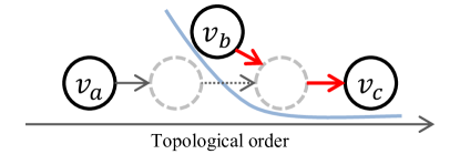
Figure 2: An illustration for the proof of Lemma 6.3.

Lemma 6.3.

Algorithm 7 has a separating dependence for the dependences and orderings $<_{v}$ defined above.

Proof.

By Definition 2, we need to show that for any three vertices $v_{a},v_{b},v_{c}\in V$, if $v_{a}<_{c}v_{b}<_{c}v_{c}$ or $v_{c}<_{c}v_{b}<_{c}v_{a}$, $v_{c}$ can only be reached (forward or backward) in $v_{a}$’s iteration if $v_{a}$’s iteration is the first among the three.

Clearly the statement is true if $v_{c}$ is earliest. We now consider the case when $v_{b}$’s iteration is first among the three vertices. We give the argument for the forward direction, and the backward direction is true by symmetry. If $v_{b}$ is in the same SCC as either $v_{a}$ or $v_{c}$, then in $v_{b}$’s iteration, either $v_{a}$ or $v_{c}$ is marked in one SCC that $v_{b}$ is in, and removed from the subgraph set ${\mathcal{V}}$. Otherwise, since $v_{b}$ and $v_{a}$ are not in the same SCC, when $v_{c}<_{c}v_{b}<_{c}v_{a}$, $v_{c}$ cannot be forward reachable in $v_{a}$’s iteration, and when $v_{a}<_{c}v_{b}<_{c}v_{c}$, $v_{a}$ cannot be forward reachable from $v_{b}$’s iteration. In the second case, after $v_{b}$’s iteration, the forward reachability search from $v_{b}$ reaches $v_{c}$ but not $v_{a}$, and so $v_{a}$ and $v_{c}$ fall into different components in ${\mathcal{V}}$ (shown in Figure 2). As a result, $v_{c}$ is also not reachable in $v_{a}$’s iteration.

In conclusion, $v_{c}$ can only be reached (forward or backward) in $v_{a}$’s iteration if $v_{a}$’s iteration is first among the three. ∎

This separating dependence implies that the sequential algorithm on a random ordering does $O(m\log n)$ work since each vertex $v_{j}$ is visited by no more than $\sum_{i=1}^{j}2/i=O(\log n)$ times in expectation shown by Lemma 2.3, and the upper bound of this expectation is independent of the degrees. Since $W_{R}(n,m)=O(m)$ sequentially, e.g., using BFS, this algorithm uses $O(m\log n)$ work on expectation.

We now consider the parallel version. We use the general approach of Type 3 algorithms as described in Section 2.3 and in particular Algorithm 2. The iterations we run in parallel for each round (consisting of increasing power of two) are the same as in Algorithm 7. To implement the parallel version, we need a way to efficiently combine the iterations that run in the same round. Based on our assumption, the reachability queries for each vertex in the round can run independently in parallel, and so we run the searches based on the partitioning of the vertices ${\mathcal{V}}$ from the previous round. For each direction, each search does a priority write with its ID in a temporary location to all the vertices it visits. We can then identify each strongly connected component by checking the reachability information on vertices. Vertices belonging in an SCC will have the ID of the highest priority search written in both of its temporary locations (one for each search direction), and vertices with the same ID written belong to the same SCC. To partition the graph, any edge between two vertices, where one is reachable and the other is not, in any of the reachability queries is cut. Each reachability search can identify and cut its own edges (some edges might be cut multiple times). This implementation is more aggressive than the the sequential algorithm, but this will only help. If required, the exact intermediate states of the sequential algorithm can also be maintained. After all $O(\log n)$ rounds are complete, we group the vertices to form SCCs based on their vertex labels. This requires linear work and $O(\log n)$ depth [58, 41].

Theorem 6.4.

For a random order of the input vertices, the incremental SCC algorithm does $O(W_{R}(n,m)\log n)$ expected work and has $O(D_{R}(n,m)\log n)$ depth on a priority-write CRCW PRAM.

Proof.

The overall extra work is $O(m\log n)$ and no more than the work for executing the reachability queries. The depth for the additional operations is constant in each round and $O(\log n)$ at the end of the algorithm. Therefore if the input vertices are randomly permuted, we can apply Theorem 2.6 with Lemma 6.3 and the convexity of the work cost to bound the expected work and depth of the algorithm. ∎

Acquiring the same intermediate states as the sequential algorithm. The partitioning of the vertex sets in previously discussed algorithm is more eager than the sequential algorithm. When determinism is needed, the same intermediate states in the sequential algorithm can be retrieved in the parallel version. Let’s consider the following case in one parallel round: vertex $z$ is forward reached from $x$ and reached from $y$, and at the meantime $x$ has a higher priority. The search of $y$ affects $z$ if and only if $y$ is also reached in $x$’s forward search. The other direction is symmetric.

With this observation, we can use the following algorithm to decide the partitioning of the vertices after one round in the sequential order. After the searches in each round finish, we first check whether each vertex is already in an SCC. For the vertices not in an SCC, we semisort pairs based on the source vertex of the search and the reached vertex, and gather all searches that reach each vertex in both directions. For each vertex, we then sort these searches based on the priorities of the source nodes, and use a scan to filter out the searches that do not reach this vertex in the sequential algorithm, based on the criteria above. Then the partitions are decided by the search with the lowest priority that reaches each vertex. Finally, we cut the edges based on the partitioning of the vertex sets using $O(m)$ work and constant depth. Using this approach guarantees the same intermediate states of the partitions at the end of each round compared to the sequential algorithm. The extra work in this step is the same as the post-processing in LE-lists in Section 6.1, which is dominated by the other parts in the algorithm.

7 Conclusion

In this paper, we have analyzed the dependence structure in a collection of known randomized incremental algorithms (or slight variants) and shown that there is inherently high parallelism in all of the algorithms. The approach leads to particularly simple parallel algorithms for the problems—only marginally more complicated (if at all) than some of the very simplest efficient sequential algorithms that are known for the problems. Furthermore the approach allows us to borrow much of the analysis already developed for the sequential versions (e.g., with regard to total work and correctness). We presented three general types of dependences of algorithms, and tools and general theorems that are useful for multiple algorithms within each type. We expect that there are many other algorithms that can be analyzed with these tools and theorems.

References

- [1] M. Ajtai and N. Megiddo. A deterministic -time -processor algorithm for linear programming in fixed dimension. In ACM Symposium on Theory of Computing (STOC), pages 327–338, 1992.
- [2] N. Alon and N. Megiddo. Parallel linear programming in fixed dimension almost surely in constant time. J. ACM, 41(2):422–434, Mar. 1994.
- [3] N. M. Amato, M. T. Goodrich, and E. A. Ramos. Parallel algorithms for higher-dimensional convex hulls. In Symposium on Foundations of Computer Science (FOCS), pages 683–694, 1994.
- [4] J. Barnat, P. Bauch, L. Brim, and M. Ceska. Computing strongly connected components in parallel on CUDA. In International Parallel & Distributed Processing Symposium (IPDPS), pages 544–555, 2011.
- [5] D. K. Blandford, G. E. Blelloch, and C. Kadow. Engineering a compact parallel Delaunay algorithm in 3D. In ACM Symposium on Computational Geometry (SoCG), pages 292–300, 2006.
- [6] G. E. Blelloch, J. T. Fineman, P. B. Gibbons, and J. Shun. Internally deterministic algorithms can be fast. In Principles and Practice of Parallel Programming (PPoPP), pages 181–192, 2012.
- [7] G. E. Blelloch, J. T. Fineman, and J. Shun. Greedy sequential maximal independent set and matching are parallel on average. In ACM Symposium on Parallelism in Algorithms and Architectures (SPAA), pages 308–317, 2012.
- [8] G. E. Blelloch, Y. Gu, and Y. Sun. Efficient construction of probabilistic tree embeddings. In International Colloquium on Automata, Languages and Programming (ICALP), 2017.
- [9] G. E. Blelloch, Y. Gu, Y. Sun, and K. Tangwongsan. Parallel shortest-paths using radius stepping. In ACM Symposium on Parallelism in Algorithms and Architectures (SPAA), 2016.
- [10] G. E. Blelloch, A. Gupta, and K. Tangwongsan. Parallel probabilistic tree embeddings, k-median, and buy-at-bulk network design. In ACM Symposium on Parallelism in Algorithms and Architectures (SPAA), pages 205–213, 2012.
- [11] G. E. Blelloch, J. C. Hardwick, G. L. Miller, and D. Talmor. Design and implementation of a practical parallel Delaunay algorithm. Algorithmica, 24(3-4):243–269, 1999.
- [12] R. L. Bocchino, V. S. Adve, S. V. Adve, and M. Snir. Parallel programming must be deterministic by default. In Usenix HotPar, 2009.
- [13] J.-D. Boissonnat and M. Teillaud. On the randomized construction of the delaunay tree. Theoretical Computer Science, 112(2):339–354, 1993.
- [14] R. P. Brent. The parallel evaluation of general arithmetic expressions. J. ACM (JACM), 21(2):201–206, 1974.
- [15] C. Cao Minh, J. Chung, C. Kozyrakis, and K. Olukotun. STAMP: Stanford transactional applications for multi-processing. In IEEE International Symposium on Workload Characterization (IISWC), 2008.
- [16] D. Z. Chen and J. Xu. Two-variable linear programming in parallel. Computational Geometry, 21(3):155 – 165, 2002.
- [17] P. Cignoni, C. Montani, R. Perego, and R. Scopigno. Parallel 3d delaunay triangulation. Computer Graphics Forum, 12(3):129–142, 1993.
- [18] M. Cintra, D. R. Llanos, and B. Palop. International conference on computational science and its applications. In Speculative Parallelization of a Randomized Incremental Convex Hull Algorithm, pages 188–197, 2004.
- [19] K. L. Clarkson and P. W. Shor. Applications of random sampling in computational geometry, II. Discrete & Computational Geometry, 4(5):387–421, 1989.
- [20] E. Cohen. Size-estimation framework with applications to transitive closure and reachability. Journal of Computer and System Sciences, 55(3):441–453, 1997.
- [21] E. Cohen and H. Kaplan. Efficient estimation algorithms for neighborhood variance and other moments. In ACM-SIAM Symposium on Discrete Algorithms (SODA), pages 157–166, 2004.
- [22] R. Cole. Parallel merge sort. SIAM J. Comput., 17(4):770–785, 1988.
- [23] R. Cole, M. T. Goodrich, and C. Ó. Dúnlaing. A nearly optimal deterministic parallel voronoi diagram algorithm. Algorithmica, 16(6):569–617, Dec 1996.
- [24] D. Coppersmith, L. Fleischer, B. Hendrickson, and A. Pinar. A divide-and-conquer algorithm for identifying strongly connected components. Technical Report RC23744, IBM, 2003.
- [25] T. H. Cormen, C. E. Leiserson, R. L. Rivest, and C. Stein. Introduction to Algorithms (3. ed.). MIT Press, 2009.
- [26] M. de Berg, O. Cheong, M. van Kreveld, and M. Overmars. Computational Geometry: Algorithms and Applications. Springer-Verlag, 2008.
- [27] X. Deng. An optimal parallel algorithm for linear programming in the plane. Information Processing Letters, 35(4):213 – 217, 1990.
- [28] L. Dhulipala, G. E. Blelloch, and J. Shun. Theoretically efficient parallel graph algorithms can be fast and scalable. In ACM Symposium on Parallelism in Algorithms and Architectures (SPAA), pages 393–404, 2018.
- [29] P. Diaz, D. R. Llanos, and B. Palop. Parallelizing 2D-convex hulls on clusters: Sorting matters. Jornadas De Paralelismo, 2004.
- [30] N. Du, L. Song, M. Gomez-Rodriguez, and H. Zha. Scalable influence estimation in continuous-time diffusion networks. In Advances in Neural Information Processing Systems (NIPS), pages 3147–3155, 2013.
- [31] M. Dyer. A parallel algorithm for linear programming in fixed dimension. In Symposium on Computational Geometry (SoCG), pages 345–349, 1995.
- [32] H. Edelsbrunner. Geometry and Topology for Mesh Generation. Cambridge University Press, 2006.
- [33] H. Edelsbrunner and N. R. Shah. Incremental topological flipping works for regular triangulations. Algorithmica, 15(3):223–241, 1996.
- [34] J. Fakcharoenphol, S. Rao, and K. Talwar. A tight bound on approximating arbitrary metrics by tree metrics. Journal of Computer and System Sciences (JCSS), 69(3):485–497, 2004.
- [35] J. Gil, Y. Matias, and U. Vishkin. Towards a theory of nearly constant time parallel algorithms. In Foundations of Computer Science (FOCS), pages 698–710, 1991.
- [36] M. Golin, R. Raman, C. Schwarz, and M. Smid. Simple randomized algorithms for closest pair problems. Nordic J. of Computing, 2(1):3–27, Mar. 1995.
- [37] A. Gonzalez-Escribano, D. R. Llanos, D. Orden, and B. Palop. Parallelization alternatives and their performance for the convex hull problem. Applied Mathematical Modelling, 30(7):563 – 577, 2006.
- [38] M. T. Goodrich. Fixed-dimensional parallel linear programming via relative -approximations. In ACM-SIAM Symposium on Discrete Algorithms (SODA), pages 132–141, 1996.
- [39] M. T. Goodrich and E. A. Ramos. Bounded-independence derandomization of geometric partitioning with applications to parallel fixed-dimensional linear programming. Discrete & Computational Geometry, 18(4):397–420, 1997.
- [40] P. J. Green and R. Sibson. Computing Dirichlet tessellations in the plane. The Computer Journal, 21(2):168–173, 1978.
- [41] Y. Gu, J. Shun, Y. Sun, and G. E. Blelloch. A top-down parallel semisort. In ACM Symposium on Parallelism in Algorithms and Architectures (SPAA), pages 24–34, 2015.
- [42] L. J. Guibas, D. E. Knuth, and M. Sharir. Randomized incremental construction of Delaunay and Voronoi diagrams. Algorithmica, 7(4):381–413, 1992.
- [43] T. Hagerup. Fast parallel generation of random permutations. In International Colloquium on Automata, Languages and Programming, pages 405–416. Springer, 1991.
- [44] S. Har-peled. Geometric Approximation Algorithms. American Mathematical Society, 2011.
- [45] W. Hasenplaugh, T. Kaler, T. B. Schardl, and C. E. Leiserson. Ordering heuristics for parallel graph coloring. In ACM Symposium on Parallelism in Algorithms and Architectures (SPAA), pages 166–177, 2014.
- [46] S. Hong, N. C. Rodia, and K. Olukotun. On fast parallel detection of strongly connected components (SCC) in small-world graphs. In International Conference for High Performance Computing, Networking, Storage and Analysis (SC), pages 1–11, 2013.
- [47] J. Jaja. Introduction to Parallel Algorithms. Addison-Wesley Professional, 1992.
- [48] S. Janson et al. Tail bounds for sums of geometric and exponential variables. Statistics & Probability Letters, 135(C):1–6, 2018.
- [49] M. Khan, F. Kuhn, D. Malkhi, G. Pandurangan, and K. Talwar. Efficient distributed approximation algorithms via probabilistic tree embeddings. Distributed Computing, 25(3):189–205, 2012.
- [50] S. Khuller and Y. Matias. A simple randomized sieve algorithm for the closest-pair problem. Information and Computation, 118(1):34–37, 1995.
- [51] P. N. Klein and S. Subramanian. A randomized parallel algorithm for single-source shortest paths. Journal of Algorithms, 25(2):205–220, 1997.
- [52] D. R. Llanos, D. Orden, and B. Palop. Meseta: A new scheduling strategy for speculative parallelization of randomized incremental algorithms. International Conference on Parallel Processing Workshops, pages 121–128, 2005.
- [53] N. Megiddo. Linear-time algorithms for linear programming in and related problems. SIAM Journal on Computing, 1983.
- [54] K. Mulmuley. Computational geometry - an introduction through randomized algorithms. Prentice Hall, 1994.
- [55] X. Pan, D. Papailiopoulos, S. Oymak, B. Recht, K. Ramchandran, and M. I. Jordan. Parallel correlation clustering on big graphs. In Advances in Neural Information Processing Systems (NIPS), 2015.
- [56] K. Pingali, D. Nguyen, M. Kulkarni, M. Burtscher, M. A. Hassaan, R. Kaleem, T.-H. Lee, A. Lenharth, R. Manevich, M. Méndez-Lojo, D. Prountzos, and X. Sui. The tao of parallelism in algorithms. In ACM SIGPLAN conference on Programming Language Design and Implementation (PLDI), 2011.
- [57] M. O. Rabin. Probabilistic algorithms. Algorithms and Complexity: New Directions and Recent Results, pages 21–39, 1976.
- [58] S. Rajasekaran and J. H. Reif. Optimal and sublogarithmic time randomized parallel sorting algorithms. SIAM J. Comput., 18(3):594–607, 1989.
- [59] J. H. Reif. Depth-first search is inherently sequential. Information Processing Letters, 20(5):229–234, 1985.
- [60] J. H. Reif and S. Sen. Optimal parallel randomized algorithms for three-dimensional convex hulls and related problems. SIAM J. Comput., 21(3):466–485, 1992.
- [61] W. Schudy. Finding strongly connected components in parallel using reachability queries. In ACM Symposium on Parallelism in Algorithms and Architectures (SPAA), pages 146–151, 2008.
- [62] R. Seidel. Small-dimensional linear programming and convex hulls made easy. Discrete & Computational Geometry, 6(3):423–434, 1991.
- [63] R. Seidel. Backwards analysis of randomized geometric algorithms. In New Trends in Discrete and Computational Geometry, pages 37–67. 1993.
- [64] S. Sen. A deterministic time optimal CRCW PRAM algorithm for linear programming in fixed dimensions. Technical report, Department of Computer Science, University of Newcastle, 1995.
- [65] J. Shun, G. E. Blelloch, J. T. Fineman, P. B. Gibbons, A. Kyrola, H. V. Simhadri, and K. Tangwongsan. Brief announcement: the Problem Based Benchmark Suite. In ACM Symposium on Parallelism in Algorithms and Architectures (SPAA), pages 68–70, 2012.
- [66] J. Shun, Y. Gu, G. Blelloch, J. Fineman, and P. Gibbons. Sequential random permutation, list contraction and tree contraction are highly parallel. In ACM-SIAM Symposium on Discrete Algorithms (SODA), pages 431–448, 2015.
- [67] G. M. Slota, S. Rajamanickam, and K. Madduri. BFS and Coloring-based parallel algorithms for strongly connected components and related problems. In International Parallel and Distributed Processing Symposium (IPDPS), 2014.
- [68] T. H. Spencer. Time-work tradeoffs for parallel algorithms. Journal of the ACM (JACM), 44(5):742–778, 1997.
- [69] R. Tarjan. Depth-first search and linear graph algorithms. SIAM Journal on Computing, 1(2):146–160, 1972.
- [70] D. Tomkins, T. Smith, N. M. Amato, and L. Rauchwerger. Efficient, reachability-based, parallel algorithms for finding strongly connected components. Technical report, Texas A&M University, 2015.
- [71] J. D. Ullman and M. Yannakakis. High-probability parallel transitive-closure algorithms. SIAM Journal on Computing, 20(1):100–125, 1991.
- [72] U. Vishkin. Thinking in parallel: Some basic data-parallel algorithms and techniques, 2010. Class notes from a course on parallel algorithms at UMD.
- [73] E. Welzl. Smallest enclosing disks (balls and ellipsoids). In New Results and New Trends in Computer Science, 1991.