Bilinear Factor Matrix Norm Minimization for Robust PCA: Algorithms and Applications

Fanhua Shang,  James Cheng, Yuanyuan Liu, Zhi-Quan Luo,  and Zhouchen Lin F. Shang (Corresponding author), J. Cheng and Y. Liu are with the Department of Computer Science and Engineering, The Chinese University of Hong Kong, Shatin, N.T., Hong Kong. E-mail: {fhshang, jcheng, yyliu}@cse.cuhk.edu.hk.Z.-Q. Luo is with Shenzhen Research Institute of Big Data, the Chinese University of Hong Kong, Shenzhen, China and Department of Electrical and Computer Engineering, University of Minnesota, Minneapolis, MN 55455, USA. E-mail: luozq@cuhk.edu.cn and luozq@umn.edu.Z. Lin is with Key Laboratory of Machine Perception (MOE), School of EECS, Peking University, Beijing 100871, P.R. China, and the Cooperative Medianet Innovation Center, Shanghai Jiao Tong University, Shanghai 200240, P.R. China. E-mail: zlin@pku.edu.cn.
Abstract

The heavy-tailed distributions of corrupted outliers and singular values of all channels in low-level vision have proven effective priors for many applications such as background modeling, photometric stereo and image alignment. And they can be well modeled by a hyper-Laplacian. However, the use of such distributions generally leads to challenging non-convex, non-smooth and non-Lipschitz problems, and makes existing algorithms very slow for large-scale applications. Together with the analytic solutions to psubscript𝑝\ell_{p}-norm minimization with two specific values of p𝑝p, i.e., p=1/2𝑝12p\!=\!1/2 and p=2/3𝑝23p\!=\!2/3, we propose two novel bilinear factor matrix norm minimization models for robust principal component analysis. We first define the double nuclear norm and Frobenius/nuclear hybrid norm penalties, and then prove that they are in essence the Schatten-1/2121/2 and 2/3232/3 quasi-norms, respectively, which lead to much more tractable and scalable Lipschitz optimization problems. Our experimental analysis shows that both our methods yield more accurate solutions than original Schatten quasi-norm minimization, even when the number of observations is very limited. Finally, we apply our penalties to various low-level vision problems, e.g., text removal, moving object detection, image alignment and inpainting, and show that our methods usually outperform the state-of-the-art methods.

Index Terms:
Robust principal component analysis, rank minimization, Schatten-p𝑝p quasi-norm, psubscript𝑝\ell_{p}-norm, double nuclear norm penalty, Frobenius/nuclear norm penalty, alternating direction method of multipliers (ADMM).

1 Introduction

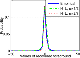
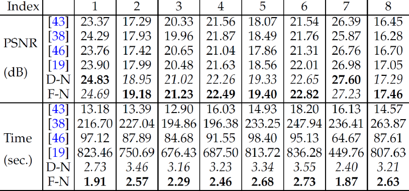
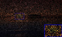
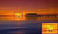
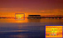
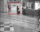
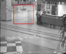
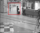
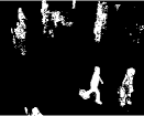
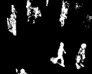
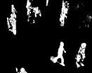
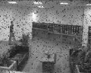
The sparse and low-rank priors have been widely used in many real-world applications in computer vision and pattern recognition, such as image restoration [1], face recognition [2], subspace clustering [3, 4, 5] and robust principal component analysis [6] (RPCA, also called low-rank and sparse matrix decomposition in [7, 8] or robust matrix completion in [9]). Sparsity plays an important role in various low-level vision tasks. For instance, it has been observed that the gradient of natural scene images can be better modeled with a heavy-tailed distribution such as hyper-Laplacian distributions (p(x)ek|x|αproportional-to𝑝𝑥superscript𝑒𝑘superscript𝑥𝛼p(x)\!\propto\!e^{-k|x|^{\alpha}}, typically with 0.5α0.80.5𝛼0.80.5\!\leq\!\alpha\!\leq\!0.8, which correspond to non-convex psubscript𝑝\ell_{p}-norms) [10, 11], as exhibited by the sparse noise/outliers in low-level vision problems [12] shown in Fig. 1. To induce sparsity, a principled way is to use the convex 1subscript1\ell_{1}-norm [6, 13, 14, 15, 16, 17], which is the closest convex relaxation of the sparser psubscript𝑝\ell_{p}-norm, with compressed sensing being a prominent example. However, it has been shown in [18] that the 1subscript1\ell_{1}-norm over-penalizes large entries of vectors and results in a biased solution. Compared with the 1subscript1\ell_{1}-norm, many non-convex surrogates of the 0subscript0\ell_{0}-norm listed in [19] give a closer approximation, e.g., SCAD [18] and MCP [20]. Although the use of hyper-Laplacian distributions makes the problems non-convex, fortunately an analytic solution can be derived for two specific values of p𝑝p, 1/2121/2 and 2/3232/3, by finding the roots of a cubic and quartic polynomial, respectively [10, 21, 22]. The resulting algorithm can be several orders of magnitude faster than existing algorithms [10].
Refer to caption
Refer to caption
Refer to caption
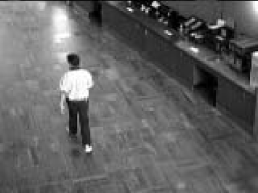
Figure 1: Sparsity priors. Left: A typical image of video sequences. Middle: the sparse component recovered by [6]. Right: the empirical distribution of the sparse component (blue solid line), along with a hyper-Laplacian fit with α=1/2𝛼12\alpha\!=\!1/2 (green dashdot line) and α=2/3𝛼23\alpha\!=\!2/3 (red dotted line).

As an extension from vectors to matrices, the low-rank structure is the sparsity of the singular values of a matrix. Rank minimization is a crucial regularizer to induce a low-rank solution. To solve such a problem, the rank function is usually relaxed by its convex envelope [5, 23, 24, 25, 26, 27, 28, 29], the nuclear norm (i.e., the sum of the singular values, also known as the trace norm or Schatten-111 norm [26, 30]). By realizing the intimate relationship between the 1subscript1\ell_{1}-norm and nuclear norm, the latter also over-penalizes large singular values, that is, it may make the solution deviate from the original solution as the 1subscript1\ell_{1}-norm does [19, 31]. Compared with the nuclear norm, the Schatten-q𝑞{q} norm for 0<q<10𝑞10\!<\!q\!<\!1 is equivalent to the qsubscript𝑞\ell_{q}-norm on singular values and makes a closer approximation to the rank function [32, 33]. Nie et al. [31] presented an efficient augmented Lagrange multiplier (ALM) method to solve the joint psubscript𝑝\ell_{p}-norm and Schatten-q𝑞q norm (LpSq) minimization. Lai et al. [32] and Lu et al. [33] proposed iteratively reweighted least squares methods for solving Schatten quasi-norm minimization problems. However, all these algorithms have to be solved iteratively, and involve singular value decomposition (SVD) in each iteration, which occupies the largest computation cost, 𝒪(min(m,n)mn)𝒪𝑚𝑛𝑚𝑛\mathcal{O}(\min(m,n)mn) [34, 35].

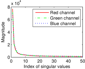
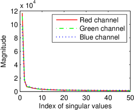
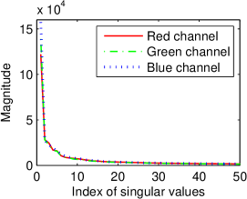
It has been shown in [36] that the singular values of nonlocal matrices in natural images usually exhibit a heavy-tailed distribution (p(σ)ek|σ|αproportional-to𝑝𝜎superscript𝑒𝑘superscript𝜎𝛼p(\sigma)\!\!\propto\!\!e^{-k|\sigma|^{\alpha}}), as well as the similar phenomena in natural scenes [37, 38], as shown in Fig. 2. Similar to the case of heavy-tailed distributions of sparse outliers, the analytic solutions can be derived for the two specific cases of α𝛼\alpha, 1/2121/2 and 2/3232/3. However, such algorithms have high per-iteration complexity 𝒪(min(m,n)mn)𝒪𝑚𝑛𝑚𝑛\mathcal{O}(\min(m,n)mn). Thus, we naturally want to design equivalent, tractable and scalable forms for the two cases of the Schatten-q𝑞q quasi-norm, q=1/2𝑞12q\!=\!1/2 and 2/3232/3, which can fit the heavy-tailed distribution of singular values closer than the nuclear norm, as analogous to the superiority of the psubscript𝑝\ell_{p} quasi-norm (hyper-Laplacian priors) to the 1subscript1\ell_{1}-norm (Laplacian priors).

Refer to caption
Refer to caption
Refer to caption
Refer to caption
Refer to caption
Refer to caption
Figure 2: The heavy-tailed empirical distributions (bottom) of the singular values of the three channels of these three images (top).

We summarize the main contributions of this work as follows. 1) By taking into account the heavy-tailed distributions of both sparse noise/outliers and singular values of matrices, we propose two novel tractable bilinear factor matrix norm minimization models for RPCA, which can fit empirical distributions very well to corrupted data. 2) Different from the definitions in our previous work [34], we define the double nuclear norm and Frobenius/nuclear hybrid norm penalties as tractable low-rank regularizers. Then we prove that they are in essence the Schatten-1/212{1/2} and 2/323{2/3} quasi-norms, respectively. The solution of the resulting minimization problems only requires SVDs on two much smaller factor matrices as compared with the much larger ones required by existing algorithms. Therefore, our algorithms can reduce the per-iteration complexity from 𝒪(min(m,n)mn)𝒪𝑚𝑛𝑚𝑛\mathcal{O}(\min(m,n)mn) to 𝒪(mnd)𝒪𝑚𝑛𝑑\mathcal{O}(mnd), where dm,nmuch-less-than𝑑𝑚𝑛d\!\ll\!m,n in general. In particular, our penalties are Lipschitz, and more tractable and scalable than original Schatten quasi-norm minimization, which is non-Lipschitz and generally NP-hard [32, 39]. 3) Moreover, we present the convergence property of the proposed algorithms for minimizing our RPCA models and provide their proofs. We also extend our algorithms to solve matrix completion problems, e.g., image inpainting. 4) We empirically study both of our bilinear factor matrix norm minimizations and show that they outperform original Schatten norm minimization, even with only a few observations. Finally, we apply the defined low-rank regularizers to address various low-level vision problems, e.g., text removal, moving object detection, and image alignment and inpainting, and obtain superior results than existing methods.

TABLE I: The norms of sparse and low-rank matrices. Let σ=(σ1,,σr)r𝜎subscript𝜎1subscript𝜎𝑟superscript𝑟\sigma\!=\!(\sigma_{1},\ldots,\sigma_{r})\!\in\!\mathbb{R}^{r} be the non-zero singular values of Lm×n𝐿superscript𝑚𝑛L\!\in\!\mathbb{R}^{m\!\times\!n}.
p,q𝑝𝑞\!p,q\! Sparsity Low-rankness
00\!0\! S0subscriptnorm𝑆subscript0\|S\|_{\ell_{0}} 0subscript0\!\ell_{0}-norm LS0=σ0subscriptnorm𝐿subscript𝑆0subscriptnorm𝜎subscript0\|L\|_{S_{0}}\!=\!\|\sigma\|_{\ell_{0}} ​​​rank
(0,1)01\!(0,1) Sp=(|Sij|p)1/psubscriptnorm𝑆subscript𝑝superscriptsuperscriptsubscript𝑆𝑖𝑗𝑝1𝑝\|S\|_{\ell_{p}}\!\!\!=\!\!(\!\sum\!|\!S_{ij}\!|^{p}\!)^{\!1\!/\!p}\!\! psubscript𝑝\!\ell_{p}-norm LSq=(σkq)1/qsubscriptnorm𝐿subscript𝑆𝑞superscriptsubscriptsuperscript𝜎𝑞𝑘1𝑞\|L\|_{\!S_{q}}\!\!\!=\!\!(\!\sum\!\sigma^{q}_{\!k}\!)^{\!1\!/\!q} ​​​Schatten-qSchatten-𝑞\textup{Schatten-}q norm​
11\!1\! S1=|Sij|subscriptnorm𝑆subscript1subscript𝑆𝑖𝑗\|S\|_{\ell_{1}}\!\!=\!\!\sum\!|S_{ij}| 1subscript1\!\ell_{1}-norm L=σksubscriptnorm𝐿subscript𝜎𝑘\|L\|_{*}\!\!=\!\!\sum\!\sigma_{k} ​​​nuclear norm
22\!2\! SF=Sij2subscriptnorm𝑆𝐹subscriptsuperscript𝑆2𝑖𝑗\|S\|_{\!F}\!=\!\sqrt{\sum\!S^{2}_{ij}} ​​​Frobenius norm LF=σk2subscriptnorm𝐿𝐹subscriptsuperscript𝜎2𝑘\|L\|_{\!F}\!=\!\sqrt{\sum\!\sigma^{2}_{k}} ​​Frobenius norm​​

2 Related Work

In this section, we mainly discuss some recent advances in RPCA, and briefly review some existing work on RPCA and its applications in computer vision (readers may see [6] for a review). RPCA [24, 40] aims to recover a low-rank matrix Lm×n𝐿superscript𝑚𝑛L\!\in\!\mathbb{R}^{m\times n} (mn𝑚𝑛m\!\geq\!n) and a sparse matrix Sm×n𝑆superscript𝑚𝑛S\!\in\!\mathbb{R}^{m\times n} from corrupted observations D=L+Sm×n𝐷superscript𝐿superscript𝑆superscript𝑚𝑛D\!=\!L^{*}\!+\!S^{*}\!\in\!\mathbb{R}^{m\times n} as follows:

minL,Sλrank(L)+S0,s.t.,L+S=Dsubscript𝐿𝑆𝜆rank𝐿subscriptnorm𝑆subscript0s.t.𝐿𝑆𝐷\min_{L,S}\;\lambda\,\textup{rank}(L)+\|S\|_{\ell_{0}},\;\textup{s.t.},L+S=D (1)

where 0\|\!\cdot\!\|_{\ell_{0}} denotes the 0subscript0\ell_{0}-norm111Strictly speaking, the 0subscript0\ell_{0}-norm is not actually a norm, and is defined as the number of non-zero elements. When p1𝑝1p\!\geq\!1, Spsubscriptnorm𝑆subscript𝑝\|S\|_{\ell_{p}} strictly defines a norm which satisfies the three norm conditions, while it defines a quasi-norm when 0<p<10𝑝10\!<\!p\!<\!1. Due to the relationship between Spsubscriptnorm𝑆subscript𝑝\|S\|_{\ell_{p}} and LSqsubscriptnorm𝐿subscript𝑆𝑞\|L\|_{\!S_{q}}, the latter has the same cases as the former. and λ>0𝜆0\lambda\!>\!0 is a regularization parameter. Unfortunately, solving (1) is NP-hard. Thus, we usually use the convex or non-convex surrogates to replace both of the terms in (1), and formulate this problem into the following more general form:

minL,SλLSqq+Spp,s.t.,𝒫Ω(L+S)=𝒫Ω(D)subscript𝐿𝑆𝜆subscriptsuperscriptnorm𝐿𝑞subscript𝑆𝑞subscriptsuperscriptnorm𝑆𝑝subscript𝑝s.t.subscript𝒫Ω𝐿𝑆subscript𝒫Ω𝐷\min_{L,S}\;\lambda\|L\|^{q}_{\!S_{q}}+\|S\|^{p}_{\ell_{p}},\;\textup{s.t.},\mathcal{P}_{\Omega}(L\!+\!S)=\mathcal{P}_{\Omega}(D) (2)

where in general p,q[0,2]𝑝𝑞02p,q\!\in\![0,2], Spsubscriptnorm𝑆subscript𝑝\|S\|_{\ell_{p}} and LSqsubscriptnorm𝐿subscript𝑆𝑞\|L\|_{\!S_{q}} are depicted in Table I and can be seen as the loss term and regularized term, respectively, and 𝒫Ωsubscript𝒫Ω\mathcal{P}_{\Omega} is the orthogonal projection onto the linear subspace of matrices supported on Ω:={(i,j)|Dijis observed}assignΩconditional-set𝑖𝑗subscript𝐷𝑖𝑗is observed\Omega\!:=\!\{(i,j)|D_{ij}\,\textup{is observed}\}: 𝒫Ω(D)ij=Dijsubscript𝒫Ωsubscript𝐷𝑖𝑗subscript𝐷𝑖𝑗\mathcal{P}_{\Omega}(D)_{ij}\!=\!D_{ij} if (i,j)Ω𝑖𝑗Ω(i,j)\!\in\!\Omega and 𝒫Ω(D)ij=0subscript𝒫Ωsubscript𝐷𝑖𝑗0\mathcal{P}_{\Omega}(D)_{ij}\!=\!0 otherwise. If ΩΩ\Omega is a small subset of the entries of the matrix, (2) is also known as the robust matrix completion problem as in [9], and it is impossible to exactly recover Ssuperscript𝑆{S}^{*} [41]. As analyzed in [42], we can easily see that the optimal solution SΩc=0subscript𝑆superscriptΩ𝑐0S_{\Omega^{c}}\!=\!\textbf{0}, where ΩcsuperscriptΩ𝑐\Omega^{c} is the complement of ΩΩ\Omega, i.e., the index set of unobserved entries. When p=2𝑝2p\!=\!2 and q=1𝑞1q\!=\!1, (2) becomes a nuclear norm regularized least squares problem as in [43] (e.g., image inpainting in Sec. 6.3.4).

TABLE II: Comparison of various RPCA models and their properties. Note that Um×d𝑈superscript𝑚𝑑U\!\in\!\mathbb{R}^{m\times d} and Vn×d𝑉superscript𝑛𝑑V\!\in\!\mathbb{R}^{n\times d} are the factor matrices of L𝐿L, i.e., L=UVT𝐿𝑈superscript𝑉𝑇L\!=\!UV^{T}.
Model Objective function Constraints Parameters Convex?​​ ​Per-iteration​​
​Complexity​​
RPCA [6, 44]​​​​ λL+S1𝜆subscriptnorm𝐿subscriptnorm𝑆subscript1\lambda\|L\|_{\ast}+\|S\|_{\ell_{1}} L+S=D𝐿𝑆𝐷L\!+\!S=D λ𝜆\lambda Yes 𝒪(mn2)𝒪𝑚superscript𝑛2\mathcal{O}(mn^{2})
PSVT [45] λLd+S1𝜆subscriptnorm𝐿𝑑subscriptnorm𝑆subscript1\lambda\|L\|_{d}+\|S\|_{\ell_{1}} L+S=D𝐿𝑆𝐷L\!+\!S=D λ,d𝜆𝑑\lambda,d No 𝒪(mn2)𝒪𝑚superscript𝑛2\mathcal{O}(mn^{2})
WNNM [46] λLw,+S1𝜆subscriptnorm𝐿𝑤subscriptnorm𝑆subscript1\lambda\|L\|_{w,*}+\|S\|_{\ell_{1}} λ𝜆\lambda
LMaFit [47] DL1subscriptnorm𝐷𝐿subscript1\|D\!-\!L\|_{\ell_{1}} UVT=L𝑈superscript𝑉𝑇𝐿UV^{T}\!=L d𝑑d No 𝒪(mnd)𝒪𝑚𝑛𝑑\mathcal{O}(mnd)
MTF [48] λW+S1𝜆subscriptnorm𝑊subscriptnorm𝑆subscript1\lambda\|W\|_{\ast}+\|S\|_{\ell_{1}} UWVT+S=D,UTU=VTV=Idformulae-sequence𝑈𝑊superscript𝑉𝑇𝑆𝐷superscript𝑈𝑇𝑈superscript𝑉𝑇𝑉subscript𝐼𝑑\!\!\!UWV^{T}\!\!\!+\!S\!=\!\!D,U^{T}\!U\!\!=\!\!V^{T}\!V\!\!=\!I_{d}\!\!\! λ,d𝜆𝑑\lambda,d
RegL1 [16]​​ λV+𝒫Ω(DUVT)1𝜆subscriptnorm𝑉subscriptnormsubscript𝒫Ω𝐷𝑈superscript𝑉𝑇subscript1\lambda\|V\|_{\ast}+\|\mathcal{P}_{\Omega}(D\!-\!UV^{T})\|_{\ell_{1}} UTU=Idsuperscript𝑈𝑇𝑈subscript𝐼𝑑U^{T}U\!=\!I_{d} λ,d𝜆𝑑\lambda,d
Unifying [49] λ2(UF2+VF2)+𝒫Ω(DL)1𝜆2subscriptsuperscriptnorm𝑈2𝐹subscriptsuperscriptnorm𝑉2𝐹subscriptnormsubscript𝒫Ω𝐷𝐿subscript1\frac{\lambda}{2}(\|U\|^{2}_{F}\!+\!\|V\|^{2}_{F})+\|\mathcal{P}_{\Omega}(D\!-\!L)\|_{\ell_{1}} UVT=L𝑈superscript𝑉𝑇𝐿UV^{T}\!=L λ,d𝜆𝑑\lambda,d
factEN [15] λ12(UF2+VF2)+λ22LF2+𝒫Ω(DL)1subscript𝜆12subscriptsuperscriptnorm𝑈2𝐹subscriptsuperscriptnorm𝑉2𝐹subscript𝜆22subscriptsuperscriptnorm𝐿2𝐹subscriptnormsubscript𝒫Ω𝐷𝐿subscript1\!\!\!\frac{\lambda_{1}}{2}\!(\|U\|^{2}_{F}\!\!+\!\!\|V\|^{2}_{F})\!+\!\!\frac{\lambda_{2}}{2}\!\|L\|^{2}_{F}\!\!+\!\!\|\mathcal{P}_{\Omega}(D\!-\!L)\|_{\ell_{1}}\!\!\! UVT=L𝑈superscript𝑉𝑇𝐿UV^{T}\!=L λ1,λ2,dsubscript𝜆1subscript𝜆2𝑑\lambda_{1},\lambda_{2},d
LpSq [31] λLSqq+𝒫Ω(DL)pp𝜆subscriptsuperscriptnorm𝐿𝑞subscript𝑆𝑞subscriptsuperscriptnormsubscript𝒫Ω𝐷𝐿𝑝subscript𝑝\lambda\|L\|^{q}_{\!S_{q}}\!+\!\|\mathcal{P}_{\Omega}(D\!-\!L)\|^{p}_{\ell_{p}} (0<p,q1)formulae-sequence0𝑝𝑞1(0\!<\!p,q\!\leq\!1) L+S=D𝐿𝑆𝐷L\!+\!S=D λ𝜆\lambda No 𝒪(mn2)𝒪𝑚superscript𝑛2\mathcal{O}(mn^{2})
(S+L)1/2subscriptS+L12\!(\textup{S+L})_{1/2} λ2(U+V)+𝒫Ω(S)1/21/2𝜆2subscriptnorm𝑈subscriptnorm𝑉subscriptsuperscriptnormsubscript𝒫Ω𝑆12subscript12\frac{\lambda}{2}(\|U\|_{*}\!+\!\|V\|_{*})+\|\mathcal{P}_{\Omega}(S)\|^{{1}/{2}}_{\ell_{{1}/{2}}} L+S=D,UVT=Lformulae-sequence𝐿𝑆𝐷𝑈superscript𝑉𝑇𝐿L\!+\!S\!=\!D,UV^{T}\!=L λ,d𝜆𝑑\lambda,d No 𝒪(mnd)𝒪𝑚𝑛𝑑\mathcal{O}(mnd)
(S+L)2/3subscriptS+L23\!(\textup{S+L})_{2/3} λ3(UF2+2V)+𝒫Ω(S)2/32/3𝜆3subscriptsuperscriptnorm𝑈2𝐹2subscriptnorm𝑉subscriptsuperscriptnormsubscript𝒫Ω𝑆23subscript23\frac{\lambda}{3}(\|U\|^{2}_{F}\!+\!2\|V\|_{*})+\|\mathcal{P}_{\Omega}(S)\|^{2/3}_{\ell_{{2}/{3}}}

2.1 Convex Nuclear Norm Minimization

In [6, 40, 44], both of the non-convex terms in (1) are replaced by their convex envelopes, i.e., the nuclear norm (q=1𝑞1q\!=\!1) and the 1subscript1\ell_{1}-norm (p=1𝑝1p\!=\!1), respectively.

minL,SλL+S1,s.t.,L+S=D.subscript𝐿𝑆𝜆subscriptnorm𝐿subscriptnorm𝑆subscript1s.t.𝐿𝑆𝐷\min_{L,S}\;\lambda\|L\|_{*}+\|S\|_{\ell_{1}},\;\textup{s.t.},L+S=D. (3)

Wright et al. [40] and Candès et al. [6] proved that, under some mild conditions, the convex relaxation formulation (3) can exactly recover the low-rank and sparse matrices (L,S)superscript𝐿superscript𝑆(L^{*},S^{*}) with high probability. The formulation (3) has been widely used in many computer vision applications, such as object detection and background subtraction [17], image alignment [50], low-rank texture analysis [29], image and video restoration [51], and subspace clustering [27]. This is mainly because the optimal solutions of the sub-problems involving both terms in (3) can be obtained by two well-known proximal operators: the singular value thresholding (SVT) operator [23] and the soft-thresholding operator [52]. The 1subscript1\ell_{1}-norm penalty in (3) can also be replaced by the 1,2subscript12\ell_{1,2}-norm as in outlier pursuit [28, 53, 54, 55] and subspace learning [5, 56, 57].

To efficiently solve the popular convex problem (3), various first-order optimization algorithms have been proposed, especially the alternating direction method of multipliers [58] (ADMM, or also called inexact ALM in [44]). However, they all involve computing the SVD of a large matrix of size m×n𝑚𝑛m\!\times\!n in each iteration, and thus suffer from high computational cost, which severely limits their applicability to large-scale problems [59], as well as existing Schatten-q𝑞q quasi-norm (0<q<10𝑞10\!<\!q\!<\!1) minimization algorithms such as LpSq [31]. While there have been many efforts towards fast SVD computation such as partial SVD [60], the performance of those methods is still unsatisfactory for many real applications [59, 61].

2.2 Non-Convex Formulations

To address this issue, Shen et al. [47] efficiently solved the RPCA problem by factorizing the low-rank component into two smaller factor matrices, i.e., L=UVT𝐿𝑈superscript𝑉𝑇L\!=\!UV^{T} as in [62], where Um×d𝑈superscript𝑚𝑑U\!\in\!\mathbb{R}^{m\times d}, Vn×d𝑉superscript𝑛𝑑V\!\in\!\mathbb{R}^{n\times d}, and usually dmin(m,n)much-less-than𝑑𝑚𝑛d\!\ll\!\min(m,n), as well as the matrix tri-factorization (MTF) [48] and factorized data [63] cases. In [16, 42, 64, 65, 66], the column-orthonormal constraint is imposed on the first factor matrix U𝑈U. According to the following matrix property, the original convex problem (3) can be reformulated as a smaller matrix nuclear norm minimization problem.

Property 1.

For any matrix Lm×n𝐿superscript𝑚𝑛L\!\in\!\mathbb{R}^{m\times n} and L=UVT𝐿𝑈superscript𝑉𝑇L\!=\!UV^{T}. If U𝑈U has orthonormal columns, i.e., UTU=Idsuperscript𝑈𝑇𝑈subscript𝐼𝑑U^{T}U\!=\!I_{d}, then L=Vsubscriptnorm𝐿subscriptnorm𝑉\|L\|_{*}\!=\!\|V\|_{*}.

Cabral et al. [49] and Kim et al. [15] replaced the nuclear norm regularizer in (3) with the equivalent non-convex formulation stated in Lemma 1, and proposed scalable bilinear spectral regularized models, similar to collaborative filtering applications in [26, 67]. In [15], an elastic-net regularized matrix factorization model was proposed for subspace learning and low-level vision problems.

Besides the popular nuclear norm, some variants of the nuclear norm were presented to yield better performance. Gu et al. [37] proposed a weighted nuclear norm (i.e., Lw,=iwiσisubscriptnorm𝐿𝑤subscript𝑖subscript𝑤𝑖subscript𝜎𝑖\|L\|_{w,*}\!=\!\sum_{i}\!w_{i}\sigma_{i}, where w=[w1,,wn]T𝑤superscriptsubscript𝑤1subscript𝑤𝑛𝑇w\!=\![w_{1},\ldots,w_{n}]^{T}), and assigned different weights wisubscript𝑤𝑖w_{i} to different singular values such that the shrinkage operator becomes more effective. Hu et al. [38] first used the truncated nuclear norm (i.e., Ld=i=d+1nσisubscriptnorm𝐿𝑑subscriptsuperscript𝑛𝑖𝑑1subscript𝜎𝑖\|L\|_{d}\!=\!\sum^{n}_{i=d+\!1}\!\sigma_{i}) to address image recovery problems. Subsequently, Oh et al. [45] proposed an efficient partial singular value thresholding (PSVT) algorithm to solve many RPCA problems of low-level vision. The formulations mentioned above are summarized in Table II.

3 Bilinear Factor Matrix Norm Minimization

In this section, we first define the double nuclear norm and Frobenius/nuclear hybrid norm penalties, and then prove the equivalence relationships between them and the Schatten quasi-norms. Incorporating with hyper-Laplacian priors of both sparse noise/outliers and singular values, we propose two novel bilinear factor matrix norm regularized models for RPCA. Although the two models are still non-convex and even non-smooth, they are more tractable and scalable optimization problems, and their each factor matrix term is convex. On the contrary, the original Schatten quasi-norm minimization problem is very difficult to solve because it is generally non-convex, non-smooth, and non-Lipschitz, as well as the qsubscript𝑞\ell_{q} quasi-norm [39].

As in some collaborative filtering applications [26, 67], the nuclear norm has the following alternative non-convex formulations.

Lemma 1.

For any matrix Xm×n𝑋superscript𝑚𝑛X\!\in\!\mathbb{R}^{m\times n} of rank at most rd𝑟𝑑r\leq d, the following equalities hold:

X=minUm×d,Vn×d:X=UVT12(UF2+VF2)=minU,V:X=UVTUFVF.subscriptdelimited-∥∥𝑋subscript:formulae-sequence𝑈superscript𝑚𝑑𝑉superscript𝑛𝑑𝑋𝑈superscript𝑉𝑇12subscriptsuperscriptdelimited-∥∥𝑈2𝐹subscriptsuperscriptdelimited-∥∥𝑉2𝐹subscript:𝑈𝑉𝑋𝑈superscript𝑉𝑇subscriptdelimited-∥∥𝑈𝐹subscriptdelimited-∥∥𝑉𝐹\begin{split}\|X\|_{*}&=\min_{U\in\mathbb{R}^{m\!\times\!d},V\in\mathbb{R}^{n\!\times\!d}:X=UV^{T}}\frac{1}{2}(\|U\|^{2}_{F}\!+\!\|V\|^{2}_{F})\\ &=\min_{U,V:X=UV^{T}}\|U\|_{F}\|V\|_{F}.\end{split} (4)

The bilinear spectral penalty in the first equality of (4) has been widely used in low-rank matrix completion and recovery problems, such as RPCA [15, 49], online RPCA [68], matrix completion [69], and image inpainting [25].

3.1 Double Nuclear Norm Penalty

Inspired by the equivalence relation between the nuclear norm and the bilinear spectral penalty, our double nuclear norm (D-N) penalty is defined as follows.

Definition 1.

For any matrix Xm×n𝑋superscript𝑚𝑛X\!\in\!\mathbb{R}^{m\times n} of rank at most rd𝑟𝑑r\leq d, we decompose it into two factor matrices Um×d𝑈superscript𝑚𝑑U\!\in\!\mathbb{R}^{m\times d} and Vn×d𝑉superscript𝑛𝑑V\!\in\!\mathbb{R}^{n\times d} such that X=UVT𝑋𝑈superscript𝑉𝑇X\!=\!UV^{T}. Then the double nuclear norm penalty of X𝑋X is defined as

XD-N=minU,V:X=UVT14(U+V)2.subscriptnorm𝑋D-Nsubscript:𝑈𝑉𝑋𝑈superscript𝑉𝑇14superscriptsubscriptnorm𝑈subscriptnorm𝑉2\|X\|_{\textup{D-N}}=\!\min_{U,V:X=UV^{T}}\frac{1}{4}(\|U\|_{*}\!+\!\|V\|_{*})^{2}. (5)

Different from the definition in [34, 70], i.e., minU,V:X=UVTUVsubscript:𝑈𝑉𝑋𝑈superscript𝑉𝑇subscriptnorm𝑈subscriptnorm𝑉\min_{U,V:X=UV^{T}}\|U\|_{*}\|V\|_{*}, which cannot be used directly to solve practical problems, Definition 1 can be directly used in practical low-rank matrix completion and recovery problems, e.g., RPCA and image recovery. Analogous to the well-known Schatten-q𝑞{q} quasi-norm [31, 32, 33], the double nuclear norm penalty is also a quasi-norm, and their relationship is stated in the following theorem.

Theorem 1.

The double nuclear norm penalty D-N\|\!\cdot\!\|_{\textup{D-N}} is a quasi-norm, and also the Schatten-1/212{1/2} quasi-norm, i.e.,

XD-N=XS1/2.subscriptnorm𝑋D-Nsubscriptnorm𝑋subscript𝑆12\|X\|_{\textup{D-N}}=\|X\|_{S_{1/2}}. (6)

To prove Theorem 1, we first give the following lemma, which is mainly used to extend the well-known trace inequality of John von Neumann [71, 72].

Lemma 2.

Let Xn×n𝑋superscript𝑛𝑛X\!\in\!\mathbb{R}^{n\times n} be a symmetric positive semi-definite (PSD) matrix and its full SVD be UXΣXUXTsubscript𝑈𝑋subscriptΣ𝑋subscriptsuperscript𝑈𝑇𝑋U_{X}\Sigma_{X}U^{T}_{X} with ΣX=diag(λ1,,λn)subscriptΣ𝑋diagsubscript𝜆1subscript𝜆𝑛\Sigma_{X}\!=\!\textup{diag}(\lambda_{1},\ldots,\lambda_{n}). Suppose Y𝑌Y is a diagonal matrix (i.e., Y=diag(τ1,,τn)𝑌diagsubscript𝜏1subscript𝜏𝑛Y\!=\!\textup{diag}(\tau_{1},\ldots,\tau_{n})), and if λ1λn0subscript𝜆1subscript𝜆𝑛0\lambda_{1}\!\geq\!\ldots\!\geq\!\lambda_{n}\!\geq\!0 and 0τ1τn0subscript𝜏1subscript𝜏𝑛0\!\leq\!\tau_{1}\!\leq\!\ldots\!\leq\!\tau_{n}, then

Tr(XTY)i=1nλiτi.Trsuperscript𝑋𝑇𝑌subscriptsuperscript𝑛𝑖1subscript𝜆𝑖subscript𝜏𝑖\textup{Tr}(X^{T}Y)\geq\sum^{n}_{i=1}\lambda_{i}\tau_{i}.

Lemma 2 can be seen as a special case of the well-known von Neumann’s trace inequality, and its proof is provided in the Supplementary Materials.

Lemma 3.

For any matrix X=UVTm×n𝑋𝑈superscript𝑉𝑇superscript𝑚𝑛X\!=\!{U}{V}^{T}\!\in\mathbb{R}^{m\times n}, Um×d𝑈superscript𝑚𝑑{U}\!\in\!\mathbb{R}^{m\times d} and Vn×d𝑉superscript𝑛𝑑{V}\!\in\!\mathbb{R}^{n\times d}, the following inequality holds:

12(U+V)XS1/21/2.12subscriptnorm𝑈subscriptnorm𝑉subscriptsuperscriptnorm𝑋12subscript𝑆12\frac{1}{2}\!\left(\|{U}\|_{*}+\|{V}\|_{*}\right)\geq\|X\|^{1/2}_{S_{1/2}}.
Proof:

Let U=LUΣURUT𝑈subscript𝐿𝑈subscriptΣ𝑈subscriptsuperscript𝑅𝑇𝑈U\!=\!L_{U}\Sigma_{U}R^{T}_{U} and V=LVΣVRVT𝑉subscript𝐿𝑉subscriptΣ𝑉subscriptsuperscript𝑅𝑇𝑉V\!=\!L_{V}\Sigma_{V}R^{T}_{V} be the thin SVDs of U𝑈U and V𝑉V, where LUm×dsubscript𝐿𝑈superscript𝑚𝑑L_{U}\!\in\!\mathbb{R}^{m\times d}, LVn×dsubscript𝐿𝑉superscript𝑛𝑑L_{V}\!\in\!\mathbb{R}^{n\times d}, and RU,ΣU,RV,ΣVd×dsubscript𝑅𝑈subscriptΣ𝑈subscript𝑅𝑉subscriptΣ𝑉superscript𝑑𝑑R_{U},\Sigma_{U},R_{V},\Sigma_{V}\!\in\!\mathbb{R}^{d\times d}. Let X=LXΣXRXT𝑋subscript𝐿𝑋subscriptΣ𝑋subscriptsuperscript𝑅𝑇𝑋X\!=\!L_{X}\Sigma_{X}R^{T}_{X}, where the columns of LXm×dsubscript𝐿𝑋superscript𝑚𝑑L_{X}\!\in\!\mathbb{R}^{m\times d} and RXn×dsubscript𝑅𝑋superscript𝑛𝑑R_{X}\!\in\!\mathbb{R}^{n\times d} are the left and right singular vectors associated with the top d𝑑d singular values of X𝑋X with rank at most r𝑟r (rd)𝑟𝑑(r\!\leq\!d), and ΣX=diag([σ1(X),,σr(X),0,,0])d×dsubscriptΣ𝑋diagsubscript𝜎1𝑋subscript𝜎𝑟𝑋00superscript𝑑𝑑\Sigma_{X}\!=\!\textup{diag}([\sigma_{1}(X),\!\cdots\!,\sigma_{r}(X),0,\!\cdots\!,0])\!\in\!\mathbb{R}^{d\times d}. Suppose W1=LXΣULXTsubscript𝑊1subscript𝐿𝑋subscriptΣ𝑈subscriptsuperscript𝐿𝑇𝑋W_{1}\!=\!L_{X}\Sigma_{U}L^{T}_{X}, W2=LXΣU12ΣX12LXTsubscript𝑊2subscript𝐿𝑋subscriptsuperscriptΣ12𝑈subscriptsuperscriptΣ12𝑋subscriptsuperscript𝐿𝑇𝑋W_{2}\!=\!L_{X}\Sigma^{\frac{1}{2}}_{U}\Sigma^{\frac{1}{2}}_{X}L^{T}_{X} and W3=LXΣXLXTsubscript𝑊3subscript𝐿𝑋subscriptΣ𝑋subscriptsuperscript𝐿𝑇𝑋W_{3}\!=\!L_{X}\Sigma_{X}L^{T}_{X}, we first construct the following PSD matrices 12m×2msubscript1superscript2𝑚2𝑚\mathcal{M}_{1}\!\in\!\mathbb{R}^{2m\times 2m} and 𝒮12m×2msubscript𝒮1superscript2𝑚2𝑚\mathcal{S}_{1}\!\in\!\mathbb{R}^{2m\times 2m}:

1=[LXΣU12LXΣX12][ΣU12LXTΣX12LXT]=[W1W2W2TW3]0,subscript1delimited-[]subscript𝐿𝑋subscriptsuperscriptΣ12𝑈subscript𝐿𝑋subscriptsuperscriptΣ12𝑋delimited-[]subscriptsuperscriptΣ12𝑈subscriptsuperscript𝐿𝑇𝑋subscriptsuperscriptΣ12𝑋subscriptsuperscript𝐿𝑇𝑋delimited-[]missing-subexpressionsubscript𝑊1subscript𝑊2missing-subexpressionsubscriptsuperscript𝑊𝑇2subscript𝑊3succeeds-or-equals0\mathcal{M}_{1}\!=\!\!\left[\begin{aligned} \!-L_{X}\Sigma^{\frac{1}{2}}_{U}\\ \!\!\!L_{X}\Sigma^{\frac{1}{2}}_{X}\!\end{aligned}\right]\!\!\left[\begin{aligned} -\Sigma^{\frac{1}{2}}_{U}L^{T}_{X}\;\Sigma^{\frac{1}{2}}_{X}L^{T}_{X}\end{aligned}\right]\!=\!\!\left[\begin{aligned} &\;\;W_{1}\quad\!\!-\!W_{2}\\ &\!\!-\!W^{T}_{2}\quad W_{3}\end{aligned}\right]\!\succeq\!0,
𝒮1=[InLUΣU12LUT][InLUΣU12LUT]=[InLUΣU12LUTLUΣU12LUTLUΣU1LUT]0.subscript𝒮1delimited-[]subscript𝐼𝑛subscript𝐿𝑈subscriptsuperscriptΣ12𝑈subscriptsuperscript𝐿𝑇𝑈delimited-[]subscript𝐼𝑛subscript𝐿𝑈subscriptsuperscriptΣ12𝑈subscriptsuperscript𝐿𝑇𝑈delimited-[]missing-subexpressionsubscript𝐼𝑛subscript𝐿𝑈subscriptsuperscriptΣ12𝑈subscriptsuperscript𝐿𝑇𝑈missing-subexpressionsubscript𝐿𝑈subscriptsuperscriptΣ12𝑈subscriptsuperscript𝐿𝑇𝑈subscript𝐿𝑈subscriptsuperscriptΣ1𝑈subscriptsuperscript𝐿𝑇𝑈succeeds-or-equals0\!\!\mathcal{S}_{1}\!=\!\!\left[\begin{aligned} \!I_{n}\qquad\\ \!L_{U}\!\Sigma^{-\!\frac{1}{2}}_{U}\!L^{T}_{U}\!\end{aligned}\right]\!\!\left[\begin{aligned} \!I_{n}\;L_{U}\!\Sigma^{-\!\frac{1}{2}}_{U}\!L^{T}_{U}\!\end{aligned}\right]\!\!=\!\!\!\left[\begin{aligned} &\quad\;I_{n}\;\;\;\quad\;L_{U}\!\Sigma^{-\!\frac{1}{2}}_{U}\!L^{T}_{U}\\ &\!L_{U}\!\Sigma^{-\!\frac{1}{2}}_{U}\!L^{T}_{U}\;L_{U}\!\Sigma^{-\!1}_{U}\!L^{T}_{U}\!\end{aligned}\right]\!\!\succeq\!\!0.

Because the trace of the product of two PSD matrices is always non-negative (see the proof of Lemma 6 in [73]), we have

Tr([InLUΣU12LUTLUΣU12LUTLUΣU1LUT][W1W2W2TW3])0.Trdelimited-[]missing-subexpressionsubscript𝐼𝑛subscript𝐿𝑈subscriptsuperscriptΣ12𝑈subscriptsuperscript𝐿𝑇𝑈missing-subexpressionsubscript𝐿𝑈subscriptsuperscriptΣ12𝑈subscriptsuperscript𝐿𝑇𝑈subscript𝐿𝑈subscriptsuperscriptΣ1𝑈subscriptsuperscript𝐿𝑇𝑈delimited-[]missing-subexpressionsubscript𝑊1subscript𝑊2missing-subexpressionsubscriptsuperscript𝑊𝑇2subscript𝑊30\begin{split}\textrm{Tr}\left(\left[\begin{aligned} &\quad\;I_{n}\;\;\;\quad\;L_{U}\!\Sigma^{-\frac{1}{2}}_{U}\!L^{T}_{U}\\ &\!L_{U}\!\Sigma^{-\frac{1}{2}}_{U}\!L^{T}_{U}\;L_{U}\!\Sigma^{-1}_{U}\!L^{T}_{U}\end{aligned}\right]\!\left[\begin{aligned} &\;\;W_{1}\quad\!\!-\!W_{2}\\ &\!\!-\!W^{T}_{2}\quad W_{3}\end{aligned}\right]\right)\geq 0.\end{split}

By further simplifying the above expression, we obtain

Tr(W1)2Tr(LUΣU12LUTW2T)+Tr(LUΣU1LUTW3)0.Trsubscript𝑊12Trsubscript𝐿𝑈subscriptsuperscriptΣ12𝑈subscriptsuperscript𝐿𝑇𝑈subscriptsuperscript𝑊𝑇2Trsubscript𝐿𝑈subscriptsuperscriptΣ1𝑈subscriptsuperscript𝐿𝑇𝑈subscript𝑊30\textrm{Tr}(W_{1})\!-\!2\textrm{Tr}(L_{U}\!\Sigma^{-\frac{1}{2}}_{U}\!L^{T}_{U}\!W^{T}_{2})\!+\!\textrm{Tr}(L_{U}\!\Sigma^{-1}_{U}\!L^{T}_{U}\!W_{3})\!\geq\!0. (7)

Recalling X=UVT𝑋𝑈superscript𝑉𝑇X\!=\!UV^{T} and LXΣXRXT=LUΣURUTRVΣVLVTsubscript𝐿𝑋subscriptΣ𝑋subscriptsuperscript𝑅𝑇𝑋subscript𝐿𝑈subscriptΣ𝑈subscriptsuperscript𝑅𝑇𝑈subscript𝑅𝑉subscriptΣ𝑉subscriptsuperscript𝐿𝑇𝑉L_{X}\!\Sigma_{X}\!R^{T}_{X}\!=\!L_{U}\!\Sigma_{U}\!R^{T}_{U}\!R_{V}\!\Sigma_{V}\!L^{T}_{V}, thus LUTLXΣX=ΣURUTRVΣVLVTRXsubscriptsuperscript𝐿𝑇𝑈subscript𝐿𝑋subscriptΣ𝑋subscriptΣ𝑈subscriptsuperscript𝑅𝑇𝑈subscript𝑅𝑉subscriptΣ𝑉subscriptsuperscript𝐿𝑇𝑉subscript𝑅𝑋L^{T}_{U}\!L_{X}\!\Sigma_{X}\!=\!\Sigma_{U}\!R^{T}_{U}\!R_{V}\!\Sigma_{V}\!L^{T}_{V}\!R_{X}. Due to the orthonormality of the columns of LUsubscript𝐿𝑈L_{U}, RUsubscript𝑅𝑈R_{U}, LVsubscript𝐿𝑉L_{V}, RVsubscript𝑅𝑉R_{V}, LXsubscript𝐿𝑋L_{X} and RXsubscript𝑅𝑋R_{X}, and using the well-known von Neumann’s trace inequality [71, 72], we obtain

Tr(LUΣU1LUTW3)=Tr(LUΣU1LUTLXΣXLXT)=Tr(LUΣU1ΣURUTRVΣVLVTRXLXT)=Tr(LURUTRVΣVLVTRXLXT)Tr(ΣV)=V.Trsubscript𝐿𝑈subscriptsuperscriptΣ1𝑈subscriptsuperscript𝐿𝑇𝑈subscript𝑊3Trsubscript𝐿𝑈subscriptsuperscriptΣ1𝑈subscriptsuperscript𝐿𝑇𝑈subscript𝐿𝑋subscriptΣ𝑋subscriptsuperscript𝐿𝑇𝑋Trsubscript𝐿𝑈subscriptsuperscriptΣ1𝑈subscriptΣ𝑈subscriptsuperscript𝑅𝑇𝑈subscript𝑅𝑉subscriptΣ𝑉subscriptsuperscript𝐿𝑇𝑉subscript𝑅𝑋subscriptsuperscript𝐿𝑇𝑋Trsubscript𝐿𝑈subscriptsuperscript𝑅𝑇𝑈subscript𝑅𝑉subscriptΣ𝑉subscriptsuperscript𝐿𝑇𝑉subscript𝑅𝑋subscriptsuperscript𝐿𝑇𝑋TrsubscriptΣ𝑉subscriptdelimited-∥∥𝑉\begin{split}&\,\textrm{Tr}(L_{U}\Sigma^{-1}_{U}L^{T}_{U}W_{3})=\textrm{Tr}(L_{U}\Sigma^{-1}_{U}L^{T}_{U}L_{X}\Sigma_{X}L^{T}_{X})\\ =&\,\textrm{Tr}(L_{U}\Sigma^{-1}_{U}\Sigma_{U}R^{T}_{U}R_{V}\Sigma_{V}L^{T}_{V}R_{X}L^{T}_{X})\\ =&\,\textrm{Tr}(L_{U}R^{T}_{U}R_{V}\Sigma_{V}L^{T}_{V}R_{X}L^{T}_{X})\\ \leq&\,\textrm{Tr}(\Sigma_{V})=\|V\|_{*}.\end{split} (8)

Using Lemma 2, we have

Tr(LUΣU12LUTW2T)=Tr(LUΣU12LUTLXΣU12ΣX12LXT)=Tr(ΣU12LUTLXΣU12ΣX12LXTLU)=Tr(ΣU12O1ΣU12ΣX12O1T)Tr(ΣU12ΣU12ΣX12)=Tr(ΣX12)=XS1/21/2Trsubscript𝐿𝑈subscriptsuperscriptΣ12𝑈subscriptsuperscript𝐿𝑇𝑈subscriptsuperscript𝑊𝑇2Trsubscript𝐿𝑈subscriptsuperscriptΣ12𝑈subscriptsuperscript𝐿𝑇𝑈subscript𝐿𝑋subscriptsuperscriptΣ12𝑈subscriptsuperscriptΣ12𝑋subscriptsuperscript𝐿𝑇𝑋TrsubscriptsuperscriptΣ12𝑈subscriptsuperscript𝐿𝑇𝑈subscript𝐿𝑋subscriptsuperscriptΣ12𝑈subscriptsuperscriptΣ12𝑋subscriptsuperscript𝐿𝑇𝑋subscript𝐿𝑈TrsubscriptsuperscriptΣ12𝑈subscript𝑂1subscriptsuperscriptΣ12𝑈subscriptsuperscriptΣ12𝑋subscriptsuperscript𝑂𝑇1TrsubscriptsuperscriptΣ12𝑈subscriptsuperscriptΣ12𝑈subscriptsuperscriptΣ12𝑋TrsubscriptsuperscriptΣ12𝑋subscriptsuperscriptdelimited-∥∥𝑋12subscript𝑆12\begin{split}&\,\textrm{Tr}(\!L_{U}\!\Sigma^{-\frac{1}{2}}_{U}\!L^{T}_{U}\!W^{T}_{2})\!=\!\textrm{Tr}(\!L_{U}\!\Sigma^{-\frac{1}{2}}_{U}\!L^{T}_{U}\!L_{X}\!\Sigma^{\frac{1}{2}}_{U}\!\Sigma^{\frac{1}{2}}_{X}\!L^{T}_{X})\\ =&\,\textrm{Tr}(\Sigma^{-\frac{1}{2}}_{U}L^{T}_{U}L_{X}\Sigma^{\frac{1}{2}}_{U}\Sigma^{\frac{1}{2}}_{X}L^{T}_{X}L_{U})\\ =&\,\textrm{Tr}(\Sigma^{-\frac{1}{2}}_{U}O_{1}\Sigma^{\frac{1}{2}}_{U}\Sigma^{\frac{1}{2}}_{X}O^{T}_{1})\\ \geq&\,\textrm{Tr}(\Sigma^{-\frac{1}{2}}_{U}\Sigma^{\frac{1}{2}}_{U}\Sigma^{\frac{1}{2}}_{X})=\textrm{Tr}(\Sigma^{\frac{1}{2}}_{X})=\|X\|^{1/2}_{S_{1/2}}\end{split} (9)

where O1=LUTLXd×dsubscript𝑂1subscriptsuperscript𝐿𝑇𝑈subscript𝐿𝑋superscript𝑑𝑑O_{1}\!=\!L^{T}_{U}L_{X}\in\mathbb{R}^{d\times d}, and it is easy to verify that O1ΣU12ΣX12O1Tsubscript𝑂1subscriptsuperscriptΣ12𝑈subscriptsuperscriptΣ12𝑋subscriptsuperscript𝑂𝑇1O_{1}\Sigma^{\frac{1}{2}}_{U}\Sigma^{\frac{1}{2}}_{X}O^{T}_{1} is a symmetric PSD matrix. Using (7), (44), (45) and Tr(W1)=UTrsubscript𝑊1subscriptnorm𝑈\textrm{Tr}(W_{1})\!=\!\|U\|_{*}, we have U+V2XS1/21/2subscriptnorm𝑈subscriptnorm𝑉2subscriptsuperscriptnorm𝑋12subscript𝑆12\|U\|_{*}\!+\!\|V\|_{*}\geq 2\|X\|^{1/2}_{S_{1/2}}. ∎

The detailed proof of Theorem 1 is provided in the Supplementary Materials. According to Theorem 1, it is easy to verify that the double nuclear norm penalty possesses the following property [34].

Property 2.

Given a matrix Xm×n𝑋superscript𝑚𝑛X\!\in\!\mathbb{R}^{m\times n} with rank(X)drank𝑋𝑑\textrm{rank}(X)\!\leq\!d, the following equalities hold:

XD-N=minUm×d,Vn×d:X=UVT(U+V2)2=minU,V:X=UVTUV.\begin{split}\|X\|_{\textup{D-N}}&=\min_{U\in\mathbb{R}^{m\!\times\!d},V\in\mathbb{R}^{n\!\times\!d}:X=UV^{T}}\left(\frac{\|U\|_{*}\!+\!\|V\|_{*}}{2}\right)^{2}\\ &=\min_{U,V:X=UV^{T}}\!\|U\|_{*}\|V\|_{*}.\end{split}

3.2 Frobenius/Nuclear Norm Penalty

Inspired by the definitions of the bilinear spectral and double nuclear norm penalties mentioned above, we define a Frobenius/nuclear hybrid norm (F-N) penalty as follows.

Definition 2.

For any matrix Xm×n𝑋superscript𝑚𝑛X\!\in\!\mathbb{R}^{m\times n} of rank at most rd𝑟𝑑r\leq d, we decompose it into two factor matrices Um×d𝑈superscript𝑚𝑑U\!\in\!\mathbb{R}^{m\times d} and Vn×d𝑉superscript𝑛𝑑V\!\in\!\mathbb{R}^{n\times d} such that X=UVT𝑋𝑈superscript𝑉𝑇X\!=\!UV^{T}. Then the Frobenius/nuclear hybrid norm penalty of X𝑋X is defined as

XF-N=minU,V:X=UVT[(UF2+2V)/3]3/2.\|X\|_{\textup{F-N}}=\!\min_{U,V:X=UV^{T}}\,\left[(\|U\|^{2}_{F}\!+\!2\|V\|_{*})/3\right]^{3/2}. (10)

Different from the definition in [34], i.e., minU,V:X=UVTUFVsubscript:𝑈𝑉𝑋𝑈superscript𝑉𝑇subscriptnorm𝑈𝐹subscriptnorm𝑉\min_{U,V:X=UV^{T}}\!\|U\|_{F}\|V\|_{*}, Definition 2 can also be directly used in practical problems. Analogous to the double nuclear norm penalty, the Frobenius/nuclear hybrid norm penalty is also a quasi-norm, as stated in the following theorem.

Theorem 2.

The Frobenius/nuclear hybrid norm penalty, F-N\|\!\cdot\!\|_{\textup{F-N}}, is a quasi-norm, and is also the Schatten-2/323{2/3} quasi-norm, i.e.,

XF-N=XS2/3.subscriptnorm𝑋F-Nsubscriptnorm𝑋subscript𝑆23\|X\|_{\textup{F-N}}=\|X\|_{S_{2/3}}. (11)

To prove Theorem 2, we first give the following lemma.

Lemma 4.

For any matrix X=UVTm×n𝑋𝑈superscript𝑉𝑇superscript𝑚𝑛X\!=\!{U}{V}^{T}\!\in\!\mathbb{R}^{m\times n}, Um×d𝑈superscript𝑚𝑑{U}\!\in\!\mathbb{R}^{m\times d} and Vn×d𝑉superscript𝑛𝑑{V}\!\in\!\mathbb{R}^{n\times d}, the following inequality holds:

13(UF2+2V)XS2/32/3.13subscriptsuperscriptnorm𝑈2𝐹2subscriptnorm𝑉subscriptsuperscriptnorm𝑋23subscript𝑆23\frac{1}{3}\!\left(\|{U}\|^{2}_{F}+2\|{V}\|_{*}\right)\geq\|X\|^{2/3}_{S_{2/3}}.
Proof:

To prove this lemma, we use the same notations as in the proof of Lemma 3, e.g., X=LXΣXRXT𝑋subscript𝐿𝑋subscriptΣ𝑋subscriptsuperscript𝑅𝑇𝑋X\!=\!L_{X}\Sigma_{X}R^{T}_{X}, U=LUΣURUT𝑈subscript𝐿𝑈subscriptΣ𝑈subscriptsuperscript𝑅𝑇𝑈U\!=\!L_{U}\Sigma_{U}R^{T}_{U} and V=LVΣVRVT𝑉subscript𝐿𝑉subscriptΣ𝑉subscriptsuperscript𝑅𝑇𝑉V\!=\!L_{V}\Sigma_{V}R^{T}_{V} denote the thin SVDs of U𝑈U and V𝑉V, respectively. Suppose W¯1=RXΣVRXTsubscript¯𝑊1subscript𝑅𝑋subscriptΣ𝑉subscriptsuperscript𝑅𝑇𝑋\overline{W}_{\!1}\!=\!R_{X}\Sigma_{V}R^{T}_{X}, W¯2=RXΣV12ΣX23RXTsubscript¯𝑊2subscript𝑅𝑋subscriptsuperscriptΣ12𝑉subscriptsuperscriptΣ23𝑋subscriptsuperscript𝑅𝑇𝑋\overline{W}_{\!2}\!=\!R_{X}\Sigma^{\frac{1}{2}}_{V}\Sigma^{\frac{2}{3}}_{X}R^{T}_{X} and W¯3=RXΣX43RXTsubscript¯𝑊3subscript𝑅𝑋subscriptsuperscriptΣ43𝑋subscriptsuperscript𝑅𝑇𝑋\overline{W}_{\!3}\!=\!R_{X}\Sigma^{\frac{4}{3}}_{X}R^{T}_{X}, we first construct the following PSD matrices 22m×2msubscript2superscript2𝑚2𝑚\mathcal{M}_{2}\!\in\!\mathbb{R}^{2m\times 2m} and 𝒮22m×2msubscript𝒮2superscript2𝑚2𝑚\mathcal{S}_{2}\!\in\!\mathbb{R}^{2m\times 2m}:

2=[RXΣV12RXΣX23][ΣV12RXTΣX23RXT]=[W¯1W¯2W¯2TW¯3]0,subscript2delimited-[]subscript𝑅𝑋subscriptsuperscriptΣ12𝑉subscript𝑅𝑋subscriptsuperscriptΣ23𝑋delimited-[]subscriptsuperscriptΣ12𝑉subscriptsuperscript𝑅𝑇𝑋subscriptsuperscriptΣ23𝑋subscriptsuperscript𝑅𝑇𝑋delimited-[]missing-subexpressionsubscript¯𝑊1subscript¯𝑊2missing-subexpressionsubscriptsuperscript¯𝑊𝑇2subscript¯𝑊3succeeds-or-equals0\mathcal{M}_{2}\!=\!\!\left[\begin{aligned} \!-R_{X}\Sigma^{\frac{1}{2}}_{V}\\ \!\!\!R_{X}\Sigma^{\frac{2}{3}}_{X}\!\end{aligned}\right]\!\!\left[\begin{aligned} -\Sigma^{\frac{1}{2}}_{V}R^{T}_{X}\;\Sigma^{\frac{2}{3}}_{X}R^{T}_{X}\end{aligned}\right]\!=\!\!\left[\begin{aligned} &\;\;\overline{W}_{\!1}\quad\!\!-\!\overline{W}_{\!2}\\ &\!\!-\!\overline{W}^{T}_{\!2}\quad\overline{W}_{\!3}\end{aligned}\right]\!\succeq\!0,
𝒮2=[InLVΣV12LVT][InLVΣV12LVT]=[InLVΣV12LVTLVΣV12LVTLVΣV1LVT]0.subscript𝒮2delimited-[]subscript𝐼𝑛subscript𝐿𝑉subscriptsuperscriptΣ12𝑉subscriptsuperscript𝐿𝑇𝑉delimited-[]subscript𝐼𝑛subscript𝐿𝑉subscriptsuperscriptΣ12𝑉subscriptsuperscript𝐿𝑇𝑉delimited-[]missing-subexpressionsubscript𝐼𝑛subscript𝐿𝑉subscriptsuperscriptΣ12𝑉subscriptsuperscript𝐿𝑇𝑉missing-subexpressionsubscript𝐿𝑉subscriptsuperscriptΣ12𝑉subscriptsuperscript𝐿𝑇𝑉subscript𝐿𝑉subscriptsuperscriptΣ1𝑉subscriptsuperscript𝐿𝑇𝑉succeeds-or-equals0\!\!\mathcal{S}_{2}\!=\!\!\left[\begin{aligned} \!I_{n}\qquad\\ \!L_{V}\!\Sigma^{-\!\frac{1}{2}}_{V}\!L^{T}_{V}\!\end{aligned}\right]\!\!\left[\begin{aligned} \!I_{n}\;L_{V}\!\Sigma^{-\!\frac{1}{2}}_{V}\!L^{T}_{V}\!\end{aligned}\right]\!\!=\!\!\left[\begin{aligned} &\quad\;I_{n}\;\;\;\quad\;L_{V}\!\Sigma^{-\!\frac{1}{2}}_{V}\!L^{T}_{V}\\ &\!L_{V}\!\Sigma^{-\!\frac{1}{2}}_{V}\!L^{T}_{V}\;L_{V}\!\Sigma^{-\!1}_{V}\!L^{T}_{V}\!\end{aligned}\right]\!\!\succeq\!\!0.

Similar to Lemma 3, we have the following inequality:

Tr([InLVΣV12LVTLVΣV12LVTLVΣV1LVT][W¯1W¯2W¯2TW¯3])0.Trdelimited-[]missing-subexpressionsubscript𝐼𝑛subscript𝐿𝑉subscriptsuperscriptΣ12𝑉subscriptsuperscript𝐿𝑇𝑉missing-subexpressionsubscript𝐿𝑉subscriptsuperscriptΣ12𝑉subscriptsuperscript𝐿𝑇𝑉subscript𝐿𝑉subscriptsuperscriptΣ1𝑉subscriptsuperscript𝐿𝑇𝑉delimited-[]missing-subexpressionsubscript¯𝑊1subscript¯𝑊2missing-subexpressionsubscriptsuperscript¯𝑊𝑇2subscript¯𝑊30\begin{split}\textrm{Tr}\left(\left[\begin{aligned} &\quad\;I_{n}\;\;\;\quad\;L_{V}\!\Sigma^{-\frac{1}{2}}_{V}\!L^{T}_{V}\\ &\!L_{V}\!\Sigma^{-\frac{1}{2}}_{V}\!L^{T}_{V}\;L_{V}\!\Sigma^{-1}_{V}\!L^{T}_{V}\end{aligned}\right]\!\left[\begin{aligned} &\;\;\overline{W}_{\!1}\quad\!\!-\!\overline{W}_{\!2}\\ &\!\!-\!\overline{W}^{T}_{\!2}\quad\overline{W}_{\!3}\end{aligned}\right]\right)\geq 0.\end{split}

By further simplifying the above expression, we also obtain

Tr(W¯1)2Tr(LVΣV12LVTW¯2T)+Tr(LVΣV1LVTW¯3)0.Trsubscript¯𝑊12Trsubscript𝐿𝑉subscriptsuperscriptΣ12𝑉subscriptsuperscript𝐿𝑇𝑉subscriptsuperscript¯𝑊𝑇2Trsubscript𝐿𝑉subscriptsuperscriptΣ1𝑉subscriptsuperscript𝐿𝑇𝑉subscript¯𝑊30\textrm{Tr}(\overline{W}_{\!1})-2\textrm{Tr}(L_{V}\!\Sigma^{-\frac{1}{2}}_{V}\!L^{T}_{V}\overline{W}^{T}_{\!2})+\textrm{Tr}(L_{V}\!\Sigma^{-1}_{V}\!L^{T}_{V}\overline{W}_{\!3})\geq 0. (12)

Since LXΣXRXT=LUΣURUTRVΣVLVTsubscript𝐿𝑋subscriptΣ𝑋subscriptsuperscript𝑅𝑇𝑋subscript𝐿𝑈subscriptΣ𝑈subscriptsuperscript𝑅𝑇𝑈subscript𝑅𝑉subscriptΣ𝑉subscriptsuperscript𝐿𝑇𝑉L_{X}\Sigma_{X}R^{T}_{X}\!=\!L_{U}\Sigma_{U}R^{T}_{U}R_{V}\Sigma_{V}L^{T}_{V}, LVTRXΣX=(LXTLUΣURUTRVΣV)T=ΣVRVTRUΣULUTLXsubscriptsuperscript𝐿𝑇𝑉subscript𝑅𝑋subscriptΣ𝑋superscriptsubscriptsuperscript𝐿𝑇𝑋subscript𝐿𝑈subscriptΣ𝑈subscriptsuperscript𝑅𝑇𝑈subscript𝑅𝑉subscriptΣ𝑉𝑇subscriptΣ𝑉subscriptsuperscript𝑅𝑇𝑉subscript𝑅𝑈subscriptΣ𝑈subscriptsuperscript𝐿𝑇𝑈subscript𝐿𝑋L^{T}_{V}R_{X}\Sigma_{X}\!=\!(L^{T}_{X}L_{U}\Sigma_{U}R^{T}_{U}R_{V}\Sigma_{V})^{T}\!=\!\Sigma_{V}R^{T}_{V}R_{U}\Sigma_{U}L^{T}_{U}L_{X}. Due to the orthonormality of the columns of LUsubscript𝐿𝑈L_{U}, RUsubscript𝑅𝑈R_{U}, LVsubscript𝐿𝑉L_{V}, RVsubscript𝑅𝑉R_{V}, LXsubscript𝐿𝑋L_{X} and RXsubscript𝑅𝑋R_{X}, and using the von Neumann’s trace inequality [71, 72], we have

Tr(LVΣV1LVTW¯3)=Tr(LVΣV1LVTRXΣXΣX13RXT)=Tr(LVΣV1ΣVRVTRUΣULUTLXΣX13RXT)=Tr(RXTLVRVTRUΣULUTLXΣX13)Tr(ΣUΣX13)12(UF2+XS2/32/3).Trsubscript𝐿𝑉subscriptsuperscriptΣ1𝑉subscriptsuperscript𝐿𝑇𝑉subscript¯𝑊3Trsubscript𝐿𝑉subscriptsuperscriptΣ1𝑉subscriptsuperscript𝐿𝑇𝑉subscript𝑅𝑋subscriptΣ𝑋subscriptsuperscriptΣ13𝑋subscriptsuperscript𝑅𝑇𝑋Trsubscript𝐿𝑉subscriptsuperscriptΣ1𝑉subscriptΣ𝑉subscriptsuperscript𝑅𝑇𝑉subscript𝑅𝑈subscriptΣ𝑈subscriptsuperscript𝐿𝑇𝑈subscript𝐿𝑋subscriptsuperscriptΣ13𝑋subscriptsuperscript𝑅𝑇𝑋Trsubscriptsuperscript𝑅𝑇𝑋subscript𝐿𝑉subscriptsuperscript𝑅𝑇𝑉subscript𝑅𝑈subscriptΣ𝑈subscriptsuperscript𝐿𝑇𝑈subscript𝐿𝑋subscriptsuperscriptΣ13𝑋TrsubscriptΣ𝑈subscriptsuperscriptΣ13𝑋12subscriptsuperscriptdelimited-∥∥𝑈2𝐹subscriptsuperscriptdelimited-∥∥𝑋23subscript𝑆23\begin{split}&\,\textrm{Tr}(L_{V}\Sigma^{-1}_{V}L^{T}_{V}\overline{W}_{\!3})=\textrm{Tr}(L_{V}\Sigma^{-1}_{V}L^{T}_{V}R_{X}\Sigma_{X}\Sigma^{\frac{1}{3}}_{X}R^{T}_{X})\\ =&\,\textrm{Tr}(L_{V}\Sigma^{-1}_{V}\Sigma_{V}R^{T}_{V}R_{U}\Sigma_{U}L^{T}_{U}L_{X}\Sigma^{\frac{1}{3}}_{X}R^{T}_{X})\\ =&\,\textrm{Tr}(R^{T}_{X}L_{V}R^{T}_{V}R_{U}\Sigma_{U}L^{T}_{U}L_{X}\Sigma^{\frac{1}{3}}_{X})\\ \leq&\,\textrm{Tr}(\Sigma_{U}\Sigma^{\frac{1}{3}}_{X})\leq\frac{1}{2}\left(\|U\|^{2}_{F}+\|X\|^{2/3}_{S_{2/3}}\right).\end{split} (13)

By Lemma 2, we also have

Tr(LVΣV12LVTW¯2T)=Tr(LVΣV12LVTRXΣV12ΣX23RXT)=Tr(ΣV12LVTRXΣV12ΣX23RXTLV)=Tr(ΣV12O2ΣV12ΣX23O2T)Tr(ΣV12ΣV12ΣX23)=Tr(ΣX23)=XS2/32/3Trsubscript𝐿𝑉subscriptsuperscriptΣ12𝑉subscriptsuperscript𝐿𝑇𝑉subscriptsuperscript¯𝑊𝑇2Trsubscript𝐿𝑉subscriptsuperscriptΣ12𝑉subscriptsuperscript𝐿𝑇𝑉subscript𝑅𝑋subscriptsuperscriptΣ12𝑉subscriptsuperscriptΣ23𝑋subscriptsuperscript𝑅𝑇𝑋TrsubscriptsuperscriptΣ12𝑉subscriptsuperscript𝐿𝑇𝑉subscript𝑅𝑋subscriptsuperscriptΣ12𝑉subscriptsuperscriptΣ23𝑋subscriptsuperscript𝑅𝑇𝑋subscript𝐿𝑉TrsubscriptsuperscriptΣ12𝑉subscript𝑂2subscriptsuperscriptΣ12𝑉subscriptsuperscriptΣ23𝑋subscriptsuperscript𝑂𝑇2TrsubscriptsuperscriptΣ12𝑉subscriptsuperscriptΣ12𝑉subscriptsuperscriptΣ23𝑋TrsubscriptsuperscriptΣ23𝑋subscriptsuperscriptdelimited-∥∥𝑋23subscript𝑆23\begin{split}&\,\textrm{Tr}(L_{V}\Sigma^{-\frac{1}{2}}_{V}L^{T}_{V}\overline{W}^{T}_{\!2})\!=\!\textrm{Tr}(L_{V}\Sigma^{-\frac{1}{2}}_{V}L^{T}_{V}R_{X}\Sigma^{\frac{1}{2}}_{V}\Sigma^{\frac{2}{3}}_{X}R^{T}_{X})\\ =&\,\textrm{Tr}(\Sigma^{-\frac{1}{2}}_{V}L^{T}_{V}R_{X}\Sigma^{\frac{1}{2}}_{V}\Sigma^{\frac{2}{3}}_{X}R^{T}_{X}L_{V})\\ =&\,\textrm{Tr}(\Sigma^{-\frac{1}{2}}_{V}O_{2}\Sigma^{\frac{1}{2}}_{V}\Sigma^{\frac{2}{3}}_{X}O^{T}_{2})\\ \geq&\,\textrm{Tr}(\Sigma^{-\frac{1}{2}}_{V}\Sigma^{\frac{1}{2}}_{V}\Sigma^{\frac{2}{3}}_{X})=\textrm{Tr}(\Sigma^{\frac{2}{3}}_{X})=\|X\|^{2/3}_{S_{2/3}}\end{split} (14)

where O2=LVTRXd×dsubscript𝑂2subscriptsuperscript𝐿𝑇𝑉subscript𝑅𝑋superscript𝑑𝑑O_{2}\!=\!L^{T}_{V}R_{X}\!\in\!\mathbb{R}^{d\times d}, and it is easy to verify that O2ΣV12ΣX23O2Tsubscript𝑂2subscriptsuperscriptΣ12𝑉subscriptsuperscriptΣ23𝑋subscriptsuperscript𝑂𝑇2O_{2}\Sigma^{\frac{1}{2}}_{V}\Sigma^{\frac{2}{3}}_{X}O^{T}_{2} is a symmetric PSD matrix. Using (12), (13), (14), and Tr(W¯1)=VTrsubscript¯𝑊1subscriptnorm𝑉\textrm{Tr}(\overline{W}_{\!1})\!=\!\|V\|_{*}, then we have UF2+2V3XS2/32/3.subscriptsuperscriptnorm𝑈2𝐹2subscriptnorm𝑉3subscriptsuperscriptnorm𝑋23subscript𝑆23\|U\|^{2}_{F}\!+\!2\|V\|_{*}\geq 3\|X\|^{2/3}_{S_{2/3}}.

According to Theorem 2 (see the Supplementary Materials for its detailed proof), it is easy to verify that the Frobenius/nuclear hybrid norm penalty possesses the following property [34].

Property 3.

For any matrix Xm×n𝑋superscript𝑚𝑛X\!\in\!\mathbb{R}^{m\times n} with rank(X)=rdrank𝑋𝑟𝑑\textrm{rank}(X)=r\leq d, the following equalities hold:

XF-N=minUm×d,Vn×d:X=UVT(UF2+2V3)3/2=minU,V:X=UVTUFV.\begin{split}\|X\|_{\textup{F-N}}=&\min_{U\in\mathbb{R}^{m\!\times\!d},V\in\mathbb{R}^{n\!\times\!d}:X=UV^{T}}\left(\frac{\|U\|^{2}_{F}+2\|V\|_{*}}{3}\right)^{3/2}\\ =&\min_{U,V:X=UV^{T}}\|U\|_{F}\|V\|_{*}.\end{split}

Similar to the relationship between the Frobenius norm and nuclear norm, i.e., XFXrank(X)XFsubscriptnorm𝑋𝐹subscriptnorm𝑋rank𝑋subscriptnorm𝑋𝐹\|X\|_{F}\!\leq\!\|X\|_{*}\!\leq\!\textup{rank}(X)\|X\|_{F} [26], the bounds hold for between both the double nuclear norm and Frobenius/nuclear hybrid norm penalties and the nuclear norm, as stated in the following property.

Property 4.

For any matrix Xm×n𝑋superscript𝑚𝑛X\in\mathbb{R}^{m\times n}, the following inequalities hold:

XXF-NXD-Nrank(X)X.subscriptnorm𝑋subscriptnorm𝑋F-Nsubscriptnorm𝑋D-Nrank𝑋subscriptnorm𝑋\|X\|_{*}\leq\|X\|_{\textup{F-N}}\leq\|X\|_{\textup{D-N}}\leq\textup{rank}(X)\|X\|_{*}.

The proof of Property 4 is similar to that in [34]. Moreover, both the double nuclear norm and Frobenius/nuclear hybrid norm penalties naturally satisfy many properties of quasi-norms, e.g., the unitary-invariant property. Obviously, we can find that Property 4 in turn implies that any low F-N or D-N penalty is also a low nuclear norm approximation.

3.3 Problem Formulations

Without loss of generality, we can assume that the unknown entries of D𝐷D are set to zero (i.e., 𝒫Ωc(D)=0subscript𝒫superscriptΩ𝑐𝐷0\mathcal{P}_{\Omega^{c}}(D)\!=\!\textbf{0}), and SΩcsubscript𝑆superscriptΩ𝑐S_{\Omega^{c}} may be any values222Considering the optimal solution SΩc=0subscript𝑆superscriptΩ𝑐0S_{\Omega^{c}}\!=\!\textbf{0}, SΩcsubscript𝑆superscriptΩ𝑐S_{\Omega^{c}} must be set to 0 for the expected output S𝑆S. (i.e., SΩc(,+)subscript𝑆superscriptΩ𝑐S_{\Omega^{c}}\!\in\!(-\infty,+\infty)) such that 𝒫Ωc(L+S)=𝒫Ωc(D)subscript𝒫superscriptΩ𝑐𝐿𝑆subscript𝒫superscriptΩ𝑐𝐷\mathcal{P}_{\Omega^{c}}(L\!+\!S)\!=\!\mathcal{P}_{\Omega^{c}}(D). Thus, the constraint with the projection operator 𝒫Ωsubscript𝒫Ω\mathcal{P}_{\Omega} in (2) is considered instead of just L+S=D𝐿𝑆𝐷L\!+\!S\!=\!D as in [42]. Together with hyper-Laplacian priors of sparse components, we use LD-N1/2subscriptsuperscriptnorm𝐿12D-N\|L\|^{1/2}_{\textup{D-N}} and LF-N2/3subscriptsuperscriptnorm𝐿23F-N\|L\|^{2/3}_{\textup{F-N}} defined above to replace LSqqsubscriptsuperscriptnorm𝐿𝑞subscript𝑆𝑞\|L\|^{q}_{\!S_{q}} in (2), and present the following double nuclear norm and Frobenius/nuclear hybrid norm penalized RPCA models:

minU,V,L,Sλ2(U+V)+𝒫Ω(S)1/21/2,s.t.,UVT=L,L+S=Dformulae-sequencesubscript𝑈𝑉𝐿𝑆𝜆2subscriptdelimited-∥∥𝑈subscriptdelimited-∥∥𝑉subscriptsuperscriptdelimited-∥∥subscript𝒫Ω𝑆12subscript12s.t.𝑈superscript𝑉𝑇𝐿𝐿𝑆𝐷\begin{split}&\min_{U,V,L,S}\frac{\lambda}{2}\!\left(\|U\|_{*}+\|V\|_{*}\right)+\|\mathcal{P}_{\Omega}(S)\|^{1/2}_{\ell_{{1}/{2}}},\\ &\;\;\;\textup{s.t.},\,UV^{T}\!=L,L+S=\!D\end{split}\vspace{-2mm} (15)
minU,V,L,Sλ3(UF2+2V)+𝒫Ω(S)2/32/3,s.t.,UVT=L,L+S=D.formulae-sequencesubscript𝑈𝑉𝐿𝑆𝜆3subscriptsuperscriptdelimited-∥∥𝑈2𝐹2subscriptdelimited-∥∥𝑉subscriptsuperscriptdelimited-∥∥subscript𝒫Ω𝑆23subscript23s.t.𝑈superscript𝑉𝑇𝐿𝐿𝑆𝐷\begin{split}&\min_{U,V,L,S}\frac{\lambda}{3}\!\left(\|U\|^{2}_{F}+2\|V\|_{*}\right)+\|\mathcal{P}_{\Omega}(S)\|^{2/3}_{\ell_{{2}/{3}}},\\ &\;\;\;\textup{s.t.},\,UV^{T}\!=L,L+S=\!D.\end{split} (16)

From the two proposed models (15) and (16), one can easily see that the norm of each bilinear factor matrix is convex, and they are much more tractable and scalable optimization problems than the original Schatten quasi-norm minimization problem as in (2).

4 Optimization Algorithms

To efficiently solve both our challenging problems (15) and (16), we need to introduce the auxiliary variables U^^𝑈\widehat{U} and V^^𝑉\widehat{V}, or only V^^𝑉\widehat{V} to split the interdependent terms such that they can be solved independently. Thus, we can reformulate Problems (15) and (16) into the following equivalent forms:

minU,V,L,S,U^,V^λ2(U^+V^)+𝒫Ω(S)1/21/2,s.t.,U^=U,V^=V,UVT=L,L+S=Dformulae-sequencesubscript𝑈𝑉𝐿𝑆^𝑈^𝑉𝜆2subscriptdelimited-∥∥^𝑈subscriptdelimited-∥∥^𝑉subscriptsuperscriptdelimited-∥∥subscript𝒫Ω𝑆12subscript12s.t.^𝑈𝑈formulae-sequence^𝑉𝑉formulae-sequence𝑈superscript𝑉𝑇𝐿𝐿𝑆𝐷\begin{split}&\min_{U,V,L,S,\widehat{U},\widehat{V}}\frac{\lambda}{2}\!\left(\|\widehat{U}\|_{*}\!+\!\|\widehat{V}\|_{*}\right)+\|\mathcal{P}_{\Omega}(S)\|^{1/2}_{\ell_{{1}/{2}}},\\ &\quad\;\;\textup{s.t.},\,\widehat{U}=U,\,\widehat{V}=V,\,UV^{T}\!=L,\,L+S=\!D\end{split} (17)
minU,V,L,S,V^λ3(UF2+2V^)+𝒫Ω(S)2/32/3,s.t.,V^=V,UVT=L,L+S=D.formulae-sequencesubscript𝑈𝑉𝐿𝑆^𝑉𝜆3subscriptsuperscriptdelimited-∥∥𝑈2𝐹2subscriptdelimited-∥∥^𝑉subscriptsuperscriptdelimited-∥∥subscript𝒫Ω𝑆23subscript23s.t.^𝑉𝑉formulae-sequence𝑈superscript𝑉𝑇𝐿𝐿𝑆𝐷\begin{split}&\min_{U,V,L,S,\widehat{V}}\frac{\lambda}{3}\!\left(\|U\|^{2}_{F}\!+\!2\|\widehat{V}\|_{*}\right)+\|\mathcal{P}_{\Omega}(S)\|^{2/3}_{\ell_{{2}/{3}}},\\ &\quad\;\textup{s.t.},\,\widehat{V}=V,\,UV^{T}\!=L,\,L+S=\!D.\end{split} (18)

4.1 Solving (17) via ADMM

Inspired by recent progress on alternating direction methods [44, 58], we mainly propose an efficient algorithm based on the alternating direction method of multipliers [58] (ADMM, also known as the inexact ALM [44]) to solve the more complex problem (17), whose augmented Lagrangian function is given by

μ(U,V,L,S,U^,V^,{Yi})=λ2(U^+V^)+𝒫Ω(S)1212+Y1,U^U+Y2,V^V+Y3,UVTL+Y4,L+SD+μ2(U^UF2+V^VF2+UVTLF2+L+SDF2)subscript𝜇𝑈𝑉𝐿𝑆^𝑈^𝑉subscript𝑌𝑖𝜆2subscriptdelimited-∥∥^𝑈subscriptdelimited-∥∥^𝑉subscriptsuperscriptdelimited-∥∥subscript𝒫Ω𝑆12subscript12subscript𝑌1^𝑈𝑈subscript𝑌2^𝑉𝑉subscript𝑌3𝑈superscript𝑉𝑇𝐿subscript𝑌4𝐿𝑆𝐷𝜇2subscriptsuperscriptdelimited-∥∥^𝑈𝑈2𝐹subscriptsuperscriptdelimited-∥∥^𝑉𝑉2𝐹subscriptsuperscriptdelimited-∥∥𝑈superscript𝑉𝑇𝐿2𝐹subscriptsuperscriptdelimited-∥∥𝐿𝑆𝐷2𝐹\begin{split}&\;\;\,\mathcal{L}_{\mu}(U,V,L,S,\widehat{U},\widehat{V},\{Y_{i}\})\!=\!\frac{\lambda}{2}(\|\widehat{U}\|_{*}\!+\!\|\widehat{V}\|_{*})\!+\!\|\mathcal{P}_{\Omega}(S)\|^{\frac{1}{2}}_{\ell_{\!\frac{1}{2}}}\\ &+\!\langle Y_{1},\widehat{U}\!-\!U\rangle\!+\!\langle Y_{2},\widehat{V}\!-\!V\rangle\!+\!\langle Y_{3},UV^{T}\!\!-\!L\rangle\!+\langle Y_{4},L\!+\!S\!-\!D\rangle\\ &\;+\!\frac{\mu}{2}\!\left(\|\widehat{U}\!-\!U\|^{2}_{F}\!+\!\|\widehat{V}\!-\!V\|^{2}_{F}\!+\!\|UV^{T}\!\!-\!L\|^{2}_{F}\!+\!\|L\!+\!S\!-\!D\|^{2}_{F}\right)\end{split}

where μ>0𝜇0\mu\!>\!0 is the penalty parameter, ,\langle\cdot,\cdot\rangle represents the inner product operator, and Y1m×dsubscript𝑌1superscript𝑚𝑑Y_{1}\!\in\!\mathbb{R}^{m\times d}, Y2n×dsubscript𝑌2superscript𝑛𝑑Y_{2}\!\in\!\mathbb{R}^{n\times d} and Y3,Y4m×nsubscript𝑌3subscript𝑌4superscript𝑚𝑛Y_{3},Y_{4}\!\in\!\mathbb{R}^{m\times n} are Lagrange multipliers.

4.1.1 Updating Uk+1subscript𝑈𝑘1U_{k+\!1} and Vk+1subscript𝑉𝑘1V_{k+\!1}

To update Uk+1subscript𝑈𝑘1{U}_{k+\!1} and Vk+1subscript𝑉𝑘1{V}_{k+\!1}, we consider the following optimization problems:

minUU^kU+μk1Y1kF2+UVkTLk+μk1Y3kF2,subscript𝑈subscriptsuperscriptnormsubscript^𝑈𝑘𝑈subscriptsuperscript𝜇1𝑘subscriptsuperscript𝑌𝑘12𝐹subscriptsuperscriptnorm𝑈subscriptsuperscript𝑉𝑇𝑘subscript𝐿𝑘subscriptsuperscript𝜇1𝑘subscriptsuperscript𝑌𝑘32𝐹\min_{U}\|\widehat{U}_{k}\!-\!{U}\!+\!\mu^{-\!1}_{k}Y^{k}_{1}\|^{2}_{F}+\|UV^{T}_{k}\!-L_{k}\!+\!\mu^{-\!1}_{k}Y^{k}_{3}\|^{2}_{F},\; (19)
minVV^kV+μk1Y2kF2+Uk+1VTLk+μk1Y3kF2.subscript𝑉subscriptsuperscriptnormsubscript^𝑉𝑘𝑉subscriptsuperscript𝜇1𝑘subscriptsuperscript𝑌𝑘22𝐹subscriptsuperscriptnormsubscript𝑈𝑘1superscript𝑉𝑇subscript𝐿𝑘subscriptsuperscript𝜇1𝑘subscriptsuperscript𝑌𝑘32𝐹\min_{V}\|\widehat{V}_{k}\!-\!{V}\!+\!\mu^{-\!1}_{k}Y^{k}_{2}\|^{2}_{F}+\|U_{k\!+\!1}\!V^{T}\!-L_{k}\!+\!\mu^{-\!1}_{k}Y^{k}_{3}\|^{2}_{F}. (20)

Both (19) and (20) are least squares problems, and their optimal solutions are given by

Uk+1=(U^k+μk1Y1k+MkVk)(Id+VkTVk)1,subscript𝑈𝑘1subscript^𝑈𝑘subscriptsuperscript𝜇1𝑘subscriptsuperscript𝑌𝑘1subscript𝑀𝑘subscript𝑉𝑘superscriptsubscript𝐼𝑑subscriptsuperscript𝑉𝑇𝑘subscript𝑉𝑘1U_{k+\!1}=(\widehat{U}_{k}+\mu^{-\!1}_{k}Y^{k}_{1}+M_{k}V_{k})(I_{d}\!+\!V^{T}_{k}V_{k})^{-\!1},\,\; (21)
Vk+1=(V^k+μk1Y2k+MkTUk+1)(Id+Uk+1TUk+1)1subscript𝑉𝑘1subscript^𝑉𝑘subscriptsuperscript𝜇1𝑘subscriptsuperscript𝑌𝑘2subscriptsuperscript𝑀𝑇𝑘subscript𝑈𝑘1superscriptsubscript𝐼𝑑subscriptsuperscript𝑈𝑇𝑘1subscript𝑈𝑘11V_{k+\!1}=(\widehat{V}_{k}\!+\!\mu^{-\!1}_{k}Y^{k}_{2}\!+\!M^{T}_{k}U_{k+\!1})(I_{d}\!+\!U^{T}_{k+\!1}U_{k+\!1})^{-\!1} (22)

where Mk=Lkμk1Y3ksubscript𝑀𝑘subscript𝐿𝑘subscriptsuperscript𝜇1𝑘subscriptsuperscript𝑌𝑘3M_{k}\!=\!L_{k}-\mu^{-\!1}_{k}Y^{k}_{3}, and Idsubscript𝐼𝑑I_{d} denotes an identity matrix of size d×d𝑑𝑑d\times d.

Algorithm 1 ADMM for solving (S+L)1/2subscriptS+L12(\textup{S+L})_{1/2} problem (17)
0:  𝒫Ω(D)m×nsubscript𝒫Ω𝐷superscript𝑚𝑛\mathcal{P}_{\Omega}(D)\!\in\!\mathbb{R}^{m\times n}, the given rank d𝑑d, and λ𝜆\lambda.
0:  μ0subscript𝜇0\mu_{0}, ρ>1𝜌1\rho\!>\!1, k=0𝑘0k\!=\!0, and ϵitalic-ϵ\epsilon.
1:  while not converged do
2:     while not converged do
3:        Update Uk+1subscript𝑈𝑘1U_{k+\!1} and Vk+1subscript𝑉𝑘1V_{k+\!1} by (21) and (22).
4:        Compute U^k+1subscript^𝑈𝑘1\widehat{U}_{k+\!1} and V^k+1subscript^𝑉𝑘1\widehat{V}_{k+\!1} via the SVT operator [23].
5:        Update Lk+1subscript𝐿𝑘1L_{k+\!1} and Sk+1subscript𝑆𝑘1S_{k+\!1} by (26) and (29).
6:     end while  //monospace-//\verb|//| Inner loop
7:     Update the multipliers byY1k+1=Y1k+μk(U^k+1Uk+1),subscriptsuperscript𝑌𝑘11subscriptsuperscript𝑌𝑘1subscript𝜇𝑘subscript^𝑈𝑘1subscript𝑈𝑘1\quad Y^{k+\!1}_{1}\!\!=\!Y^{k}_{1}\!+\!\mu_{k}\!(\widehat{U}_{\!k\!+\!1}\!-\!U_{\!k\!+\!1}\!), Y2k+1=Y2k+μk(V^k+1Vk+1),subscriptsuperscript𝑌𝑘12subscriptsuperscript𝑌𝑘2subscript𝜇𝑘subscript^𝑉𝑘1subscript𝑉𝑘1Y^{k+\!1}_{2}\!\!=\!Y^{k}_{2}\!+\!\mu_{k}\!(\widehat{V}_{\!k\!+\!1}\!-\!V_{\!k\!+\!1}\!),Y3k+1=Y3k+μk(Uk+1Vk+1TLk+1),subscriptsuperscript𝑌𝑘13subscriptsuperscript𝑌𝑘3subscript𝜇𝑘subscript𝑈𝑘1subscriptsuperscript𝑉𝑇𝑘1subscript𝐿𝑘1\quad Y^{k+\!1}_{3}\!=\!Y^{k}_{3}\!+\!\mu_{k}(U_{\!k+\!1}\!V^{T}_{\!k+\!1}\!-\!L_{k+\!1}),Y4k+1=Y4k+μk(Lk+1+Sk+1D)subscriptsuperscript𝑌𝑘14subscriptsuperscript𝑌𝑘4subscript𝜇𝑘subscript𝐿𝑘1subscript𝑆𝑘1𝐷\quad Y^{k+\!1}_{4}\!=\!Y^{k}_{4}\!+\!\mu_{k}(L_{k+\!1}+S_{k+\!1}\!-D).
8:     Update μk+1subscript𝜇𝑘1\mu_{k+\!1} by μk+1=ρμksubscript𝜇𝑘1𝜌subscript𝜇𝑘\mu_{k+\!1}=\rho\mu_{k}.
9:     kk+1𝑘𝑘1k\leftarrow k+1.
10:  end while  //monospace-//\verb|//| Outer loop
10:  Uk+1subscript𝑈𝑘1U_{k+\!1} and Vk+1subscript𝑉𝑘1V_{k+\!1}.

4.1.2 Updating U^k+1subscript^𝑈𝑘1\widehat{U}_{k+\!1} and V^k+1subscript^𝑉𝑘1\widehat{V}_{k+\!1}

To solve U^k+1subscript^𝑈𝑘1\widehat{U}_{k+\!1} and V^k+1subscript^𝑉𝑘1\widehat{V}_{k+\!1}, we fix the other variables and solve the following optimization problems

minU^λ2U^+μk2U^Uk+1+Y1k/μkF2,subscript^𝑈𝜆2subscriptnorm^𝑈subscript𝜇𝑘2subscriptsuperscriptnorm^𝑈subscript𝑈𝑘1subscriptsuperscript𝑌𝑘1subscript𝜇𝑘2𝐹\min_{\widehat{U}}\frac{\lambda}{2}\|\widehat{U}\|_{*}+\frac{\mu_{k}}{2}\|\widehat{U}-U_{k+\!1}+Y^{k}_{1}/\mu_{k}\|^{2}_{F}, (23)
minV^λ2V^+μk2V^Vk+1+Y2k/μkF2.subscript^𝑉𝜆2subscriptnorm^𝑉subscript𝜇𝑘2subscriptsuperscriptnorm^𝑉subscript𝑉𝑘1subscriptsuperscript𝑌𝑘2subscript𝜇𝑘2𝐹\min_{\widehat{V}}\frac{\lambda}{2}\|\widehat{V}\|_{*}+\frac{\mu_{k}}{2}\|\widehat{V}-V_{k+\!1}+Y^{k}_{2}/\mu_{k}\|^{2}_{F}. (24)

Both (23) and (24) are nuclear norm regularized least squares problems, and their closed-form solutions can be given by the so-called SVT operator [23], respectively.

4.1.3 Updating Lk+1subscript𝐿𝑘1L_{k+\!1}

To update Lk+1subscript𝐿𝑘1L_{k+\!1}, we can obtain the following optimization problem:

minLUk+1Vk+1TL+μk1Y3kF2+L+SkD+μk1Y4kF2.subscript𝐿subscriptsuperscriptnormsubscript𝑈𝑘1subscriptsuperscript𝑉𝑇𝑘1𝐿subscriptsuperscript𝜇1𝑘subscriptsuperscript𝑌𝑘32𝐹subscriptsuperscriptnorm𝐿subscript𝑆𝑘𝐷subscriptsuperscript𝜇1𝑘subscriptsuperscript𝑌𝑘42𝐹\min_{L}\|U_{k+\!1}\!V^{T}_{k+\!1}\!-\!L\!+\!\mu^{\!-\!1}_{k}Y^{k}_{3}\|^{2}_{F}\!+\!\|L\!+\!S_{k}\!-\!D\!+\!\mu^{\!-\!1}_{k}Y^{k}_{4}\|^{2}_{F}. (25)

Since (25) is a least squares problem, and thus its closed-form solution is given by

Lk+1=12(Uk+1Vk+1T+μk1Y3kSk+Dμk1Y4k).subscript𝐿𝑘112subscript𝑈𝑘1subscriptsuperscript𝑉𝑇𝑘1subscriptsuperscript𝜇1𝑘subscriptsuperscript𝑌𝑘3subscript𝑆𝑘𝐷subscriptsuperscript𝜇1𝑘subscriptsuperscript𝑌𝑘4L_{k+\!1}=\frac{1}{2}\!\left(U_{k+\!1}\!V^{T}_{k+\!1}+\mu^{\!-\!1}_{k}Y^{k}_{3}-S_{k}+D-\mu^{\!-\!1}_{k}Y^{k}_{4}\right). (26)

4.1.4 Updating Sk+1subscript𝑆𝑘1S_{k+\!1}

By keeping all other variables fixed, Sk+1subscript𝑆𝑘1S_{k+\!1} can be updated by solving the following problem

minS𝒫Ω(S)1/21/2+μk2S+Lk+1D+μk1Y4kF2.subscript𝑆subscriptsuperscriptnormsubscript𝒫Ω𝑆12subscript12subscript𝜇𝑘2subscriptsuperscriptnorm𝑆subscript𝐿𝑘1𝐷subscriptsuperscript𝜇1𝑘subscriptsuperscript𝑌𝑘42𝐹\min_{S}\|\mathcal{P}_{\Omega}(S)\|^{1/2}_{\ell_{{1}/{2}}}+\frac{\mu_{k}}{2}\|S\!+\!L_{k+1}\!-\!D\!+\!\mu^{\!-\!1}_{k}Y^{k}_{4}\|^{2}_{F}. (27)

Generally, the psubscript𝑝\ell_{p}-norm (0<p<10𝑝10\!<\!p\!<\!1) leads to a non-convex, non-smooth, and non-Lipschitz optimization problem [39]. Fortunately, we can efficiently solve (27) by introducing the following half-thresholding operator [21].

Proposition 1.

For any matrix Am×n𝐴superscript𝑚𝑛A\!\in\!\mathbb{R}^{m\times n}, and Xm×nsuperscript𝑋superscript𝑚𝑛X^{*}\!\in\!\mathbb{R}^{m\times n} is an 1/2subscript12\ell_{1/2} quasi-norm solution of the following minimization

minXXAF2+γX1/21/2,subscript𝑋subscriptsuperscriptnorm𝑋𝐴2𝐹𝛾subscriptsuperscriptnorm𝑋12subscript12\min_{X}\,\|X-A\|^{2}_{F}+\gamma\|X\|^{1/2}_{\ell_{{1}/{2}}}, (28)

then the solution Xsuperscript𝑋X^{*} can be given by X=γ(A)superscript𝑋subscript𝛾𝐴X^{*}\!=\!\mathcal{H}_{\gamma}(A), where the half-thresholding operator γ()subscript𝛾\mathcal{H}_{\gamma}(\cdot) is defined as

γ(aij)={23aij[1+cos(2π2ϕγ(aij)3)],|aij|>54γ234,0,otherwise,subscript𝛾subscript𝑎𝑖𝑗cases23subscript𝑎𝑖𝑗delimited-[]12𝜋2subscriptitalic-ϕ𝛾subscript𝑎𝑖𝑗3subscript𝑎𝑖𝑗354superscript𝛾240otherwise\mathcal{H}_{\gamma}(a_{ij})=\left\{\begin{array}[]{ll}\!\!\frac{2}{3}a_{ij}[1\!+\!\cos(\frac{2\pi-2\phi_{\gamma}(a_{ij})}{3})],\!\!&|a_{ij}|\!>\!\frac{\sqrt[3]{54\gamma^{2}}}{4},\\ \!\!0,\!\!&\textup{otherwise},\end{array}\right.

where ϕγ(aij)=arccos(γ8(|aij|/3)3/2)subscriptitalic-ϕ𝛾subscript𝑎𝑖𝑗𝛾8superscriptsubscript𝑎𝑖𝑗332\phi_{\gamma}(a_{ij})\!=\!\arccos(\frac{\gamma}{8}({|a_{ij}|}/{3})^{-{3}/{2}}).

Before giving the proof of Proposition 1, we first give the following lemma [21].

Lemma 5.

Let yl×1𝑦superscript𝑙1y\!\in\!\mathbb{R}^{l\times 1} be a given vector, and τ>0𝜏0\tau\!>\!0. Suppose that xl×1superscript𝑥superscript𝑙1x^{*}\!\in\!\mathbb{R}^{l\times 1} is a solution of the following problem,

minxBxy22+τx1/21/2.subscript𝑥subscriptsuperscriptnorm𝐵𝑥𝑦22𝜏subscriptsuperscriptnorm𝑥12subscript12\min_{x}\|Bx-y\|^{2}_{2}+\tau\|x\|^{1/2}_{\ell_{{1}/{2}}}.

Then for any real parameter μ(0,)𝜇0\mu\!\in\!(0,\infty), xsuperscript𝑥x^{*} can be expressed as x=τμ(φμ(x))superscript𝑥subscript𝜏𝜇subscript𝜑𝜇superscript𝑥x^{*}\!=\!\mathcal{H}_{\tau\mu}(\varphi_{\mu}(x^{*})), where φμ(x)=x+μBT(yBx)subscript𝜑𝜇superscript𝑥superscript𝑥𝜇superscript𝐵𝑇𝑦𝐵superscript𝑥\varphi_{\mu}(x^{*})=x^{*}+\mu B^{T}(y\!-\!Bx^{*}).

Proof:

The formulation (28) can be reformulated as the following equivalent form:

minvec(X)vec(X)vec(A)22+γvec(X)1/21/2.subscriptvec𝑋subscriptsuperscriptnormvec𝑋vec𝐴22𝛾subscriptsuperscriptnormvec𝑋12subscript12\min_{\textup{vec}(X)}\,\|\textup{vec}(X)-\textup{vec}(A)\|^{2}_{2}+\gamma\|\textup{vec}(X)\|^{1/2}_{\ell_{{1}/{2}}}.

Let B=Imn𝐵subscript𝐼𝑚𝑛B\!=\!I_{mn}, μ=1𝜇1\mu\!=\!1, and using Lemma 8, the closed-form solution of (28) is given by vec(X)=γ(vec(A))vecsuperscript𝑋subscript𝛾vec𝐴\textup{vec}(X^{*})\!=\!\mathcal{H}_{\gamma}(\textup{vec}(A)). ∎

Using Proposition 1, the closed-form solution of (27) is

Sk+1=𝒫Ω(2/μk(DLk+1μk1Y4k))+𝒫Ω(DLk+1μk1Y4k)subscript𝑆𝑘1subscript𝒫Ωsubscript2subscript𝜇𝑘𝐷subscript𝐿𝑘1subscriptsuperscript𝜇1𝑘subscriptsuperscript𝑌𝑘4subscriptsuperscript𝒫perpendicular-toΩ𝐷subscript𝐿𝑘1subscriptsuperscript𝜇1𝑘subscriptsuperscript𝑌𝑘4\begin{split}S_{k+\!1}=&\,\mathcal{P}_{\Omega}\!\left(\mathcal{H}_{2/\mu_{k}}\!(D-L_{k+\!1}-\mu^{-\!1}_{k}Y^{k}_{4})\right)\\ &+\mathcal{P}^{\perp}_{\Omega}\!\left(D-L_{k+\!1}-\mu^{-\!1}_{k}Y^{k}_{4}\right)\end{split} (29)

where 𝒫Ωsubscriptsuperscript𝒫perpendicular-toΩ\mathcal{P}^{\perp}_{\Omega} is the complementary operator of 𝒫Ωsubscript𝒫Ω\mathcal{P}_{\Omega}. Alternatively, Zuo et al. [22] proposed a generalized shrinkage-thresholding operator to iteratively solve psubscript𝑝\ell_{p}-norm minimization with arbitrary p𝑝p values, i.e., 0p<10𝑝10\!\leq\!p\!<\!1, and achieve a higher efficiency.

Based on the description above, we develop an efficient ADMM algorithm to solve the double nuclear norm penalized problem (17), as outlined in Algorithm 1. To further accelerate the convergence of the algorithm, the penalty parameter μ𝜇\mu, as well as ρ𝜌\rho, are adaptively updated by the strategy as in [44]. The varying μ𝜇\mu, together with shrinkage-thresholding operators such as the SVT operator, sometimes play the role of adaptive selection on the rank of matrices or the number of non-zeros elements. We found that updating {Uk,Vk}subscript𝑈𝑘subscript𝑉𝑘\{U_{k},V_{k}\}, {U^k,V^k}subscript^𝑈𝑘subscript^𝑉𝑘\{\widehat{U}_{k},\widehat{V}_{k}\}, Lksubscript𝐿𝑘L_{k} and Sksubscript𝑆𝑘S_{k} just once in the inner loop is sufficient to generate a satisfying accurate solution of (17), so also called inexact ALM, which is used for computational efficiency. In addition, we initialize all the elements of the Lagrange multipliers Y1subscript𝑌1Y_{1}, Y2subscript𝑌2Y_{2} and Y3subscript𝑌3Y_{3} to 0, while all elements in Y4subscript𝑌4Y_{4} are initialized by the same way as in [44].

4.2 Solving (18) via ADMM

Similar to Algorithm 1, we also propose an efficient ADMM algorithm to solve (18) (i.e., Algorithm 2), and provide the details in the Supplementary Materials. Since the update schemes of Uksubscript𝑈𝑘U_{k}, Vksubscript𝑉𝑘V_{k}, V^ksubscript^𝑉𝑘\widehat{V}_{k} and Lksubscript𝐿𝑘L_{k} are very similar to that of Algorithm 1, we discuss their major differences below.

By keeping all other variables fixed, Sk+1subscript𝑆𝑘1S_{k+\!1} can be updated by solving the following problem

minS𝒫Ω(S)2/32/3+μk2S+Lk+1D+μk1Y3kF2.subscript𝑆subscriptsuperscriptnormsubscript𝒫Ω𝑆23subscript23subscript𝜇𝑘2subscriptsuperscriptnorm𝑆subscript𝐿𝑘1𝐷subscriptsuperscript𝜇1𝑘subscriptsuperscript𝑌𝑘32𝐹\min_{S}\|\mathcal{P}_{\Omega}(S)\|^{2/3}_{\ell_{{2}/{3}}}+\frac{\mu_{k}}{2}\|S\!+\!L_{k+\!1}\!-\!D\!+\!\mu^{-\!1}_{k}Y^{k}_{3}\|^{2}_{F}. (30)

Inspired by [10, 22, 74], we introduce the following two-thirds-thresholding operator to efficiently solve (30).

Proposition 2.

For any matrix Cm×n𝐶superscript𝑚𝑛C\!\in\!\mathbb{R}^{m\times n}, and Xm×nsuperscript𝑋superscript𝑚𝑛X^{*}\!\in\!\mathbb{R}^{m\times n} is an 2/3subscript23\ell_{2/3} quasi-norm solution of the following minimization

minXXCF2+γX2/32/3,subscript𝑋subscriptsuperscriptnorm𝑋𝐶2𝐹𝛾subscriptsuperscriptnorm𝑋23subscript23\min_{X}\,\|X-C\|^{2}_{F}+\gamma\|X\|^{2/3}_{\ell_{2/3}}, (31)

then the solution Xsuperscript𝑋X^{*} can be given by X=𝒯γ(C)superscript𝑋subscript𝒯𝛾𝐶X^{*}\!=\!\mathcal{T}_{\gamma}(C), where the two-thirds-thresholding operator 𝒯γ()subscript𝒯𝛾\mathcal{T}_{\gamma}(\cdot) is defined as

𝒯γ(cij)={sgn(cij)(ψγ(cij)+2|cij|ψγ(cij)ψγ2(cij))38,|cij|>23γ343,0,otherwise,subscript𝒯𝛾subscript𝑐𝑖𝑗casessgnsubscript𝑐𝑖𝑗superscriptsubscript𝜓𝛾subscript𝑐𝑖𝑗2subscript𝑐𝑖𝑗subscript𝜓𝛾subscript𝑐𝑖𝑗subscriptsuperscript𝜓2𝛾subscript𝑐𝑖𝑗38subscript𝑐𝑖𝑗243superscript𝛾330otherwise\mathcal{T}_{\gamma}(c_{i\!j})\!=\!\left\{\begin{array}[]{ll}\!\!\!\frac{\textup{sgn}(c_{i\!j}\!)\!\left(\!\psi_{\gamma}\!(c_{i\!j}\!)\!+\!\sqrt{\frac{2|c_{\!i\!j}\!|}{\psi_{\!\gamma}\!(c_{\!i\!j}\!)}-\psi^{2}_{\gamma}\!(c_{i\!j}\!)}\right)^{\!\!3}}{8},\!\!\!\!&|c_{i\!j}|\!>\!\!\frac{2\sqrt[4]{3\gamma^{3}}}{3},\\ \!\!\!0,\!\!\!\!&\textup{otherwise},\end{array}\right.

where ψγ(cij)=23γcosh(arccosh(27cij216γ3/2)/3)subscript𝜓𝛾subscript𝑐𝑖𝑗23𝛾arccosh27subscriptsuperscript𝑐2𝑖𝑗16superscript𝛾323\psi_{\gamma}(c_{ij})\!=\!\!\frac{2}{\sqrt{3}}\sqrt{\sqrt{\gamma}\cosh(\textup{arccosh}(\frac{27c^{2}_{ij}}{16}\gamma^{-3/2})/3)}, and sgn()sgn\textup{sgn}(\cdot) is the sign function.

Before giving the proof of Proposition 2, we first give the following lemma [22, 74].

Lemma 6.

Let y𝑦y\!\in\!\mathbb{R} be a given real number, and τ>0𝜏0\tau\!>\!0. Suppose that xsuperscript𝑥x^{*}\!\in\!\mathbb{R} is a solution of the following problem,

minxx22xy+τ|x|2/3.subscript𝑥superscript𝑥22𝑥𝑦𝜏superscript𝑥23\min_{x}\,x^{2}-2xy+\tau|x|^{2/3}. (32)

Then xsuperscript𝑥x^{*} has the following closed-form thresholding formula:

x={sgn(y)(ψτ(y)+2|y|ψτ(y)ψτ2(y))38,|y|>23τ343,0,otherwise.superscript𝑥casessgn𝑦superscriptsubscript𝜓𝜏𝑦2𝑦subscript𝜓𝜏𝑦subscriptsuperscript𝜓2𝜏𝑦38𝑦243superscript𝜏330otherwisex^{*}=\left\{\begin{array}[]{ll}\!\!\!\frac{\textup{sgn}(y)\!\left(\psi_{\tau}\!(y)+\sqrt{\frac{2|y|}{\psi_{\tau}\!(y)}-\psi^{2}_{\tau}\!(y)}\right)^{\!3}}{8},\!\!&\!\!|y|\!>\!\frac{2\sqrt[4]{3\tau^{3}}}{3},\\ \!\!\!0,\!\!\!\!&\textup{otherwise}.\end{array}\right.
Proof:

It is clear that the operator in Lemma 9 can be extended to vectors and matrices by applying it element-wise. Using Lemma 9, the closed-form thresholding formula of (31) is given by X=𝒯γ(C)superscript𝑋subscript𝒯𝛾𝐶X^{*}=\mathcal{T}_{\gamma}(C). ∎

By Proposition 2, the closed-form solution of (30) is

Sk+1=𝒫Ω(𝒯2/μk(DLk+1μk1Y3k))+𝒫Ω(DLk+1μk1Y3k).subscript𝑆𝑘1subscript𝒫Ωsubscript𝒯2subscript𝜇𝑘𝐷subscript𝐿𝑘1subscriptsuperscript𝜇1𝑘subscriptsuperscript𝑌𝑘3subscriptsuperscript𝒫perpendicular-toΩ𝐷subscript𝐿𝑘1subscriptsuperscript𝜇1𝑘subscriptsuperscript𝑌𝑘3\begin{split}S_{k+\!1}=&\,\mathcal{P}_{\Omega}\!\left(\mathcal{T}_{2/\mu_{k}}\!(D-L_{k+\!1}-\mu^{-\!1}_{k}Y^{k}_{3})\right)\\ &+\mathcal{P}^{\perp}_{\Omega}\!\left(D-L_{k+\!1}-\mu^{-\!1}_{k}Y^{k}_{3}\right).\end{split} (33)

5 Algorithm Analysis

We mainly analyze the convergence property of Algorithm 1. Naturally, the convergence of Algorithm 2 can also be guaranteed in a similar way. Moreover, we also analyze their per-iteration complexity.

5.1 Convergence Analysis

Before analyzing the convergence of Algorithm 1, we first introduce the definition of the critical points (or stationary points) of a non-convex function given in [75].

Definition 3.

Given a function f:n(,+]:𝑓superscript𝑛f\!:\!\mathbb{R}^{n}\!\rightarrow\!(-\infty,+\infty], we denote the domain of f𝑓f by domfdom𝑓\textup{dom}f, i.e., domf:={xn:f(x)+}assigndom𝑓conditional-set𝑥superscript𝑛𝑓𝑥\textup{dom}f\!:=\!\{x\!\in\!\mathbb{R}^{n}\!:\!f(x)\!\leq\!+\infty\}. A function f𝑓f is said to be proper if domfdom𝑓\textup{dom}f\!\neq\!\emptyset; lower semicontinuous at the point x0subscript𝑥0x_{0} if limxx0inff(x)f(x0)subscript𝑥subscript𝑥0infimum𝑓𝑥𝑓subscript𝑥0\lim_{x\rightarrow x_{0}}\inf f(x)\geq f(x_{0}). If f𝑓f is lower semicontinuous at every point of its domain, then it is called a lower semicontinuous function.

Definition 4.

Let a non-convex function f:n(,+]:𝑓superscript𝑛f\!:\!\mathbb{R}^{n}\!\rightarrow\!(-\infty,+\infty] be a proper and lower semi-continuous function. x𝑥x is a critical point of f𝑓f if 0f(x)0𝑓𝑥0\!\in\!\partial f(x), where f(x)𝑓𝑥\partial f(x) is the limiting sub-differential of f𝑓f at x𝑥x, i.e., f(x)={un:xkx,f(xk)f(x)\partial f(x)\!=\!\{u\!\in\!\mathbb{R}^{n}\!:\exists x^{k}\!\rightarrow\!x,\;f(x^{k})\!\rightarrow\!f(x) and uk^f(xk)uask}u^{k}\!\in\!\widehat{\partial}f(x^{k})\!\rightarrow\!u\;\textup{as}\;k\!\rightarrow\!\infty\}, and ^f(xk)^𝑓superscript𝑥𝑘\widehat{\partial}f(x^{k}) is the Frèchet sub-differential of f𝑓f at x𝑥x (see [75] for more details).

As stated in [45, 76], the general convergence property of the ADMM for non-convex problems has not been answered yet, especially for multi-block cases [76, 77]. For such challenging problems (15) and (16), although it is difficult to guarantee the convergence to a local minimum, our empirical convergence tests showed that our algorithms have strong convergence behavior (see the Supplementary Materials for details). Besides the empirical behavior, we also provide the convergence property for Algorithm 1 in the following theorem.

Theorem 3.

Let {(Uk,Vk,U^k,V^k,Lk,Sk,{Yik})}subscript𝑈𝑘subscript𝑉𝑘subscript^𝑈𝑘subscript^𝑉𝑘subscript𝐿𝑘subscript𝑆𝑘subscriptsuperscript𝑌𝑘𝑖\{(U_{k},V_{k},\widehat{U}_{k},\widehat{V}_{k},L_{k},S_{k},\{Y^{k}_{i}\})\} be the sequence generated by Algorithm 1. Suppose that the sequence {Y3k}subscriptsuperscript𝑌𝑘3\{Y^{k}_{3}\} is bounded, and μksubscript𝜇𝑘\mu_{k} is non-decreasing and k=0(μk+1/μk4/3)<subscriptsuperscript𝑘0subscript𝜇𝑘1subscriptsuperscript𝜇43𝑘\sum^{\infty}_{k=0}({\mu_{k+\!1}}/{\mu^{4/3}_{k}})\!<\!\infty, then

  1. 1.

    {(Uk,Vk)}subscript𝑈𝑘subscript𝑉𝑘\{(U_{k},V_{k})\}, {(U^k,V^k)}subscript^𝑈𝑘subscript^𝑉𝑘\{(\widehat{U}_{k},\widehat{V}_{k})\}, {Lk}subscript𝐿𝑘\{L_{k}\} and {Sk}subscript𝑆𝑘\{S_{k}\} are all Cauchy sequences;

  2. 2.

    Any accumulation point of the sequence {(Uk,Vk,U^k,V^k,Lk,Sk)}subscript𝑈𝑘subscript𝑉𝑘subscript^𝑈𝑘subscript^𝑉𝑘subscript𝐿𝑘subscript𝑆𝑘\{(U_{k},V_{k},\widehat{U}_{k},\widehat{V}_{k},L_{k},S_{k})\} satisfies the Karush-Kuhn-Tucker (KKT) conditions for Problem (17).

The proof of Theorem 3 can be found in the Supplementary Materials. Theorem 3 shows that under mild conditions, any accumulation point (or limit point) of the sequence generated by Algorithm 1 is a critical point of the Lagrangian function μsubscript𝜇\mathcal{L}_{\mu}, i.e., (U,V,U^,V^,L,S,{Yi})subscript𝑈subscript𝑉subscript^𝑈subscript^𝑉subscript𝐿subscript𝑆subscriptsuperscript𝑌𝑖(U_{\star},V_{\star},\widehat{U}_{\star},\widehat{V}_{\star},L_{\star},S_{\star},\{Y^{\star}_{i}\}), which satisfies the first-order optimality conditions (i.e., the KKT conditions) of (17): 0λ2U^+Y10𝜆2subscriptnormsubscript^𝑈subscriptsuperscript𝑌10\!\in\!\frac{\lambda}{2}\partial\|\widehat{U}_{\star}\|_{*}\!+\!Y^{\star}_{1}, 0λ2V^+Y20𝜆2subscriptnormsubscript^𝑉subscriptsuperscript𝑌20\!\in\!\frac{\lambda}{2}\partial\|\widehat{V}_{\star}\|_{*}\!+\!Y^{\star}_{2}, 0Φ(S)+𝒫Ω(Y4)0Φsubscript𝑆subscript𝒫Ωsubscriptsuperscript𝑌40\!\in\!\partial\Phi(S_{\star})\!+\!\mathcal{P}_{\Omega}(Y^{\star}_{4}), 𝒫Ωc(Y4)=0subscript𝒫superscriptΩ𝑐subscriptsuperscript𝑌40\mathcal{P}_{\Omega^{c}}(Y^{\star}_{4})\!=\!\textbf{0}, L=UVTsubscript𝐿subscript𝑈subscriptsuperscript𝑉𝑇L_{\star}\!=\!U_{\star}V^{T}_{\star}, U^=Usubscript^𝑈subscript𝑈\widehat{U}_{\star}\!=\!U_{\star}, V^=Vsubscript^𝑉subscript𝑉\widehat{V}_{\star}\!=\!V_{\star}, and L+S=Dsubscript𝐿subscript𝑆𝐷L_{\star}\!+\!S_{\star}\!=\!D, where Φ(S):=𝒫Ω(S)1/21/2assignΦ𝑆subscriptsuperscriptnormsubscript𝒫Ω𝑆12subscript12\Phi(S)\!:=\!\|\mathcal{P}_{\Omega}(S)\|^{1/2}_{\ell_{1/2}}. Similarly, the convergence of Algorithm 2 can also be guaranteed. Theorem 3 is established for the proposed ADMM algorithm, which has only a single iteration in the inner loop. When the inner-loop iterations of Algorithm 1 iterate until convergence, it may lead to a simpler proof. We leave further theoretical analysis of convergence as future work.

Theorem 3 also shows that our ADMM algorithms have much weaker convergence conditions than the ones in [15, 45], e.g., the sequence of only one Lagrange multiplier is required to be bounded for our algorithms, while the ADMM algorithms in [15, 45] require the sequences of all Lagrange multipliers to be bounded.

5.2 Convergence Behavior

According to the KKT conditions of (17) mentioned above, we take the following conditions as the stopping criterion for our algorithms (see details in Supplementary Materials),

max{ϵ1/DF,ϵ2}<ϵsubscriptitalic-ϵ1subscriptnorm𝐷𝐹subscriptitalic-ϵ2italic-ϵ\max\{{\epsilon_{1}}/{\|D\|_{F}},\,\epsilon_{2}\}<\epsilon

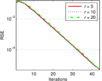
where ϵ1=max{UkVkTLkF,Lk+SkDF,Y1k(V^k)(U^kT)(Y2k)TF}subscriptitalic-ϵ1subscriptnormsubscript𝑈𝑘subscriptsuperscript𝑉𝑇𝑘subscript𝐿𝑘𝐹subscriptnormsubscript𝐿𝑘subscript𝑆𝑘𝐷𝐹subscriptnormsubscriptsuperscript𝑌𝑘1superscriptsubscript^𝑉𝑘superscriptsubscriptsuperscript^𝑈𝑇𝑘superscriptsubscriptsuperscript𝑌𝑘2𝑇𝐹\epsilon_{1}\!=\!\max\{\|U_{k}\!V^{T}_{k}\!-\!L_{k}\|_{F},\|L_{k}\!+\!S_{k}\!-\!D\|_{F},\|Y^{k}_{1}(\widehat{V}_{k})^{\dagger}\!-\!(\widehat{U}^{T}_{k})^{\dagger}(Y^{k}_{2})^{T}\|_{F}\}, ϵ2=max{U^kUkF/UkF,V^kVkF/VkF}subscriptitalic-ϵ2subscriptnormsubscript^𝑈𝑘subscript𝑈𝑘𝐹subscriptnormsubscript𝑈𝑘𝐹subscriptnormsubscript^𝑉𝑘subscript𝑉𝑘𝐹subscriptnormsubscript𝑉𝑘𝐹\epsilon_{2}\!=\!\max\{\|\widehat{U}_{k}\!-\!U_{k}\|_{F}/\|U_{k}\|_{F},\|\widehat{V}_{k}\!-\!V_{k}\|_{F}/\|V_{k}\|_{F}\}, (V^k)superscriptsubscript^𝑉𝑘(\widehat{V}_{k})^{\dagger} is the pseudo-inverse of V^ksubscript^𝑉𝑘\widehat{V}_{k}, and ε𝜀\varepsilon is the stopping tolerance. In this paper, we set the stopping tolerance to ϵ=105italic-ϵsuperscript105\epsilon\!=\!10^{-5} for synthetic data and ϵ=104italic-ϵsuperscript104\epsilon\!=\!10^{-4} for real-world problems. As shown in the Supplementary Materials, the stopping tolerance and relative squared error (RSE) of our methods decrease fast, and they converge within only a small number of iterations (usually within 50 iterations).
Refer to caption
Refer to caption
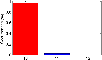
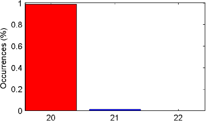
Figure 3: Histograms with the percentage of estimated ranks for Gaussian noise and outlier corrupted matrices of size 500×500500500500\!\times\!500 (left) and 1,000×1,000100010001,000\!\times\!1,000 (right), whose true ranks are 10 and 20, respectively.
Refer to caption

​​ Refer to caption ​​ Refer to caption ​​ Refer to caption ​​ Refer to caption ​​ Refer to caption ​​ Refer to caption
 

Refer to caption
(a) RPCA [44]
Refer to caption
(b) PSVT [45]
Refer to caption
(c) WNNM [46]
Refer to caption
(d) Unifying [49]
Refer to caption
(e) LpSq [31]
Refer to caption
(f) (S+L)1/2subscriptS+L12(\textup{S+L})_{1/2}
Refer to caption
(g) (S+L)2/3subscriptS+L23(\textup{S+L})_{2/3}

​​  ​​  ​​  ​​  ​​  ​​  ​​

Figure 4: Phase transition plots for different algorithms on corrupted matrices of size 200×200200200200\!\times\!200 (top) and 500×500500500500\!\times\!500 (bottom). X-axis denotes the matrix rank, and Y-axis indicates the corruption ratio. The color magnitude indicates the success ratio [0,1]01[0,1], and a larger red area means a better performance of the algorithm (best viewed in colors).

5.3 Computational Complexity

The per-iteration cost of existing Schatten quasi-norm minimization methods such as LpSq [31] is dominated by the computation of the thin SVD of an m×n𝑚𝑛m\!\times\!n matrix with mn𝑚𝑛m\!\geq\!n, and is 𝒪(mn2)𝒪𝑚superscript𝑛2\mathcal{O}(mn^{2}). In contrast, the time complexity of computing SVD for (23) and (24) is 𝒪(md2+nd2)𝒪𝑚superscript𝑑2𝑛superscript𝑑2\mathcal{O}(md^{2}\!+\!nd^{2}). The dominant cost of each iteration in Algorithm 1 corresponds to the matrix multiplications in the update of U𝑈U, V𝑉V and L𝐿L, which take 𝒪(mnd+d3)𝒪𝑚𝑛𝑑superscript𝑑3\mathcal{O}(mnd\!+\!d^{3}). Given that dm,nmuch-less-than𝑑𝑚𝑛d\!\ll\!m,n, the overall complexity of Algorithm 1, as well as Algorithm 2, is thus 𝒪(mnd)𝒪𝑚𝑛𝑑\mathcal{O}(mnd), which is the same as the complexity of LMaFit [47], RegL1 [16], ROSL [64], Unifying [49], and factEN [15].

6 Experimental Results

In this section, we evaluate both the effectiveness and efficiency of our methods (i.e., (S+L)1/2subscriptS+L12(\textup{S+L})_{1/2} and (S+L)2/3subscriptS+L23(\textup{S+L})_{2/3}) for solving extensive synthetic and real-world problems. We also compare our methods with several state-of-the-art methods, such as LMaFit333http://lmafit.blogs.rice.edu/​ [47], RegL1444https://sites.google.com/site/yinqiangzheng/​ [16], Unifying [49], factEN555http://cpslab.snu.ac.kr/people/eunwoo-kim​ [15], RPCA666http://www.cis.pku.edu.cn/faculty/vision/zlin/zlin.htm​ [44], PSVT777http://thohkaistackr.wix.com/page​ [45], WNNM888http://www4.comp.polyu.edu.hk/~cslzhang/​ [46], and LpSq999https://sites.google.com/site/feipingnie/​ [31].

6.1 Rank Estimation

As suggested in [6, 28], the regularization parameter λ𝜆\lambda of our two methods is generally set to max(m,n)𝑚𝑛\sqrt{\max(m,n)}. Analogous to other matrix factorization methods [15, 16, 47, 49], two proposed methods also have another important rank parameter, d𝑑d. To estimate it, we design a simple rank estimation procedure. Since the observed data may be corrupted by noise/outlier and/or missing data, our rank estimation procedure combines two key techniques. First, we efficiently compute the k𝑘k largest singular values of the input matrix (usually k=100𝑘100k\!=\!100), and then use the basic spectral gap technique for determining the number of clusters [78]. Moreover, the rank estimator for incomplete matrices is exploited to look for an index for which the ratio between two consecutive singular values is minimized, as suggested in [79]. We conduct some experiments on corrupted matrices to test the performance of our rank estimation procedure, as shown in Fig. 14. Note that the input matrices are corrupted by both sparse outliers and Gaussian noise as shown below, where the fraction of sparse outliers varies from 00 to 25%percent2525\%, and the noise factor of Gaussian noise is changed from 00 to 0.50.50.5. It can be seen that our rank estimation procedure performs well in terms of robustness to noise and outliers.

TABLE III: Comparison of average RSE, F-M and time (seconds) on corrupted matrices. We highlight the best results in bold and the second best in italic for each of three performance metrics. Note that WNNM and LpSq could not yield experimental results on the largest problem within 24 hours.
RPCA [44] PSVT [45] WNNM [46] Unifying [49] LpSq [31] (S+L)1/2subscriptS+L12(\textup{S+L})_{1/2} (S+L)2/3subscriptS+L23(\textup{S+L})_{2/3}
 m=n𝑚𝑛\!\!\!\!m\!=\!n\!\!\! RSE F-M Time RSE F-M Time RSE F-M Time RSE F-M Time RSE F-M Time RSE F-M Time RSE F-M Time
 ​​500 0.1265 0.8145 6.87 0.1157 0.8298 2.46 0.0581 0.8419 30.59 0.0570 0.8427 1.96 0.1173 0.8213 245.81 0.0469 0.8469 1.70 0.0453 0.8474 1.35
 ​​1,000 0.1138 0.8240 35.29 0.1107 0.8325 16.91 0.0448 0.8461 203.52 0.0443 0.8462 6.93 0.1107 0.8305 985.69 0.0335 0.8495 6.65 0.0318 0.8498 5.89
 ​​5,000 0.1029 0.8324 1,772.55 0.0980 0.8349 1,425.25 0.0315 0.8483 24,370.85 0.0313 0.8488 171.28 0.0152 0.8520 134.15 0.0145 0.8521 128.11
 ​​10,000 0.1002 0.8340 20,321.36 0.0969 0.8355 1,5437.60 0.0302 0.8489 657.41 0.0109 0.8524 528.80 0.0104 0.8525 487.46

6.2 Synthetic Data

We generated the low-rank matrix Lm×nsuperscript𝐿superscript𝑚𝑛L^{*}\!\in\!\mathbb{R}^{m\times n} of rank r𝑟r as the product PQT𝑃superscript𝑄𝑇PQ^{T}, where Pm×r𝑃superscript𝑚𝑟P\!\in\!\mathbb{R}^{m\times r} and Qn×r𝑄superscript𝑛𝑟Q\!\in\!\mathbb{R}^{n\times r} are independent matrices whose elements are independent and identically distributed (i.i.d.) random variables sampled from standard Gaussian distributions. The sparse matrix Sm×nsuperscript𝑆superscript𝑚𝑛S^{*}\!\in\!\mathbb{R}^{m\times n} is generated by the following procedure: its support is chosen uniformly at random and the non-zero entries are i.i.d. random variables sampled uniformly in the interval [5,5]55[-5,5]. The input matrix is D=L+S+N𝐷superscript𝐿superscript𝑆𝑁D\!=\!L^{*}\!+\!S^{*}\!+\!N, where the Gaussian noise is N=nf×𝐫𝐚𝐧𝐝𝐧𝑁𝑛𝑓𝐫𝐚𝐧𝐝𝐧N\!=\!nf\!\times\!\mathbf{randn} and nf0𝑛𝑓0nf\!\geq\!0 is the noise factor. For quantitative evaluation, we measured the performance of low-rank component recovery by the RSE, and evaluated the accuracy of outlier detection by the F-measure (abbreviated to F-M) as in [17]. The higher F-M or lower RSE, the better is the quality of the recovered results.
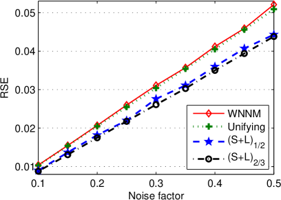
Refer to caption
Refer to caption
Figure 5: Comparison of RSE results on corrupted matrices of size 500×500500500500\!\times\!500 (left) and 1,000×1,000100010001,000\!\times\!1,000 (right) with different noise factors.

6.2.1 Model Comparison

We first compared our methods with RPCA (nuclear norm & 1subscript1\ell_{1}-norm), PSVT (truncated nuclear norm & 1subscript1\ell_{1}-norm), WNNM (weighted nuclear norm & 1subscript1\ell_{1}-norm), LpSq (Schatten q𝑞q-norm & psubscript𝑝\ell_{p}-norm), and Unifying (bilinear spectral penalty & 1subscript1\ell_{1}-norm), where p𝑝p and q𝑞q in LpSq are chosen from the range of {0.1,0.2,,1}0.10.21\{0.1,0.2,\ldots,1\}. A phase transition plot uses magnitude to depict how likely a certain kind of low-rank matrices can be recovered by those methods for a range of different matrix ranks and corruption ratios. If the recovered matrix L𝐿L has a RSE smaller than 102superscript10210^{-2}, we consider the estimation of both L𝐿L and S𝑆S is regarded as successful. Fig. 15 shows the phase transition results of RPCA, PSVT, WNNM, LpSq, Unifying and both our methods on outlier corrupted matrices of size 200×200200200200\times 200 and 500×500500500500\times 500, where the corruption ratios varied from 0 to 0.35 with increment 0.05, and the true rank r𝑟r from 5 to 50 with increment 5. Note that the rank parameter of PSVT, Unifying, and both our methods is set to d=1.25r𝑑1.25𝑟d\!=\!\lfloor 1.25r\rfloor as suggested in [34, 47]. The results show that both our methods perform significantly better than the other methods, which justifies the effectiveness of the proposed RPCA models (15) and (16).

To verify the robustness of our methods, the observed matrices are corrupted by both Gaussian noise and outliers, where the noise factor and outlier ratio are set to nf=0.5𝑛𝑓0.5nf\!=\!0.5 and 20%percent2020\%. The average results (including RSE, F-M, and running time) of 10 independent runs on corrupted matrices with different sizes are reported in Table III. Note that the rank parameter d𝑑d of PSVT, Unifying, and both our methods is computed by our rank estimation procedure. It is clear that both our methods significantly outperform all the other methods in terms of both RSE and F-M in all settings. Those non-convex methods including PSVT, WNNM, LpSq, Unifying, and both our methods consistently perform better than the convex method, RPCA, in terms of both RSE and F-M. Impressively, both our methods are much faster than the other methods, and at least 10 times faster than RPCA, PSVT, WNNM, and LpSq in the case when the size of matrices exceeds 5,000×5,000500050005,000\!\times\!5,000. This actually shows that our methods are more scalable, and have even greater advantage over existing methods for handling large matrices.

We also report the RSE results of both our methods on corrupted matrices of size 500×500500500500\!\times\!500 and 1,000×1,000100010001,000\!\times\!1,000 with outlier ratio 15%, as shown in Fig. 17, where the true ranks of those matrices are 101010 and 202020, and the noise factor ranges from 0.10.10.1 to 0.50.50.5. In addition, we provide the best results of two baseline methods, WNNM and Unifying. Note that the parameter d𝑑d of Unifying and both our methods is computed via our rank estimation procedure. From the results, we can observe that both our methods are much more robust against Gaussian noise than WNNM and Unifying, and have much greater advantage over them in cases when the noise level is relatively large, e.g., 0.50.50.5.

Refer to caption
(a) F-measure vs. outlier ratio
Refer to caption
(b) RSE vs. outlier ratio
Refer to caption
(c) RSE vs. high missing ratio
Refer to caption
(d) RSE vs. low missing ratio
Figure 6: Comparison of different methods on corrupted matrices under varying outlier and missing ratios in terms of RSE and F-measure.
Refer to caption
Refer to caption
Figure 7: Comparison of RSE (left) and F-measure (right) of different methods on corrupted matrices of size 1000×1000100010001000\!\times\!1000 vs. running time.
Refer to caption

​​ Refer to caption ​​ Refer to caption ​​ Refer to caption ​​ Refer to caption ​​ Refer to caption ​​ Refer to caption ​​ Refer to caption

Refer to caption
(a) Images
Refer to caption
(b) RPCA [44]
Refer to caption
(c) PSVT [45]
Refer to caption
(d) WNNM [46]
Refer to caption
(e) Unifying [49]
Refer to caption
(f) LpSq [31]
Refer to caption
(g) (S+L)1/2subscriptS+L12(\textup{S+L})_{1/2}
Refer to caption
(h) (S+L)2/3subscriptS+L23(\textup{S+L})_{2/3}

​​  ​​  ​​  ​​  ​​  ​​  ​​

Figure 8: Text removal results of different methods: detected text masks (top) and recovered background images (bottom). (a) Input image (top) and original image (bottom); (b) RPCA (F-M: 0.9543, RSE: 0.1051); (c) PSVT (F-M: 0.9560, RSE: 0.1007); (d) WNNM (F-M: 0.9536, RSE: 0.0943); (e) Unifying (F-M: 0.9584, RSE: 0.0976); (f) LpSq (F-M: 0.9665, RSE: 0.1097); (g) (S+L)1/2subscriptS+L12(\textup{S+L})_{1/2} (F-M: 0.9905, RSE: 0.0396); and (h) (S+L)2/3subscriptS+L23(\textup{S+L})_{2/3} (F-M: 0.9872, RSE: 0.0463).

6.2.2 Comparisons with Other Methods

Figs. 6(a) and 6(b) show the average F-measure and RSE results of different matrix factorization based methods on 1,000×1,000100010001,000\!\times\!1,000 matrices with different outliers ratios, where the noise factor is set to 0.20.20.2. For fair comparison, the rank parameter of all these methods is set to d=1.25r𝑑1.25𝑟d\!=\!\lfloor 1.25r\rfloor as in [34, 47]. In all cases, RegL1 [16], Unifying [49], factEN [15], and both our methods have significantly better performance than LMaFit [47], where the latter has no regularizers. This empirically verifies the importance of low-rank regularizers including our defined bilinear factor matrix norm penalties. Moreover, we report the average RSE results of these matrix factorization based methods with outlier ratio 5%percent55\% and various missing ratios in Figs. 6(c) and 6(d), in which we also present the results of LpSq. One can see that only with a very limited number of observations (e.g., 80%percent8080\% missing ratio), both our methods yield much more accurate solutions than the other methods including LpSq, while more observations are available, both LpSq and our methods significantly outperform the other methods in terms of RSE.

Finally, we report the performance of all those methods mentioned above on corrupted matrices of size 1000×1000100010001000\!\times\!1000 as running time goes by, as shown in Fig. 18. It is clear that both our methods obtain significantly more accurate solutions than the other methods with much shorter running time. Different from all other methods, the performance of LMaFit becomes even worse over time, which may be caused by the intrinsic model without a regularizer. This also empirically verifies the importance of all low-rank regularizers, including our defined bilinear factor matrix norm penalties, for recovering low-rank matrices.
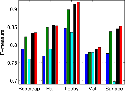
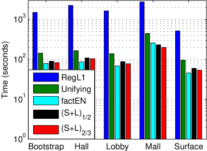
Refer to caption
Refer to caption
Refer to caption
Refer to caption
Refer to caption
Refer to caption
Refer to caption
(a) ​Input, ​segmentation
Refer to caption
(b) RegL1 [16]
Refer to caption
(c) Unifying [49]
Refer to caption
(d) factEN [15]
Refer to caption
(e) (S+L)1/2subscriptS+L12(\textup{S+L})_{1/2}
Refer to caption
(f) (S+L)2/3subscriptS+L23(\textup{S+L})_{2/3}
Figure 9: Background and foreground separation results of different algorithms on the Bootstrap data set. The one frame with missing data of each sequence (top) and its manual segmentation (bottom) are shown in (a). The results of different algorithms are presented from (b) to (f), respectively. The top panel is the recovered background, and the bottom panel is the segmentation.
Refer to caption
Refer to caption
Figure 10: Quantitative comparison for different methods in terms of F-measure (left) and running time (right, in seconds and in logarithmic scale) on five subsequences of surveillance videos.

6.3 Real-world Applications

In this subsection, we apply our methods to solve various low-level vision problems, e.g., text removal, moving object detection, and image alignment and inpainting.

6.3.1 Text Removal

We first apply our methods to detect some text and remove them from the image used in [70]. The ground-truth image is of size 256×256256256256\!\times\!256 with rank equal to 10, as shown in Fig. 8(a). The input data are generated by setting 5% of the randomly selected pixels as missing entries. For fairness, we set the rank parameter of PSVT [45], Unifying [49] and our methods to 202020, and the stopping tolerance ϵ=104italic-ϵsuperscript104\epsilon\!=\!10^{-4} for all these algorithms. The text detection and removal results are shown in Fig. 8, where the text detection accuracy (F-M) and the RSE of recovered low-rank component are also reported. The results show that both our methods significantly outperform the other methods not only visually but also quantitatively. The running time of our methods and the Schatten quasi-norm minimization method, LpSq [31], is 1.36sec, 1.21sec and 77.65sec, respectively, which show that both our methods are more than 50 times faster than LpSq.

6.3.2 Moving Object Detection

We test our methods on real surveillance videos for moving object detection and background subtraction as a RPCA plus matrix completion problem. Background modeling is a crucial task for motion segmentation in surveillance videos. A video sequence satisfies the low-rank and sparse structures, because the background of all the frames is controlled by few factors and hence exhibits low-rank property, and the foreground is detected by identifying spatially localized sparse residuals [6, 17, 40]. We test our methods on real surveillance videos for object detection and background subtraction on five surveillance videos: Bootstrap, Hall, Lobby, Mall and WaterSurface databases101010http://perception.i2r.a-star.edu.sg/. The input data are generated by setting 10% of the randomly selected pixels of each frame as missing entries, as shown in Fig. 9(a).

Figs. 9(b)-9(f) show the foreground and background separation results on the Bootstrap data set. We can see that the background can be effectively extracted by RegL1, Unifying, factEN and both our methods, where their rank parameter is computed via our rank estimation procedure. It is clear that the decomposition results of both our methods are significantly better than that of RegL1 and factEN visually in terms of both background components and foreground segmentation. In addition, we also provide the running time and F-measure of different algorithms on all the five data sets, as shown in Fig. 10, from which we can observe that both our methods consistently outperform the other methods in terms of F-measure. Moreover, Unifying and our methods are much faster than RegL1. Although factEN is slightly faster than Unifying and our methods, it usually has poorer quality of the results.

Refer to caption
Refer to caption
Refer to caption
Refer to caption
Refer to caption
Refer to caption
Refer to caption
Refer to caption
Refer to caption
Refer to caption
Refer to caption
Refer to caption
Refer to caption
Refer to caption
Refer to caption
Refer to caption
Figure 11: Alignment results on the Windows data set used in [50]. The first row: the results generated by RASL [50] (left) and PSVT [45] (right); The second row: the results generated by our (S+L)1/2subscriptS+L12(\textup{S+L})_{1/2} (left) and (S+L)2/3subscriptS+L23(\textup{S+L})_{2/3} (right) methods, respectively. (a) and (e): Aligned images; (b) and (f): Sparse occlusions; (c) and (g): Low-rank components; (d) and (h): Close-up (see red box in the left).

6.3.3 Image Alignment

We also study the performance of our methods in the application of robust image alignment: Given n𝑛n images {I1,,In}subscript𝐼1subscript𝐼𝑛\{I_{1},\ldots,I_{n}\} of an object of interest, the image alignment task aims to align them using a fixed geometric transformation model, such as affine [50]. For this problem, we search for a transformation τ={τ1,,τn}𝜏subscript𝜏1subscript𝜏𝑛\tau\!=\!\{\tau_{1},\ldots,\tau_{n}\} and write Dτ=[vec(I1τ1)||vec(Inτn)]m×n𝐷𝜏delimited-[]vecsubscript𝐼1subscript𝜏1vecsubscript𝐼𝑛subscript𝜏𝑛superscript𝑚𝑛D\!\circ\!\tau\!=\![\textup{vec}(I_{1}\!\circ\!\tau_{1})|\cdots|\textup{vec}(I_{n}\!\circ\!\tau_{n})]\!\in\!\mathbb{R}^{m\times n}. In order to robustly align the set of linearly correlated images despite sparse outliers, we consider the following double nuclear norm regularized model

minU,V,S,τλ2(U+V)+S1/21/2,s.t.,Dτ=UVT+S.subscript𝑈𝑉𝑆𝜏𝜆2subscriptnorm𝑈subscriptnorm𝑉subscriptsuperscriptnorm𝑆12subscript12s.t.𝐷𝜏𝑈superscript𝑉𝑇𝑆\min_{U,V,S,\tau}\frac{\lambda}{2}(\|U\|_{*}\!+\!\|V\|_{*}\!)\!+\!\|S\|^{{1}/{2}}_{\ell_{1/2}},\;\textup{s.t.},D\!\circ\!\tau\!=\!UV^{T}\!+\!S. (34)

Alternatively, our Frobenius/nuclear norm penalty can also be used to address the image alignment problem above.

We first test both our methods on the Windows data set (which contains 16 images of a building, taken from various viewpoints by a perspective camera, and with occlusions due to tree branches) used in [50] and report the aligned results of RASL111111http://perception.csl.illinois.edu/matrix-rank/ [50], PSVT [45] and our methods in Fig. 11, from which it is clear that, compared with RASL and PSVT, both our methods not only robustly align the images, correctly detect and remove the occlusion, but also achieve much better performance in terms of low-rank components, as shown in Figs. 11 and 11, which give the close-up views of the red boxes in Figs. 11 and 11, respectively.

6.3.4 Image Inpainting

Finally, we applied the defined D-N and F-N penalties to image inpainting. As shown by Hu et al. [38]121212https://sites.google.com/site/zjuyaohu/, the images of natural scenes can be viewed as approximately low rank matrices. Naturally, we consider the following D-N penalty regularized least squares problem:

minU,V,Lλ2(U+V)+12𝒫Ω(LD)F2,s.t.,L=UVT.subscript𝑈𝑉𝐿𝜆2subscriptnorm𝑈subscriptnorm𝑉12subscriptsuperscriptnormsubscript𝒫Ω𝐿𝐷2𝐹s.t.𝐿𝑈superscript𝑉𝑇\min_{U,V,L}\!\frac{\lambda}{2}(\|U\|_{*}\!+\!\|V\|_{*}\!)\!+\!\frac{1}{2}\|\mathcal{P}_{\Omega}(L\!-\!D)\|^{2}_{F},\;\textup{s.t.},L\!=\!U\!V^{T}. (35)

The F-N penalty regularized model and the corresponding ADMM algorithms for solving both models are provided in the Supplementary Materials. We compared our methods with one nuclear norm solver [43], one weighted nuclear norm method [37, 46], two truncated nuclear norm methods [38, 45], and one Schatten-q𝑞q quasi-norm method [19]131313As suggested in [19], we chose the qsubscript𝑞\ell_{q}-norm penalty, where q𝑞q was chosen from the range of {0.1,0.2,,1}0.10.21\{0.1,0.2,\ldots,1\}.. Since both of the ADMM algorithms in [38, 45] have very similar performance as shown in [45], we only report the results of [38]. For fair comparison, we set the same values to the parameters d𝑑d, ρ𝜌\rho and μ0subscript𝜇0\mu_{0} for both our methods and [38, 45], e.g., d=9𝑑9d\!=\!9 as in [38].

Fig. 12 shows the 8 test images and some quantitative results (including average PSNR and running time) of all those methods with 85% random missing pixels. We also show the inpainting results of different methods for random mask of 80% missing pixels in Fig. 13 (see the Supplementary Materials for more results with different missing ratios and rank parameters). The results show that both our methods consistently produce much better PSNR results than the other methods in all the settings. As analyzed in [34, 70], our D-N and F-N penalties not only lead to two scalable optimization problems, but also require significantly fewer observations than traditional nuclear norm solvers, e.g., [43]. Moreover, both our methods are much faster than the other methods, in particular, more than 25 times faster than the methods [19, 38, 46].

Refer to caption

Refer to captionRefer to captionRefer to captionRefer to captionRefer to captionRefer to captionRefer to caption

Refer to caption
Figure 12: The natural images used in image inpainting [38] (top), and quantitative comparison of inpainting results (bottom).
Refer to caption
(a) Ground truth
Refer to caption
(b) Input image
Refer to caption
(c) APGL [43] (PSNR: 26.63 dB)
Refer to caption
(d) TNNR [38] (PSNR: 27.47 dB)
Refer to caption
(e) WNNM [46] (PSNR: 27.95 dB)
Refer to caption
(f) IRNN [19] (PSNR: 26.86 dB)
Refer to caption
(g) D-N (PSNR: 28.79 dB)
Refer to caption
(h) F-N (PSNR: 28.64 dB)
Figure 13: Image inpainting results of different methods on Image 7 with 80% random missing pixels (best viewed in colors).

7 Conclusions and Discussions

In this paper we defined the double nuclear norm and Frobenius/nuclear hybrid norm penalties, which are in essence the Schatten-1/2121/2 and 2/3232/3 quasi-norms, respectively. To take advantage of the hyper-Laplacian priors of sparse noise/outliers and singular values of low-rank components, we proposed two novel tractable bilinear factor matrix norm penalized methods for low-level vision problems. Our experimental results show that both our methods can yield more accurate solutions than original Schatten quasi-norm minimization when the number of observations is very limited, while the solutions obtained by the three methods are almost identical when a sufficient number of observations is observed. The effectiveness and generality of both our methods are demonstrated through extensive experiments on both synthetic data and real-world applications, whose results also show that both our methods perform more robust to outliers and missing ratios than existing methods.

An interesting direction of future work is the theoretical analysis of the properties of both of our bilinear factor matrix norm penalties compared to the nuclear norm and the Schatten quasi-norm. For example, how many observations are sufficient for both our models to reliably recover low-rank matrices, although in our experiments we found that our methods perform much better than existing Schatten quasi-norm methods with a limited number of observations. In addition, we are interested in exploring ways to regularize our models with auxiliary information, such as graph Laplacian [27, 80, 81] and hyper-Laplacian matrix [82], or the elastic-net [15]. We can apply our bilinear factor matrix norm penalties to various structured sparse and low-rank problems [5, 17, 28, 33], e.g., corrupted columns [9] and Hankel matrix for image restoration [25].

Acknowledgments

Fanhua Shang, James Cheng and Yuanyuan Liu were supported in part by Grants (CUHK 14206715 & 14222816) from the Hong Kong RGC, ITF 6904079, Grant 3132821 funded by the Research Committee of CUHK. Zhi-Quan Luo was supported in part by the National Science Foundation (NSF) under Grant CCF-1526434, the National Natural Science Foundation of China under Grants 61571384 and 61731018, and the Leading Talents of Guang Dong Province program, Grant No. 00201510. Zhouchen Lin was supported by National Basic Research Program of China (973 Program) (grant no. 2015CB352502), National Natural Science Foundation (NSF) of China (grant nos. 61625301, 61731018, and 61231002), and Qualcomm. Fanhua Shang and Yuanyuan Liu are the corresponding authors.

References

  • [1] M. Aharon, M. Elad, and A. Bruckstein, “K-SVD: An algorithm for designing overcomplete dictionaries for sparse representation,” IEEE Trans. Signal Proces., vol. 54, no. 11, pp. 4311–4322, Nov. 2006.
  • [2] J. Wright, A. Yang, A. Ganesh, S. Sastry, and Y. Ma, “Robust face recognition via sparse representation,” IEEE Trans. Pattern Anal. Mach. Intell., vol. 31, no. 2, pp. 210–227, Feb. 2009.
  • [3] F. De la Torre and M. J. Black, “A framework for robust subspace learning,” Int. J. Comput. Vis., vol. 54, no. 1, pp. 117–142, 2003.
  • [4] E. Elhamifar and R. Vidal, “Sparse subspace clustering: Algorithm, theory, and applications,” IEEE Trans. Pattern Anal. Mach. Intell., vol. 35, no. 11, pp. 2765–2781, Nov. 2013.
  • [5] G. Liu, Z. Lin, S. Yan, J. Sun, Y. Yu, and Y. Ma, “Robust recovery of subspace structures by low-rank representation,” IEEE Trans. Pattern Anal. Mach. Intell., vol. 35, no. 1, pp. 171–184, Jan. 2013.
  • [6] E. J. Candès, X. Li, Y. Ma, and J. Wright, “Robust principal component analysis?” J. ACM, vol. 58, no. 3, pp. 1–37, 2011.
  • [7] M. Tao and X. Yuan, “Recovering low-rank and sparse components of matrices from incomplete and noisy observations,” SIAM J. Optim., vol. 21, no. 1, pp. 57–81, 2011.
  • [8] T. Zhou and D. Tao, “GoDec: Randomized low-rank & sparse matrix decomposition in noisy case,” in Proc. 28th Int. Conf. Mach. Learn., 2011, pp. 33–40.
  • [9] Y. Chen, H. Xu, C. Caramanis, and S. Sanghavi, “Robust matrix completion with corrupted columns,” in Proc. 28th Int. Conf. Mach. Learn., 2011, pp. 873–880.
  • [10] D. Krishnan and R. Fergus, “Fast image deconvolution using hyper-Laplacian priors,” in Proc. Adv. Neural Inf. Process. Syst., 2009, pp. 1033–1041.
  • [11] S. Mallat, “A theory for multiresolution signal decomposition: The wavelet representation,” IEEE Trans. Pattern Anal. Mach. Intell., vol. 11, no. 7, pp. 674–693, Jul. 1989.
  • [12] L. Luo, J. Yang, J. Qian, and Y. Tai, “Nuclear-L1subscript𝐿1{L}_{1} norm joint regression for face reconstruction and recognition with mixed noise,” Pattern Recogn., vol. 48, no. 12, pp. 3811–3824, 2015.
  • [13] A. Eriksson and A. van den Hengel, “Efficient computation of robust low-rank matrix approximations in the presence of missing data using the L1subscript𝐿1{L}_{1} norm,” in Proc. IEEE Conf. Comput. Vis. Pattern Recognit., 2010, pp. 771–778.
  • [14] Q. Ke and T. Kanade, “Robust L1subscript𝐿1{L}_{1} norm factorization in the presence of outliers and missing data by alternative convex programming,” in Proc. IEEE Conf. Comput. Vis. Pattern Recognit., 2005, pp. 739–746.
  • [15] E. Kim, M. Lee, and S. Oh, “Elastic-net regularization of singular values for robust subspace learning,” in Proc. IEEE Conf. Comput. Vis. Pattern Recognit., 2015, pp. 915–923.
  • [16] Y. Zheng, G. Liu, S. Sugimoto, S. Yan, and M. Okutomi, “Practical low-rank matrix approximation under robust L1subscript𝐿1{L}_{1}-norm,” in Proc. IEEE Conf. Comput. Vis. Pattern Recognit., 2012, pp. 1410–1417.
  • [17] X. Zhou, C. Yang, and W. Yu, “Moving object detection by detecting contiguous outliers in the low-rank representation,” IEEE Trans. Pattern Anal. Mach. Intell., vol. 35, no. 3, pp. 597–610, Mar. 2013.
  • [18] J. Fan and R. Li, “Variable selection via nonconcave penalized likelihood and its Oracle properties,” J. Am. Statist. Assoc., vol. 96, no. 456, pp. 1348–1360, 2001.
  • [19] C. Lu, J. Tang, S. Yan, and Z. Lin, “Generalized nonconvex nonsmooth low-rank minimization,” in Proc. IEEE Conf. Comput. Vis. Pattern Recognit., 2014, pp. 4130–4137.
  • [20] C. Zhang, “Nearly unbiased variable selection under minimax concave penalty,” Ann. Statist., vol. 38, no. 2, pp. 894–942, 2010.
  • [21] Z. Xu, X. Chang, F. Xu, and H. Zhang, “L1/2subscript𝐿12{L}_{1/2} regularization: A thresholding representation theory and a fast solver,” IEEE Trans. Neural Netw. Learn. Syst., vol. 23, no. 7, pp. 1013–1027, Jul. 2012.
  • [22] W. Zuo, D. Meng, L. Zhang, X. Feng, and D. Zhang, “A generalized iterated shrinkage algorithm for non-convex sparse coding,” in Proc. IEEE Int. Conf. Comput. Vis., 2013, pp. 217–224.
  • [23] J. Cai, E. J. Candès, and Z. Shen, “A singular value thresholding algorithm for matrix completion,” SIAM J. Optim., vol. 20, no. 4, pp. 1956–1982, 2010.
  • [24] V. Chandrasekaran, S. Sanghavi, P. Parrilo, and A. Willsky, “Rank-sparsity incoherence for matrix decomposition,” SIAM J. Optim., vol. 21, no. 2, pp. 572–596, 2011.
  • [25] K. Jin and J. Ye, “Annihilating filter-based low-rank Hankel matrix approach for image inpainting,” IEEE Trans. Image Process., vol. 24, no. 11, pp. 3498–3511, Nov. 2015.
  • [26] B. Recht, M. Fazel, and P. Parrilo, “Guaranteed minimum-rank solutions of linear matrix equations via nuclear norm minimization,” SIAM Rev., vol. 52, no. 3, pp. 471–501, 2010.
  • [27] N. Shahid, V. Kalofolias, X. Bresson, M. Bronstein, and P. Vandergheynst, “Robust principal component analysis on graphs,” in Proc. IEEE Int. Conf. Comput. Vis., 2015, pp. 2812–2820.
  • [28] H. Zhang, Z. Lin, C. Zhang, and E. Chang, “Exact recoverability of robust PCA via outlier pursuit with tight recovery bounds,” in Proc. 29th AAAI Conf. Artif. Intell., 2015, pp. 3143–3149.
  • [29] Z. Zhang, A. Ganesh, X. Liang, and Y. Ma, “TILT: Transform invariant low-rank textures,” Int. J. Comput. Vis., vol. 99, no. 1, pp. 1–24, 2012.
  • [30] Z. Gu, M. Shao, L. Li, and Y. Fu, “Discriminative metric: Schatten norm vs. vector norm,” in Proc. 21st Int. Conf. Pattern Recog., 2012, pp. 1213–1216.
  • [31] F. Nie, H. Wang, X. Cai, H. Huang, and C. Ding, “Robust matrix completion via joint Schatten p𝑝p-norm and Lpsubscript𝐿𝑝{L}_{p}-norm minimization,” in Proc. IEEE Int. Conf. Data Mining, 2012, pp. 566–574.
  • [32] M. Lai, Y. Xu, and W. Yin, “Improved iteratively rewighted least squares for unconstrained smoothed psubscript𝑝\ell_{p} minimization,” SIAM J. Numer. Anal., vol. 51, no. 2, pp. 927–957, 2013.
  • [33] C. Lu, Z. Lin, and S. Yan, “Smoothed low rank and sparse matrix recovery by iteratively reweighted least squares minimization,” IEEE Trans. Image Process., vol. 24, no. 2, pp. 646–654, Feb. 2015.
  • [34] F. Shang, Y. Liu, and J. Cheng, “Scalable algorithms for tractable Schatten quasi-norm minimization,” in Proc. 30th AAAI Conf. Artif. Intell., 2016, pp. 2016–2022.
  • [35] G. H. Golub and C. F. V. Loan, Matrix Computations, Fourth ed.   Johns Hopkins University Press, 2013.
  • [36] S. Wang, L. Zhang, and Y. Liang, “Nonlocal spectral prior model for low-level vision,” in Proc. Asian Conf. Comput. Vis., 2013, pp. 231–244.
  • [37] S. Gu, L. Zhang, W. Zuo, and X. Feng, “Weighted nuclear norm minimization with application to image denoising,” in Proc. IEEE Conf. Comput. Vis. Pattern Recognit., 2014, pp. 2862–2869.
  • [38] Y. Hu, D. Zhang, J. Ye, X. Li, and X. He, “Fast and accurate matrix completion via truncated nuclear norm regularization,” IEEE Trans. Pattern Anal. Mach. Intell., vol. 35, no. 9, pp. 2117–2130, Sep. 2013.
  • [39] W. Bian, X. Chen, and Y. Ye, “Complexity analysis of interior point algorithms for non-Lipschitz and nonconvex minimization,” Math. Program., vol. 149, no. 1, pp. 301–327, 2015.
  • [40] J. Wright, A. Ganesh, S. Rao, Y. Peng, and Y. Ma, “Robust principal component analysis: exact recovery of corrupted low-rank matrices by convex optimization,” in Proc. Adv. Neural Inf. Process. Syst., 2009, pp. 2080–2088.
  • [41] J. Wright, A. Ganesh, K. Min, and Y. Ma, “Compressive principal component pursuit,” Inform. Infer., vol. 2, no. 1, pp. 32–68, 2013.
  • [42] F. Shang, Y. Liu, H. Tong, J. Cheng, and H. Cheng, “Robust bilinear factorization with missing and grossly corrupted observations,” Inform. Sciences, vol. 307, pp. 53–72, 2015.
  • [43] K.-C. Toh and S. Yun, “An accelerated proximal gradient algorithm for nuclear norm regularized least squares problems,” Pac. J. Optim., vol. 6, pp. 615–640, 2010.
  • [44] Z. Lin, M. Chen, and L. Wu, “The augmented Lagrange multiplier method for exact recovery of corrupted low-rank matrices,” Univ. Illinois, Urbana-Champaign, Tech. Rep., Mar. 2009.
  • [45] T. Oh, Y. Tai, J. Bazin, H. Kim, and I. Kweon, “Partial sum minimization of singular values in robust PCA: Algorithm and applications,” IEEE Trans. Pattern Anal. Mach. Intell., vol. 38, no. 4, pp. 744–758, Apr. 2016.
  • [46] S. Gu, Q. Xie, D. Meng, W. Zuo, X. Feng, and L. Zhang, “Weighted nuclear norm minimization and its applications to low level vision,” Int. J. Comput. Vis., vol. 121, no. 2, pp. 183–208, 2017.
  • [47] Y. Shen, Z. Wen, and Y. Zhang, “Augmented Lagrangian alternating direction method for matrix separation based on low-rank factorization,” Optim. Method Softw., vol. 29, no. 2, pp. 239–263, 2014.
  • [48] Y. Liu, L. Jiao, and F. Shang, “A fast tri-factorization method for low-rank matrix recovery and completion,” Pattern Recogn., vol. 46, no. 1, pp. 163–173, 2013.
  • [49] R. Cabral, F. De la Torre, J. Costeira, and A. Bernardino, “Unifying nuclear norm and bilinear factorization approaches for low-rank matrix decomposition,” in Proc. IEEE Int. Conf. Comput. Vis., 2013, pp. 2488–2495.
  • [50] Y. Peng, A. Ganesh, J. Wright, W. Xu, and Y. Ma, “RASL: Robust alignment by sparse and low-rank decomposition for linearly correlated images,” IEEE Trans. Pattern Anal. Mach. Intell., vol. 34, no. 11, pp. 2233–2246, Nov. 2012.
  • [51] H. Ji, C. Liu, Z. Shen, and Y. Xu, “Robust video denoising using low rank matrix completion,” in Proc. IEEE Conf. Comput. Vis. Pattern Recognit., 2010, pp. 1791–1798.
  • [52] D. L. Donoho, “De-noising by soft-thresholding,” IEEE Trans. Inform. Theory, vol. 41, no. 3, pp. 613–627, May 1995.
  • [53] H. Xu, C. Caramanis, and S. Sanghavi, “Robust PCA via outlier pursuit,” in Proc. Adv. Neural Inf. Process. Syst., 2010, pp. 2496–2504.
  • [54] Y. Yang, Z. Ma, A. G. Hauptmann, and N. Sebe, “Feature selection for multimedia analysis by sharing information among multiple tasks,” IEEE Trans. Multimedia, vol. 15, no. 3, pp. 661–669, Apr. 2013.
  • [55] Z. Ma, Y. Yang, N. Sebe, and A. G. Hauptmann, “Knowledge adaptation with partially shared features for event detection using few exemplars,” IEEE Trans. Pattern Anal. Mach. Intell., vol. 36, no. 9, pp. 1789–1802, Sep. 2014.
  • [56] M. Shao, D. Kit, and Y. Fu, “Generalized transfer subspace learning through low-rank constraint,” Int. J. Comput. Vis., vol. 109, no. 1, pp. 74–93, 2014.
  • [57] Z. Ding, M. Shao, and S. Yan, “Missing modality transfer learning via latent low-rank constraint,” IEEE Trans. Image Process., vol. 24, no. 11, pp. 4322–4334, Nov. 2015.
  • [58] S. Boyd, N. Parikh, E. Chu, B. Peleato, and J. Eckstein, “Distributed optimization and statistical learning via the alternating direction method of multipliers,” Found. Trends Mach. Learn., vol. 3, no. 1, pp. 1–122, 2011.
  • [59] T. Oh, Y. Matsushita, Y. Tai, and I. Kweon, “Fast randomized singular value thresholding for nuclear norm minimization,” in Proc. IEEE Conf. Comput. Vis. Pattern Recognit., 2015, pp. 4484–4493.
  • [60] R. Larsen, “PROPACK-software for large and sparse SVD calculations,” 2005.
  • [61] J. Cai and S. Osher, “Fast singular value thresholding without singular value decomposition,” Methods Anal. appl., vol. 20, no. 4, pp. 335–352, 2013.
  • [62] F. J. amd M. Oskarsson and K. Åstrom, “On the minimal problems of low-rank matrix factorization,” in Proc. IEEE Conf. Comput. Vis. Pattern Recognit., 2015, pp. 2549–2557.
  • [63] S. Xiao, W. Li, D. Xu, and D. Tao, “FaLRR: A fast low rank representation solver,” in Proc. IEEE Int. Conf. Comput. Vis., 2015, pp. 4612–4620.
  • [64] X. Shu, F. Porikli, and N. Ahuja, “Robust orthonormal subspace learning: Efficient recovery of corrupted low-rank matrices,” in Proc. IEEE Conf. Comput. Vis. Pattern Recognit., 2014, pp. 3874–3881.
  • [65] F. Shang, Y. Liu, J. Cheng, and H. Cheng, “Robust principal component analysis with missing data,” in Proc. 23rd ACM Int. Conf. Inf. Knowl. Manag., 2014, pp. 1149–1158.
  • [66] G. Liu and S. Yan, “Active subspace: Toward scalable low-rank learning,” Neur. Comp., vol. 24, no. 12, pp. 3371–3394, 2012.
  • [67] N. Srebro, J. Rennie, and T. Jaakkola, “Maximum-margin matrix factorization,” in Proc. Adv. Neural Inf. Process. Syst., 2004, pp. 1329–1336.
  • [68] J. Feng, H. Xu, and S. Yan, “Online robust PCA via stochastic optimization,” in Proc. Adv. Neural Inf. Process. Syst., 2013, pp. 404–412.
  • [69] R. Sun and Z.-Q. Luo, “Guaranteed matrix completion via non-convex factorization,” IEEE Trans. Inform. Theory, vol. 62, no. 11, pp. 6535–6579, Nov. 2016.
  • [70] F. Shang, Y. Liu, and J. Cheng, “Tractable and scalable Schatten quasi-norm approximations for rank minimization,” in Proc. 19th Int. Conf. Artif. Intell. Statist., 2016, pp. 620–629.
  • [71] L. Mirsky, “A trace inequality of John von Neumann,” Monatsh. Math., vol. 79, pp. 303–306, 1975.
  • [72] J. von Neumann, “Some matrix-inequalities and metrization of matric-space,” Tomsk Univ. Rev., vol. 1, pp. 286–300, 1937.
  • [73] R. Mazumder, T. Hastie, and R. Tibshirani, “Spectral regularization algorithms for learning large incomplete matrices,” J. Mach. Learn. Res., vol. 11, pp. 2287–2322, 2010.
  • [74] W. Cao, J. Sun, and Z. Xu, “Fast image deconvolution using closed-form thresholding formulas of lqsubscript𝑙𝑞l_{q} (q=12,23𝑞1223q\!=\!\frac{1}{2},\frac{2}{3}) regularization,” J. Vis. Commun. Image R., vol. 24, no. 1, pp. 31–41, 2013.
  • [75] J. Bolte, S. Sabach, and M. Teboulle, “Proximal alternating linearized minimization for nonconvex and nonsmooth problems,” Math. Program., vol. 146, no. 1, pp. 459–494, 2014.
  • [76] M. Hong, Z.-Q. Luo, and M. Razaviyayn, “Convergence analysis of alternating direction method of multipliers for a family of nonconvex problems,” SIAM J. Optim., vol. 26, no. 1, pp. 337–364, 2016.
  • [77] C. Chen, B. He, Y. Ye, and X. Yuan, “The direct extension of ADMM for multi-block convex minimization problems is not necessarily convergent,” Math. Program., vol. 155, no. 1-2, pp. 57–79, 2016.
  • [78] U. von Luxburg, “A tutorial on spectral clustering,” Stat. Comput., vol. 17, no. 4, pp. 395–416, 2007.
  • [79] R. Keshavan, A. Montanari, and S. Oh, “Low-rank matrix completion with noisy observations: a quantitative comparison,” in 47th Conf. Commun. Control Comput., 2009, pp. 1216–1222.
  • [80] Y. Yang, D. Xu, F. Nie, S. Yan, and Y. Zhuang, “Image clustering using local discriminant models and global integration,” IEEE Trans. Image Process., vol. 19, no. 10, pp. 2761–2773, Oct. 2010.
  • [81] Y. Yang, F. Nie, D. Xu, J. Luo, Y. Zhuang, and Y. Pan, “A multimedia retrieval framework based on semi-supervised ranking and relevance feedback,” IEEE Trans. Pattern Anal. Mach. Intell., vol. 34, no. 4, pp. 723–742, Apr. 2012.
  • [82] M. Yin, J. Gao, and Z. Lin, “Laplacian regularized low-rank representation and its applications,” IEEE Trans. Pattern Anal. Mach. Intell., vol. 38, no. 3, pp. 504–517, Mar. 2016.
  • [83] I. Daubechies, M. Defrise, and C. De Mol, “An iterative thresholding algorithm for linear inverse problems with a sparsity constraint,” Commun. Pur. Appl. Math., vol. 57, no. 11, pp. 1413–1457, 2004.
  • [84] E. T. Hale, W. Yin, and Y. Zhang, “Fixed-point continuation for 1subscript1\ell_{1}-minimization: Methodology and convergence,” SIAM J. Optim., vol. 19, no. 3, pp. 1107–1130, 2008.
  • [85] F. Wang, W. Cao, and Z. Xu, “Convergence of multi-block Bregman ADMM for nonconvex composite problems,” arXiv:1505.03063, 2015.
[Uncaptioned image] Fanhua Shang (M’14) received the Ph.D. degree in Circuits and Systems from Xidian University, Xi’an, China, in 2012. He is currently a Research Associate with the Department of Computer Science and Engineering, The Chinese University of Hong Kong. From 2013 to 2015, he was a Post-Doctoral Research Fellow with the Department of Computer Science and Engineering, The Chinese University of Hong Kong. From 2012 to 2013, he was a Post-Doctoral Research Associate with the Department of Electrical and Computer Engineering, Duke University, Durham, NC, USA. His current research interests include machine learning, data mining, pattern recognition, and computer vision.
[Uncaptioned image] James Cheng is an Assistant Professor with the Department of Computer Science and Engineering, The Chinese University of Hong Kong, Hong Kong. His current research interests include distributed computing systems, large-scale network analysis, temporal networks, and big data.
[Uncaptioned image] Yuanyuan Liu received the Ph.D. degree in Pattern Recognition and Intelligent System from Xidian University, Xi’an, China, in 2013. She is currently a Post-Doctoral Research Fellow with the Department of Computer Science and Engineering, The Chinese University of Hong Kong. Prior to that, she was a Post-Doctoral Research Fellow with the Department of Systems Engineering and Engineering Management, CUHK. Her current research interests include image processing, pattern recognition, and machine learning.
[Uncaptioned image] Zhi-Quan (Tom) Luo (F’07) received the B.Sc. degree in Applied Mathematics in 1984 from Peking University, Beijing, China. Subsequently, he was selected by a joint committee of the American Mathematical Society and the Society of Industrial and Applied Mathematics to pursue Ph.D. study in the USA. He received the Ph.D. degree in operations research in 1989 from the Operations Research Center and the Department of Electrical Engineering and Computer Science, MIT, Cambridge, MA, USA. From 1989 to 2003, Dr. Luo held a faculty position with the Department of Electrical and Computer Engineering, McMaster University, Hamilton, Canada, where he eventually became the department head and held a Canada Research Chair in Information Processing. Since April of 2003, he has been with the Department of Electrical and Computer Engineering at the University of Minnesota (Twin Cities) as a full professor. His research interests lies in the union of optimization algorithms, signal processing and digital communication. Currently, he is with the Chinese University of Hong Kong, Shenzhen, where he is a Professor and serves as the Vice President Academic. Dr. Luo is a fellow of SIAM. He is a recipient of the 2004, 2009 and 2011 IEEE Signal Processing Society Best Paper Awards, the 2011 EURASIP Best Paper Award and the 2011 ICC Best Paper Award. He was awarded the 2010 Farkas Prize from the INFRMS Optimization Society. Dr. Luo chaired the IEEE Signal Processing Society Technical Committee on the Signal Processing for Communications (SPCOM) from 2011-2012. He has held editorial positions for several international journals including Journal of Optimization Theory and Applications, SIAM Journal on Optimization, Mathematics of Computation and IEEE TRANSACTIONS ON SIGNAL PROCESSING. In 2014 he is elected to the Royal Society of Canada.
[Uncaptioned image] Zhouchen Lin (M’00-SM’08) received the PhD degree in applied mathematics from Peking University in 2000. He is currently a professor with the Key Laboratory of Machine Perception, School of Electronics Engineering and Computer Science, Peking University. His research interests include computer vision, image processing, machine learning, pattern recognition, and numerical optimization. He is an area chair of CVPR 2014/2016, ICCV 2015, and NIPS 2015, and a senior program committee member of AAAI 2016/2017/2018 and IJCAI 2016. He is an associate editor of the IEEE Transactions on Pattern Analysis and Machine Intelligence and the International Journal of Computer Vision. He is an IAPR Fellow.

Supplementary Materials:
Bilinear Factor Matrix Norm Minimization for Robust PCA: Algorithms and Applications

Fanhua Shang,  James Cheng, Yuanyuan Liu, Zhi-Quan Luo,  and Zhouchen Lin,  F. Shang, J. Cheng and Y. Liu are with the Department of Computer Science and Engineering, The Chinese University of Hong Kong, Shatin, N.T., Hong Kong. E-mail: {fhshang, jcheng, yyliu}@cse.cuhk.edu.hk.Z.-Q. Luo is with Shenzhen Research Institute of Big Data, the Chinese University of Hong Kong, Shenzhen, China and Department of Electrical and Computer Engineering, University of Minnesota, Minneapolis, MN 55455, USA. E-mail: luozq@cuhk.edu.cn and luozq@umn.edu.Z. Lin is with Key Laboratory of Machine Perception (MOE), School of EECS, Peking University, Beijing 100871, P.R. China, and the Cooperative Medianet Innovation Center, Shanghai Jiao Tong University, Shanghai 200240, P.R. China. E-mail: zlin@pku.edu.cn.

Supplementary Materials:

Bilinear Factor Matrix Norm Minimization for Robust PCA: Algorithms and Applications

In this supplementary material, we give the detailed proofs of some theorems, lemmas and properties. We also provide the stopping criterion of our algorithms and the details of Algorithm 2. In addition, we present two new ADMM algorithms for image recovery application and their pseudo-codes, and some additional experimental results for both synthetic and real-world datasets.

Notations

lsuperscript𝑙\mathbb{R}^{l} denotes the l𝑙l-dimensional Euclidean space, and the set of all m×n𝑚𝑛m\!\times\!n matrices141414Without loss of generality, we assume mn𝑚𝑛m\!\geq\!n in this paper. with real entries is denoted by m×nsuperscript𝑚𝑛\mathbb{R}^{m\times n}. Tr(XTY)=ijXijYijTrsuperscript𝑋𝑇𝑌subscript𝑖𝑗subscript𝑋𝑖𝑗subscript𝑌𝑖𝑗\textrm{Tr}(X^{T}Y)=\sum_{ij}X_{ij}Y_{ij}, where Tr()Tr\textrm{Tr}(\cdot) denotes the trace of a matrix. We assume the singular values of Xm×n𝑋superscript𝑚𝑛X\!\in\!\mathbb{R}^{m\times n} are ordered as σ1(X)σ2(X)σr(X)>σr+1(X)==σn(X)=0subscript𝜎1𝑋subscript𝜎2𝑋subscript𝜎𝑟𝑋subscript𝜎𝑟1𝑋subscript𝜎𝑛𝑋0\sigma_{1}(X)\geq\sigma_{2}(X)\geq\cdots\geq\sigma_{r}(X)>\sigma_{r+1}(X)=\cdots=\sigma_{n}(X)=0, where r=rank(X)𝑟rank𝑋r=\textrm{rank}(X). Then the SVD of X𝑋X is denoted by X=UΣVT𝑋𝑈Σsuperscript𝑉𝑇X=U\Sigma V^{T}, where Σ=diag(σ1,,σn)Σdiagsubscript𝜎1subscript𝜎𝑛\Sigma=\textrm{diag}(\sigma_{1},\ldots,\sigma_{n}). Insubscript𝐼𝑛I_{n} denotes an identity matrix of size n×n𝑛𝑛n\!\times\!n.

Definition 5.

For any vector xl𝑥superscript𝑙x\in\mathbb{R}^{l}, its psubscript𝑝\ell_{p}-norm for 0<p<0𝑝0\!<\!p\!<\!\infty is defined as

xp=(i=1l|xi|p)1/psubscriptnorm𝑥subscript𝑝superscriptsubscriptsuperscript𝑙𝑖1superscriptsubscript𝑥𝑖𝑝1𝑝\|x\|_{\ell_{p}}=\left(\sum^{l}_{i=1}|x_{i}|^{p}\right)^{1/p}

where xisubscript𝑥𝑖x_{i} is the i𝑖i-th element of x𝑥x. When p=1𝑝1p\!=\!1, the 1subscript1\ell_{1}-norm of x𝑥x is x1=i|xi|subscriptnorm𝑥subscript1subscript𝑖subscript𝑥𝑖\|x\|_{\ell_{1}}\!=\!\sum_{i}|x_{i}| (which is convex), while the psubscript𝑝\ell_{p}-norm of x𝑥x is a quasi-norm when 0<p<10𝑝10\!<\!p\!<\!1, which is non-convex and violates the triangle inequality. In addition, the 2subscript2\ell_{2}-norm of x𝑥x is x2=ixi2subscriptnorm𝑥subscript2subscript𝑖subscriptsuperscript𝑥2𝑖\|x\|_{\ell_{2}}\!=\!\sqrt{\sum_{i}x^{2}_{i}}.

The above definition can be naturally extended from vectors to matrices by the following form

Sp=(i,j|Sij|p)1/p.subscriptnorm𝑆subscript𝑝superscriptsubscript𝑖𝑗superscriptsubscript𝑆𝑖𝑗𝑝1𝑝\|S\|_{\ell_{p}}=\left(\sum_{i,j}|S_{ij}|^{p}\right)^{1/p}.
Definition 6.

The Schatten-p𝑝p norm (0<p<0𝑝0\!<\!p\!<\!\infty) of a matrix Xm×n𝑋superscript𝑚𝑛X\!\in\!\mathbb{R}^{m\times n} is defined as follows:

XSp=(i=1nσip(X))1/psubscriptnorm𝑋subscript𝑆𝑝superscriptsubscriptsuperscript𝑛𝑖1subscriptsuperscript𝜎𝑝𝑖𝑋1𝑝\|X\|_{S_{p}}=\left(\sum^{n}_{i=1}\sigma^{p}_{i}(X)\right)^{1/p}

where σi(X)subscript𝜎𝑖𝑋\sigma_{i}(X) denotes the i𝑖i-th largest singular value of X𝑋X.

In the following, we will list some special cases of the Schatten-p𝑝p norm (0<p<0𝑝0\!<\!p\!<\!\infty).

  • When 0<p<10𝑝10\!<\!p\!<\!1, the Schatten-p𝑝p norm is a quasi-norm, and it is non-convex and violates the triangle inequality.

  • When p=1𝑝1p\!=\!1, the Schatten-1 norm (also known as the nuclear norm or trace norm) of X𝑋X is defined as

    X=i=1nσi(X).subscriptnorm𝑋subscriptsuperscript𝑛𝑖1subscript𝜎𝑖𝑋\|X\|_{\ast}=\sum^{n}_{i=1}\sigma_{i}(X).
  • When p=2𝑝2p\!=\!2, the Schatten-2 norm is more commonly called the Frobenius norm151515Note that the Frobenius norm is the induced norm of the 2subscript2\ell_{2}-norm on matrices. defined as

    XF=i=1nσi2(X)=i,jXij2.subscriptnorm𝑋𝐹subscriptsuperscript𝑛𝑖1subscriptsuperscript𝜎2𝑖𝑋subscript𝑖𝑗subscriptsuperscript𝑋2𝑖𝑗\|X\|_{F}=\sqrt{\sum^{n}_{i=1}\sigma^{2}_{i}(X)}=\sqrt{\sum_{i,j}X^{2}_{ij}}.

APPENDIX A: Proof of Lemma 2

To prove Lemma 2, we first define the doubly stochastic matrix, and give the following lemma.

Definition 7.

A square matrix is doubly stochastic if its elements are non-negative real numbers, and the sum of elements of each row or column is equal to 111.

Lemma 7.

Let Pn×n𝑃superscript𝑛𝑛P\!\in\!\mathbb{R}^{n\times n} be a doubly stochastic matrix, and if

0x1x2xn,y1y2yn0,formulae-sequence0subscript𝑥1subscript𝑥2subscript𝑥𝑛subscript𝑦1subscript𝑦2subscript𝑦𝑛0\!\!0\leq x_{1}\leq x_{2}\leq\ldots\leq x_{n},\;y_{1}\geq y_{2}\geq\ldots\geq y_{n}\geq 0, (36)

then

i,j=1npijxiyjk=1nxkyk.subscriptsuperscript𝑛𝑖𝑗1subscript𝑝𝑖𝑗subscript𝑥𝑖subscript𝑦𝑗subscriptsuperscript𝑛𝑘1subscript𝑥𝑘subscript𝑦𝑘\sum^{n}_{i,j=1}p_{ij}x_{i}y_{j}\geq\sum^{n}_{k=1}x_{k}y_{k}.

The proof of Lemma 7 is essentially similar to that of the lemma in [71], thus we give the following proof sketch for this lemma.

Proof:

Using (36), there exist non-negative numbers αisubscript𝛼𝑖\alpha_{i} and βjsubscript𝛽𝑗\beta_{j} for all 1i,jnformulae-sequence1𝑖𝑗𝑛1\leq i,j\leq n such that

xk=1ikαi,yk=kjnβjfor allk=1,,n.formulae-sequenceformulae-sequencesubscript𝑥𝑘subscript1𝑖𝑘subscript𝛼𝑖subscript𝑦𝑘subscript𝑘𝑗𝑛subscript𝛽𝑗for all𝑘1𝑛x_{k}=\sum_{1\leq i\leq k}\alpha_{i},\;\;y_{k}=\sum_{k\leq j\leq n}\beta_{j}\,\;\textup{for all}\;\,k=1,\ldots,n.

Let δijsubscript𝛿𝑖𝑗\delta_{ij} denote the Kronecker delta (i.e., δij=1subscript𝛿𝑖𝑗1\delta_{ij}\!=\!1 if i=j𝑖𝑗i\!=\!j, and δij=0subscript𝛿𝑖𝑗0\delta_{ij}\!=\!0 otherwise), we have

k=1nxkyki,j=1npijxiyj=i,j=1n(δijpij)xiyj=1i,jn(δijpij)1riαrjsnβs=1r,snαrβsrin,1js(δijpij).subscriptsuperscript𝑛𝑘1subscript𝑥𝑘subscript𝑦𝑘subscriptsuperscript𝑛𝑖𝑗1subscript𝑝𝑖𝑗subscript𝑥𝑖subscript𝑦𝑗subscriptsuperscript𝑛𝑖𝑗1subscript𝛿𝑖𝑗subscript𝑝𝑖𝑗subscript𝑥𝑖subscript𝑦𝑗subscriptformulae-sequence1𝑖𝑗𝑛subscript𝛿𝑖𝑗subscript𝑝𝑖𝑗subscript1𝑟𝑖subscript𝛼𝑟subscript𝑗𝑠𝑛subscript𝛽𝑠subscriptformulae-sequence1𝑟𝑠𝑛subscript𝛼𝑟subscript𝛽𝑠subscriptformulae-sequence𝑟𝑖𝑛1𝑗𝑠subscript𝛿𝑖𝑗subscript𝑝𝑖𝑗\begin{split}&\sum^{n}_{k=1}x_{k}y_{k}-\sum^{n}_{i,j=1}p_{ij}x_{i}y_{j}=\sum^{n}_{i,j=1}(\delta_{ij}-p_{ij})x_{i}y_{j}\\ =&\sum_{1\leq i,j\leq n}(\delta_{ij}-p_{ij})\sum_{1\leq r\leq i}\!\alpha_{r}\sum_{j\leq s\leq n}\!\beta_{s}\\ =&\sum_{1\leq r,s\leq n}\alpha_{r}\beta_{s}\sum_{r\leq i\leq n,1\leq j\leq s}(\delta_{ij}-p_{ij}).\end{split}

If rs𝑟𝑠r\leq s, by the lemma in [71] we know that

1i<r,1js(δijpij)0,andsubscriptformulae-sequence1𝑖𝑟1𝑗𝑠subscript𝛿𝑖𝑗subscript𝑝𝑖𝑗0and\begin{split}\sum_{1\leq i<r,1\leq j\leq s}(\delta_{ij}-p_{ij})\geq 0,\;\;\textup{and}\end{split}
rin,1js(δijpij)+1i<r,1js(δijpij)=0.subscriptformulae-sequence𝑟𝑖𝑛1𝑗𝑠subscript𝛿𝑖𝑗subscript𝑝𝑖𝑗subscriptformulae-sequence1𝑖𝑟1𝑗𝑠subscript𝛿𝑖𝑗subscript𝑝𝑖𝑗0\sum_{r\leq i\leq n,1\leq j\leq s}(\delta_{ij}-p_{ij})+\sum_{1\leq i<r,1\leq j\leq s}(\delta_{ij}-p_{ij})=0.

Therefore, we have

rin,1js(δijpij)0.subscriptformulae-sequence𝑟𝑖𝑛1𝑗𝑠subscript𝛿𝑖𝑗subscript𝑝𝑖𝑗0\sum_{r\leq i\leq n,1\leq j\leq s}(\delta_{ij}-p_{ij})\leq 0.

The same result can be obtained in a similar way for rs𝑟𝑠r\!\geq\!s. ∎

Proof of Lemma 2:

Proof:

Using the properties of the trace, we know that

Tr(XTY)=i,j=1n(UX)ij2λiτj.Trsuperscript𝑋𝑇𝑌subscriptsuperscript𝑛𝑖𝑗1subscriptsuperscriptsubscript𝑈𝑋2𝑖𝑗subscript𝜆𝑖subscript𝜏𝑗\textrm{Tr}(X^{T}Y)=\sum^{n}_{i,j=1}(U_{X})^{2}_{ij}\lambda_{i}\tau_{j}.

Note that UXsubscript𝑈𝑋U_{X} is a unitary matrix, i.e., UXTUX=UXUXT=Insubscriptsuperscript𝑈𝑇𝑋subscript𝑈𝑋subscript𝑈𝑋subscriptsuperscript𝑈𝑇𝑋subscript𝐼𝑛U^{T}_{X}U_{X}\!=\!U_{X}U^{T}_{X}\!=\!I_{n}, which implies that ((UX)ij2)subscriptsuperscriptsubscript𝑈𝑋2𝑖𝑗((U_{X})^{2}_{ij}) is a doubly stochastic matrix. By Lemma 7, we have Tr(XTY)i=1nλiτiTrsuperscript𝑋𝑇𝑌subscriptsuperscript𝑛𝑖1subscript𝜆𝑖subscript𝜏𝑖\textrm{Tr}(X^{T}Y)\geq\sum^{n}_{i=1}\lambda_{i}\tau_{i}. ∎

APPENDIX B: Proofs of Theorems 1 and 2

Proof of Theorem 1:

Proof:

Using Lemma 3, for any factor matrices Um×d𝑈superscript𝑚𝑑U\!\in\!\mathbb{R}^{m\times d} and Vn×d𝑉superscript𝑛𝑑V\!\in\!\mathbb{R}^{n\times d} with the constraint X=UVT𝑋𝑈superscript𝑉𝑇X\!=\!UV^{T}, we have

(U+V2)2XS1/2.superscriptsubscriptnorm𝑈subscriptnorm𝑉22subscriptnorm𝑋subscript𝑆12\left(\frac{\|U\|_{\ast}+\|V\|_{\ast}}{2}\right)^{2}\geq\|X\|_{S_{1/2}}.

On the other hand, let U=LXΣX1/2superscript𝑈subscript𝐿𝑋subscriptsuperscriptΣ12𝑋U^{\star}\!=\!L_{X}\Sigma^{1/2}_{X} and V=RXΣX1/2superscript𝑉subscript𝑅𝑋subscriptsuperscriptΣ12𝑋V^{\star}\!=\!R_{X}\Sigma^{1/2}_{X}, where X=LXΣXRXT𝑋subscript𝐿𝑋subscriptΣ𝑋subscriptsuperscript𝑅𝑇𝑋X\!=\!L_{X}\Sigma_{X}R^{T}_{X} is the SVD of X𝑋X as in Lemma 3, then we have

X=U(V)TandXS1/2=(U+V)2/4.𝑋superscript𝑈superscriptsuperscript𝑉𝑇andsubscriptnorm𝑋subscript𝑆12superscriptsubscriptnormsuperscript𝑈subscriptnormsuperscript𝑉24X=U^{\star}(V^{\star})^{T}\;\;\textup{and}\;\;\|X\|_{S_{1/2}}=(\|U^{\star}\|_{\ast}+\|V^{\star}\|_{\ast})^{2}/4.

Therefore, we have

minU,V:X=UVT(U+V2)2=XS1/2.\min_{U,V:X=UV^{T}}\!\left(\frac{\|U\|_{\ast}+\|V\|_{\ast}}{2}\right)^{2}=\|X\|_{S_{1/2}}.

This completes the proof. ∎

Proof of Theorem 2:

Proof:

Using Lemma 4, for any Um×d𝑈superscript𝑚𝑑U\!\in\!\mathbb{R}^{m\times d} and Vn×d𝑉superscript𝑛𝑑V\!\in\!\mathbb{R}^{n\times d} with the constraint X=UVT𝑋𝑈superscript𝑉𝑇X\!=\!UV^{T}, we have

(UF2+2V3)3/2XS2/3.superscriptsubscriptsuperscriptnorm𝑈2𝐹2subscriptnorm𝑉332subscriptnorm𝑋subscript𝑆23\left(\frac{\|U\|^{2}_{F}+2\|V\|_{\ast}}{3}\right)^{3/2}\geq\|X\|_{S_{2/3}}.

On the other hand, let U=LXΣX1/3superscript𝑈subscript𝐿𝑋subscriptsuperscriptΣ13𝑋U^{\star}\!=\!L_{X}\Sigma^{1/3}_{X} and V=RXΣX2/3superscript𝑉subscript𝑅𝑋subscriptsuperscriptΣ23𝑋V^{\star}\!=\!R_{X}\Sigma^{2/3}_{X}, where X=LXΣXRXT𝑋subscript𝐿𝑋subscriptΣ𝑋subscriptsuperscript𝑅𝑇𝑋X\!=\!L_{X}\Sigma_{X}R^{T}_{X} is the SVD of X𝑋X as in Lemma 3, then we have

X=U(V)TandXS2/3=[(UF2+2V)/3]3/2.𝑋superscript𝑈superscriptsuperscript𝑉𝑇andsubscriptnorm𝑋subscript𝑆23superscriptdelimited-[]subscriptsuperscriptnormsuperscript𝑈2𝐹2subscriptnormsuperscript𝑉332X=U^{\star}(V^{\star})^{T}\;\;\textup{and}\;\;\|X\|_{S_{2/3}}=[(\|U^{\star}\|^{2}_{F}+2\|V^{\star}\|_{\ast})/3]^{3/2}.

Thus, we have

minU,V:X=UVT(UF2+2V3)3/2=XS2/3.\min_{U,V:X=UV^{T}}\!\left(\frac{\|U\|^{2}_{F}+2\|V\|_{\ast}}{3}\right)^{3/2}=\|X\|_{S_{2/3}}.

This completes the proof. ∎

APPENDIX C: Proof of Property 4

Proof:

The proof of Property 4 involves some properties of the psubscript𝑝\ell_{p}-norm, which we recall as follows. For any vector x𝑥x in nsuperscript𝑛\mathbb{R}^{n} and 0<p2p110subscript𝑝2subscript𝑝110<p_{2}\leq p_{1}\leq 1, the following inequalities hold:

x1xp1,xp1xp2n1p21p1xp1.formulae-sequencesubscriptnorm𝑥subscript1subscriptnorm𝑥subscriptsubscript𝑝1subscriptnorm𝑥subscriptsubscript𝑝1subscriptnorm𝑥subscriptsubscript𝑝2superscript𝑛1subscript𝑝21subscript𝑝1subscriptnorm𝑥subscriptsubscript𝑝1\|x\|_{\ell_{1}}\leq\|x\|_{\ell_{p_{1}}},\quad\|x\|_{\ell_{p_{1}}}\leq\|x\|_{\ell_{p_{2}}}\leq n^{\frac{1}{p_{2}}-\frac{1}{p_{1}}}\|x\|_{\ell_{p_{1}}}.

Let X𝑋X be an m×n𝑚𝑛{m\times n} matrix of rank r𝑟r, and denote its compact SVD by X=Um×rΣr×rVn×rT𝑋subscript𝑈𝑚𝑟subscriptΣ𝑟𝑟subscriptsuperscript𝑉𝑇𝑛𝑟X=U_{m\times r}\Sigma_{r\times r}V^{T}_{n\times r}. By Theorems 1 and 2, and the properties of the psubscript𝑝\ell_{p}-norm mentioned above, we have

X=diag(Σr×r)1diag(Σr×r)12=XD-Nrank(X)X,X=diag(Σr×r)1diag(Σr×r)23=XF-Nrank(X)X.formulae-sequencesubscriptdelimited-∥∥𝑋subscriptdelimited-∥∥diagsubscriptΣ𝑟𝑟subscript1subscriptdelimited-∥∥diagsubscriptΣ𝑟𝑟subscript12subscriptdelimited-∥∥𝑋D-Nrank𝑋subscriptdelimited-∥∥𝑋subscriptdelimited-∥∥𝑋subscriptdelimited-∥∥diagsubscriptΣ𝑟𝑟subscript1subscriptdelimited-∥∥diagsubscriptΣ𝑟𝑟subscript23subscriptdelimited-∥∥𝑋F-Nrank𝑋subscriptdelimited-∥∥𝑋\begin{split}\|X\|_{\ast}&=\|\textrm{diag}(\Sigma_{r\times r})\|_{\ell_{1}}\leq\|\textrm{diag}(\Sigma_{r\times r})\|_{\ell_{\frac{1}{2}}}=\|X\|_{\textup{D-N}}\leq\textup{rank}(X)\|X\|_{\ast},\\ \|X\|_{\ast}&=\|\textrm{diag}(\Sigma_{r\times r})\|_{\ell_{1}}\leq\|\textrm{diag}(\Sigma_{r\times r})\|_{\ell_{\frac{2}{3}}}=\|X\|_{\textup{F-N}}\leq\sqrt{\textup{rank}(X)}\|X\|_{\ast}.\end{split}

In addition,

XF-N=diag(Σr×r)23diag(Σr×r)12=XD-N.subscriptnorm𝑋F-NsubscriptnormdiagsubscriptΣ𝑟𝑟subscript23subscriptnormdiagsubscriptΣ𝑟𝑟subscript12subscriptnorm𝑋D-N\|X\|_{\textup{F-N}}=\|\textrm{diag}(\Sigma_{r\times r})\|_{\ell_{\frac{2}{3}}}\leq\|\textrm{diag}(\Sigma_{r\times r})\|_{\ell_{\frac{1}{2}}}=\|X\|_{\textup{D-N}}.

Therefore, we have

XXF-NXD-Nrank(X)X.subscriptnorm𝑋subscriptnorm𝑋F-Nsubscriptnorm𝑋D-Nrank𝑋subscriptnorm𝑋\|X\|_{\ast}\leq\|X\|_{\textup{F-N}}\leq\|X\|_{\textup{D-N}}\leq\textup{rank}(X)\|X\|_{\ast}.

This completes the proof. ∎

Algorithm 2 ADMM for solving (S+L)2/3subscriptS+L23(\textup{S+L})_{2/3} problem (18)
0:  Dm×n𝐷superscript𝑚𝑛D\!\in\!\mathbb{R}^{m\times n}, the given rank d𝑑d and λ𝜆\lambda.
0:  μ0subscript𝜇0\mu_{0}, ρ>1𝜌1\rho\!>\!1, k=0𝑘0k\!=\!0, and ϵitalic-ϵ\epsilon.
1:  while not converged do
2:     while not converged do
3:        Update Uk+1subscript𝑈𝑘1U_{k+1} and Vk+1subscript𝑉𝑘1V_{k+1} by (61) and (62), respectively.
4:        Update V^k+1subscript^𝑉𝑘1\widehat{V}_{k+1} by V^k+1=𝒟2λ/3μk(Vk+1(Y2)k/μk)subscript^𝑉𝑘1subscript𝒟2𝜆3subscript𝜇𝑘subscript𝑉𝑘1subscriptsubscript𝑌2𝑘subscript𝜇𝑘\widehat{V}_{k+1}=\mathcal{D}_{2\lambda/3\mu_{k}}\!\left(V_{k+1}\!-\!(Y_{2})_{k}/\mu_{k}\right).
5:        Update Lk+1subscript𝐿𝑘1L_{k+1} and Sk+1subscript𝑆𝑘1S_{k+1} by (43) and (33) in this paper, respectively.
6:     end while  //monospace-//\verb|//| Inner loop
7:     Update the multipliers Y1k+1subscriptsuperscript𝑌𝑘11Y^{k+\!1}_{1}, Y2k+1subscriptsuperscript𝑌𝑘12Y^{k+\!1}_{2} and Y3k+1subscriptsuperscript𝑌𝑘13Y^{k+\!1}_{3} by Y1k+1=Y1k+μk(V^k+1Vk+1)subscriptsuperscript𝑌𝑘11subscriptsuperscript𝑌𝑘1subscript𝜇𝑘subscript^𝑉𝑘1subscript𝑉𝑘1\quad Y^{k+\!1}_{1}\!=\!Y^{k}_{1}\!+\!\mu_{k}(\widehat{V}_{k+\!1}\!-\!V_{k+\!1}), Y2k+1=Y2k+μk(Uk+1Vk+1TLk+1)subscriptsuperscript𝑌𝑘12subscriptsuperscript𝑌𝑘2subscript𝜇𝑘subscript𝑈𝑘1subscriptsuperscript𝑉𝑇𝑘1subscript𝐿𝑘1Y^{k+\!1}_{2}\!=\!Y^{k}_{2}\!+\!\mu_{k}(U_{k+\!1}V^{T}_{k+\!1}\!-\!L_{k+\!1}), and Y3k+1=Y3k+μk(Lk+1+Sk+1D)subscriptsuperscript𝑌𝑘13subscriptsuperscript𝑌𝑘3subscript𝜇𝑘subscript𝐿𝑘1subscript𝑆𝑘1𝐷Y^{k+\!1}_{3}\!=\!Y^{k}_{3}\!+\!\mu_{k}(L_{k+\!1}\!+\!S_{k+\!1}\!-\!D).
8:     Update μk+1subscript𝜇𝑘1\mu_{k+1} by μk+1=ρμksubscript𝜇𝑘1𝜌subscript𝜇𝑘\mu_{k+1}=\rho\mu_{k}.
9:     kk+1𝑘𝑘1k\leftarrow k+1.
10:  end while  //monospace-//\verb|//| Outer loop
10:  Uk+1subscript𝑈𝑘1U_{k+1} and Vk+1subscript𝑉𝑘1V_{k+1}.

APPENDIX D: Solving (18) via ADMM

Similar to Algorithm 1, we also propose an efficient algorithm based on the alternating direction method of multipliers (ADMM) to solve (18), whose augmented Lagrangian function is given by

μ(U,V,L,S,V^,Y1,Y2,Y3)=λ3(UF2+2V^)+𝒫Ω(S)2/32/3+Y1,V^V+Y2,UVTL+Y3,L+SD+μ2(UVTLF2+V^VF2+L+SDF2)subscript𝜇𝑈𝑉𝐿𝑆^𝑉subscript𝑌1subscript𝑌2subscript𝑌3𝜆3subscriptsuperscriptdelimited-∥∥𝑈2𝐹2subscriptdelimited-∥∥^𝑉subscriptsuperscriptdelimited-∥∥subscript𝒫Ω𝑆23subscript23subscript𝑌1^𝑉𝑉subscript𝑌2𝑈superscript𝑉𝑇𝐿subscript𝑌3𝐿𝑆𝐷𝜇2subscriptsuperscriptdelimited-∥∥𝑈superscript𝑉𝑇𝐿2𝐹subscriptsuperscriptdelimited-∥∥^𝑉𝑉2𝐹subscriptsuperscriptdelimited-∥∥𝐿𝑆𝐷2𝐹\begin{split}\mathcal{L}_{\mu}(U,V,L,S,\widehat{V},Y_{1},Y_{2},Y_{3})=&\,\frac{\lambda}{3}\!\left(\|U\|^{2}_{F}\!+\!2\|\widehat{V}\|_{*}\right)+\|\mathcal{P}_{\Omega}(S)\|^{2/3}_{\ell_{2/3}}\!+\!\left\langle Y_{1},\widehat{V}\!-\!V\right\rangle\!+\!\left\langle Y_{2},UV^{T}\!-\!L\right\rangle\!+\!\left\langle Y_{3},L\!+\!S\!-\!D\right\rangle\\ &+\frac{\mu}{2}\left(\|UV^{T}-L\|^{2}_{F}+\|\widehat{V}-V\|^{2}_{F}+\|L+S-D\|^{2}_{F}\right)\end{split}

where Y1n×dsubscript𝑌1superscript𝑛𝑑Y_{1}\!\in\!\mathbb{R}^{n\times d}, Y2m×nsubscript𝑌2superscript𝑚𝑛Y_{2}\!\in\!\mathbb{R}^{m\times n} and Y3m×nsubscript𝑌3superscript𝑚𝑛Y_{3}\!\in\!\mathbb{R}^{m\times n} are the matrices of Lagrange multipliers.

Update of Uk+1subscript𝑈𝑘1U_{k+1} and Vk+1subscript𝑉𝑘1V_{k+1}:

For updating Uk+1subscript𝑈𝑘1{U}_{k+1} and Vk+1subscript𝑉𝑘1{V}_{k+1}, we consider the following optimization problems:

minUλ3UF2+μk2UVkTLk+μk1Y2kF2,subscript𝑈𝜆3subscriptsuperscriptnorm𝑈2𝐹subscript𝜇𝑘2subscriptsuperscriptnorm𝑈subscriptsuperscript𝑉𝑇𝑘subscript𝐿𝑘subscriptsuperscript𝜇1𝑘subscriptsuperscript𝑌𝑘22𝐹\min_{U}\frac{\lambda}{3}\|U\|^{2}_{F}+\frac{\mu_{k}}{2}\|UV^{T}_{k}-L_{k}+\mu^{-\!1}_{k}Y^{k}_{2}\|^{2}_{F}, (37)
minVV^kV+μk1Y1kF2+Uk+1VTLk+μk1Y2kF2,subscript𝑉subscriptsuperscriptnormsubscript^𝑉𝑘𝑉subscriptsuperscript𝜇1𝑘subscriptsuperscript𝑌𝑘12𝐹subscriptsuperscriptnormsubscript𝑈𝑘1superscript𝑉𝑇subscript𝐿𝑘subscriptsuperscript𝜇1𝑘subscriptsuperscript𝑌𝑘22𝐹\min_{V}\|\widehat{V}_{k}-V+\mu^{-\!1}_{\!k}Y^{k}_{1}\|^{2}_{F}+\|U_{\!k+\!1}V^{T}\!-L_{k}+\mu^{-\!1}_{\!k}Y^{k}_{2}\|^{2}_{F}, (38)

and their optimal solutions can be given by

Uk+1=μkPkVk(2λ3Id+μkVkTVk)1,subscript𝑈𝑘1subscript𝜇𝑘subscript𝑃𝑘subscript𝑉𝑘superscript2𝜆3subscript𝐼𝑑subscript𝜇𝑘subscriptsuperscript𝑉𝑇𝑘subscript𝑉𝑘1U_{k+1}=\mu_{k}P_{k}V_{k}\left(\frac{2\lambda}{3}I_{d}+\mu_{k}V^{T}_{k}V_{k}\right)^{-\!1}, (39)
Vk+1=[V^k+μk1Y1k+PkTUk+1](Id+Uk+1TUk+1)1,subscript𝑉𝑘1delimited-[]subscript^𝑉𝑘subscriptsuperscript𝜇1𝑘subscriptsuperscript𝑌𝑘1subscriptsuperscript𝑃𝑇𝑘subscript𝑈𝑘1superscriptsubscript𝐼𝑑subscriptsuperscript𝑈𝑇𝑘1subscript𝑈𝑘11V_{k+1}=\left[\widehat{V}_{k}+\mu^{-\!1}_{k}Y^{k}_{1}+P^{T}_{k}U_{k+\!1}\right]\left(I_{d}+U^{T}_{k+\!1}U_{k+\!1}\right)^{-\!1}, (40)

where Pk=Lkμk1Y2ksubscript𝑃𝑘subscript𝐿𝑘subscriptsuperscript𝜇1𝑘subscriptsuperscript𝑌𝑘2P_{k}\!=\!L_{k}-\mu^{\!-\!1}_{k}Y^{k}_{2}.

Update of V^k+1subscript^𝑉𝑘1\widehat{V}_{k+1}:

To update V^k+1subscript^𝑉𝑘1\widehat{V}_{k+1}, we fix the other variables and solve the following optimization problem

minV^2λ3V^+μk2V^Vk+1+Y1k/μkF2.subscript^𝑉2𝜆3subscriptnorm^𝑉subscript𝜇𝑘2subscriptsuperscriptnorm^𝑉subscript𝑉𝑘1subscriptsuperscript𝑌𝑘1subscript𝜇𝑘2𝐹\min_{\widehat{V}}\frac{2\lambda}{3}\|\widehat{V}\|_{*}+\frac{\mu_{k}}{2}\|\widehat{V}-V_{k+1}+Y^{k}_{1}/\mu_{k}\|^{2}_{F}. (41)

Similar to (23) and (24), the closed-form solution of (41) can also be obtained by the SVT operator [23] defined as follows.

Definition 8.

Let Y𝑌Y be a matrix of size m×n𝑚𝑛m\!\times\!n (mn𝑚𝑛m\geq n), and UYΣYVYTsubscript𝑈𝑌subscriptΣ𝑌subscriptsuperscript𝑉𝑇𝑌U_{Y}\Sigma_{Y}V^{T}_{Y} be its SVD. Then the singular value thresholding (SVT) operator 𝒟τsubscript𝒟𝜏\mathcal{D}_{\tau} is defined as [23]:

𝒟τ(Y)=UY𝒮τ(ΣY)VYT,subscript𝒟𝜏𝑌subscript𝑈𝑌subscript𝒮𝜏subscriptΣ𝑌subscriptsuperscript𝑉𝑇𝑌\mathcal{D}_{\tau}(Y)=U_{Y}\mathcal{S}_{\tau}(\Sigma_{Y})V^{T}_{Y},

where 𝒮τ(x)=max(|x|τ,0)sgn(x)subscript𝒮𝜏𝑥𝑥𝜏0sgn𝑥\mathcal{S}_{\tau}(x)=\max(|x|-\tau,0)\cdot\textup{sgn}(x) is the soft shrinkage operator [83, 52, 84].

Update of Lk+1subscript𝐿𝑘1L_{k+1}:

For updating Lk+1subscript𝐿𝑘1L_{k+\!1}, we consider the following optimization problem:

minLUk+1Vk+1TL+μk1Y2kF2+L+SkD+μk1Y3kF2.subscript𝐿subscriptsuperscriptnormsubscript𝑈𝑘1subscriptsuperscript𝑉𝑇𝑘1𝐿subscriptsuperscript𝜇1𝑘subscriptsuperscript𝑌𝑘22𝐹subscriptsuperscriptnorm𝐿subscript𝑆𝑘𝐷subscriptsuperscript𝜇1𝑘subscriptsuperscript𝑌𝑘32𝐹\min_{L}\|U_{k+\!1}\!V^{T}_{k+\!1}\!-\!L\!+\!\mu^{\!-\!1}_{k}Y^{k}_{2}\|^{2}_{F}+\|L\!+\!S_{k}\!-\!D\!+\!\mu^{-\!1}_{k}Y^{k}_{3}\|^{2}_{F}. (42)

Since (42) is a least squares problem, and thus its closed-form solution is given by

Lk+1=12(Uk+1Vk+1T+μk1Y2kSk+Dμk1Y3k).subscript𝐿𝑘112subscript𝑈𝑘1subscriptsuperscript𝑉𝑇𝑘1subscriptsuperscript𝜇1𝑘subscriptsuperscript𝑌𝑘2subscript𝑆𝑘𝐷subscriptsuperscript𝜇1𝑘subscriptsuperscript𝑌𝑘3L_{k+\!1}=\frac{1}{2}\!\left(U_{k+\!1}\!V^{T}_{k+\!1}+\mu^{-\!1}_{k}Y^{k}_{2}-S_{k}+D-\mu^{-\!1}_{k}Y^{k}_{3}\right). (43)

Together with the update scheme of Sk+1subscript𝑆𝑘1S_{k+1}, as stated in (33) in this paper, we develop an efficient ADMM algorithm to solve the Frobenius/nuclear hybrid norm penalized RPCA problem (18), as outlined in Algorithm 2

APPENDIX E: Proof of Theorem 3

In this part, we first prove the boundedness of multipliers and some variables of Algorithm 1, and then we analyze the convergence of Algorithm 1. To prove the boundedness, we first give the following lemma.

Lemma 8 ([44]).

Let \mathcal{H} be a real Hilbert space endowed with an inner product ,\langle\cdot,\cdot\rangle and a corresponding norm \|\!\cdot\!\|, and yx𝑦norm𝑥y\!\in\!\partial\|x\|, where f(x)𝑓𝑥\partial f(x) denotes the subgradient of f(x)𝑓𝑥f(x). Then y=1superscriptnorm𝑦1\|y\|^{*}\!=\!1 if x0𝑥0x\neq 0, and y1superscriptnorm𝑦1\|y\|^{*}\!\leq\!1 if x=0𝑥0x\!=\!0, where \|\!\cdot\!\|^{*} is the dual norm of \|\!\cdot\!\|. For instance, the dual norm of the nuclear norm is the spectral norm, 2\|\!\cdot\!\|_{2}, i.e., the largest singular value.

Lemma 9 (Boundedness).

Let Y1k+1=Y1k+μk(U^k+1Uk+1)subscriptsuperscript𝑌𝑘11subscriptsuperscript𝑌𝑘1subscript𝜇𝑘subscript^𝑈𝑘1subscript𝑈𝑘1Y^{k+\!1}_{1}\!=\!Y^{k}_{1}\!+\!\mu_{k}(\widehat{U}_{k+\!1}\!-\!U_{k+\!1}), Y2k+1=Y2k+μk(V^k+1Vk+1)subscriptsuperscript𝑌𝑘12subscriptsuperscript𝑌𝑘2subscript𝜇𝑘subscript^𝑉𝑘1subscript𝑉𝑘1Y^{k+\!1}_{2}\!=\!Y^{k}_{2}\!+\!\mu_{k}(\widehat{V}_{k+\!1}\!-\!V_{k+\!1}), Y3k+1=Y3k+μk(Uk+1Vk+1TLk+1)subscriptsuperscript𝑌𝑘13subscriptsuperscript𝑌𝑘3subscript𝜇𝑘subscript𝑈𝑘1subscriptsuperscript𝑉𝑇𝑘1subscript𝐿𝑘1Y^{k+\!1}_{3}\!=\!Y^{k}_{3}\!+\!\mu_{k}(U_{k+\!1}\!V^{T}_{k+\!1}\!-\!L_{k+\!1}) and Y4k+1=Y4k+μk(Lk+1+Sk+1D)subscriptsuperscript𝑌𝑘14subscriptsuperscript𝑌𝑘4subscript𝜇𝑘subscript𝐿𝑘1subscript𝑆𝑘1𝐷Y^{k+\!1}_{4}\!=\!Y^{k}_{4}\!+\!\mu_{k}(L_{k+\!1}\!+\!S_{k+\!1}\!-\!D). Suppose that μksubscript𝜇𝑘\mu_{k} is non-decreasing and k=0μk+1μk4/3<subscriptsuperscript𝑘0subscript𝜇𝑘1subscriptsuperscript𝜇43𝑘\sum^{\infty}_{k=0}\!\frac{\mu_{k+\!1}}{\mu^{4/3}_{k}}\!<\!\infty, then the sequences {(Uk,Vk)}subscript𝑈𝑘subscript𝑉𝑘\{(U_{k},V_{k})\}, {(U^k,V^k)}subscript^𝑈𝑘subscript^𝑉𝑘\{(\widehat{U}_{k},\widehat{V}_{k})\}, {(Y1k,Y2k,Y4k/μk13)}subscriptsuperscript𝑌𝑘1subscriptsuperscript𝑌𝑘2subscriptsuperscript𝑌𝑘43subscript𝜇𝑘1\{(Y^{k}_{1},Y^{k}_{2},Y^{k}_{4}/\!\sqrt[3]{\mu_{k-\!1}})\}, {Lk}subscript𝐿𝑘\{L_{k}\} and {Sk}subscript𝑆𝑘\{S_{k}\} produced by Algorithm 1 are all bounded.

Proof:

Let 𝒰k:=(Uk,Vk)assignsubscript𝒰𝑘subscript𝑈𝑘subscript𝑉𝑘\mathscr{U}_{k}\!:=\!(U_{k},V_{k}), 𝒱k:=(U^k,V^k)assignsubscript𝒱𝑘subscript^𝑈𝑘subscript^𝑉𝑘\mathscr{V}_{k}\!:=\!(\widehat{U}_{k},\widehat{V}_{k}) and 𝒴k:=(Y1k,Y2k,Y3k,Y4k)assignsubscript𝒴𝑘subscriptsuperscript𝑌𝑘1subscriptsuperscript𝑌𝑘2subscriptsuperscript𝑌𝑘3subscriptsuperscript𝑌𝑘4\mathscr{Y}_{k}\!:=\!(Y^{k}_{1},Y^{k}_{2},Y^{k}_{3},Y^{k}_{4}). By the first-order optimality conditions of the augmented Lagrangian function of (17) with respect to U^^𝑈\widehat{U} and V^^𝑉\widehat{V} (i.e., Problems (23) and (24)), we have

0U^μk(𝒰k+1,𝒱k+1,Lk+1,Sk+1,𝒴k)and  0V^μk(𝒰k+1,𝒱k+1,Lk+1,Sk+1,𝒴k),0subscript^𝑈subscriptsubscript𝜇𝑘subscript𝒰𝑘1subscript𝒱𝑘1subscript𝐿𝑘1subscript𝑆𝑘1subscript𝒴𝑘and  0subscript^𝑉subscriptsubscript𝜇𝑘subscript𝒰𝑘1subscript𝒱𝑘1subscript𝐿𝑘1subscript𝑆𝑘1subscript𝒴𝑘0\in\partial_{\widehat{U}}\mathcal{L}_{\mu_{k}}(\mathscr{U}_{k+1},\mathscr{V}_{k+1},L_{k+1},S_{k+1},\mathscr{Y}_{k})\;\;\textup{and}\;\;0\in\partial_{\widehat{V}}\mathcal{L}_{\mu_{k}}(\mathscr{U}_{k+1},\mathscr{V}_{k+1},L_{k+1},S_{k+1},\mathscr{Y}_{k}),

i.e., Y1k+1λ2U^k+1subscriptsuperscript𝑌𝑘11𝜆2subscriptnormsubscript^𝑈𝑘1-Y^{k+1}_{1}\!\in\!\frac{\lambda}{2}\partial\|\widehat{U}_{k+1}\|_{\ast} and Y2k+1λ2V^k+1subscriptsuperscript𝑌𝑘12𝜆2subscriptnormsubscript^𝑉𝑘1-Y^{k+1}_{2}\!\in\!\frac{\lambda}{2}\partial\|\widehat{V}_{k+1}\|_{\ast}, where Y1k+1=μk(U^k+1Uk+1+Y1k/μk)subscriptsuperscript𝑌𝑘11subscript𝜇𝑘subscript^𝑈𝑘1subscript𝑈𝑘1subscriptsuperscript𝑌𝑘1subscript𝜇𝑘Y^{k+1}_{1}\!=\!\mu_{k}(\widehat{U}_{k+\!1}\!-\!U_{k+\!1}\!+\!Y^{k}_{1}/\mu_{k}) and Y2k+1=μk(V^k+1Vk+1+Y2k/μk)subscriptsuperscript𝑌𝑘12subscript𝜇𝑘subscript^𝑉𝑘1subscript𝑉𝑘1subscriptsuperscript𝑌𝑘2subscript𝜇𝑘Y^{k+1}_{2}\!=\!\mu_{k}(\widehat{V}_{k+\!1}\!-\!V_{k+\!1}\!+\!Y^{k}_{2}/\mu_{k}). By Lemma 8, we obtain

Y1k+12λ2andY2k+12λ2,subscriptnormsubscriptsuperscript𝑌𝑘112𝜆2andsubscriptnormsubscriptsuperscript𝑌𝑘122𝜆2\|Y^{k+1}_{1}\|_{2}\leq\frac{\lambda}{2}\;\;\textup{and}\;\;\|Y^{k+1}_{2}\|_{2}\leq\frac{\lambda}{2},

which implies that the sequences {Y1k}subscriptsuperscript𝑌𝑘1\{Y^{k}_{1}\} and {Y2k}subscriptsuperscript𝑌𝑘2\{Y^{k}_{2}\} are bounded.

Next we prove the boundedness of {Y4k/μk13}subscriptsuperscript𝑌𝑘43subscript𝜇𝑘1\{Y^{k}_{4}\!/\!\sqrt[3]{\mu_{k-1}}\}. Using (27), it is easy to show that 𝒫Ω(Y4k+1)=0subscriptsuperscript𝒫perpendicular-toΩsubscriptsuperscript𝑌𝑘140\mathcal{P}^{\perp}_{\Omega}(Y^{k+1}_{4})\!=\!0, which implies that the sequence {𝒫Ω(Y4k+1)}subscriptsuperscript𝒫perpendicular-toΩsubscriptsuperscript𝑌𝑘14\{\mathcal{P}^{\perp}_{\Omega}(Y^{k+1}_{4})\} is bounded. Let A=DLk+1μk1Y4k𝐴𝐷subscript𝐿𝑘1subscriptsuperscript𝜇1𝑘subscriptsuperscript𝑌𝑘4A\!=\!D\!-\!L_{k+1}\!-\!\mu^{-1}_{k}Y^{k}_{4}, and Φ(S):=𝒫Ω(S)1/21/2assignΦ𝑆subscriptsuperscriptnormsubscript𝒫Ω𝑆12subscript12\Phi(S)\!:=\!\|\mathcal{P}_{\Omega}(S)\|^{1/2}_{\ell_{1/2}}. To prove the boundedness of {Y4k/μk13}subscriptsuperscript𝑌𝑘43subscript𝜇𝑘1\{Y^{k}_{4}\!/\!\sqrt[3]{\mu_{k-1}}\}, we consider the following two cases.

Case 1: |aij|>32μk23,(i,j)Ω.formulae-sequencesubscript𝑎𝑖𝑗323subscriptsuperscript𝜇2𝑘𝑖𝑗Ω|a_{ij}|>\frac{3}{2\sqrt[3]{\mu^{2}_{k}}},\,(i,j)\!\in\!\Omega.

If |aij|>32μk23subscript𝑎𝑖𝑗323subscriptsuperscript𝜇2𝑘|a_{ij}|\!>\!\frac{3}{2\sqrt[3]{\mu^{2}_{k}}}, and using Proposition 1, then |[Sk+1]ij|>0subscriptdelimited-[]subscript𝑆𝑘1𝑖𝑗0|[S_{k+1}]_{ij}|>0. The first-order optimality condition of (27) implies that

[Φ(Sk+1)]ij+[Y4k+1]ij=0,subscriptdelimited-[]Φsubscript𝑆𝑘1𝑖𝑗subscriptdelimited-[]subscriptsuperscript𝑌𝑘14𝑖𝑗0[\partial\Phi(S_{k+1})]_{ij}+[Y^{k+1}_{4}]_{ij}=0,

where [Φ(Sk+1)]ijsubscriptdelimited-[]Φsubscript𝑆𝑘1𝑖𝑗[\partial\Phi(S_{k+1})]_{ij} denotes the gradient of the penalty Φ(S)Φ𝑆\Phi(S) at [Sk+1]ijsubscriptdelimited-[]subscript𝑆𝑘1𝑖𝑗[S_{k+1}]_{ij}. Since Φ(sij)=sign(sij)/(2|sij|)Φsubscript𝑠𝑖𝑗signsubscript𝑠𝑖𝑗2subscript𝑠𝑖𝑗\partial\Phi(s_{ij})=\textup{sign}(s_{ij})/(2\sqrt{|s_{ij}|}), then

|[Y4k+1]ij|=|12|[Sk+1]ij||.subscriptdelimited-[]subscriptsuperscript𝑌𝑘14𝑖𝑗12subscriptdelimited-[]subscript𝑆𝑘1𝑖𝑗\left|[Y^{k+1}_{4}]_{ij}\right|=\left|\frac{1}{2\sqrt{|[S_{k+1}]_{ij}|}}\right|.

Using Proposition 1, we have

|[Y4k+1]ijμk3|=|12μk3|[Sk+1]ij||=322|aij(1+cos(2π2ϕγ(aij)3))|μk312,subscriptdelimited-[]subscriptsuperscript𝑌𝑘14𝑖𝑗3subscript𝜇𝑘123subscript𝜇𝑘subscriptdelimited-[]subscript𝑆𝑘1𝑖𝑗322subscript𝑎𝑖𝑗12𝜋2subscriptitalic-ϕ𝛾subscript𝑎𝑖𝑗33subscript𝜇𝑘12\left|\frac{[Y^{k+1}_{4}]_{ij}}{\sqrt[3]{\mu_{k}}}\right|=\left|\frac{1}{2\sqrt[3]{\mu_{k}}\sqrt{|[S_{k+1}]_{ij}|}}\right|=\frac{\sqrt{3}}{2\sqrt{2|a_{ij}(1+\cos(\frac{2\pi-2\phi_{\gamma}(a_{ij})}{3}))|}\sqrt[3]{\mu_{k}}}\leq\frac{1}{\sqrt{2}},

where γ=2/μk𝛾2subscript𝜇𝑘\gamma\!=\!2/\mu_{k}.

Case 2: |aij|32μk23,(i,j)Ω.formulae-sequencesubscript𝑎𝑖𝑗323subscriptsuperscript𝜇2𝑘𝑖𝑗Ω|a_{ij}|\leq\frac{3}{2\sqrt[3]{\mu^{2}_{k}}},\,(i,j)\!\in\!\Omega.

If |aij|32μk23subscript𝑎𝑖𝑗323subscriptsuperscript𝜇2𝑘|a_{ij}|\leq\frac{3}{2\sqrt[3]{\mu^{2}_{k}}}, and using Proposition 1, we have [Sk+1]ij=0subscriptdelimited-[]subscript𝑆𝑘1𝑖𝑗0[S_{k+1}]_{ij}=0. Since

|[Y4k+1/μk]ij|=|[Lk+1+μk1Y4kD+Sk+1]ij|=|[Lk+1+μk1Y4kD]ij|=|aij|32μk23,subscriptdelimited-[]subscriptsuperscript𝑌𝑘14subscript𝜇𝑘𝑖𝑗subscriptdelimited-[]subscript𝐿𝑘1subscriptsuperscript𝜇1𝑘subscriptsuperscript𝑌𝑘4𝐷subscript𝑆𝑘1𝑖𝑗subscriptdelimited-[]subscript𝐿𝑘1subscriptsuperscript𝜇1𝑘subscriptsuperscript𝑌𝑘4𝐷𝑖𝑗subscript𝑎𝑖𝑗323subscriptsuperscript𝜇2𝑘|[Y^{k+1}_{4}/\mu_{k}]_{ij}|=|[L_{k+1}+\mu^{-1}_{k}Y^{k}_{4}-D+S_{k+1}]_{ij}|=|[L_{k+1}+\mu^{-1}_{k}Y^{k}_{4}-D]_{ij}|=|a_{ij}|\leq\frac{3}{2\sqrt[3]{\mu^{2}_{k}}},

then

|[Y4k+1]ijμk3|32,andY4k+1F/μk3=𝒫Ω(Y4k+1)F/μk33|Ω|2.formulae-sequencesubscriptdelimited-[]subscriptsuperscript𝑌𝑘14𝑖𝑗3subscript𝜇𝑘32andsubscriptnormsubscriptsuperscript𝑌𝑘14𝐹3subscript𝜇𝑘subscriptnormsubscript𝒫Ωsubscriptsuperscript𝑌𝑘14𝐹3subscript𝜇𝑘3Ω2\left|\frac{[Y^{k+1}_{4}]_{ij}}{\sqrt[3]{\mu_{k}}}\right|\leq\frac{3}{2},\;\,\textup{and}\,\;\|Y^{k+1}_{4}\|_{F}/\sqrt[3]{\mu_{k}}=\|\mathcal{P}_{\Omega}(Y^{k+1}_{4})\|_{F}/\sqrt[3]{\mu_{k}}\leq\frac{3|\Omega|}{2}.

Therefore, {Y4k/μk13}subscriptsuperscript𝑌𝑘43subscript𝜇𝑘1\{Y^{k}_{4}\!/\!\sqrt[3]{\mu_{k-\!1}}\} is bounded.

By the iterative scheme of Algorithm 1, we have

μk(𝒰k+1,𝒱k+ 1,Lk+1,Sk+1,𝒴k)μk(𝒰k+1,𝒱k+1,Lk,Sk,𝒴k)μk(𝒰k,𝒱k,Lk,Sk,𝒴k)=μk1(𝒰k,𝒱k,Lk,Sk,𝒴k1)+αkj=13YjkYjk1F2+βkY4kY4k1F2μk123,subscriptsubscript𝜇𝑘subscript𝒰𝑘1subscript𝒱𝑘1subscript𝐿𝑘1subscript𝑆𝑘1subscript𝒴𝑘subscriptsubscript𝜇𝑘subscript𝒰𝑘1subscript𝒱𝑘1subscript𝐿𝑘subscript𝑆𝑘subscript𝒴𝑘subscriptsubscript𝜇𝑘subscript𝒰𝑘subscript𝒱𝑘subscript𝐿𝑘subscript𝑆𝑘subscript𝒴𝑘subscriptsubscript𝜇𝑘1subscript𝒰𝑘subscript𝒱𝑘subscript𝐿𝑘subscript𝑆𝑘subscript𝒴𝑘1subscript𝛼𝑘subscriptsuperscript3𝑗1subscriptsuperscriptdelimited-∥∥subscriptsuperscript𝑌𝑘𝑗subscriptsuperscript𝑌𝑘1𝑗2𝐹subscript𝛽𝑘subscriptsuperscriptnormsubscriptsuperscript𝑌𝑘4subscriptsuperscript𝑌𝑘142𝐹3subscriptsuperscript𝜇2𝑘1\begin{split}\mathcal{L}_{\mu_{k}}(\mathscr{U}_{k+\!1},\mathscr{V}_{k+\;1},L_{k+\!1},S_{k+\!1},\mathscr{Y}_{k})\leq&\mathcal{L}_{\mu_{k}}(\mathscr{U}_{k+1},\mathscr{V}_{k+1},L_{k},S_{k},\mathscr{Y}_{k})\\ \leq&\mathcal{L}_{\mu_{k}}(\mathscr{U}_{k},\mathscr{V}_{k},L_{k},S_{k},\mathscr{Y}_{k})\\ =&\mathcal{L}_{\mu_{k-\!1}}(\mathscr{U}_{k},\mathscr{V}_{k},L_{k},S_{k},\mathscr{Y}_{k-\!1})+\alpha_{k}\sum^{3}_{j=1}\|Y^{k}_{j}\!-\!Y^{k-\!1}_{j}\|^{2}_{F}+\beta_{k}\frac{\|Y^{k}_{4}\!-\!Y^{k-\!1}_{4}\|^{2}_{F}}{\sqrt[3]{\mu^{2}_{k-\!1}}},\end{split}

where αk=μk1+μk2(μk1)2subscript𝛼𝑘subscript𝜇𝑘1subscript𝜇𝑘2superscriptsubscript𝜇𝑘12\alpha_{k}\!=\!\frac{\mu_{k-\!1}+\mu_{k}}{2(\mu_{k-\!1})^{2}}, βk=μk1+μk2(μk1)4/3subscript𝛽𝑘subscript𝜇𝑘1subscript𝜇𝑘2superscriptsubscript𝜇𝑘143\beta_{k}\!=\!\frac{\mu_{k-\!1}+\mu_{k}}{2(\mu_{k-1})^{4/3}}, and the above equality holds due to the definition of the augmented Lagrangian function μ(U,V,L,S,U^,V^,{Yi})subscript𝜇𝑈𝑉𝐿𝑆^𝑈^𝑉subscript𝑌𝑖\mathcal{L}_{\mu}(U,V,L,S,\widehat{U},\widehat{V},\{Y_{i}\}). Since μksubscript𝜇𝑘\mu_{k} is non-decreasing, and k=1(μk/μk14/3)<subscriptsuperscript𝑘1subscript𝜇𝑘subscriptsuperscript𝜇43𝑘1\sum^{\infty}_{k=1}(\mu_{k}/\mu^{4/3}_{k-\!1})<\infty, then

k=1βk=k=1μk1+μk2μk14/3k=1μkμk14/3<,subscriptsuperscript𝑘1subscript𝛽𝑘subscriptsuperscript𝑘1subscript𝜇𝑘1subscript𝜇𝑘2subscriptsuperscript𝜇43𝑘1subscriptsuperscript𝑘1subscript𝜇𝑘subscriptsuperscript𝜇43𝑘1\sum^{\infty}_{k=1}\beta_{k}=\sum^{\infty}_{k=1}\frac{\mu_{k-1}+\mu_{k}}{2\mu^{4/3}_{k-1}}\leq\sum^{\infty}_{k=1}\frac{\mu_{k}}{\mu^{4/3}_{k-1}}<\infty,
k=1αk=k=1μk1+μk2μk12k=1μkμk12<k=1μkμk14/3<.subscriptsuperscript𝑘1subscript𝛼𝑘subscriptsuperscript𝑘1subscript𝜇𝑘1subscript𝜇𝑘2subscriptsuperscript𝜇2𝑘1subscriptsuperscript𝑘1subscript𝜇𝑘subscriptsuperscript𝜇2𝑘1subscriptsuperscript𝑘1subscript𝜇𝑘subscriptsuperscript𝜇43𝑘1\sum^{\infty}_{k=1}\alpha_{k}=\sum^{\infty}_{k=1}\frac{\mu_{k-1}+\mu_{k}}{2\mu^{2}_{k-1}}\leq\sum^{\infty}_{k=1}\frac{\mu_{k}}{\mu^{2}_{k-1}}<\sum^{\infty}_{k=1}\frac{\mu_{k}}{\mu^{4/3}_{k-1}}<\infty.

Since {Y4kF/μk13}subscriptnormsubscriptsuperscript𝑌𝑘4𝐹3subscript𝜇𝑘1\{\|Y^{k}_{4}\|_{F}/\!\sqrt[3]{\mu_{k-\!1}}\} is bounded, and μk=ρμk1subscript𝜇𝑘𝜌subscript𝜇𝑘1\mu_{k}\!=\!\rho\mu_{k-\!1} and ρ>1𝜌1\rho\!>\!1, then {Y4k1F/μk13}subscriptnormsubscriptsuperscript𝑌𝑘14𝐹3subscript𝜇𝑘1\{\|Y^{k-\!1}_{4}\|_{F}/\!\sqrt[3]{\mu_{k-\!1}}\} is also bounded, which implies that {Y4kY4k1F2/μk123}subscriptsuperscriptnormsubscriptsuperscript𝑌𝑘4subscriptsuperscript𝑌𝑘142𝐹3subscriptsuperscript𝜇2𝑘1\{{\|Y^{k}_{4}\!-\!Y^{k-1}_{4}\|^{2}_{F}}/\!{\sqrt[3]{\mu^{2}_{k-\!1}}}\} is bounded. Then {μk(𝒰k+1,𝒱k+1,Lk+1,Sk+1,𝒴k)}subscriptsubscript𝜇𝑘subscript𝒰𝑘1subscript𝒱𝑘1subscript𝐿𝑘1subscript𝑆𝑘1subscript𝒴𝑘\{\mathcal{L}_{\mu_{k}}(\mathscr{U}_{k+\!1},\mathscr{V}_{k+\!1},L_{k+\!1},S_{k+\!1},\mathscr{Y}_{k})\} is upper-bounded due to the boundedness of the sequences of all Lagrange multipliers, i.e., {Y1k}subscriptsuperscript𝑌𝑘1\{Y^{k}_{1}\}, {Y2k}subscriptsuperscript𝑌𝑘2\{Y^{k}_{2}\}, {Y3k}subscriptsuperscript𝑌𝑘3\{Y^{k}_{3}\} and {Y4kY4k1F2/μk23}subscriptsuperscriptnormsubscriptsuperscript𝑌𝑘4subscriptsuperscript𝑌𝑘142𝐹3subscriptsuperscript𝜇2𝑘\{{\|Y^{k}_{4}\!-\!Y^{k-1}_{4}\|^{2}_{F}}/\!{\sqrt[3]{\mu^{2}_{k}}}\}.

λ2(U^k+V^k)+𝒫Ω(Sk)1/21/2=μk1(𝒰k,𝒱k,Lk,Sk,𝒴k1)12i=14YikF2Yik1F2μk1𝜆2subscriptnormsubscript^𝑈𝑘subscriptnormsubscript^𝑉𝑘subscriptsuperscriptnormsubscript𝒫Ωsubscript𝑆𝑘12subscript12subscriptsubscript𝜇𝑘1subscript𝒰𝑘subscript𝒱𝑘subscript𝐿𝑘subscript𝑆𝑘subscript𝒴𝑘112subscriptsuperscript4𝑖1subscriptsuperscriptnormsubscriptsuperscript𝑌𝑘𝑖2𝐹subscriptsuperscriptnormsubscriptsuperscript𝑌𝑘1𝑖2𝐹subscript𝜇𝑘1\frac{\lambda}{2}(\|\widehat{U}_{k}\|_{\ast}\!+\!\|\widehat{V}_{k}\|_{\ast})+\|\mathcal{P}_{\Omega}(S_{k})\|^{1/2}_{\ell_{1/2}}=\mathcal{L}_{\mu_{k-\!1}}(\mathscr{U}_{k},\mathscr{V}_{k},L_{k},S_{k},\mathscr{Y}_{k-1})-\frac{1}{2}\sum^{4}_{i=1}\frac{\|Y^{k}_{i}\|^{2}_{F}\!-\!\|Y^{k-1}_{i}\|^{2}_{F}}{\mu_{k-1}}

is upper-bounded (note that the above equality holds due to the definition of μ(U,V,L,S,U^,V^,{Yi})subscript𝜇𝑈𝑉𝐿𝑆^𝑈^𝑉subscript𝑌𝑖\mathcal{L}_{\mu}(U,V,L,S,\widehat{U},\widehat{V},\{Y_{i}\})), thus {Sk}subscript𝑆𝑘\{S_{k}\}, {U^k}subscript^𝑈𝑘\{\widehat{U}_{k}\} and {V^k}subscript^𝑉𝑘\{\widehat{V}_{k}\} are all bounded.

Similarly, by Uk=U^k[Y1kY1k1]/μk1subscript𝑈𝑘subscript^𝑈𝑘delimited-[]subscriptsuperscript𝑌𝑘1subscriptsuperscript𝑌𝑘11subscript𝜇𝑘1U_{k}=\widehat{U}_{k}\!-\![Y^{k}_{1}\!-\!Y^{k-\!1}_{1}]/{\mu_{k-\!1}}, Vk=V^k[Y2kY2k1]/μk1subscript𝑉𝑘subscript^𝑉𝑘delimited-[]subscriptsuperscript𝑌𝑘2subscriptsuperscript𝑌𝑘12subscript𝜇𝑘1V_{k}=\widehat{V}_{k}\!-\![Y^{k}_{2}\!-\!Y^{k-\!1}_{2}]/{\mu_{k-\!1}}, Lk=UkVkT[Y3kY3k1]/μk1subscript𝐿𝑘subscript𝑈𝑘subscriptsuperscript𝑉𝑇𝑘delimited-[]subscriptsuperscript𝑌𝑘3subscriptsuperscript𝑌𝑘13subscript𝜇𝑘1L_{k}=U_{k}V^{T}_{k}\!-\![Y^{k}_{3}\!-\!Y^{k-\!1}_{3}]/{\mu_{k-\!1}} and the boundedness of {U^k}subscript^𝑈𝑘\{\widehat{U}_{k}\}, {V^k}subscript^𝑉𝑘\{\widehat{V}_{k}\}, {Yik}subscriptsuperscript𝑌𝑘𝑖\{Y^{k}_{i}\} (i=1,2,3)𝑖123(i\!=\!1,2,3), and {Y4k/μk13}subscriptsuperscript𝑌𝑘43subscript𝜇𝑘1\{Y^{k}_{4}\!/\!\sqrt[3]{\mu_{k-\!1}}\}, thus {Uk}subscript𝑈𝑘\{U_{k}\}, {Vk}subscript𝑉𝑘\{V_{k}\} and {Lk}subscript𝐿𝑘\{L_{k}\} are also bounded. This means that each bounded sequence must have a convergent subsequence due to the Bolzano-Weierstrass theorem. ∎

Proof of Theorem 3:

Proof:

(I) U^k+1Uk+1=[Y1k+1Y1k]/μksubscript^𝑈𝑘1subscript𝑈𝑘1delimited-[]subscriptsuperscript𝑌𝑘11subscriptsuperscript𝑌𝑘1subscript𝜇𝑘\widehat{U}_{k+\!1}-U_{k+\!1}\!=\![Y^{k+\!1}_{1}\!-\!Y^{k}_{1}]/\mu_{k}, V^k+1Vk+1=[Y2k+1Y2k]/μksubscript^𝑉𝑘1subscript𝑉𝑘1delimited-[]subscriptsuperscript𝑌𝑘12subscriptsuperscript𝑌𝑘2subscript𝜇𝑘\widehat{V}_{k+\!1}-V_{k+\!1}\!=\![Y^{k+\!1}_{2}\!-\!Y^{k}_{2}]/\mu_{k}, Uk+1Vk+1TLk+1=[Y3k+1Y3k]/μksubscript𝑈𝑘1subscriptsuperscript𝑉𝑇𝑘1subscript𝐿𝑘1delimited-[]subscriptsuperscript𝑌𝑘13subscriptsuperscript𝑌𝑘3subscript𝜇𝑘U_{k+\!1}\!V^{T}_{k+\!1}-L_{k+\!1}\!=[Y^{k+\!1}_{3}\!-\!Y^{k}_{3}]/\mu_{k} and Lk+1+Sk+1D=[Y4k+1Y4k]/μksubscript𝐿𝑘1subscript𝑆𝑘1𝐷delimited-[]subscriptsuperscript𝑌𝑘14subscriptsuperscript𝑌𝑘4subscript𝜇𝑘L_{k+\!1}\!+\!S_{k+\!1}\!-\!D\!=\![Y^{k+\!1}_{4}\!-\!Y^{k}_{4}]/\mu_{k}. Due to the boundedness of {Y1k}subscriptsuperscript𝑌𝑘1\{Y^{k}_{1}\}, {Y2k}subscriptsuperscript𝑌𝑘2\{Y^{k}_{2}\}, {Y3k}subscriptsuperscript𝑌𝑘3\{Y^{k}_{3}\} and {Y4k/μk13}subscriptsuperscript𝑌𝑘43subscript𝜇𝑘1\{Y^{k}_{4}/\!\sqrt[3]{\mu_{k-1}}\}, the non-decreasing property of {μk}subscript𝜇𝑘\{\mu_{k}\}, and k=0(μk+1/μk4/3)<subscriptsuperscript𝑘0subscript𝜇𝑘1subscriptsuperscript𝜇43𝑘\sum^{\infty}_{k=0}(\mu_{k+\!1}/\mu^{4/3}_{k})\!<\!\infty, we have

k=0U^k+1Uk+1Fk=0μk+1μk2Y1k+1Y1kF<,k=0V^k+1Vk+1Fk=0μk+1μk2Y2k+1Y2kF<,k=0Lk+1Uk+1Vk+1TFk=0μk+1μk2Y3k+1Y3kF<,k=0Lk+1+Sk+1DFk=0μk+1μk5/3Y4k+1Y4kFμk1/3<,subscriptsuperscript𝑘0subscriptdelimited-∥∥subscript^𝑈𝑘1subscript𝑈𝑘1𝐹subscriptsuperscript𝑘0subscript𝜇𝑘1subscriptsuperscript𝜇2𝑘subscriptdelimited-∥∥subscriptsuperscript𝑌𝑘11subscriptsuperscript𝑌𝑘1𝐹brasubscriptsuperscript𝑘0subscript^𝑉𝑘1evaluated-atsubscript𝑉𝑘1𝐹subscriptsuperscript𝑘0subscript𝜇𝑘1subscriptsuperscript𝜇2𝑘subscriptdelimited-∥∥subscriptsuperscript𝑌𝑘12subscriptsuperscript𝑌𝑘2𝐹brasubscriptsuperscript𝑘0subscript𝐿𝑘1evaluated-atsubscript𝑈𝑘1subscriptsuperscript𝑉𝑇𝑘1𝐹subscriptsuperscript𝑘0subscript𝜇𝑘1subscriptsuperscript𝜇2𝑘subscriptdelimited-∥∥subscriptsuperscript𝑌𝑘13subscriptsuperscript𝑌𝑘3𝐹brasubscriptsuperscript𝑘0subscript𝐿𝑘1subscript𝑆𝑘1evaluated-at𝐷𝐹subscriptsuperscript𝑘0subscript𝜇𝑘1subscriptsuperscript𝜇53𝑘subscriptnormsubscriptsuperscript𝑌𝑘14subscriptsuperscript𝑌𝑘4𝐹subscriptsuperscript𝜇13𝑘\begin{split}\sum^{\infty}_{k=0}\|\widehat{U}_{k+\!1}\!-\!U_{k+\!1}\|_{F}\leq\sum^{\infty}_{k=0}\frac{\mu_{k+\!1}}{\mu^{2}_{k}}\|Y^{k+\!1}_{1}\!-\!Y^{k}_{1}\|_{F}<\infty,\,&\;\sum^{\infty}_{k=0}\|\widehat{V}_{k+\!1}\!-\!V_{k+\!1}\|_{F}\leq\sum^{\infty}_{k=0}\frac{\mu_{k+\!1}}{\mu^{2}_{k}}\|Y^{k+\!1}_{2}\!-\!Y^{k}_{2}\|_{F}<\infty,\\ \sum^{\infty}_{k=0}\|L_{k+\!1}\!-\!U_{k+\!1}V^{T}_{k+\!1}\|_{F}\leq\sum^{\infty}_{k=0}\frac{\mu_{k+\!1}}{\mu^{2}_{k}}\|Y^{k+\!1}_{3}\!-\!Y^{k}_{3}\|_{F}<\infty,\,&\;\sum^{\infty}_{k=0}\|L_{k+\!1}\!+\!S_{k+\!1}\!-\!D\|_{F}\leq\sum^{\infty}_{k=0}\frac{\mu_{k+\!1}}{\mu^{5/3}_{k}}\frac{\|Y^{k+\!1}_{4}\!-\!Y^{k}_{4}\|_{F}}{\mu^{1/3}_{k}}<\infty,\end{split}

which implies that

limkU^k+1Uk+1F=0,limkV^k+1Vk+1F=0,limkLk+1Uk+1Vk+1TF=0,andlimkLk+1+Sk+1DF=0.formulae-sequencesubscript𝑘subscriptdelimited-∥∥subscript^𝑈𝑘1subscript𝑈𝑘1𝐹0formulae-sequencesubscript𝑘subscriptdelimited-∥∥subscript^𝑉𝑘1subscript𝑉𝑘1𝐹0formulae-sequencesubscript𝑘subscriptdelimited-∥∥subscript𝐿𝑘1subscript𝑈𝑘1subscriptsuperscript𝑉𝑇𝑘1𝐹0andsubscript𝑘subscriptdelimited-∥∥subscript𝐿𝑘1subscript𝑆𝑘1𝐷𝐹0\begin{split}\lim_{k\rightarrow\infty}\|\widehat{U}_{k+\!1}-U_{k+\!1}\|_{F}=&0,\,\;\lim_{k\rightarrow\infty}\|\widehat{V}_{k+\!1}-V_{k+\!1}\|_{F}=0,\,\;\lim_{k\rightarrow\infty}\|L_{k+\!1}-U_{k+\!1}V^{T}_{k+\!1}\|_{F}=0,\\ &\textup{and}\;\,\lim_{k\rightarrow\infty}\|L_{k+\!1}+S_{k+\!1}-D\|_{F}=0.\end{split}

Hence, {(Uk,Vk,U^k,V^k,Lk,Sk)}subscript𝑈𝑘subscript𝑉𝑘subscript^𝑈𝑘subscript^𝑉𝑘subscript𝐿𝑘subscript𝑆𝑘\{(U_{k},V_{k},\widehat{U}_{k},\widehat{V}_{k},L_{k},S_{k})\} approaches to a feasible solution. In the following, we will prove that the sequences {Uk}subscript𝑈𝑘\{U_{k}\} and {Vk}subscript𝑉𝑘\{V_{k}\} are Cauchy sequences.

Using Y1k=Y1k1+μk1(U^kUk)subscriptsuperscript𝑌𝑘1subscriptsuperscript𝑌𝑘11subscript𝜇𝑘1subscript^𝑈𝑘subscript𝑈𝑘Y^{k}_{1}\!=\!Y^{k-\!1}_{1}\!+\!\mu_{k-\!1}(\widehat{U}_{k}\!-\!U_{k}), Y2k=Y2k1+μk1(V^kVk)subscriptsuperscript𝑌𝑘2subscriptsuperscript𝑌𝑘12subscript𝜇𝑘1subscript^𝑉𝑘subscript𝑉𝑘Y^{k}_{2}\!=\!Y^{k-\!1}_{2}\!+\!\mu_{k-\!1}(\widehat{V}_{k}\!-\!V_{k}) and Y3k=Y3k1+μk1(UkVkTLk)subscriptsuperscript𝑌𝑘3subscriptsuperscript𝑌𝑘13subscript𝜇𝑘1subscript𝑈𝑘subscriptsuperscript𝑉𝑇𝑘subscript𝐿𝑘Y^{k}_{3}\!=\!Y^{k-\!1}_{3}\!+\!\mu_{k-\!1}(U_{k}V^{T}_{k}\!-\!L_{k}), then the first-order optimality conditions of (19) and (20) with respect to U𝑈U and V𝑉V are written as follows:

(Uk+1VkTLk+Y3kμk)Vk+(Uk+1U^kY1kμk)=(Uk+1VkTUkVkTY3k1μk1+Y3kμk1+Y3kμk)Vk+Uk+1Uk+UkU^kY1kμk=(Uk+1Uk)(VkTVk+Id)+(Y3kY3k1μk1+Y3kμk)Vk+Y1k1Y1kμk1Y1kμk= 0,subscript𝑈𝑘1subscriptsuperscript𝑉𝑇𝑘subscript𝐿𝑘subscriptsuperscript𝑌𝑘3subscript𝜇𝑘subscript𝑉𝑘subscript𝑈𝑘1subscript^𝑈𝑘subscriptsuperscript𝑌𝑘1subscript𝜇𝑘subscript𝑈𝑘1subscriptsuperscript𝑉𝑇𝑘subscript𝑈𝑘subscriptsuperscript𝑉𝑇𝑘subscriptsuperscript𝑌𝑘13subscript𝜇𝑘1subscriptsuperscript𝑌𝑘3subscript𝜇𝑘1subscriptsuperscript𝑌𝑘3subscript𝜇𝑘subscript𝑉𝑘subscript𝑈𝑘1subscript𝑈𝑘subscript𝑈𝑘subscript^𝑈𝑘subscriptsuperscript𝑌𝑘1subscript𝜇𝑘subscript𝑈𝑘1subscript𝑈𝑘subscriptsuperscript𝑉𝑇𝑘subscript𝑉𝑘subscript𝐼𝑑subscriptsuperscript𝑌𝑘3subscriptsuperscript𝑌𝑘13subscript𝜇𝑘1subscriptsuperscript𝑌𝑘3subscript𝜇𝑘subscript𝑉𝑘subscriptsuperscript𝑌𝑘11subscriptsuperscript𝑌𝑘1subscript𝜇𝑘1subscriptsuperscript𝑌𝑘1subscript𝜇𝑘 0\begin{split}&\left(U_{k+1}V^{T}_{k}\!-\!L_{k}\!+\!\frac{Y^{k}_{3}}{\mu_{k}}\right)\!V_{k}\!+\!\left(U_{k+1}\!-\!\widehat{U}_{k}\!-\!\frac{Y^{k}_{1}}{\mu_{k}}\right)\\ =&\left(U_{k+\!1}\!V^{T}_{k}\!-\!U_{k}\!V^{T}_{k}\!-\!\frac{Y^{k-\!1}_{3}}{\mu_{k-\!1}}\!+\!\frac{Y^{k}_{3}}{\mu_{k-\!1}}\!+\!\frac{Y^{k}_{3}}{\mu_{k}}\right)\!V_{k}+\!U_{k+\!1}\!-\!U_{k}\!+\!U_{k}\!-\!\widehat{U}_{k}\!-\!\frac{Y^{k}_{1}}{\mu_{k}}\\ =&\,(U_{k+\!1}\!-\!U_{k})(V^{T}_{k}V_{k}\!+\!I_{d})+\!\left(\frac{Y^{k}_{3}\!-\!Y^{k-\!1}_{3}}{\mu_{k-\!1}}\!+\!\frac{Y^{k}_{3}}{\mu_{k}}\right)\!V_{k}+\frac{Y^{k-\!1}_{1}\!-\!Y^{k}_{1}}{\mu_{k-\!1}}-\frac{Y^{k}_{1}}{\mu_{k}}\\ =&\,0,\end{split} (44)
(Vk+1Uk+1TLkT+(Y3k)Tμk)Uk+1+(Vk+1V^kY2kμk)=(Vk+1Uk+1TVkUkT(Y3k1)Tμk1+(Y3k)Tμk1+(Y3k)Tμk)Uk+1+Vk+1Vk+VkV^kY2kμk=(Vk+1Vk)(Uk+1TUk+1+Id)+Vk(Uk+1TUkT)Uk+1+((Y3k)T(Y3k1)Tμk1+(Y3k)Tμk)Uk+1+Y2k1Y2kμk1Y2kμk= 0.subscript𝑉𝑘1subscriptsuperscript𝑈𝑇𝑘1subscriptsuperscript𝐿𝑇𝑘superscriptsubscriptsuperscript𝑌𝑘3𝑇subscript𝜇𝑘subscript𝑈𝑘1subscript𝑉𝑘1subscript^𝑉𝑘subscriptsuperscript𝑌𝑘2subscript𝜇𝑘subscript𝑉𝑘1subscriptsuperscript𝑈𝑇𝑘1subscript𝑉𝑘subscriptsuperscript𝑈𝑇𝑘superscriptsubscriptsuperscript𝑌𝑘13𝑇subscript𝜇𝑘1superscriptsubscriptsuperscript𝑌𝑘3𝑇subscript𝜇𝑘1superscriptsubscriptsuperscript𝑌𝑘3𝑇subscript𝜇𝑘subscript𝑈𝑘1subscript𝑉𝑘1subscript𝑉𝑘subscript𝑉𝑘subscript^𝑉𝑘subscriptsuperscript𝑌𝑘2subscript𝜇𝑘subscript𝑉𝑘1subscript𝑉𝑘subscriptsuperscript𝑈𝑇𝑘1subscript𝑈𝑘1subscript𝐼𝑑subscript𝑉𝑘subscriptsuperscript𝑈𝑇𝑘1subscriptsuperscript𝑈𝑇𝑘subscript𝑈𝑘1superscriptsubscriptsuperscript𝑌𝑘3𝑇superscriptsubscriptsuperscript𝑌𝑘13𝑇subscript𝜇𝑘1superscriptsubscriptsuperscript𝑌𝑘3𝑇subscript𝜇𝑘subscript𝑈𝑘1subscriptsuperscript𝑌𝑘12subscriptsuperscript𝑌𝑘2subscript𝜇𝑘1subscriptsuperscript𝑌𝑘2subscript𝜇𝑘 0\begin{split}&\left(V_{k+\!1}U^{T}_{k+\!1}\!-\!L^{T}_{k}\!+\!\frac{(Y^{k}_{3})^{T}}{\mu_{k}}\right)\!U_{k+1}\!+\!\left(V_{k+1}\!-\!\widehat{V}_{k}\!-\!\frac{Y^{k}_{2}}{\mu_{k}}\right)\\ =&\left(V_{k+\!1}U^{T}_{k+\!1}\!-\!V_{k}U^{T}_{k}\!\!-\!\frac{(Y^{k-\!1}_{3})^{T}}{\mu_{k\!-\!1}}\!+\!\frac{(Y^{k}_{3})^{T}}{\mu_{k\!-\!1}}\!+\!\frac{(Y^{k}_{3})^{T}}{\mu_{k}}\right)\!U_{k\!+\!1}+V_{k+\!1}\!-\!V_{k}\!+\!V_{k}\!-\!\widehat{V}_{k}\!-\!\frac{Y^{k}_{2}}{\mu_{k}}\\ =&\,(V_{k+\!1}\!-\!V_{k})\!(U^{T}_{k+\!1}\!U_{k+\!1}\!+\!I_{d})\!+\!V_{k}(U^{T}_{k+\!1}\!-\!U^{T}_{k})U_{k+\!1}\!+\!\left(\frac{(Y^{k}_{3})^{T}\!-\!(Y^{k-\!1}_{3})^{T}}{\mu_{k-\!1}}\!+\!\frac{(Y^{k}_{3})^{T}}{\mu_{k}}\right)\!U_{k+\!1}\!+\!\frac{Y^{k-\!1}_{2}\!-\!Y^{k}_{2}}{\mu_{k-\!1}}-\frac{Y^{k}_{2}}{\mu_{k}}\\ =&\,0.\end{split} (45)

By (44) and (45), we obtain

Uk+1Uk=[(Y3k1Y3kμk1Y3kμk)Vk+Y1kY1k1μk1+Y1kμk](VkTVk+Id)1,subscript𝑈𝑘1subscript𝑈𝑘delimited-[]subscriptsuperscript𝑌𝑘13subscriptsuperscript𝑌𝑘3subscript𝜇𝑘1subscriptsuperscript𝑌𝑘3subscript𝜇𝑘subscript𝑉𝑘subscriptsuperscript𝑌𝑘1subscriptsuperscript𝑌𝑘11subscript𝜇𝑘1subscriptsuperscript𝑌𝑘1subscript𝜇𝑘superscriptsubscriptsuperscript𝑉𝑇𝑘subscript𝑉𝑘subscript𝐼𝑑1\begin{split}&U_{k+1}-U_{k}\\ =&\,\left[\left(\frac{Y^{k-\!1}_{3}\!-\!Y^{k}_{3}}{\mu_{k-\!1}}-\frac{Y^{k}_{3}}{\mu_{k}}\right)\!V_{k}+\frac{Y^{k}_{1}\!-\!Y^{k-\!1}_{1}}{\mu_{k-\!1}}+\frac{Y^{k}_{1}}{\mu_{k}}\right]\!\left(V^{T}_{k}\!V_{k}+I_{d}\right)^{-1},\end{split}
Vk+1Vk=[Vk(UkTUk+1T)Uk+1+((Y3k1)T(Y3k)Tμk1(Y3k)Tμk)Uk+1+Y2kY2k1μk1+Y2kμk](Uk+1TUk+1+Id)1.subscript𝑉𝑘1subscript𝑉𝑘delimited-[]subscript𝑉𝑘subscriptsuperscript𝑈𝑇𝑘subscriptsuperscript𝑈𝑇𝑘1subscript𝑈𝑘1superscriptsubscriptsuperscript𝑌𝑘13𝑇superscriptsubscriptsuperscript𝑌𝑘3𝑇subscript𝜇𝑘1superscriptsubscriptsuperscript𝑌𝑘3𝑇subscript𝜇𝑘subscript𝑈𝑘1subscriptsuperscript𝑌𝑘2subscriptsuperscript𝑌𝑘12subscript𝜇𝑘1subscriptsuperscript𝑌𝑘2subscript𝜇𝑘superscriptsubscriptsuperscript𝑈𝑇𝑘1subscript𝑈𝑘1subscript𝐼𝑑1\begin{split}&V_{k+1}-V_{k}\\ =&\left[V_{k}(U^{T}_{k}\!-U^{T}_{k+\!1})U_{k+\!1}\!+\!\left(\frac{(Y^{k-\!1}_{3})^{T}\!-\!(Y^{k}_{3})^{T}}{\mu_{k-\!1}}\!-\!\frac{(Y^{k}_{3})^{T}}{\mu_{k}}\right)\!U_{k+\!1}\!+\!\frac{Y^{k}_{2}\!-\!Y^{k-\!1}_{2}}{\mu_{k-\!1}}\!+\!\frac{Y^{k}_{2}}{\mu_{k}}\right]\!\left(U^{T}_{k+\!1}U_{k+\!1}\!+\!I_{d}\right)^{-1}.\end{split}

Recall that

k=0μk+1μk4/3<,subscriptsuperscript𝑘0subscript𝜇𝑘1subscriptsuperscript𝜇43𝑘\sum^{\infty}_{k=0}\frac{\mu_{k+1}}{\mu^{4/3}_{k}}<\infty,

we have

k=0Uk+1UkFk=0μk1ϑ1k=0μk+1μk2ϑ1k=0μk+1μk4/3ϑ1<,subscriptsuperscript𝑘0subscriptnormsubscript𝑈𝑘1subscript𝑈𝑘𝐹subscriptsuperscript𝑘0superscriptsubscript𝜇𝑘1subscriptitalic-ϑ1subscriptsuperscript𝑘0subscript𝜇𝑘1subscriptsuperscript𝜇2𝑘subscriptitalic-ϑ1subscriptsuperscript𝑘0subscript𝜇𝑘1subscriptsuperscript𝜇43𝑘subscriptitalic-ϑ1\sum^{\infty}_{k=0}\|U_{k+1}-U_{k}\|_{F}\leq\sum^{\infty}_{k=0}\mu_{k}^{-1}\vartheta_{1}\leq\sum^{\infty}_{k=0}\frac{\mu_{k+1}}{\mu^{2}_{k}}\vartheta_{1}\leq\sum^{\infty}_{k=0}\frac{\mu_{k+1}}{\mu^{4/3}_{k}}\vartheta_{1}<\infty,

where the constant ϑ1subscriptitalic-ϑ1\vartheta_{1} is defined as

ϑ1=max{[(ρY3k1Y3kF+Y3kF)VkF+ρY1kY1k1F+Y1kF](VkTVk+Id)1F,k=1,2,}.subscriptitalic-ϑ1delimited-[]𝜌subscriptnormsubscriptsuperscript𝑌𝑘13subscriptsuperscript𝑌𝑘3𝐹subscriptnormsubscriptsuperscript𝑌𝑘3𝐹subscriptnormsubscript𝑉𝑘𝐹𝜌subscriptnormsubscriptsuperscript𝑌𝑘1subscriptsuperscript𝑌𝑘11𝐹subscriptnormsubscriptsuperscript𝑌𝑘1𝐹subscriptnormsuperscriptsubscriptsuperscript𝑉𝑇𝑘subscript𝑉𝑘subscript𝐼𝑑1𝐹𝑘12\vartheta_{1}=\max\left\{\left[\left(\rho\|Y^{k-\!1}_{3}\!-\!Y^{k}_{3}\|_{F}\!+\!\|Y^{k}_{3}\|_{F}\right)\|V_{k}\|_{F}\!+\!\rho\|Y^{k}_{1}\!-\!Y^{k-\!1}_{1}\|_{F}\!+\!\|Y^{k}_{1}\|_{F}\right]\!\|(V^{T}_{k}\!V_{k}\!+\!I_{d})^{-1}\|_{F},\,k=1,2,\cdots\right\}.

In addition,

k=0Vk+1VkFk=01μk[(ρY3k1Y3kF+Y3kF)Uk+1F+ρY2kY2k1F+Y2kF](Uk+1TUk+1+Id)1F+k=0(VkFUk+1F(Uk+1TUk+1+Id)1F)Uk+1UkFk=0ϑ2Uk+1UkF+k=01μkϑ3k=0ϑ2Uk+1UkF+k=0μk+1μk2ϑ3<,subscriptsuperscript𝑘0subscriptdelimited-∥∥subscript𝑉𝑘1subscript𝑉𝑘𝐹subscriptsuperscript𝑘01subscript𝜇𝑘delimited-[]𝜌subscriptdelimited-∥∥subscriptsuperscript𝑌𝑘13subscriptsuperscript𝑌𝑘3𝐹subscriptdelimited-∥∥subscriptsuperscript𝑌𝑘3𝐹subscriptdelimited-∥∥subscript𝑈𝑘1𝐹𝜌subscriptdelimited-∥∥subscriptsuperscript𝑌𝑘2subscriptsuperscript𝑌𝑘12𝐹subscriptdelimited-∥∥subscriptsuperscript𝑌𝑘2𝐹subscriptdelimited-∥∥superscriptsubscriptsuperscript𝑈𝑇𝑘1subscript𝑈𝑘1subscript𝐼𝑑1𝐹subscriptsuperscript𝑘0subscriptdelimited-∥∥subscript𝑉𝑘𝐹subscriptdelimited-∥∥subscript𝑈𝑘1𝐹subscriptdelimited-∥∥superscriptsubscriptsuperscript𝑈𝑇𝑘1subscript𝑈𝑘1subscript𝐼𝑑1𝐹subscriptdelimited-∥∥subscript𝑈𝑘1subscript𝑈𝑘𝐹subscriptsuperscript𝑘0subscriptitalic-ϑ2subscriptdelimited-∥∥subscript𝑈𝑘1subscript𝑈𝑘𝐹subscriptsuperscript𝑘01subscript𝜇𝑘subscriptitalic-ϑ3subscriptsuperscript𝑘0subscriptitalic-ϑ2subscriptdelimited-∥∥subscript𝑈𝑘1subscript𝑈𝑘𝐹subscriptsuperscript𝑘0subscript𝜇𝑘1subscriptsuperscript𝜇2𝑘subscriptitalic-ϑ3\begin{split}&\sum^{\infty}_{k=0}\|V_{k+1}-V_{k}\|_{F}\\ \leq&\sum^{\infty}_{k=0}\frac{1}{\mu_{k}}\!\left[\left(\rho\|Y^{k-\!1}_{3}\!-\!Y^{k}_{3}\|_{F}\!+\!\|Y^{k}_{3}\|_{F}\right)\!\|U_{k+\!1}\|_{F}\!+\!\rho\|Y^{k}_{2}\!-\!Y^{k-\!1}_{2}\|_{F}\!+\!\|Y^{k}_{2}\|_{F}\right]\!\|(U^{T}_{k+\!1}U_{k+\!1}\!+\!I_{d})^{-\!1}\|_{F}\\ &+\sum^{\infty}_{k=0}\left(\|V_{k}\|_{F}\|U_{k+\!1}\|_{F}\|(U^{T}_{k+\!1}U_{k+\!1}\!+\!I_{d})^{-\!1}\|_{F}\right)\!\|U_{k+\!1}\!-\!U_{k}\|_{F}\\ \leq&\sum^{\infty}_{k=0}\vartheta_{2}\|U_{k+\!1}\!-\!U_{k}\|_{F}+\sum^{\infty}_{k=0}\frac{1}{\mu_{k}}\vartheta_{3}\leq\sum^{\infty}_{k=0}\vartheta_{2}\|U_{k+\!1}\!-\!U_{k}\|_{F}+\sum^{\infty}_{k=0}\frac{\mu_{k+1}}{\mu^{2}_{k}}\vartheta_{3}<\infty,\end{split}

where the constants ϑ2subscriptitalic-ϑ2\vartheta_{2} and ϑ3subscriptitalic-ϑ3\vartheta_{3} are defined as

ϑ2=max{VkFUk+1F(Uk+1TUk+1+Id)1F,k=1,2,},subscriptitalic-ϑ2subscriptnormsubscript𝑉𝑘𝐹subscriptnormsubscript𝑈𝑘1𝐹subscriptnormsuperscriptsubscriptsuperscript𝑈𝑇𝑘1subscript𝑈𝑘1subscript𝐼𝑑1𝐹𝑘12\vartheta_{2}=\max\left\{\|V_{k}\|_{F}\|U_{k+\!1}\|_{F}\|(U^{T}_{k+\!1}U_{k+\!1}\!+\!I_{d})^{-\!1}\|_{F},\,k=1,2,\cdots\right\},
ϑ3=max{[(ρY3k1Y3kF+Y3kF)Uk+1F+ρY2kY2k1F+Y2kF](Uk+1TUk+1+Id)1F,k=1,2,}.subscriptitalic-ϑ3delimited-[]𝜌subscriptnormsubscriptsuperscript𝑌𝑘13subscriptsuperscript𝑌𝑘3𝐹subscriptnormsubscriptsuperscript𝑌𝑘3𝐹subscriptnormsubscript𝑈𝑘1𝐹𝜌subscriptnormsubscriptsuperscript𝑌𝑘2subscriptsuperscript𝑌𝑘12𝐹subscriptnormsubscriptsuperscript𝑌𝑘2𝐹subscriptnormsuperscriptsubscriptsuperscript𝑈𝑇𝑘1subscript𝑈𝑘1subscript𝐼𝑑1𝐹𝑘12\vartheta_{3}=\max\left\{\left[\left(\rho\|Y^{k-\!1}_{3}\!-\!Y^{k}_{3}\|_{F}\!+\!\|Y^{k}_{3}\|_{F}\right)\!\|U_{k+\!1}\|_{F}\!+\!\rho\|Y^{k}_{2}\!-\!Y^{k-\!1}_{2}\|_{F}\!+\!\|Y^{k}_{2}\|_{F}\right]\!\|(U^{T}_{k+\!1}\!U_{k+\!1}\!+\!I_{d})^{-1}\|_{F},\,k=1,2,\cdots\right\}.

Consequently, both {Uk}subscript𝑈𝑘\{U_{k}\} and {Vk}subscript𝑉𝑘\{V_{k}\} are convergent sequences. Moreover, it is not difficult to verify that {Uk}subscript𝑈𝑘\{U_{k}\} and {Vk}subscript𝑉𝑘\{V_{k}\} are both Cauchy sequences.

Similarly, {U^k}subscript^𝑈𝑘\{\widehat{U}_{k}\}, {V^k}subscript^𝑉𝑘\{\widehat{V}_{k}\}, {Sk}subscript𝑆𝑘\{S_{k}\} and {Lk}subscript𝐿𝑘\{L_{k}\} are also Cauchy sequences. Practically, the stopping criterion of Algorithm 1 is satisfied within a finite number of iterations.

(II) Let (U,V,U^,V^,L,S)subscript𝑈subscript𝑉subscript^𝑈subscript^𝑉subscript𝐿subscript𝑆(U_{\star},V_{\star},\widehat{U}_{\star},\widehat{V}_{\star},L_{\star},S_{\star}) be a critical point of (17), and Φ(S)=𝒫Ω(S)1/21/2Φ𝑆subscriptsuperscriptnormsubscript𝒫Ω𝑆12subscript12\Phi(S)=\|\mathcal{P}_{\Omega}(S)\|^{1/2}_{\ell_{1/2}}. Applying the Fermat’s rule as in [85] to the subproblem (27), we then obtain

0λ2U^+(Y1)and  0λ2V^+(Y2),0Φ(S)+𝒫Ω(Y4)and𝒫Ωc(Y4)=0,L=UVT,U^=U,V^=V,L+S=D.formulae-sequence0𝜆2subscriptdelimited-∥∥subscript^𝑈subscriptsuperscript𝑌1and  0𝜆2subscriptdelimited-∥∥subscript^𝑉subscriptsuperscript𝑌20Φsubscript𝑆subscript𝒫Ωsubscriptsuperscript𝑌4andsubscript𝒫superscriptΩ𝑐subscriptsuperscript𝑌40formulae-sequencesubscript𝐿subscript𝑈subscriptsuperscript𝑉𝑇formulae-sequencesubscript^𝑈subscript𝑈formulae-sequencesubscript^𝑉subscript𝑉subscript𝐿subscript𝑆𝐷\begin{split}&0\in\frac{\lambda}{2}\partial\|\widehat{U}_{\star}\|_{*}+(Y^{\star}_{1})\;\,\textrm{and}\;\,0\in\frac{\lambda}{2}\partial\|\widehat{V}_{\star}\|_{*}+(Y^{\star}_{2}),\\ &0\in\partial\Phi(S_{\star})+\mathcal{P}_{\Omega}(Y^{\star}_{4})\;\,\textrm{and}\;\,\mathcal{P}_{\Omega^{c}}(Y^{\star}_{4})=\textbf{0},\\ &L_{\star}=U_{\star}V^{T}_{\star},\,\widehat{U}_{\star}=U_{\star},\,\widehat{V}_{\star}=V_{\star},\,L_{\star}+S_{\star}=D.\end{split}

Applying the Fermat’s rule to (27), we have

0Φ(Sk+1)+𝒫Ω(Y4k+1),𝒫Ωc(Y4k+1)=0.formulae-sequence0Φsubscript𝑆𝑘1subscript𝒫Ωsubscriptsuperscript𝑌𝑘14subscript𝒫superscriptΩ𝑐subscriptsuperscript𝑌𝑘1400\in\partial\Phi(S_{k+1})+\mathcal{P}_{\Omega}(Y^{k+1}_{4}),\;\;\mathcal{P}_{\Omega^{c}}(Y^{k+1}_{4})=0. (46)

In addition, the first-order optimal conditions for (23) and (24) are given by

0λU^k+1+2Y1k+1,  0λV^k+1+2Y2k+1.formulae-sequence0𝜆subscriptnormsubscript^𝑈𝑘12subscriptsuperscript𝑌𝑘11  0𝜆subscriptnormsubscript^𝑉𝑘12subscriptsuperscript𝑌𝑘120\in\lambda\partial\|\widehat{U}_{k+1}\|_{*}+2Y^{k+1}_{1},\;\;0\in\lambda\partial\|\widehat{V}_{k+1}\|_{*}+2Y^{k+1}_{2}. (47)

Since {Uk}subscript𝑈𝑘\{U_{k}\}, {Vk}subscript𝑉𝑘\{V_{k}\}, {U^k}subscript^𝑈𝑘\{\widehat{U}_{k}\}, {V^k}subscript^𝑉𝑘\{\widehat{V}_{k}\}, {Lk}subscript𝐿𝑘\{L_{k}\} and {Sk}subscript𝑆𝑘\{S_{k}\} are Cauchy sequences, then

limkUk+1Uk=0,limkVk+1Vk=0,limkU^k+1U^k=0,limkV^k+1V^k=0,limkLk+1Lk=0,limkSk+1Sk=0.formulae-sequencesubscript𝑘delimited-∥∥subscript𝑈𝑘1subscript𝑈𝑘0formulae-sequencesubscript𝑘delimited-∥∥subscript𝑉𝑘1subscript𝑉𝑘0formulae-sequencesubscript𝑘delimited-∥∥subscript^𝑈𝑘1subscript^𝑈𝑘0formulae-sequencesubscript𝑘delimited-∥∥subscript^𝑉𝑘1subscript^𝑉𝑘0formulae-sequencesubscript𝑘delimited-∥∥subscript𝐿𝑘1subscript𝐿𝑘0subscript𝑘delimited-∥∥subscript𝑆𝑘1subscript𝑆𝑘0\begin{split}\lim_{k\rightarrow\infty}\|U_{k+\!1}\!-\!U_{k}\|=0,\,\;\lim_{k\rightarrow\infty}\|V_{k+\!1}\!-\!V_{k}\|=0,\,\;\lim_{k\rightarrow\infty}\|\widehat{U}_{k+\!1}\!-\!\widehat{U}_{k}\|=0,\\ \lim_{k\rightarrow\infty}\|\widehat{V}_{k+\!1}\!-\!\widehat{V}_{k}\|=0,\,\;\lim_{k\rightarrow\infty}\|L_{k+\!1}\!-\!L_{k}\|=0,\,\;\lim_{k\rightarrow\infty}\|S_{k+\!1}\!-\!S_{k}\|=0.\end{split}

Let Usubscript𝑈U_{\infty}, Vsubscript𝑉V_{\infty}, U^subscript^𝑈\widehat{U}_{\infty}, V^subscript^𝑉\widehat{V}_{\infty}, Ssubscript𝑆S_{\infty} and Lsubscript𝐿L_{\infty} be their limit points, respectively. Together with the results in (I), then we have that U=U^subscript𝑈subscript^𝑈U_{\infty}\!=\!\widehat{U}_{\infty}, V=V^subscript𝑉subscript^𝑉V_{\infty}\!=\!\widehat{V}_{\infty}, L=UVTsubscript𝐿subscript𝑈subscriptsuperscript𝑉𝑇L_{\infty}\!=\!U_{\infty}V^{T}_{\infty} and L+S=Dsubscript𝐿subscript𝑆𝐷L_{\infty}\!+\!S_{\infty}\!=\!D. Using (46) and (47), the following holds

0λ2U^+(Y1)and  0λ2V^+(Y2),0Φ(S)+𝒫Ω((Y4))and𝒫Ωc((Y4))=0,L=UVT,U^=U,V^=V,L+S=D.formulae-sequence0𝜆2subscriptdelimited-∥∥subscript^𝑈subscriptsubscript𝑌1and  0𝜆2subscriptdelimited-∥∥subscript^𝑉subscriptsubscript𝑌20Φsubscript𝑆subscript𝒫Ωsubscriptsubscript𝑌4andsubscript𝒫superscriptΩ𝑐subscriptsubscript𝑌40formulae-sequencesubscript𝐿subscript𝑈subscriptsuperscript𝑉𝑇formulae-sequencesubscript^𝑈subscript𝑈formulae-sequencesubscript^𝑉subscript𝑉subscript𝐿subscript𝑆𝐷\begin{split}&0\in\frac{\lambda}{2}\partial\|\widehat{U}_{\infty}\|_{*}+(Y_{1})_{\infty}\;\,\textrm{and}\;\,0\in\frac{\lambda}{2}\partial\|\widehat{V}_{\infty}\|_{*}+(Y_{2})_{\infty},\\ &0\in\partial\Phi(S_{\infty})+\mathcal{P}_{\Omega}((Y_{4})_{\infty})\;\,\textrm{and}\;\,\mathcal{P}_{\Omega^{c}}((Y_{4})_{\infty})=\textbf{0},\\ &L_{\infty}=U_{\infty}V^{T}_{\infty},\,\widehat{U}_{\infty}=U_{\infty},\,\widehat{V}_{\infty}=V_{\infty},\,L_{\infty}+S_{\infty}=D.\end{split}

Therefore, any accumulation point {(U,V,U^,V^,L,S)}subscript𝑈subscript𝑉subscript^𝑈subscript^𝑉subscript𝐿subscript𝑆\{(U_{\infty},V_{\infty},\widehat{U}_{\infty},\widehat{V}_{\infty},L_{\infty},S_{\infty})\} of the sequence {(Uk,Vk,U^k,U^k,Lk,Sk)}subscript𝑈𝑘subscript𝑉𝑘subscript^𝑈𝑘subscript^𝑈𝑘subscript𝐿𝑘subscript𝑆𝑘\{(U_{k},V_{k},\widehat{U}_{k},\widehat{U}_{k},L_{k},S_{k})\} generated by Algorithm 1 satisfies the KKT conditions for the problem (17). That is, the sequence asymptotically satisfies the KKT conditions of (17). In particular, whenever the sequence {(Uk,Vk,Lk,Sk)}subscript𝑈𝑘subscript𝑉𝑘subscript𝐿𝑘subscript𝑆𝑘\{(U_{k},V_{k},L_{k},S_{k})\} converges, it converges to a critical point of (15). This completes the proof. ∎

APPENDIX F: Stopping Criterion

For the problem (15), the KKT conditions are

0λ2U+YVand  0λ2V+(Y)TU,0Φ(S)+𝒫Ω(Y^)and𝒫Ωc(Y^)=0,L=U(V)T,𝒫Ω(L)+𝒫Ω(S)=𝒫Ω(D).formulae-sequence0𝜆2subscriptdelimited-∥∥superscript𝑈superscript𝑌superscript𝑉and  0𝜆2subscriptdelimited-∥∥superscript𝑉superscriptsuperscript𝑌𝑇superscript𝑈0Φsuperscript𝑆subscript𝒫Ωsuperscript^𝑌andsubscript𝒫superscriptΩ𝑐superscript^𝑌0formulae-sequencesuperscript𝐿superscript𝑈superscriptsuperscript𝑉𝑇subscript𝒫Ωsuperscript𝐿subscript𝒫Ωsuperscript𝑆subscript𝒫Ω𝐷\begin{split}&0\in\frac{\lambda}{2}\partial\|U^{\star}\|_{*}+Y^{\star}V^{\star}\;\,\textrm{and}\;\,0\in\frac{\lambda}{2}\partial\|V^{\star}\|_{*}+(Y^{\star})^{T}U^{\star},\\ &0\in\partial\Phi(S^{\star})+\mathcal{P}_{\Omega}(\widehat{Y}^{\star})\;\,\textrm{and}\;\,\mathcal{P}_{\Omega^{c}}(\widehat{Y}^{\star})=\textbf{0},\\ &L^{\star}=U^{\star}(V^{\star})^{T},\,\mathcal{P}_{\Omega}(L^{\star})+\mathcal{P}_{\Omega}(S^{\star})=\mathcal{P}_{\Omega}(D).\end{split} (48)

Using (48), we have

Yλ2U(V)andY[(U)T](λ2V)Tsuperscript𝑌𝜆2subscriptnormsuperscript𝑈superscriptsuperscript𝑉andsuperscript𝑌superscriptdelimited-[]superscriptsuperscript𝑈𝑇superscript𝜆2subscriptnormsuperscript𝑉𝑇-Y^{\star}\in\frac{\lambda}{2}\partial\|U^{\star}\|_{*}(V^{\star})^{{\dagger}}\;\,\textrm{and}\;\,-Y^{\star}\in[(U^{\star})^{T}]^{{\dagger}}(\frac{\lambda}{2}\partial\|V^{\star}\|_{*})^{T} (49)

where (V)superscriptsuperscript𝑉(V^{\star})^{{\dagger}} is the pseudo-inverse of Vsuperscript𝑉V^{\star}. The two conditions hold if and only if

U(V)[(U)T](V)T.subscriptnormsuperscript𝑈superscriptsuperscript𝑉superscriptdelimited-[]superscriptsuperscript𝑈𝑇superscriptsubscriptnormsuperscript𝑉𝑇\partial\|U^{\star}\|_{*}(V^{\star})^{{\dagger}}\cap[(U^{\star})^{T}]^{{\dagger}}(\partial\|V^{\star}\|_{*})^{T}\neq\emptyset.

Recalling the equivalence relationship between (15) and (17), the KKT conditions for (17) are given by

0λ2U^+Y1and  0λ2V^+Y2,0Φ(S)+𝒫Ω(Y^)and𝒫Ωc(Y^)=0,L=U(V)T,U^=U,V^=V,L+S=D.formulae-sequence0𝜆2subscriptdelimited-∥∥superscript^𝑈subscriptsuperscript𝑌1and  0𝜆2subscriptdelimited-∥∥superscript^𝑉subscriptsuperscript𝑌20Φsuperscript𝑆subscript𝒫Ωsuperscript^𝑌andsubscript𝒫superscriptΩ𝑐superscript^𝑌0formulae-sequencesuperscript𝐿superscript𝑈superscriptsuperscript𝑉𝑇formulae-sequencesuperscript^𝑈superscript𝑈formulae-sequencesuperscript^𝑉superscript𝑉superscript𝐿superscript𝑆𝐷\begin{split}&0\in\frac{\lambda}{2}\partial\|\widehat{U}^{\star}\|_{*}+Y^{\star}_{1}\;\,\textrm{and}\;\,0\in\frac{\lambda}{2}\partial\|\widehat{V}^{\star}\|_{*}+Y^{\star}_{2},\\ &0\in\partial\Phi(S^{\star})+\mathcal{P}_{\Omega}(\widehat{Y}^{\star})\;\,\textrm{and}\;\,\mathcal{P}_{\Omega^{c}}(\widehat{Y}^{\star})=\textbf{0},\\ &L^{\star}\!=\!U^{\star}(V^{\star})^{T},\widehat{U}^{\star}\!=\!U^{\star},\widehat{V}^{\star}\!=\!V^{\star},L^{\star}\!+\!S^{\star}\!=\!D.\end{split} (50)

Hence, we use the following conditions as the stopping criteria for Algorihtm 1:

max{ϵ1/DF,ϵ2}<ϵsubscriptitalic-ϵ1subscriptnorm𝐷𝐹subscriptitalic-ϵ2italic-ϵ\max\left\{{\epsilon_{1}}/{\|D\|_{F}},\,\epsilon_{2}\right\}<\epsilon

where ϵ1=max{UkVkTLkF,Lk+SkDF,Y1k(V^k)(U^kT)(Y2k)TF}subscriptitalic-ϵ1subscriptnormsubscript𝑈𝑘subscriptsuperscript𝑉𝑇𝑘subscript𝐿𝑘𝐹subscriptnormsubscript𝐿𝑘subscript𝑆𝑘𝐷𝐹subscriptnormsubscriptsuperscript𝑌𝑘1superscriptsubscript^𝑉𝑘superscriptsubscriptsuperscript^𝑈𝑇𝑘superscriptsubscriptsuperscript𝑌𝑘2𝑇𝐹\epsilon_{1}\!=\!\max\{\|U_{k}\!V^{T}_{k}\!-\!L_{k}\|_{F},\|L_{k}\!+\!S_{k}\!-\!D\|_{F},\|Y^{k}_{1}(\widehat{V}_{k})^{\dagger}\!-\!(\widehat{U}^{T}_{k})^{\dagger}(Y^{k}_{2})^{T}\|_{F}\} and ϵ2=max{U^kUkF/UkF,V^kVkF/VkF}subscriptitalic-ϵ2subscriptnormsubscript^𝑈𝑘subscript𝑈𝑘𝐹subscriptnormsubscript𝑈𝑘𝐹subscriptnormsubscript^𝑉𝑘subscript𝑉𝑘𝐹subscriptnormsubscript𝑉𝑘𝐹\epsilon_{2}\!=\!\max\{\|\widehat{U}_{k}\!-\!U_{k}\|_{F}/\|U_{k}\|_{F},\|\widehat{V}_{k}\!-\!V_{k}\|_{F}/\|V_{k}\|_{F}\}.

Algorithm 3 Solving image recovery problem (51) via ADMM
0:  𝒫Ω(D)subscript𝒫Ω𝐷\mathcal{P}_{\Omega}(D), the given rank d𝑑d, and λ𝜆\lambda.
0:  μ0=104subscript𝜇0superscript104\mu_{0}\!=\!10^{-4}, μmax=1020subscript𝜇superscript1020\mu_{\max}\!=\!10^{20}, ρ>1𝜌1\rho\!>\!1, k=0𝑘0k\!=\!0, and ϵitalic-ϵ\epsilon.
1:  while not converged do
2:     Uk+1=[(Lk+Y3k/μk)Vk+U^kY1k/μk](VkTVk+I)1subscript𝑈𝑘1delimited-[]subscript𝐿𝑘subscriptsuperscript𝑌𝑘3subscript𝜇𝑘subscript𝑉𝑘subscript^𝑈𝑘subscriptsuperscript𝑌𝑘1subscript𝜇𝑘superscriptsubscriptsuperscript𝑉𝑇𝑘subscript𝑉𝑘𝐼1U_{k+1}=\left[(L_{k}+{Y^{k}_{3}}/{\mu_{k}})V_{k}+\!\widehat{U}_{k}-{Y^{k}_{1}}/{\mu_{k}}\right]\left(V^{T}_{k}V_{k}+I\right)^{-1}.
3:     Vk+1=[(Lk+Y3k/μk)TUk+1+V^kY2k/μk](Uk+1TUk+1+I)1subscript𝑉𝑘1delimited-[]superscriptsubscript𝐿𝑘subscriptsuperscript𝑌𝑘3subscript𝜇𝑘𝑇subscript𝑈𝑘1subscript^𝑉𝑘subscriptsuperscript𝑌𝑘2subscript𝜇𝑘superscriptsubscriptsuperscript𝑈𝑇𝑘1subscript𝑈𝑘1𝐼1V_{k+1}=\left[(L_{k}+{Y^{k}_{3}}/{\mu_{k}})^{T}U_{k+1}+\widehat{V}_{k}-{Y^{k}_{2}}/{\mu_{k}}\right]\left(U^{T}_{k+\!1}U_{k+\!1}+I\right)^{-1}.
4:     U^k+1=𝒟λ/(2μk)(Uk+1+Y1k/μk)subscript^𝑈𝑘1subscript𝒟𝜆2subscript𝜇𝑘subscript𝑈𝑘1subscriptsuperscript𝑌𝑘1subscript𝜇𝑘\widehat{U}_{k+1}=\mathcal{D}_{\lambda/(2\mu_{k})}\!\left(U_{k+1}+Y^{k}_{1}/\mu_{k}\right), and V^k+1=𝒟λ/(2μk)(Vk+1+Y2k/μk)subscript^𝑉𝑘1subscript𝒟𝜆2subscript𝜇𝑘subscript𝑉𝑘1subscriptsuperscript𝑌𝑘2subscript𝜇𝑘\widehat{V}_{k+1}=\mathcal{D}_{\lambda/(2\mu_{k})}\!\left(V_{k+1}+{Y^{k}_{2}}/{\mu_{k}}\right).
5:     Lk+1=𝒫Ω(D+μkUk+1Vk+1TY3k1+μk)+𝒫Ω(Uk+1Vk+1TY3k/μk)subscript𝐿𝑘1subscript𝒫Ω𝐷subscript𝜇𝑘subscript𝑈𝑘1subscriptsuperscript𝑉𝑇𝑘1subscriptsuperscript𝑌𝑘31subscript𝜇𝑘subscriptsuperscript𝒫perpendicular-toΩsubscript𝑈𝑘1subscriptsuperscript𝑉𝑇𝑘1subscriptsuperscript𝑌𝑘3subscript𝜇𝑘L_{k+1}=\mathcal{P}_{\Omega}\!\left(\frac{D+\mu_{k}U_{k+1}V^{T}_{k+1}-Y^{k}_{3}}{1+\mu_{k}}\right)+\mathcal{P}^{\perp}_{\Omega}\!\left(U_{k+1}V^{T}_{k+1}-Y^{k}_{3}/\mu_{k}\right).
6:     Y1k+1=Y1k+μk(Uk+1U^k+1)subscriptsuperscript𝑌𝑘11subscriptsuperscript𝑌𝑘1subscript𝜇𝑘subscript𝑈𝑘1subscript^𝑈𝑘1Y^{k+\!1}_{1}=Y^{k}_{1}+\mu_{k}\!\left(U_{k+\!1}-\widehat{U}_{k+\!1}\right), Y2k+1=Y2k+μk(Vk+1V^k+1)subscriptsuperscript𝑌𝑘12subscriptsuperscript𝑌𝑘2subscript𝜇𝑘subscript𝑉𝑘1subscript^𝑉𝑘1Y^{k+\!1}_{2}=Y^{k}_{2}+\mu_{k}\!\left(V_{k+\!1}-\widehat{V}_{k+\!1}\right), and Y3k+1=Y3k+μk(Lk+1Uk+1Vk+1T)subscriptsuperscript𝑌𝑘13subscriptsuperscript𝑌𝑘3subscript𝜇𝑘subscript𝐿𝑘1subscript𝑈𝑘1subscriptsuperscript𝑉𝑇𝑘1Y^{k+\!1}_{3}=Y^{k}_{3}+\mu_{k}\!\left(L_{k+\!1}-U_{k+\!1}V^{T}_{k+\!1}\right).
7:     μk+1=min(ρμk,μmax)subscript𝜇𝑘1𝜌subscript𝜇𝑘subscript𝜇\mu_{k+1}=\min\left(\rho\mu_{k},\,\mu_{\max}\right).
8:     kk+1𝑘𝑘1k\leftarrow k+1.
9:  end while
9:  Uk+1subscript𝑈𝑘1U_{k+1} and Vk+1subscript𝑉𝑘1V_{k+1}.

APPENDIX G: Algorithms for Image Recovery

In this part, we propose two efficient ADMM algorithms (as outlined in Algorithms 3 and 4) to solve the following D-N/F-N penalty regularized least squares problems for matrix completion:

minU,V,Lλ2(U+V)+12𝒫Ω(L)𝒫Ω(D)F2,s.t.,L=UVT,subscript𝑈𝑉𝐿𝜆2subscriptnorm𝑈subscriptnorm𝑉12subscriptsuperscriptnormsubscript𝒫Ω𝐿subscript𝒫Ω𝐷2𝐹s.t.𝐿𝑈superscript𝑉𝑇\min_{U,V,L}\frac{\lambda}{2}\!\left(\|U\|_{*}\!+\!\|V\|_{*}\right)+\frac{1}{2}\|\mathcal{P}_{\Omega}(L)-\mathcal{P}_{\Omega}(D)\|^{2}_{F},\;\textup{s.t.},L=UV^{T}, (51)
minU,V,Lλ3(UF2+2V)+12𝒫Ω(L)𝒫Ω(D)F2,s.t.,L=UVT.subscript𝑈𝑉𝐿𝜆3subscriptsuperscriptnorm𝑈2𝐹2subscriptnorm𝑉12subscriptsuperscriptnormsubscript𝒫Ω𝐿subscript𝒫Ω𝐷2𝐹s.t.𝐿𝑈superscript𝑉𝑇\min_{U,V,L}\frac{\lambda}{3}\!\left(\|U\|^{2}_{F}\!+\!2\|V\|_{*}\right)+\frac{1}{2}\|\mathcal{P}_{\Omega}(L)-\mathcal{P}_{\Omega}(D)\|^{2}_{F},\;\textup{s.t.},L=UV^{T}. (52)

Similar to (17) and (18), we also introduce the matrices U^^𝑈\widehat{U} and V^^𝑉\widehat{V} as auxiliary variables to (51) (i.e., (35) in this paper), and obtain the following equivalent formulation,

minU,V,U^,V^,Lλ2(U^+V^)+12𝒫Ω(L)𝒫Ω(D)F2,s.t.,L=UVT,U=U^,V=V^.formulae-sequencesubscript𝑈𝑉^𝑈^𝑉𝐿𝜆2subscriptdelimited-∥∥^𝑈subscriptdelimited-∥∥^𝑉12subscriptsuperscriptdelimited-∥∥subscript𝒫Ω𝐿subscript𝒫Ω𝐷2𝐹s.t.𝐿𝑈superscript𝑉𝑇formulae-sequence𝑈^𝑈𝑉^𝑉\begin{split}&\min_{U,V,\widehat{U},\widehat{V},L}\frac{\lambda}{2}(\|\widehat{U}\|_{\ast}\!+\!\|\widehat{V}\|_{\ast})+\frac{1}{2}\|\mathcal{P}_{\Omega}(L)\!-\!\mathcal{P}_{\Omega}(D)\|^{2}_{F},\\ &\;\;\;\;\textup{s.t.},\,L=UV^{T},\,U=\widehat{U},\,V=\widehat{V}.\end{split} (53)

The augmented Lagrangian function of (53) is

μ=λ2(U^+V^)+12𝒫Ω(L)𝒫Ω(D)F2+Y1,UU^+Y2,VV^+Y3,LUVT+μ2(UU^F2+VV^F2+LUVTF2)subscript𝜇𝜆2subscriptdelimited-∥∥^𝑈subscriptdelimited-∥∥^𝑉12subscriptsuperscriptdelimited-∥∥subscript𝒫Ω𝐿subscript𝒫Ω𝐷2𝐹subscript𝑌1𝑈^𝑈subscript𝑌2𝑉^𝑉subscript𝑌3𝐿𝑈superscript𝑉𝑇𝜇2subscriptsuperscriptdelimited-∥∥𝑈^𝑈2𝐹subscriptsuperscriptdelimited-∥∥𝑉^𝑉2𝐹subscriptsuperscriptdelimited-∥∥𝐿𝑈superscript𝑉𝑇2𝐹\begin{split}\mathcal{L}_{\mu}=&\frac{\lambda}{2}(\|\widehat{U}\|_{\ast}\!+\!\|\widehat{V}\|_{\ast})\!+\!\frac{1}{2}\|\mathcal{P}_{\Omega}(L)\!-\!\mathcal{P}_{\Omega}(D)\|^{2}_{F}+\!\langle Y_{1},U\!-\!\widehat{U}\rangle\!+\!\langle Y_{2},V\!-\!\widehat{V}\rangle\!+\!\langle Y_{3},L\!-\!UV^{T}\rangle\\ &\quad\quad\qquad+\!\frac{\mu}{2}(\|U\!-\!\widehat{U}\|^{2}_{F}\!+\!\|V\!-\!\widehat{V}\|^{2}_{F}\!+\!\|L\!-\!UV^{T}\|^{2}_{F})\end{split}

where Yi(i=1,2,3)subscript𝑌𝑖𝑖123Y_{i}\,(i\!=\!1,2,3) are the matrices of Lagrange multipliers.

Updating Uk+1subscript𝑈𝑘1U_{k+1} and Vk+1subscript𝑉𝑘1V_{k+1}:

By fixing the other variables at their latest values, and removing the terms that do not depend on U𝑈U and V𝑉V and adding some proper terms that do not depend on U𝑈U and V𝑉V, the optimization problems with respect to U𝑈U and V𝑉V are formulated as follows:

UU^k+Y1k/μkF2+LkUVkT+Y3k/μkF2,subscriptsuperscriptnorm𝑈subscript^𝑈𝑘subscriptsuperscript𝑌𝑘1subscript𝜇𝑘2𝐹subscriptsuperscriptnormsubscript𝐿𝑘𝑈subscriptsuperscript𝑉𝑇𝑘subscriptsuperscript𝑌𝑘3subscript𝜇𝑘2𝐹\|U-\widehat{U}_{k}+Y^{k}_{1}/\mu_{k}\|^{2}_{F}+\|L_{k}-UV^{T}_{k}+Y^{k}_{3}/\mu_{k}\|^{2}_{F}, (54)
VV^k+Y2k/μkF2+LkUk+1VT+Y3k/μkF2.subscriptsuperscriptnorm𝑉subscript^𝑉𝑘subscriptsuperscript𝑌𝑘2subscript𝜇𝑘2𝐹subscriptsuperscriptnormsubscript𝐿𝑘subscript𝑈𝑘1superscript𝑉𝑇subscriptsuperscript𝑌𝑘3subscript𝜇𝑘2𝐹\|V-\widehat{V}_{k}+Y^{k}_{2}/\mu_{k}\|^{2}_{F}+\|L_{k}-U_{k+1}V^{T}+Y^{k}_{3}/\mu_{k}\|^{2}_{F}. (55)

Since both (54) and (55) are smooth convex optimization problems, their closed-form solutions are given by

Uk+1=[(Lk+Y3k/μk)Vk+U^kY1k/μk](VkTVk+I)1,subscript𝑈𝑘1delimited-[]subscript𝐿𝑘subscriptsuperscript𝑌𝑘3subscript𝜇𝑘subscript𝑉𝑘subscript^𝑈𝑘subscriptsuperscript𝑌𝑘1subscript𝜇𝑘superscriptsubscriptsuperscript𝑉𝑇𝑘subscript𝑉𝑘𝐼1U_{k+\!1}=\left[(L_{k}+{Y^{k}_{3}}/{\mu_{k}})V_{k}+\widehat{U}_{k}-{Y^{k}_{1}}/{\mu_{k}}\right]\left(V^{T}_{k}V_{k}+I\right)^{-1}, (56)
Vk+1=[(Lk+Y3k/μk)TUk+1+V^kY2k/μk](Uk+1TUk+1+I)1.subscript𝑉𝑘1delimited-[]superscriptsubscript𝐿𝑘subscriptsuperscript𝑌𝑘3subscript𝜇𝑘𝑇subscript𝑈𝑘1subscript^𝑉𝑘subscriptsuperscript𝑌𝑘2subscript𝜇𝑘superscriptsubscriptsuperscript𝑈𝑇𝑘1subscript𝑈𝑘1𝐼1V_{k+\!1}=\left[(L_{k}+{Y^{k}_{3}}/{\mu_{k}})^{T}U_{k+\!1}+\widehat{V}_{k}-{Y^{k}_{2}}/{\mu_{k}}\!\right]\left(U^{T}_{k+\!1}U_{k+\!1}+I\right)^{-1}. (57)

Updating U^k+1subscript^𝑈𝑘1\widehat{U}_{k+1} and V^k+1subscript^𝑉𝑘1\widehat{V}_{k+1}:

By keeping all other variables fixed, U^k+1subscript^𝑈𝑘1\widehat{U}_{k+1} is updated by solving the following problem:

λ2U^+μk2Uk+1U^+Y1k/μkF2.𝜆2subscriptnorm^𝑈subscript𝜇𝑘2subscriptsuperscriptnormsubscript𝑈𝑘1^𝑈subscriptsuperscript𝑌𝑘1subscript𝜇𝑘2𝐹\frac{\lambda}{2}\|\widehat{U}\|_{\ast}+\frac{\mu_{k}}{2}\|U_{k+1}-\widehat{U}+Y^{k}_{1}/\mu_{k}\|^{2}_{F}. (58)

To solve (58), the SVT operator [23] is considered as follows:

U^k+1=𝒟λ/(2μk)(Uk+1+Y1k/μk).subscript^𝑈𝑘1subscript𝒟𝜆2subscript𝜇𝑘subscript𝑈𝑘1subscriptsuperscript𝑌𝑘1subscript𝜇𝑘\widehat{U}_{k+1}\!=\!\mathcal{D}_{\lambda/(2\mu_{k})}\!\left(U_{k+1}\!+\!Y^{k}_{1}/\mu_{k}\right). (59)

Similarly, V^k+1subscript^𝑉𝑘1\widehat{V}_{k+1} is given by

V^k+1=𝒟λ/(2μk)(Vk+1+Y2k/μk).subscript^𝑉𝑘1subscript𝒟𝜆2subscript𝜇𝑘subscript𝑉𝑘1subscriptsuperscript𝑌𝑘2subscript𝜇𝑘\widehat{V}_{k+1}=\mathcal{D}_{\lambda/(2\mu_{k})}\!\left(V_{k+1}+{Y^{k}_{2}}/{\mu_{k}}\right). (60)

Updating Lk+1subscript𝐿𝑘1L_{k+1}:

By fixing all other variables, the optimal Lk+1subscript𝐿𝑘1L_{k+1} is the solution to the following problem:

12𝒫Ω(L)𝒫Ω(D)F2+μk2LUk+1Vk+1T+Y3kμkF2.12subscriptsuperscriptnormsubscript𝒫Ω𝐿subscript𝒫Ω𝐷2𝐹subscript𝜇𝑘2subscriptsuperscriptnorm𝐿subscript𝑈𝑘1subscriptsuperscript𝑉𝑇𝑘1subscriptsuperscript𝑌𝑘3subscript𝜇𝑘2𝐹\frac{1}{2}\|\mathcal{P}_{\Omega}(L)-\mathcal{P}_{\Omega}(D)\|^{2}_{F}+\frac{\mu_{k}}{2}\|L-U_{k+1}V^{T}_{k+1}+\frac{Y^{k}_{3}}{\mu_{k}}\|^{2}_{F}. (61)

Since (61) is a smooth convex optimization problem, it is easy to show that the optimal solution to (61) is

Lk+1=𝒫Ω(D+μkUk+1Vk+1TY3k1+μk)+𝒫Ω(Uk+1Vk+1TY3k/μk)subscript𝐿𝑘1subscript𝒫Ω𝐷subscript𝜇𝑘subscript𝑈𝑘1subscriptsuperscript𝑉𝑇𝑘1subscriptsuperscript𝑌𝑘31subscript𝜇𝑘subscriptsuperscript𝒫perpendicular-toΩsubscript𝑈𝑘1subscriptsuperscript𝑉𝑇𝑘1subscriptsuperscript𝑌𝑘3subscript𝜇𝑘\begin{split}L_{k+1}=\mathcal{P}_{\Omega}\!\left(\frac{D+\mu_{k}U_{k+1}V^{T}_{k+1}-Y^{k}_{3}}{1+\mu_{k}}\right)+\mathcal{P}^{\perp}_{\Omega}\!\left(U_{k+1}V^{T}_{k+1}-Y^{k}_{3}/\mu_{k}\right)\end{split} (62)

where 𝒫Ωsubscriptsuperscript𝒫perpendicular-toΩ\mathcal{P}^{\perp}_{\Omega} is the complementary operator of 𝒫Ωsubscript𝒫Ω\mathcal{P}_{\Omega}, i.e., 𝒫Ω(D)ij=0subscriptsuperscript𝒫perpendicular-toΩsubscript𝐷𝑖𝑗0\mathcal{P}^{\perp}_{\Omega}(D)_{ij}\!=\!0 if (i,j)Ω𝑖𝑗Ω(i,j)\!\in\!\Omega, and 𝒫Ω(D)ij=Dijsubscriptsuperscript𝒫perpendicular-toΩsubscript𝐷𝑖𝑗subscript𝐷𝑖𝑗\mathcal{P}^{\perp}_{\Omega}(D)_{ij}\!=\!D_{ij} otherwise.

Based on the description above, we develop an efficient ADMM algorithm for solving the double nuclear norm minimization problem (51), as outlined in Algorithm 3. Similarly, we also present an efficient ADMM algorithm to solve (52), as outlined in Algorithm 4.

Algorithm 4 Solving image recovery problem (52) via ADMM
0:  𝒫Ω(D)subscript𝒫Ω𝐷\mathcal{P}_{\Omega}(D), the given rank d𝑑d, and λ𝜆\lambda.
0:  μ0=104subscript𝜇0superscript104\mu_{0}\!=\!10^{-4}, μmax=1020subscript𝜇superscript1020\mu_{\max}\!=\!10^{20}, ρ>1𝜌1\rho\!>\!1, k=0𝑘0k\!=\!0, and ϵitalic-ϵ\epsilon.
1:  while not converged do
2:     Uk+1=[(μkLk+Y2k)Vk](μkVkTVk+(2λ/3)I)1subscript𝑈𝑘1delimited-[]subscript𝜇𝑘subscript𝐿𝑘subscriptsuperscript𝑌𝑘2subscript𝑉𝑘superscriptsubscript𝜇𝑘subscriptsuperscript𝑉𝑇𝑘subscript𝑉𝑘2𝜆3𝐼1U_{k+1}=\left[(\mu_{k}L_{k}+Y^{k}_{2})V_{k}\right]\left(\mu_{k}V^{T}_{k}V_{k}+(2\lambda/3)I\right)^{-1}.
3:     Vk+1=[(Lk+Y2k/μk)TUk+1+V^kY1k/μk](Uk+1TUk+1+I)1subscript𝑉𝑘1delimited-[]superscriptsubscript𝐿𝑘subscriptsuperscript𝑌𝑘2subscript𝜇𝑘𝑇subscript𝑈𝑘1subscript^𝑉𝑘subscriptsuperscript𝑌𝑘1subscript𝜇𝑘superscriptsubscriptsuperscript𝑈𝑇𝑘1subscript𝑈𝑘1𝐼1V_{k+1}=\left[(L_{k}+{Y^{k}_{2}}/{\mu_{k}})^{T}U_{k+1}+\widehat{V}_{k}-{Y^{k}_{1}}/{\mu_{k}}\right]\left(U^{T}_{k+\!1}U_{k+\!1}+I\right)^{-1}.
4:     V^k+1=𝒟2λ/(3μk)(Vk+1+Y1k/μk)subscript^𝑉𝑘1subscript𝒟2𝜆3subscript𝜇𝑘subscript𝑉𝑘1subscriptsuperscript𝑌𝑘1subscript𝜇𝑘\widehat{V}_{k+1}=\mathcal{D}_{2\lambda/(3\mu_{k})}\!\left(V_{k+1}+{Y^{k}_{1}}/{\mu_{k}}\right).
5:      Lk+1=𝒫Ω(D+μkUk+1Vk+1TY2k1+μk)+𝒫Ω(Uk+1Vk+1TY2k/μk)subscript𝐿𝑘1subscript𝒫Ω𝐷subscript𝜇𝑘subscript𝑈𝑘1subscriptsuperscript𝑉𝑇𝑘1subscriptsuperscript𝑌𝑘21subscript𝜇𝑘subscriptsuperscript𝒫perpendicular-toΩsubscript𝑈𝑘1subscriptsuperscript𝑉𝑇𝑘1subscriptsuperscript𝑌𝑘2subscript𝜇𝑘L_{k+1}=\mathcal{P}_{\Omega}\!\left(\frac{D+\mu_{k}U_{k+1}V^{T}_{k+1}-Y^{k}_{2}}{1+\mu_{k}}\right)+\mathcal{P}^{\perp}_{\Omega}\!\left(U_{k+1}V^{T}_{k+1}-Y^{k}_{2}/\mu_{k}\right).
6:     Y1k+1=Y1k+μk(Vk+1V^k+1)subscriptsuperscript𝑌𝑘11subscriptsuperscript𝑌𝑘1subscript𝜇𝑘subscript𝑉𝑘1subscript^𝑉𝑘1Y^{k+1}_{1}\!=\!Y^{k}_{1}\!+\!\mu_{k}\!\left(V_{k+1}\!-\!\widehat{V}_{k+1}\right) and Y2k+1=Y2k+μk(Lk+1Uk+1Vk+1T)subscriptsuperscript𝑌𝑘12subscriptsuperscript𝑌𝑘2subscript𝜇𝑘subscript𝐿𝑘1subscript𝑈𝑘1subscriptsuperscript𝑉𝑇𝑘1Y^{k+1}_{2}\!=\!Y^{k}_{2}\!+\!\mu_{k}\!\left(L_{k+1}\!-\!U_{k+1}V^{T}_{k+1}\right).
7:     μk+1=min(ρμk,μmax)subscript𝜇𝑘1𝜌subscript𝜇𝑘subscript𝜇\mu_{k+1}=\min\left(\rho\mu_{k},\,\mu_{\max}\right).
8:     kk+1𝑘𝑘1k\leftarrow k+1.
9:  end while
9:  Uk+1subscript𝑈𝑘1U_{k+1} and Vk+1subscript𝑉𝑘1V_{k+1}.

APPENDIX H: More Experimental Results

In this paper, we compared both our methods with the state-of-the-art methods, such as LMaFit161616http://lmafit.blogs.rice.edu/ [47], RegL1171717https://sites.google.com/site/yinqiangzheng/ [16], Unifying [49], factEN181818http://cpslab.snu.ac.kr/people/eunwoo-kim [15], RPCA191919http://www.cis.pku.edu.cn/faculty/vision/zlin/zlin.htm [44], PSVT202020http://thohkaistackr.wix.com/page [45], WNNM212121http://www4.comp.polyu.edu.hk/~cslzhang/ [46], and LpSq222222https://sites.google.com/site/feipingnie/ [31]. The Matlab code of the proposed methods can be downloaded from the link232323https://www.dropbox.com/s/npyc2t5zkjlb7tt/Code_BFMNM.zip?dl=0.

Convergence Behavior

Fig. 14 illustrates the evolution of the relative squared error (RSE), i.e. LL¯F/L¯Fsubscriptnorm𝐿¯𝐿𝐹subscriptnorm¯𝐿𝐹\|L\!-\!\overline{L}\|_{F}/\|\overline{L}\|_{F}, and stop criterion over the iterations on corrupted matrices of size 1,000×1,000100010001,000\!\times\!1,000 with outlier ratio 5%percent55\%, respectively. From the results, it is clear that both the stopping tolerance and RSE values of our two methods decrease fast, and they converge within only a small number of iterations, usually within 50 iterations.
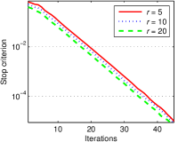
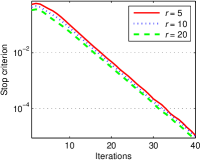
Refer to caption
Refer to caption
(a) Stop criterion: (S+L)1/2subscriptS+L12(\textup{S+L})_{1/2} (left) and (S+L)2/3subscriptS+L23(\textup{S+L})_{2/3} (right)
Refer to caption
Refer to caption
(b) RSE: (S+L)1/2subscriptS+L12(\textup{S+L})_{1/2} (left) and (S+L)2/3subscriptS+L23(\textup{S+L})_{2/3} (right)
Figure 14: Convergence behavior of our (S+L)1/2subscriptS+L12(\textup{S+L})_{1/2} and (S+L)2/3subscriptS+L23(\textup{S+L})_{2/3} methods for the cases of the matrix rank 5, 10 and 20.

Robustness

Like the other non-convex methods such as PSVT and Unifying, the most important parameter of our methods is the rank parameter d𝑑d. To verify the robustness of our methods with respect to d𝑑d, we report the RSE results of PSVT, Unifying and our methods on corrupted matrices with outlier ratio 10% in Fig. 15(a), in which we also present the results of the baseline method, LpSq [31]. It is clear that both our methods perform much more robust than PSVT and Unifying, and consistently yield much better solutions than the other methods in all settings.
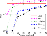
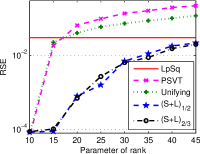
Refer to caption
Refer to caption
(a) RSE vs. d𝑑d: 200×200200200200\!\times\!200 (left) and 500×500500500500\!\times\!500 (right)
Refer to caption
Refer to caption
(b) RSE vs. λ𝜆\lambda: 200×200200200200\!\times\!200 (left) and 500×500500500500\!\times\!500 (right)
Figure 15: Comparison of RSE results on corrupted matrices with different rank parameters (a) and regularization parameters (b).

To verify the robustness of both our methods with respect to another important parameter (i.e. the regularization parameter λ𝜆\lambda), we also report the RSE results of our methods on corrupted matrices with outlier ratio 10% in Fig. 15(b). Note that the rank parameter of both our methods is computed by our rank estimation procedure. From the resutls, one can see that both our methods demonstrate very robust performance over a wide range of the regularization parameter, e.g. from 104superscript10410^{-4} to 100superscript10010^{0}.

TABLE IV: Information of the surveillance video sequences used in our experiments.
Datasets Bootstrap Hall Lobby Mall WaterSurface
Size×absent\times\sharpframes [120,160]×10001201601000[120,160]\times 1000 [144,176]×10001441761000[144,176]\times 1000 [128,160]×10001281601000[128,160]\times 1000 [256,320]×600256320600[256,320]\times 600 [128,160]×500128160500[128,160]\times 500
Description Crowded scene Crowded scene Dynamic foreground Crowded scene Dynamic background
Refer to caption
Refer to caption
Figure 16: The text removal results (including RSE (left) and F-measure (right)) of LpSq [31], Unifying [49] and our methods with different rank parameters.
Refer to caption
Refer to caption
Refer to caption
Refer to caption
Refer to caption
Refer to caption
Refer to caption
Refer to caption
Refer to caption
Refer to caption
Refer to caption
Refer to caption
Refer to caption
Refer to caption
Refer to caption
Refer to caption
Refer to caption
Refer to caption
Refer to caption
Refer to caption
Refer to caption
Refer to caption
Refer to caption
Refer to caption
Refer to caption
Refer to caption
Refer to caption
Refer to caption
Refer to caption
Refer to caption
Refer to caption
Refer to caption
Refer to caption
Refer to caption
Refer to caption
Refer to caption
Refer to caption
Refer to caption
Refer to caption
Refer to caption
Refer to caption
Refer to caption
Refer to caption
(a) ​Input, ​segmentation
Refer to caption
(b) RegL1 [16]
Refer to caption
(c) Unifying [49]
Refer to caption
(d) factEN [15]
Refer to caption
(e) (S+L)1/2subscriptS+L12(\textup{S+L})_{1/2}
Refer to caption
(f) (S+L)2/3subscriptS+L23(\textup{S+L})_{2/3}
Figure 17: Background and foreground separation results of different algorithms on the Hall, Mall, Lobby and WaterSurface data sets. The one frame with missing data of each sequence (top) and its manual segmentation (bottom) are shown in (a). The results by different algorithms are presented from (b) to (f), respectively. The top panel is the recovered background and the bottom panel is the segmentation.

Text Removal

We report the text removal results of our methods with varying rank parameters (from 10 to 40), as shown in Fig. 16, where the rank of the original image is 10. We also present the results of the baseline method, LpSq [31]. The results show that our methods significantly outperform the other methods in terms of RSE and F-measure, and they perform much more robust than Unifying with respect to the rank parameter.

Moving Object Detection

We present the detailed descriptions for five surveillance video sequences: Bootstrap, Hall, Lobby, Mall and WaterSurface data sets, as shown in Table IV. Moreover, Fig. 17 illustrates the foreground and background separation results on the Hall, Mall, Lobby and WaterSurface data sets.

Image Inpainting

In this part, we first reported the average PSNR results of two proposed methods (i.e., D-N and F-N) with different ratios of random missing pixels from 95% to 80%, as shown in Fig. 18. Since the methods in [19, 38] are very slow, we only present the average inpainting results of APGL242424http://www.math.nus.edu.sg/~mattohkc/NNLS.html [43] and WNNM252525http://www4.comp.polyu.edu.hk/~cslzhang/ [46], both of which use the fast SVD strategy and need to compute only partical SVD instead of the full one. Thus, APGL and WNNM are usually much faster than the methods [19, 38]. Considering that only a small fraction of pixels are randomly selected, thus we conducted 50 independent runs and report the average PSNR and standard deviation (std). The results show that both our methods consistently outperform APGL [43] and WNNM [46] in all the settings. This experiment actually shows that both our methods have even greater advantage over existing methods in the cases when the numer of observed pixels is very limited, e.g., 5% observed pixels.
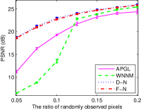
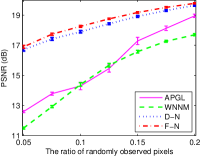
Refer to caption
(a) Image 1
Refer to caption
(b) Image 2
Refer to caption
(c) Image 3
Refer to caption
(d) Image 4
Refer to caption
(e) Image 5
Refer to caption
(f) Image 6
Refer to caption
(g) Image 7
Refer to caption
(h) Image 8
Figure 18: The average PSNR and standard deviation of APGL [43], WNNM [46] and both our methods for image inpainting vs. fraction of observed pixels (best viewed in colors).

As suggested in [38], we set d=9𝑑9d\!=\!9 for our two methods and TNNR262626https://sites.google.com/site/zjuyaohu/ [38]. To evaluate the robustness of our two methods with respect to their rank parameter, we report the average PSNR and standard deviation of two proposed methods with varying rank parameter d𝑑d from 7 to 15, as shown in Fig. 19. Moreover, we also present the average inpainting results of TNNR [38] over 50 independent runs. It is clear that two proposed methods perform much more robust than TNNR with repsect to the rank parameter.
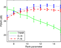
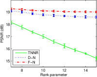
Refer to caption
(a) Image 1
Refer to caption
(b) Image 2
Refer to caption
(c) Image 3
Refer to caption
(d) Image 4
Refer to caption
(e) Image 5
Refer to caption
(f) Image 6
Refer to caption
(g) Image 7
Refer to caption
(h) Image 8
Figure 19: The average PSNR and standard deviation of TNNR [38] and both our methods for image inpainting vs. the rank parameter (best viewed in colors).