Multiple-shot and unambiguous discrimination of von Neumann measurements
Abstract
We present an in-depth study of the problem of multiple-shot discrimination of von Neumann measurements in finite-dimensional Hilbert spaces. Specifically, we consider two scenarios: minimum error and unambiguous discrimination. In the case of minimum error discrimination, we focus on discrimination of measurements with the assistance of entanglement. We provide an alternative proof of the fact that all pairs of distinct von Neumann measurements can be distinguished perfectly (i.e. with the unit success probability) using only a finite number of queries. Moreover, we analytically find the minimal number of queries needed for perfect discrimination. We also show that in this scenario querying the measurements in parallel gives the optimal strategy, and hence any possible adaptive methods do not offer any advantage over the parallel scheme. In the unambiguous discrimination scenario, we give the general expressions for the optimal discrimination probabilities with and without the assistance of entanglement. Finally, we show that typical pairs of Haar-random von Neumann measurements can be perfectly distinguished with only two queries.
1 Introduction
With the recent technological progress, quantum information science is not merely a collection of purely theoretical ideas anymore. Indeed, quantum protocols of increasing degree of complexity are currently being implemented on more and more complicated quantum devices [1, 2] and are expected to soon yield practical solutions to some real-world problems [3]. This situation motivates the need for certification and benchmarking of various building-blocks of quantum devices [4, 5, 6] (see [7] for a recent review). Discrimination or quantum hypothesis testing constitute one of the paradigms for assessing the quality of parts of quantum protocols [8, 9, 10, 11, 12]. In this work, we present a comprehensive study of various scenarios of discrimination of von Neumann measurements on a finite-dimensional Hilbert space. Here, by von Neumann measurements, we understand fine-grained projective measurements. Such measurements are vital for most of the protocols appearing in quantum information and quantum computing. In fact, even the most general quantum measurements are typically implemented using projective measurements performed on enlarged Hilbert space via the so-called Naimark construction [13]. Due to imperfections present in currently available quantum devices [3] and increased complexity associated with Naimark construction, standard projective measurements, such as the computational basis measurement, are the most common measurements implemented currently on quantum processors. It is important to point out that despite their relative simplicity, the actual implementation of projective measurements on quantum hardware is imperfect. For example, in a recent demonstration of quantum computational supremacy (advantage) by the collaboration of Google and UCBS [14] the researchers reported single-qubit measurement errors that are of order of a few percents. This motivates the interest in certification strategies tailored specifically to von-Neumann measurements.
The general problem of quantum channel discrimination has attracted a lot of attention in recent years. One of the first results was the study of discrimination of unitary operators [15, 16]. Later, this has been extended to various settings, such as multipartite unitary operations [17] and the case of discrimination among more than two unitary channels [18]. In the work [19] the authors formulated necessary and sufficient conditions under which quantum channels can be perfectly discriminated. Further works investigated the adaptive [20, 21, 22, 23] and parallel [24] schemes for discrimination of channels. Finally, some asymptotic results on discrimination of typical quantum channels in large dimensions were obtained in [25]. Discrimination of quantum measurements, being a subset of quantum channels, is thus of particular interest. Some of the earliest results on this topic involve condition on perfect discrimination of two measurements [26, 27, 28, 29, 30]
We are interested in the following problem. Imagine we have an unknown device hidden in a black box. We know it performs one of the two possible von Neumann measurements, either or . Generally, whenever a quantum state is sent through the box, the box produces, with probabilities predicted by quantum mechanics, classical labels corresponding to the measurement outcomes. Our goal is to find schemes that attain the optimal success probability for discrimination of measurements. The results contained in this work concern the following two scenarios:
Minimum error discrimination— In this setting, we are allowed to use the black box containing von Neumann measurement many times. Furthermore, we can prepare any input state with an arbitrarily large quantum memory (i.e., we can use ancillas of arbitrarily large dimension), and we can perform any channels between usages of the black box. This allows us to implement both parallel (see Fig. 1) as well as adaptive discrimination strategies (see Fig. 2). We focus on the case of entanglement-assisted discrimination. Our main finding is that in the multiple-shot scenario, adaptive strategies do not offer any advantage over parallel queries. Moreover, we derive an explicit dependence of the diamond norm distance in the multiple-shot scenario as a function of the diamond norm in the single-shot setting. As a consequence, we recover a known result [26] stating that given sufficiently many queries, every pair of different von Neumann measurements can be distinguished perfectly (i.e. with zero error probability).


Unambiguous discrimination— This scenario is an analogue to the well-known scheme of unambiguous state discrimination [31]. Namely, for every query to the black box, the decision procedure outputs , , or the inconclusive answer. The latter means that the user cannot decide which measurement was contained in the black box. Importantly, we require that the procedure cannot wrongly identify the measurement (see Fig. 3). Our main contribution to this problem is the derivation of the general schemes, which attain the optimal success probability both with and without the assistance of entanglement. Interestingly, we find that optimal success probability for unambiguous discrimination of projective measurements with the assistance of entanglement is functionally related to the diamond norm distance , which quantifies distinguishability of with the assistance of entanglement but without requiring unambiguous results. The specific formula is given by
| (1) |
and its geometric interpretation is presented in Fig. 4. Finally, we also present simple formulas for the optimal discrimination probability of von Neumann measurements for qubits.


Relation with classical channels— Let us contrast our results with transformations mapping probability distributions to probability distributions, that is classical channels. In this setting, we know that if such channels cannot be perfectly distinguished in one shot, they cannot be distinguished perfectly in any finite number of uses. What we can do is to study the asymptotic behavior of error probability when the number of applications of the channel tends to infinity. The error probability, formulated in the language of the hypothesis testing of two distributions, decays exponentially, and the optimal exponential error rate, depending on a formulation, is given by the Stein bound, the Chernoff bound, the Hoeffding bound, and the Han-Kobayashi bound, see [32] and references therein. In the case of distinct von Neumann measurements and entanglement-assisted discrimination, we show that one can perform perfect discrimination with the use of a finite number of queries. Therefore, in contrary to the classical channels, we do not have to consider the exponential error rate, as the error probability drops to zero in a finite number of tries.
This work is organized as follows. In Section 2, we give a survey of the main concepts and notation used throughout this work (including the basic background on discrimination of quantum channels and measurements). Then, in Section 3, we present our results for the scenario of multiple-shot minimum error measurement discrimination. Theorem 1 therein expresses the minimum error in the parallel discrimination scheme as a function of the minimum error in the single-shot discrimination scheme. Theorem 3 gives the upper bound on the probability of correct discrimination of a generic pair of von Neumann measurements coming from the Haar distribution. The following Section 4 contains the results concerning the unambiguous discrimination of quantum measurements. The main result of this section is formulated as Theorem 4, which states the optimal success probability of unambiguous discrimination with the assistance of entanglement. Lastly, in Section 5 we summarize our results and give some directions for future research.
2 Preliminaries and main concepts
By we will denote the set of quantum states on . Let denote the set of all linear operators acting from to . For brevity we will put . A quantum channel is a linear mapping which is completely positive and trace-preserving. The former means that for every we have , while the latter means for every . A set of generalized measurements (POVMs) will be denoted by . A general quantum measurement on is a tuple of positive semidefinite operators111In this paper we restrict our attention to measurements with a finite number of outcomes. on that add up to identity on i.e. with and . If a quantum state is measured by a measurement , then the outcome is obtained with the probability (Born rule). Therefore, a quantum measurement can be uniquely identified with a quantum channel
| (2) |
where states are perfectly distinguishable (orthogonal) pure states that can be regarded as states describing the state of a classical register. In what follows we will abuse the notation and simply treat quantum measurements (denoted by symbols , …) as quantum channels having the classical outputs. Using this interpretation one can readily use the results concerning the discrimination of quantum channels for generalized measurements. In particular, for entanglement-assisted discrimination of quantum channels we have a classic result due to Helstrom [33]. It states that the probability of correct discrimination between two quantum channels and is given by
| (3) |
where denotes the diamond norm of the linear map . Any optimal is called a discriminator. Thus, if the value of the diamond norm of the difference of two channels is strictly smaller than two, then the two channels cannot be distinguished perfectly in a single-shot scenario.
In this work we will be concerned with von Neumann measurements i.e. projective and fine-grained measurements on a Hilbert space of a given dimension . Von Neumann measurements in are tuples of orthogonal projectors on vectors forming an orthonormal basis in i.e.
| (4) |
In what follows we will use to denote the measurement in the standard computational basis. We will also use to denote the von Neumann measurement in the basis for a unitary matrix . In other words, vectors from Eq.(4) are columns of the matrix . We also specify the subset of diagonal, unitary matrices. Consider now a general task of discriminating between two projective measurements , , and let be the optimal probability for discriminating between these measurements (both for minimum error and for unambiguous discrimination). Then, due to the unitary invariance of the discrimination problem and identity we obtain that . Therefore, for any discrimination of projective measurements, without loss of generality, we can limit ourselves to considering the problem of distinguishing between the measurement in the standard basis and another projective measurement . It is important to note that definition of measurement distinguishes projective measurements differing only by ordering of elements of the basis. Moreover, a set of unitary matrices specifies the same projective measurement, ie. for all .
Distinguishability of quantum measurements is strictly related to the distinguishability of unitary channels. The prominent result [34, 35] gives an expression which makes calculating the diamond norm of the difference of unitary channels , substantially easier. It says that the for a unitary matrix we have
| (5) |
where and denotes the numerical range of the operator . Building on this result, in [29] the following characterization of the diamond norm of the distance between von Neumann measurements was obtained
| (6) |
Therefore the distance between two von Neumann measurements is the minimal value of the diamond norm of the difference between optimally coherified channels [36]. Moreover, there is a simple condition which lets us check whether two measurements are perfectly distinguishable [29, 24, 26]. It holds that if and only if there exists a state such that
| (7) |
Equation (6) will be of significant importance throughout this work. We will also make use of the dephasing channel denoted . Finally, when talking about the eigenvalues of a unitary matrix , we will follow convention that are ordered by their phases, if for . The angle of the shortest arc containing all eigenvalues will be denoted by .
3 Minimum error discrimination
Multiple-shot minimum error discrimination is a natural generalization of the single-shot scheme studied in [29]. In this scenario we have access to multiple queries to quantum measurements which is mathematically equivalent to the problem of single-shot discrimination of channels acting on states defined on multiple-component Hilbert space (see Fig. 5). In the following sections will write shortly instead of .

As we described in the preceding section, the problem of distinguishing quantum measurements is intimately related to distinguishing unitary channels [29]. In what follows we leverage this result to prove a number of results regarding multiple-shot discrimination of von Neumann measurements.
3.1 Optimality of the parallel scheme
The authors of [37] showed that parallel discrimination scheme is optimal among all possible architectures for the case of discrimination of unitary channels. In this subsection we will prove a theorem which thesis is rendered in the spirit of the results obtained in [37], nevertheless, our theorem concerns the discrimination of von Neumann measurements. It is worth mentioning here that the optimality of the parallel scheme is no longer true when studying the discrimination of general (non-projective) POVMs. In the case of discrimination of POVMs with rank-one effects one may need to use adaptive discrimination scheme to obtain perfect distinguishability [23]. While considering the discrimination of von Neumann measurements, one could expect that we can improve the discrimination by performing some processing based on the obtained measurement’s labels. It appears that such processing will not improve the discrimination.
We will focus on the minimum error discrimination in the parallel scenario and our goal will be to characterize the probability of correct discrimination after queries to the black box. The first step is to extend Eq. (6) to the parallel setting. We study the form of the optimal matrix in the parallel scheme. The following theorem, which proof is presented in Appendix A, states that it has a tensor product form.
Theorem 1.
Let , and let be the corresponding von Neumann measurement on . Then we have the following equality
| (8) |
Now we are interested in calculating the number of usages of the black box required for perfect discrimination. Let us recall here that in the case of distinguishing unitary operations this can always be achieved in a finite number of steps [15]. A similar result is achievable in the case of distinguishing von Neumann measurements. Let be an optimal unitary matrix, that is a matrix for which
| (9) |
Now we compute the number of queries needed for perfect discrimination. We have already proven in Theorem 1 that if is the optimal matrix, then the matrix will also be optimal. Therefore, the value of diamond norm can be expressed as a function of . As long as , it holds that . The first time zero enters the numerical range is therefore equal to , where is an optimized version of i.e.
| (10) |
We summarize the above discussion as the Corollary below providing the value of in terms of .
Corollary 1.
Let , . The following holds
-
(i)
if , then ;
-
(ii)
if , then .
Another interesting property resulting from Theorem 1 and its proof is the amount of the discriminator’s entanglement with environment. The minimal dimension of an auxiliary system needed for optimal discrimination is equal to the rank of the input state. We found out that for the majority of von Neumann measurements it is sufficient when the dimension of the auxiliary system is either two or three. A more detailed discussion is presented in Appendix A after the proof of Theorem 1.
Eventually, we are in the position to prove the optimality of parallel discrimination scheme, which we present as the following theorem.
Theorem 2.
Let . Consider the distinguishability of general quantum network with uses of the black box in which there is one of two measurements - either or . Then the probability of correct distinction cannot be better then in the parallel scenario.
Proof.
Without loss of generality we may assume that the processing is performed using only unitary operations. Indeed, using Stinespring dilation theorem, any channel might be represented via a unitary channel on a larger system followed by the partial trace operation. What is left to observe is that for arbitrary bipartite matrix .

The sequential scheme of discrimination of von Neumann measurements is shown in Fig. 6 and can be expressed as a channel
| (11) |
associated with a matrix . Here is the dephasing channel on subsystems . The channel is shown in Fig. 7 and the exact form of this transformation can be found in Appendix B.

Assuming that matrix is optimal, that is , we have . Hence, we may calculate the distance between and as
| (12) |
where we maximize over states of appropriate dimensions. The induced trace norm is monotonically decreasing under the action of channels and this gives us first inequality. The second one follows from the optimality of the parallel scheme of distinguishing unitary channels [37]. Therefore, the adaptive scenario does not give any advantage over the parallel scheme. ∎
3.2 Discrimination of random measurements
The structural characterization of multiple-shot discrimination of von Neumann measurements given above allows us to draw strong conclusions about distinguishability of generic pairs of von Neumann measurements. In this work we restrict our attention to pairs of measurements distributed independently according to the natural distribution coming from the Haar measure [38].
Theorem 3.
Consider two independently distributed Haar-random von Naumann measurements on , i.e. , where . Let be the optimal probability of discrimination measurements and using two queries and assistance of entanglement. Then, we have the following bound
| (13) |
In other words, in the limit of large dimensions , typical Haar-random von Neumann measurements are perfectly distinguishable with the usage of two queries and assistance of entanglement (the probability that they cannot be perfectly distinguished is exponentially suppressed as a function of ).
Proof.
From the unitary invariance of the Haar measure and the symmetry of the problem of measurement discrimination it follows that the distribution of the random variable is identical to that of . Consequently, we have
| (14) |
From Corollary 1 it follows that the condition implies and consequently we have also perfect discrimination of two copies of measurements: . Therefore we have
| (15) |
Using now the characterization given in Eq.(6) in conjunction with the formula in Eq.(5) we obtain (note that ). Using this and simple algebra we get
| (16) |
The right-hand side of the above inequality can be computed exactly using the property that for Haar-distributed the random variable is distributed according to the beta distribution (see for instance Eq. (9) in [39]). The simple integration gives , which together with Eq.(14) gives the claimed result. ∎
4 Unambiguous discrimination
The unambiguous discrimination of measurements and can be understood as unambiguous discrimination [31] of states generated by the corresponding channels. Specifically, for a fixed input state , the output states can be unambiguously discriminated using the measurement strategy , where the first two effects represent conclusive answers and the last one corresponds to the inconclusive output of the procedure. For equal a priori probabilities of occurrence of and , as well as fixed (possibly entangled) and , the success probability is given by
| (17) |
where additionally the unambiguity condition has to be satisfied:
| (18) |
The optimal success probability of unambiguous discrimination of measurements can be now defined as the maximum of (17) over all strategies. Formally, we have
| (19) |
where is a three-outcome measurement on that satisfies constrains (18) end is a state on the extended Hilbert space .
4.1 Unambiguous discrimination with assistance of entanglement
In this subsection we present our main result which gives the probability of unambiguous discrimination with the use of entanglement This is presented as Theorem 4 while its proof is postponed to Appendix C. Aside from giving a simple expression for this probability, this result reduces the problem of unambiguous measurement discrimination to a convex optimization task and gives a simple relationship between the diamond norm and the probability of unambiguous discrimination.
Theorem 4.
The optimal success probability of unambiguous discrimination between von Neumann measurements and is given by
| (20) |
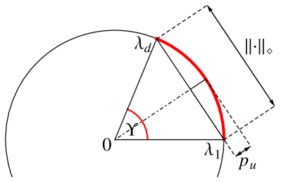
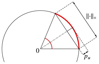
The results coming from Theorem 1 and Theorem 4 give a nice geometric interpretation for the relationship between the diamond norm and the probability of unambiguous discrimination. This is depicted in Fig. 8. We start with a von Neumann measurement in a basis given by some unitary matrix and try to distinguish it from the measurement in the computational basis. We assume that is optimal and denote ’s eigenvalues as ordered according to their phases and use the symbol to denote the angle between two most distant eigenvalues and . The dependence of the diamond norm and probability of unambiguous discrimination is clearly shown.
Remark 1.
The above calculations can be easily extended to the case of parallel discrimination scheme. It suffices to substitute with and then we obtain that
| (21) |
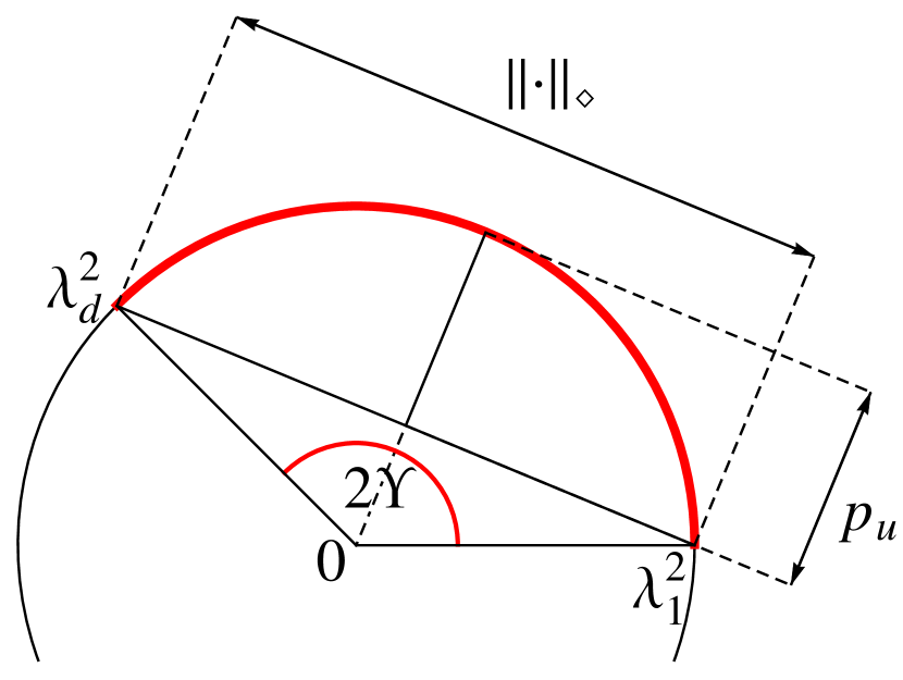
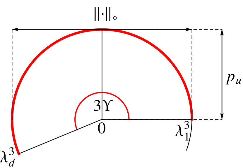
Basing on Remark 1, we note that the angle increases in the multiple-shot case with the number of queries. This is depicted in Fig. 9 for two- and three-shots scenarios.
In the general scheme we are allowed to use conditional unitary transformations after each measurement, thus our setting for discrimination is the same as presented in Fig. 6 and Fig. 7. Similarly to the multiple-shot minimum error discrimination, we will show that adaptive discrimination scheme does not give any advantage over the parallel one for unambiguous discrimination. We state this formally in the following theorem, which proof is moved to Appendix D.
Theorem 5.
Let . Consider the unambiguous discrimination of general quantum network with uses of the black box in which there is one of two measurements - either or . Then the probability of correct distinction cannot be better then in the parallel scenario.
4.2 Unambiguous discrimination without assistance of entanglement
In this subsection we provide a brief discussion on a special case of unambiguous discrimination without the utilization of entangled states. We will use the following notation. Let . For given unitary matrix , we define and . We set to be the orthogonal projector onto , where denote the complements of and respectively. The following theorem states the optimal success probability of unambiguous discrimination without the use of entanglement.
Theorem 6.
The optimal success probability of unambiguous discrimination, without the use of entanglement, between von Neumann measurements and is given by
| (22) |
with defined as above.
The proof of this theorem is presented in Appendix E.
Remark.
Corollary 2.
In the case of qubit measurements, the optimal probability of unambiguous discrimination of and is given by the following (discontinuous) function
| (24) |
In both cases the optimal input state can be chosen to be .
The following corollary states that in the qubit case the unambiguous discrimination with the assistance of entanglement always outperforms the unambiguous discrimination without the use of entanglement. On top of that, the special cases for which the use of entanglement does not give any advantage are described.
Corollary 3.
Let and be two von Neumann measurements on a qubit. If , then the probability of entanglement-assisted unambiguous discrimination is given by
| (25) |
and it is always greater then the probability without assistance of entanglement
| (26) |
Moreover, if , then .
Remark.
The above considerations can be extended to unambiguous discrimination of multiple copies of von Neumann measurements applied in parallel. To this end, if we have access to parallel queries to a black box measurement, it suffices to replace unitaries by and by in the above computations. Interestingly, in the contrast to unambiguous discrimination of quantum states [31], having access to two copies of black box measurement, sometimes allows attaining perfect discrimination. Specifically, consider the problem of discriminating between and , where . Explicit computation shows that by taking the input state as allows us to perfectly distinguish between and .
5 Conclusions
We have presented a comprehensive treatment of the problem of discrimination of von Neumann measurements. First of all, we showed an alternative proof of the fact that for any pair of measurements and , , there exists a finite number of uses of the black box which allows us to achieve perfect discrimination. Moreover, we calculated the exact value of the diamond norm for given . This is formally stated in Corollary 1. We also proved that the parallel discrimination scheme is optimal in the scenario of multiple-shot minimum error discrimination of von Neumann measurements (see Theorem 2).
Moreover, we studied unambiguous discrimination of von Neumann measurements. Our main contribution to this problem was the derivation of the general schemes that attain the optimal success probability both with (see Theorem 4) and without (see Theorem 6) the assistance of entanglement. Interestingly, for entanglement-assisted unambiguous discrimination the optimal success probability is functionally related to the corresponding success probability for minimum error discrimination. Finally, we show that the parallel scheme is also optimal for unambiguous discrimination.
There are many interesting directions for further study that still remain to be explored. Below we list the most important (in our opinion) open research problems:
- •
-
•
Systematical study of the problem of unambiguous discrimination of projective measurements in the multiple-shot regime.
-
•
Can typical pairs of Haar-random projective measurements on be discriminated perfectly using only one query and the assistance of entanglement as ?
-
•
How much entanglement is needed to attain the optimal success probability of multiple-shot discrimination of generic projective measurements on ? In the same scenario, is it necessary to adopt the final measurement to the pair of measurements to be discriminated?
Acknowledgements
We would like to thank Alessandro Bisio and Giulio Chiribella for fruitful discussions.
This work was supported by the Polish National Science Centre under project numbers 2016/22/E/ST6/00062 (ZP, AK, RK) and 2015/18/E/ST2/ 00327 (ŁP). MO acknowledges the support of Homing programme of the Foundation for Polish Science co-financed by the European Union under the European Regional Development Fund.
References
- [1] J. Carolan, C. Harrold, C. Sparrow, E. Martín-López, N. J. Russell, J. W. Silverstone, P. J. Shadbolt, N. Matsuda, M. Oguma, M. Itoh, G. D. Marshall, M. G. Thompson, J. C. F. Matthews, T. Hashimoto, J. L. O’Brien, and A. Laing, “Universal linear optics,” Science, vol. 349, no. 6249, pp. 711–716, 2015.
- [2] S. Boixo, S. V. Isakov, V. N. Smelyanskiy, R. Babbush, N. Ding, Z. Jiang, M. J. Bremner, J. M. Martinis, and H. Neven, “Characterizing quantum supremacy in near-term devices,” Nature Physics, vol. 14, no. 6, pp. 595–600, 2018.
- [3] J. Preskill, “Quantum Computing in the NISQ era and beyond,” Quantum, vol. 2, p. 79, 2018.
- [4] E. Magesan, J. M. Gambetta, and J. Emerson, “Scalable and Robust Randomized Benchmarking of Quantum Processes,” Phyical Review Letters, vol. 106, p. 180504, 2011.
- [5] L. Aolita, C. Gogolin, M. Kliesch, and J. Eisert, “Reliable quantum certification of photonic state preparations,” Nature Communications, vol. 6, p. 8498, 2015.
- [6] J. R. Wootton, “Benchmarking of quantum processors with random circuits,” arxiv:1806.02736, 2018.
- [7] J. Eisert, D. Hangleiter, N. Walk, I. Roth, D. Markham, R. Parekh, U. Chabaud, and E. Kashefi, “Quantum certification and benchmarking,” Nature Reviews Physics, pp. 1–9, 2020.
- [8] A. Chefles, “Quantum state discrimination,” Contemporary Physics, vol. 41, no. 6, pp. 401–424, 2000.
- [9] S. M. Barnett and S. Croke, “Quantum state discrimination,” Advances in Optics and Photonics, vol. 1, no. 2, pp. 238–278, 2009.
- [10] J. A. Bergou, “Discrimination of quantum states,” Journal of Modern Optics, vol. 57, no. 3, pp. 160–180, 2010.
- [11] J. Bae and L.-C. Kwek, “Quantum state discrimination and its applications,” Journal of Physics A: Mathematical and General, vol. 48, no. 8, p. 083001, 2015.
- [12] S. Pirandola, R. Laurenza, C. Lupo, and J. L. Pereira, “Fundamental limits to quantum channel discrimination,” npj Quantum Information, vol. 5, no. 1, pp. 1–8, 2019.
- [13] J. Watrous, The Theory of Quantum Information. Cambridge University Press, 2018.
- [14] F. Arute, K. Arya, R. Babbush, D. Bacon, J. C. Bardin, R. Barends, R. Biswas, S. Boixo, F. G. Brandao, D. A. Buell, et al., “Quantum supremacy using a programmable superconducting processor,” Nature, vol. 574, no. 7779, pp. 505–510, 2019.
- [15] A. Acín, “Statistical distinguishability between unitary operations,” Physical Review Letters, vol. 87, no. 17, p. 177901, 2001.
- [16] R. Duan, Y. Feng, and M. Ying, “Entanglement is not necessary for perfect discrimination between unitary operations,” Physical Review Letters, vol. 98, no. 10, p. 100503, 2007.
- [17] R. Duan, Y. Feng, and M. Ying, “Local distinguishability of multipartite unitary operations,” Physical Review Letters, vol. 100, no. 2, p. 020503, 2008.
- [18] G. Chiribella, G. M. D’Ariano, and M. Roetteler, “Identification of a reversible quantum gate: assessing the resources,” New Journal of Physics, vol. 15, no. 10, p. 103019, 2013.
- [19] R. Duan, Y. Feng, and M. Ying, “Perfect distinguishability of quantum operations,” Physical Review Letters, vol. 103, no. 21, p. 210501, 2009.
- [20] A. W. Harrow, A. Hassidim, D. W. Leung, and J. Watrous, “Adaptive versus nonadaptive strategies for quantum channel discrimination,” Physical Review A, vol. 81, no. 3, p. 032339, 2010.
- [21] T. P. Cope and S. Pirandola, “Adaptive estimation and discrimination of Holevo-Werner channels,” Quantum Measurements and Quantum Metrology, vol. 4, no. 1, pp. 44–52, 2017.
- [22] S. Pirandola and C. Lupo, “Ultimate precision of adaptive noise estimation,” Physical Review Letters, vol. 118, no. 10, p. 100502, 2017.
- [23] A. Krawiec, Ł. Pawela, and Z. Puchała, “Discrimination of POVMs with rank-one effects,” Quantum Information Processing, vol. 19, no. 12, pp. 1–12, 2020.
- [24] R. Duan, C. Guo, C.-K. Li, and Y. Li, “Parallel distinguishability of quantum operations,” in 2016 IEEE International Symposium on Information Theory (ISIT), pp. 2259–2263, IEEE, 2016.
- [25] I. Nechita, Z. Puchała, Ł. Pawela, and K. Życzkowski, “Almost all quantum channels are equidistant,” Journal of Mathematical Physics, vol. 59, no. 5, p. 052201, 2018.
- [26] Z. Ji, Y. Feng, R. Duan, and M. Ying, “Identification and distance measures of measurement apparatus,” Physical Review Letters, vol. 96, no. 20, p. 200401, 2006.
- [27] G. M. D’Ariano, P. L. Presti, and M. G. Paris, “Using entanglement improves the precision of quantum measurements,” Physical Review Letters, vol. 87, no. 27, p. 270404, 2001.
- [28] G. Chiribella, G. M. D’Ariano, and P. Perinotti, “Memory Effects in Quantum Channel Discrimination,” Physical Review Letters, vol. 101, p. 180501, oct 2008.
- [29] Z. Puchała, Ł. Pawela, A. Krawiec, and R. Kukulski, “Strategies for optimal single-shot discrimination of quantum measurements,” Physical Review A, vol. 98, p. 042103, 2018.
- [30] M. Sedlák and M. Ziman, “Optimal single-shot strategies for discrimination of quantum measurements,” Physical Review A, vol. 90, no. 5, p. 052312, 2014.
- [31] D. Dieks, “Overlap and distinguishability of quantum states,” Physics Letters A, vol. 126, no. 5, pp. 303 – 306, 1988.
- [32] M. Hayashi, “Discrimination of two channels by adaptive methods and its application to quantum system,” IEEE Transactions on Information Theory, vol. 55, no. 8, pp. 3807–3820, 2009.
- [33] C. W. Helstrom, Quantum Detection and Estimation Theory. Elsevier, 1976.
- [34] G. Chiribella, G. M. D’Ariano, and P. Perinotti, “Theoretical framework for quantum networks,” Physical Review A, vol. 80, no. 2, p. 022339, 2009.
- [35] A. Bisio, G. Chiribella, G. D’Ariano, and P. Perinotti, “Quantum networks: general theory and applications,” Acta Physica Slovaca. Reviews and Tutorials, vol. 61, no. 3, pp. 273–390, 2011.
- [36] K. Korzekwa, S. Czachórski, Z. Puchała, and K. Życzkowski, “Coherifying quantum channels,” New Journal of Physics, vol. 20, no. 4, p. 043028, 2018.
- [37] G. Chiribella, G. M. D’Ariano, and P. Perinotti, “Memory effects in quantum channel discrimination,” Physical Review Letters, vol. 101, no. 18, p. 180501, 2008.
- [38] I. Bengtsson and K. Życzkowski, Geometry of quantum states: an introduction to quantum entanglement. Cambridge University Press, 2017.
- [39] K. Życzkowski and H.-J. Sommers, “Truncations of random unitary matrices,” Journal of Physics A: Mathematical and General, vol. 33, no. 10, p. 2045, 2000.
- [40] R. Piziak, P. Odell, and R. Hahn, “Constructing projections on sums and intersections,” Computers Mathematics with Applications, vol. 37, no. 1, pp. 67–74, 1999.
- [41] M. Oszmaniec, L. Guerini, P. Wittek, and A. Acín, “Simulating Positive-Operator-Valued Measures with Projective Measurements,” Physical Review Letters, vol. 119, p. 190501, Nov 2017.
- [42] L. Guerini, J. Bavaresco, M. Terra Cunha, and A. Acín, “Operational framework for quantum measurement simulability,” Journal of Mathematical Physics, vol. 58, no. 9, p. 092102, 2017.
- [43] F. Hausdorff, “Der Wertvorrat einer Bilinearform,” Mathematische Zeitschrift, vol. 3, no. 1, pp. 314–316, 1919.
- [44] O. Toeplitz, “Das algebraische Analogon zu einem Satze von Fejér,” Mathematische Zeitschrift, vol. 2, no. 1-2, pp. 187–197, 1918.
- [45] G. Jaeger and A. Shimony, “Optimal distinction between two non-orthogonal quantum states,” Physics Letters A, vol. 197, no. 2, pp. 83–87, 1995.
Appendix A Proof of Theorem 1
In this appendix we will begin with quoting two lemmas from [29] which contribute the main part of the proof of Theorem 1. The first lemma states that a function has a saddle point. The second lemma gives an equivalent condition to the existence of the saddle point and presents the form of the optimal state. Then, we present the proof of Theorem 1 and a short discussion about the amount of entanglement needed for the discrimination.
Lemma 1 (Lemma 4 from [29]).
Let us fix a unitary matrix . Then,
| (27) |
Lemma 2 (Lemma 5 from [29]).
Let us fix a unitary matrix and
-
•
and ,
-
•
,
-
•
denote the most distant pair of eigenvalues of
-
•
, denote the projectors on the subspaces spanned by the eigenvectors corresponding to , .
Then, the function has a saddle point in i.e.
| (28) |
if and only if there exist states such that
-
•
,
-
•
,
-
•
.
Moreover, if the above holds, then the state satisfying Eq. (28) can be chosen as .
Proof of Theorem 1.
In the first step of the proof assume that and are perfectly distinguishable in a single-shot scenario i.e.
| (29) |
This trivially implies that for each the measurements and are perfectly distinguishable and it holds that
| (30) |
which proves the thesis of the theorem in this case.
Now, consider the second case when and are not perfectly distinguishable using a single query. Then, according to equality
| (31) |
there exists an optimal matrix such that and .
The general proof strategy is to utilize the Lemma 2 in order to construct optimal discriminator for measurements and . Hence we start by establishing that the assumptions of this lemma are fulfilled. This will follow from Lemma 1. According to it the function has a saddle point. Let us remind that , where . Due to equality we have
| (32) |
Hence using the property that the numerical range is a convex set [43, 44] we obtain
| (33) |
Therefore the former assumptions of Lemma 2 are satisfied for the matrix and hence it is possible to take states , which fulfill the latter conditions of this Lemma.
To complete the proof we will separately study two cases. In the first one, we assume that POVMs and are not perfectly distinguishable using queries i.e. . Hence, as , then
| (34) |
and lie on the subspaces spanned by the eigenvectors of the matrix eigenvalues and , respectively. Consequently, we fulfilled the latter assumptions of Lemma 2 and the reverse implication of this Lemma states that the unitary matrix is optimal and for it holds that
| (35) |
Hence
| (36) |
and eventually
| (37) |
In the second case, let . Let us consider the situation when is the first index for which this happens, which means that .
If the measurements in question can be perfectly distinguished with queries, then we have and there exists a probability vector such that
| (38) |
Define a state
| (39) |
We will show that . Indeed
| (40) |
Thus from Proposition 3 form [29] the condition implies that , and hence
| (41) |
For , the equality implies that . Therefore
| (42) |
which completes the proof. ∎
Let us discuss the amount of the discriminator’s entanglement with environment. Note that the minimal dimension of an auxiliary system needed for optimal discrimination is equal to the rank of the state . One special case involves the situation , where . In the best case, when eigenvalues and are not degenerated, the states are pure, hence . On the other hand, when the spectrum of contains only and , then the rank of can be roughly upper-bounded by .
The situation is more complicated to analyze, due to lack of an analytic form of the discriminator in a general case. However, finding a pair of not degenerated eigenvalues saturating the latter assumptions of Lemma 2 will lead to , where is defined as in Eq. (39) and we check its optimality in the same manner as in Eq. (40).
Appendix B Explicit form of the matrix
The matrix is a general operation which allows for adaptive information processing in the sequential discrimination scenario of von Neumann measurements. It consists of a sequence of unitary matrices acting successively on given registers interlacing with classically controlled unitary operations . The explicit form of the matrix is given by
| (43) |
Appendix C Proof of Theorem 4
Proof of Theorem 4.
Assume that a black-box measurement ( or ) acts on a system extended by the ancilla space (of some dimension ). Without loss of generality we take the pure input state i.e. . Let be a matrix such that . The action of the channels and on can be expressed as
| (44) |
where we treat measurements and as a measure and prepare channels of the form .
As for any Hermitian operator and any measurement we have
| (45) |
where is a dephasing channel. Hence we can restrict our attention to considering measurements which effects have block-diagonal structure, that is
| (46) |
where is a POVM on associated with a measure and prepare channel. From Eq.(44) we see that upon obtaining the label , the state of the auxiliary subsystem is either
| (47) |
when measurement was performed, or it is given by
| (48) |
if was implemented. In the above formulas are responsible for normalization. We assume that and (otherwise the specific outcome does not occur). We see that states , are pure and therefore the optimal measurements will be simply given by
| (49) |
for some choice of which guarantees the non-negativity of .
The probability of success in unambiguous discrimination of pure states with unequal a priori probabilities is given by [45]
| (50) |
where .
We will use the following upper bound
| (51) |
which can be verified directly by elementary calculations.
Let . The overlap between states of the auxiliary subsystem is given by
| (52) |
while a priori probabilities of upon obtaining label are . Taking the above into account, we get that probability of success in unambiguous measurement on auxiliary subsystem, given that label was observed, can be bounded from above by
| (53) |
Therefore, the overall probability of success is bounded by
| (54) |
What is more, the above bound is tight. The situation when and are perfectly distinguishable is trivial to check. In the case when and are not perfectly distinguishable, then there exists a state which will give equal probabilities and for each label . This statement follows from Lemma 2, from which we take . ∎
Appendix D Proof of Theorem 5
Proof of Theorem 5.
We will assume that the unitary matrix is optimal, i.e. . Take an arbitrary input state . Let us denote
| (55) |
where and are defined as in Appendix B and are responsible for normalization. Repeating the calculation from the single-shot scenario from the proof in Appendix C we can upper-bound the probability of successful discrimination as follows
| (56) |
From the work [37] we know that there exists a state such that for all it holds that
| (57) |
Moreover, using optimality of and Lemma 1, the state can be chosen to satisfy . This leads to the desired inequality
| (58) |
∎
Appendix E Proof of Theorem 6
Proof of Theorem 6.
Let us fix the input state . Without loss of generality we can restrict our attention to measurements with diagonal effects (see Eq. (45) in Appendix C).
From the unambiguity condition we obtain that and . Therefore, the optimal measurements can be always chosen as projectors onto disjoint subsets of . The formula for the success probability reads
| (59) |
Importantly, the input state satisfies and . For fixed subsets , due to linearity, the maximum over equals , where denotes the operator norm and is the orthogonal projector onto . By optimizing over disjoint subsets we obtain the result.
∎
