Unbiased deep solvers for linear parametric PDEs

Abstract.

We develop several deep learning algorithms for approximating families of parametric PDE solutions. The proposed algorithms approximate solutions together with their gradients, which in the context of mathematical finance means that the derivative prices and hedging strategies are computed simulatenously. Having approximated the gradient of the solution one can combine it with a Monte-Carlo simulation to remove the bias in the deep network approximation of the PDE solution (derivative price). This is achieved by leveraging the Martingale Representation Theorem and combining the Monte Carlo simulation with the neural network. The resulting algorithm is robust with respect to quality of the neural network approximation and consequently can be used as a black-box in case only limited a priori information about the underlying problem is available. We believe this is important as neural network based algorithms often require fair amount of tuning to produce satisfactory results. The methods are empirically shown to work for high-dimensional problems (e.g. 100 dimensions). We provide diagnostics that shed light on appropriate network architectures.

Key words and phrases:
Monte Carlo method, Deep neural network, Control variates, Partial differential equations
2010 Mathematics Subject Classification:
65M75, 60H30, 91G60

1. Introduction

Numerical algorithms that solve PDEs suffer from the so-called “curse of dimensionality”, making it impractical to apply known discretisation algorithms such as finite differences schemes to solve high-dimensional PDEs. However, it has been recently shown that deep neural networks trained with stochastic gradient descent can overcome the curse of dimensionality [3, 6], making them a popular choice to solve this computational challenge in the last few years.

In this work, we focus on the problem of numerically solving parametric linear PDEs arising from European option pricing in high-dimensions. Let Bp,p1formulae-sequence𝐵superscript𝑝𝑝1B\subseteq\mathbb{R}^{p},p\geq 1 be a parameter space (for instance, in the Black–Scholes equation with fixed rate, B𝐵B is the domain of the volatility parameter). Consider v=v(t,x;β)𝑣𝑣𝑡𝑥𝛽v=v(t,x;\beta) satisfying

[tv+bxv+12tr[x2vσσ]cv](t,x;β)=0,v(T,x;β)=g(x;β),t[0,T],xd,βB.formulae-sequencedelimited-[]subscript𝑡𝑣𝑏subscript𝑥𝑣12trdelimited-[]superscriptsubscript𝑥2𝑣superscript𝜎𝜎𝑐𝑣𝑡𝑥𝛽0formulae-sequence𝑣𝑇𝑥𝛽𝑔𝑥𝛽formulae-sequence𝑡0𝑇formulae-sequence𝑥superscript𝑑𝛽𝐵\begin{split}&\bigg{[}\partial_{t}v+b\nabla_{x}v+\frac{1}{2}\text{tr}\left[\nabla_{x}^{2}v\sigma^{*}\sigma\right]-cv\bigg{]}(t,x;\beta)=0\,,\\ &v(T,x;\beta)=g(x;\beta)\,,\,\,\,t\in[0,T]\,,\,\,x\in\mathbb{R}^{d}\,,\,\,\beta\in B\,.\end{split} (1)

Here t[0,T]𝑡0𝑇t\in[0,T], xd𝑥superscript𝑑x\in\mathbb{R}^{d} and βB𝛽𝐵\beta\in B and b,σ,c𝑏𝜎𝑐b,\sigma,c and g𝑔g are functions of (t,x;β)𝑡𝑥𝛽(t,x;\beta) which specify the problem. The Feynman–Kac theorem provides a probabilistic representation for v𝑣v so that Monte Carlo methods can be used for its unbiased approximation in one single point (t,x;β)𝑡𝑥𝛽(t,x;\beta). What we propose in this work is a method for harnessing the power of deep learning algorithms to numerically solve (1) in a way that is robust even in edge cases when the output of the neural network is not of the expected quality, by combining them with Monte Carlo algorithms.

From the results in this article we observe that neural networks provide an efficient computational device for high dimensional problems. However, we observed that these algorithms are sensitive to the network architecture, parameters and distribution of training data. A fair amount of tuning is required to obtain good results. Based on this we believe that there is great potential in combining artificial neural networks with already developed and well understood probabilistic computational methods, in particular the control variate method for using potentially imperfect neural network approximations for finding unbiased solutions to a given problem, see Algorithm 1.

1.1. Main contributions

We propose three classes of learning algorithms for simultaneously finding solutions and gradients to parametric families of PDEs.

  1. i)

    Projection solver: See Algorithm 2. We leverage Feynman–Kac representation together with with the fact that conditional expectation can be viewed as an L2superscript𝐿2L^{2}-projection operator. The gradient can be obtained by automatic differentiation of already obtained approximation of the PDE solution.

  2. ii)

    Martingale representation solver: See Algorithm 3. This algorithm was inspired by Cvitanic et. al. [13] and Weinan et. al, Han et. al. [51, 22] and is referred to as deep BSDE solver. Our algorithm differs from [51] in that we approximate solution and its gradient at all the time-steps and across the entire space and parameter domains rather than only one space-time point. Furthermore we propose to approximate the solution-map and its gradient by separate networks.

  3. iii)

    Martingale control variates solver: Algorithms 4 and 5. Here we exploit the fact that martingale representation induces control variate that can produce zero variance estimator. Obviously, such control variate is not implementable but provides a basis for a novel learning algorithm for the PDE solution.

For each of these classes of algorithms we develop and test different implementation strategies. Indeed, one can either take one (large) network to approximate the entire family of solutions of (1) or take a number of (smaller) networks, where each of them approximates the solution at a time point in a grid. The former has the advantage that one can take arbitrarily fine time discretisation without increasing the overall network size. The advantage of the latter is that each learning task is simpler due to each network being smaller. One can further leverage the smoothness of the solution in time and learn the weights iteratively by initialising the network parameters to be those of the previous time step. We test both approaches numerically. At a high level all the algorithms work in path-dependent (non-Markovian) setting but there the challenge is an efficient method for encoding information in each path. This problem is solved in companion paper [45].

To summarise the key contribution of this work are:

  1. i)

    We derive and implement three classes of learning algorithms for approximation of parametric PDE solution map and its gradient.

  2. ii)

    We propose a novel iterative training algorithm that exploits regularity of the function we seek to approximate and allows using neural networks with smaller number of parameters.

  3. iii)

    The proposed algorithms are truly black-box in that quality of the network approximation only impacts the computation benefit of the approach and does not introduce approximation bias. This is achieved by combining the network approximation with Monte Carlo as stated in Algorithm 1.

  4. iv)

    Code for the numerical experiments presented in this paper is being made available on GitHub: https://github.com/msabvid/Deep-PDE-Solvers.

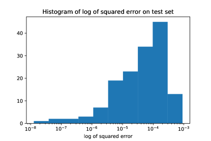
We stress the importance of point iii) above by directing reader’s attention to Figure 1, where we test generalisation error of trained neural network for the 5 dimensional family of PDEs corresponding to pricing a basket option under the Black–Scholes model. We refer reader to Example D.2 for details. We see that while the average error over test set is of order 105absentsuperscript105\approx 10^{-5}, the errors for a given input varies significantly. Indeed, it has been observed in deep learning community that for high dimensional problems one can find input data such that trained neural network that appears to generalise well (i.e achieves small errors on the out of training data) produces poor results [19].
Refer to caption
Figure 1. Histogram of mean-square-error of solution to the PDE on the test data set.

1.2. Literature review

Deep neural networks trained with stochastic gradient descent proved to be extremely successful in number of applications such as computer vision, natural language processing, generative models or reinforcement learning [36]. The application to PDE solvers is relatively new and has been pioneered by Weinan et. al, Han et. al. [51, 22, 47]. See also Cvitanic et. al. [13] for the ideas of solving PDEs with gradient methods and for direct PDE approximation algorithm. PDEs provide an excellent test bed for neural networks approximation because a) there exists alternative solvers e.g Monte Carlo b) we have well developed theory for PDEs, and that knowledge can be used to tune algorithms. This is contrast to mainstream neural networks approximations in text or images classification.

Apart from growing body of empirical results in literature on “Deep PDEs solvers”, [9, 28, 2, 31, 24] there has been also some important theoretical contributions. It has been proved that deep artificial neural networks approximate solutions to parabolic PDEs to an arbitrary accuracy without suffering from the curse of dimensionality. The first mathematically rigorous proofs are given in [20] and [32]. The high level idea is to show that neural network approximation to the PDE can be established by building on Feynman-Kac approximation and Monte-Carlo approximation. By checking that Monte-Carlo simulations do not suffer from the curse of dimensionality one can imply that the same is true for neural network approximation. Furthermore, it has been recently demonstrated in [27, 39] that noisy gradient descent algorithm used for training of neural networks of the form considered in [20, 32] induces unique probability distribution function over the parameter space which minimises learning. See [15, 10, 44, 48, 50, 23] for related ideas on convergence of gradient algorithms for overparametrised neural networks. This means that there are theoretical guarantees for the approximation of (parabolic) PDEs with neural networks trained by noisy gradient methods alleviating the curse of dimensionality.

An important application of deep PDE solvers is that one can in fact approximate a parametric family of solutions of a PDE. To be more precise let Bp𝐵superscript𝑝B\subseteq\mathbb{R}^{p}, p1𝑝1p\geq 1, be a parameter space. In the context of finance these, for example, might be initial volatility, volatility of volatility, interest rate and mean reversion parameters. One can approximate the parametric family of functions F(;β)βB𝐹subscript𝛽𝛽𝐵F(\cdot;\beta)_{\beta\in B} for an arbitrary range of parameters. This then allows for swift calibration of models to data (e.g options prices). This is particularly appealing for high dimensional problems when calibrating directly using noisy Monte-Carlo samples might be inefficient. This line of research gained some popularity recently and the idea has been tested numerically on various models and data sets [26, 37, 1, 49, 25, 30, 38]. There are some remarks that are in order. In the context of models calibration, while the training might be expensive one can do it offline, once and for good. One can also notice that training data could be used to produce a “look-up table” taking model parameters to prices. From this perspective the neural network, essentially, becomes an interpolator and a compression tool. Indeed the number of parameters of the network is much smaller than number of training data and therefore it is more efficient to store those. The final remark is that while there are other methods out there, such as Chebyshev functions, neural networks seem robust in high dimensions which make them our method of choice.

1.3. Notation

We denote by 𝒟𝒩𝒟𝒩\mathcal{DN} the set of all fully connected feedforward neural networks (see Appendix C). We also use [f]θ𝒟𝒩subscriptdelimited-[]𝑓𝜃𝒟𝒩\mathcal{R}[f]_{\theta}\in\mathcal{DN} with θκ𝜃superscript𝜅\theta\in\mathbb{R}^{\kappa} to denote a neural network with weights θ𝜃\theta approximating the function f:d0d1:𝑓superscriptsubscript𝑑0superscriptsubscript𝑑1f:\mathbb{R}^{d_{0}}\rightarrow\mathbb{R}^{d_{1}} for some d0,d1subscript𝑑0subscript𝑑1d_{0},d_{1}\in\mathbb{N}.

1.4. Outline

This paper is organised as follows. Section 2 provides theoretical underpinning for the derivation of all the algorithms we propose to solve (1). More specifically in Section 2.2 we combine the approximation of the gradient of the solution of the PDE resulting from the Deep Learning algorithms with Monte Carlo to obtain an unbiased approximation of the solution of the PDE. In Section 3, we describe the algorithms in detail.

Finally in Section 4 we provide numerical tests of the proposed algorithms. We empirically test these methods on relevant examples including a 100 dimensional option pricing problems, see Examples 4.4 and D.3. We carefully measure the training cost and report the variance reduction achieved.

Since we work in situation where the function approximated by neural network can be obtained via other methods (Monte-Carlo, PDE solution) we are able to test the how the expressiveness of fully connected artificial neural networks depends on the number of layers and neurons per layer. See Section D.1 for details.

2. PDE Martingale control variate

Control variate is one of the most powerful variance reduction techniques for Monte-Carlo simulation. While a good control variate can reduce the computational cost of Monte-Carlo computation by several orders of magnitude, it relies on judiciously chosen control variate functions that are problem specific. For example, when computing price of basket options a sound strategy is to choose control variates to be call options written on each of the stocks in the basket, since in many models these are priced by closed-form formulae. In this article, we are interested in black-box-type control variate approach by leveraging the Martingale Representation Theorem and neural networks. The idea of using Martingale Representation to obtain control variates goes back at least to [41]. It has been further studied in combination with regression in [40] and [4].

The bias in the approximation of the solution can be completely removed by employing control variates where the deep network provides the control variate resulting in very high variance reduction factor in the corresponding Monte Carlo simulation.

Let (Ω,,)Ω(\Omega,\mathcal{F},\mathbb{P}) be a probability space and consider an dsuperscriptsuperscript𝑑\mathbb{R}^{d^{\prime}}-valued Wiener process W=(Wj)j=1d=((Wtj)t0)j=1d𝑊superscriptsubscriptsuperscript𝑊𝑗𝑗1superscript𝑑superscriptsubscriptsubscriptsubscriptsuperscript𝑊𝑗𝑡𝑡0𝑗1superscript𝑑W=(W^{j})_{j=1}^{d^{\prime}}=((W^{j}_{t})_{t\geq 0})_{j=1}^{d^{\prime}}. We will use (tW)t0subscriptsubscriptsuperscript𝑊𝑡𝑡0(\mathcal{F}^{W}_{t})_{t\geq 0} to denote the filtration generated by W𝑊W. Consider a Dd𝐷superscript𝑑D\subseteq\mathbb{R}^{d}-valued, continuous, stochastic process defined for the parameters βBp𝛽𝐵superscript𝑝\beta\in B\subseteq\mathbb{R}^{p}, Xβ=(Xβ,i)i=1d=((Xtβ,i)t0)i=1dsuperscript𝑋𝛽superscriptsubscriptsuperscript𝑋𝛽𝑖𝑖1𝑑superscriptsubscriptsubscriptsubscriptsuperscript𝑋𝛽𝑖𝑡𝑡0𝑖1𝑑X^{\beta}=(X^{\beta,i})_{i=1}^{d}=((X^{\beta,i}_{t})_{t\geq 0})_{i=1}^{d} adapted to (tW)t0subscriptsubscriptsuperscript𝑊𝑡𝑡0(\mathcal{F}^{W}_{t})_{t\geq 0} given as the solution to

dXsβ=b(s,Xsβ;β)ds+σ(s,Xs;β)dWs,s[t,T],Xtβ=xd.formulae-sequence𝑑superscriptsubscript𝑋𝑠𝛽𝑏𝑠superscriptsubscript𝑋𝑠𝛽𝛽𝑑𝑠𝜎𝑠subscript𝑋𝑠𝛽𝑑subscript𝑊𝑠formulae-sequence𝑠𝑡𝑇superscriptsubscript𝑋𝑡𝛽𝑥superscript𝑑dX_{s}^{\beta}=b(s,X_{s}^{\beta};\beta)\,ds+\sigma(s,X_{s};\beta)\,dW_{s},\,\,\,s\in[t,T]\,,\,\,\,X_{t}^{\beta}=x\in\mathbb{R}^{d}. (2)

We will use (tβ)t0subscriptsuperscriptsubscript𝑡𝛽𝑡0(\mathcal{F}_{t}^{\beta})_{t\geq 0} to denote the filtration generated by Xβsuperscript𝑋𝛽X^{\beta}.

Let g:d:𝑔superscript𝑑g:\mathbb{R}^{d}\to\mathbb{R} be a measurable function and we assume that there is a (stochastic) discount factor given by

D(t1,t2;β):=et1t2c(s,Xsβ;β)𝑑sassign𝐷subscript𝑡1subscript𝑡2𝛽superscript𝑒superscriptsubscriptsubscript𝑡1subscript𝑡2𝑐𝑠superscriptsubscript𝑋𝑠𝛽𝛽differential-d𝑠D(t_{1},t_{2};\beta):=e^{-\int_{t_{1}}^{t_{2}}c(s,X_{s}^{\beta};\beta)\,ds}

for an appropriate function c=c(t,x;β)𝑐𝑐𝑡𝑥𝛽c=c(t,x;\beta). We will omit β𝛽\beta from the discount factor notation for brevity. We now interpret \mathbb{P} as some risk-neutral measure and so the \mathbb{P}-price of our contingent claim is

v(t,x;β):=𝔼[D(t,T)g(XTβ)|Xtβ=x].assign𝑣𝑡𝑥𝛽𝔼delimited-[]conditional𝐷𝑡𝑇𝑔superscriptsubscript𝑋𝑇𝛽superscriptsubscript𝑋𝑡𝛽𝑥v(t,x;\beta):=\mathbb{E}\left[D(t,T)g(X_{T}^{\beta})\bigg{|}X_{t}^{\beta}=x\right]\,. (3)

Say we have iid r.v.s (XTβ,i)i=1Nsuperscriptsubscriptsuperscriptsubscript𝑋𝑇𝛽𝑖𝑖1𝑁(X_{T}^{\beta,i})_{i=1}^{N} with the same distribution as XTβsuperscriptsubscript𝑋𝑇𝛽X_{T}^{\beta}, where for each i𝑖i, Xtβ,i=xsuperscriptsubscript𝑋𝑡𝛽𝑖𝑥X_{t}^{\beta,i}=x. Then the standard Monte-Carlo estimator is

vN(t,x;β):=1Ni=1NDi(t,T)g(XTβ,i).assignsuperscript𝑣𝑁𝑡𝑥𝛽1𝑁superscriptsubscript𝑖1𝑁superscript𝐷𝑖𝑡𝑇𝑔superscriptsubscript𝑋𝑇𝛽𝑖v^{N}(t,x;\beta):=\frac{1}{N}\sum_{i=1}^{N}D^{i}(t,T)g(X_{T}^{\beta,i})\,.

Convergence vN(t,x;β)v(t,x;β)superscript𝑣𝑁𝑡𝑥𝛽𝑣𝑡𝑥𝛽v^{N}(t,x;\beta)\to v(t,x;\beta) in probability as N𝑁N\to\infty is granted by the Law of Large Numbers. Moreover the classical Central Limit Theorem tells that

(v(t,x;β)[vN(t,x;β)zα/2σN,vN(t,x;β)+zα/2σN])1αasN,𝑣𝑡𝑥𝛽superscript𝑣𝑁𝑡𝑥𝛽subscript𝑧𝛼2𝜎𝑁superscript𝑣𝑁𝑡𝑥𝛽subscript𝑧𝛼2𝜎𝑁1𝛼as𝑁\mathbb{P}\left(\!v(t,x;\beta)\!\in\!\left[v^{N}(t,x;\beta)-z_{\alpha/2}\frac{\sigma}{\sqrt{N}},v^{N}(t,x;\beta)+z_{\alpha/2}\frac{\sigma}{\sqrt{N}}\right]\right)\rightarrow 1-\alpha\,\,\text{as}\,\,N\rightarrow\infty\,,

where σ:=𝕍ar[D(t,T)g(XTβ)]assign𝜎𝕍𝑎𝑟delimited-[]𝐷𝑡𝑇𝑔superscriptsubscript𝑋𝑇𝛽\sigma:=\sqrt{\mathbb{V}ar\left[D(t,T)g(X_{T}^{\beta})\right]} and zα/2subscript𝑧𝛼2z_{\alpha/2} is such that 1Φ(zα/2)=α/21Φsubscript𝑧𝛼2𝛼21-\Phi(z_{\alpha/2})=\alpha/2 with ΦΦ\Phi being distribution function (cumulative distribution function) of the standard normal distribution. To decrease the width of the confidence intervals one can increase N𝑁N, but this also increases the computational cost. A better strategy is to reduce variance by finding an alternative Monte-Carlo estimator, say 𝒱N(t,x;β)superscript𝒱𝑁𝑡𝑥𝛽\mathcal{V}^{N}(t,x;\beta), such that

𝔼[𝒱N(t,x;β)]=v(t,x;β)and𝕍ar[𝒱N(t,x;β)]<𝕍ar[vN(t,x;β)],𝔼delimited-[]superscript𝒱𝑁𝑡𝑥𝛽𝑣𝑡𝑥𝛽and𝕍𝑎𝑟delimited-[]superscript𝒱𝑁𝑡𝑥𝛽𝕍𝑎𝑟delimited-[]superscript𝑣𝑁𝑡𝑥𝛽\mathbb{E}[\mathcal{V}^{N}(t,x;\beta)]=v(t,x;\beta)\,\,\,\,\,\text{and}\,\,\,\,\,\mathbb{V}ar[\mathcal{V}^{N}(t,x;\beta)]<\mathbb{V}ar[v^{N}(t,x;\beta)], (4)

and the cost of computing 𝒱N(t,x;β)superscript𝒱𝑁𝑡𝑥𝛽\mathcal{V}^{N}(t,x;\beta) is similar to vN(t,x;β)superscript𝑣𝑁𝑡𝑥𝛽v^{N}(t,x;\beta).

In the remainder of the article we will devise and test several strategies, based on deep learning, to find a suitable approximation for 𝒱N(t,x;β)superscript𝒱𝑁𝑡𝑥𝛽\mathcal{V}^{N}(t,x;\beta), by exploring the connection of the SDE (2) and its associated PDE.

2.1. PDE derivation of the control variate

It can be shown that under suitable assumptions on b𝑏b, σ𝜎\sigma, c𝑐c and g𝑔g, and fixed βB𝛽𝐵\beta\in B that vC1,2([0,T]×D)𝑣superscript𝐶120𝑇𝐷v\in C^{1,2}([0,T]\times D). See e.g. [33]. Let a:=12σσassign𝑎12𝜎superscript𝜎a:=\frac{1}{2}\sigma\sigma^{*}. Then, from Feynman–Kac formula (see e.g. Th. 8.2.1 in  [42]), we get

{[tv+tr(ax2v)+bxvcv](t,x;β)=0in [0,T)×D ,v(T,)=gon D.\left\{\begin{split}\left[\partial_{t}v+\text{tr}(a\partial_{x}^{2}v)+b\partial_{x}v-cv\right](t,x;\beta)&=0\,\,\,\,\text{in $[0,T)\times D$\,,}\\ v(T,\cdot)&=g\,\,\,\,\text{on $D$}\,.\end{split}\right. (5)

Since vC1,2([0,T]×D)𝑣superscript𝐶120𝑇𝐷v\in C^{1,2}([0,T]\times D) and since v𝑣v satisfies the above PDE, if we apply Itô’s formula then we obtain

D(t,T)v(T,XTβ;β)=v(t,x;β)+tTD(t,s)xv(s,Xsβ;β)σ(s,Xsβ;β)dWs.𝐷𝑡𝑇𝑣𝑇superscriptsubscript𝑋𝑇𝛽𝛽𝑣𝑡𝑥𝛽superscriptsubscript𝑡𝑇𝐷𝑡𝑠subscript𝑥𝑣𝑠superscriptsubscript𝑋𝑠𝛽𝛽𝜎𝑠superscriptsubscript𝑋𝑠𝛽𝛽𝑑subscript𝑊𝑠D(t,T)v(T,X_{T}^{\beta};\beta)=v(t,x;\beta)+\int_{t}^{T}D(t,s)\partial_{x}v(s,X_{s}^{\beta};\beta)\sigma(s,X_{s}^{\beta};\beta)\,dW_{s}\,. (6)

Hence Feynman-Kac representation together with the fact that v(T,XTβ;β)=g(XTβ)𝑣𝑇superscriptsubscript𝑋𝑇𝛽𝛽𝑔superscriptsubscript𝑋𝑇𝛽v(T,X_{T}^{\beta};\beta)=g(X_{T}^{\beta}) yields

v(t,x;β)=D(t,T)g(XTβ)tTD(t,s)xv(s,Xsβ;β)σ(s,Xsβ;β)dWs.𝑣𝑡𝑥𝛽𝐷𝑡𝑇𝑔superscriptsubscript𝑋𝑇𝛽superscriptsubscript𝑡𝑇𝐷𝑡𝑠subscript𝑥𝑣𝑠superscriptsubscript𝑋𝑠𝛽𝛽𝜎𝑠superscriptsubscript𝑋𝑠𝛽𝛽𝑑subscript𝑊𝑠v(t,x;\beta)=D(t,T)g(X_{T}^{\beta})-\int_{t}^{T}D(t,s)\partial_{x}v(s,X_{s}^{\beta};\beta)\sigma(s,X_{s}^{\beta};\beta)\,dW_{s}. (7)

Provided that

sups[t,T]𝔼[|D(t,s)xv(s,Xsβ;β)σ(s,Xsβ;β)|2]<,subscriptsupremum𝑠𝑡𝑇𝔼delimited-[]superscript𝐷𝑡𝑠subscript𝑥𝑣𝑠superscriptsubscript𝑋𝑠𝛽𝛽𝜎𝑠superscriptsubscript𝑋𝑠𝛽𝛽2\sup_{s\in[t,T]}\mathbb{E}[|D(t,s)\partial_{x}v(s,X_{s}^{\beta};\beta)\sigma(s,X_{s}^{\beta};\beta)|^{2}]<\infty\,,

then the stochastic integral is a martingale. Thus we can consider the Monte-Carlo estimator.

𝒱N(t,x;β):=1Ni=1N{Di(t,T)g(XTβ,i)tTDi(t,s)xv(s,Xsβ,i;β)σ(s,Xsβ,i;β)dWsi}.assignsuperscript𝒱𝑁𝑡𝑥𝛽1𝑁superscriptsubscript𝑖1𝑁superscript𝐷𝑖𝑡𝑇𝑔subscriptsuperscript𝑋𝛽𝑖𝑇superscriptsubscript𝑡𝑇superscript𝐷𝑖𝑡𝑠subscript𝑥𝑣𝑠subscriptsuperscript𝑋𝛽𝑖𝑠𝛽𝜎𝑠subscriptsuperscript𝑋𝛽𝑖𝑠𝛽𝑑subscriptsuperscript𝑊𝑖𝑠\mathcal{V}^{N}(t,x;\beta):=\frac{1}{N}\sum_{i=1}^{N}\bigg{\{}D^{i}(t,T)g(X^{\beta,i}_{T})-\int_{t}^{T}D^{i}(t,s)\partial_{x}v(s,X^{\beta,i}_{s};\beta)\sigma(s,X^{\beta,i}_{s};\beta)\,dW^{i}_{s}\bigg{\}}\,. (8)

To obtain a control variate we thus need to approximate xvsubscript𝑥𝑣\partial_{x}v. If one used classical approximation techniques to the PDE, such as finite difference or finite element methods, one would run into the curse of the dimensionality - the very reason one employs Monte-Carlo simulations in the first place. Artificial neural networks have been shown to break the curse of dimensionality in specific situations [20]. To be more precise, authors in [6, 16, 32, 21, 29, 20, 35, 18, 43] have shown that there always exist a deep feed forward neural network and some parameters such that the corresponding neural network can approximate the solution of a linear PDE arbitrarily well in a suitable norm under reasonable assumptions (terminal condition and coefficients can be approximated by neural networks). Moreover the number of parameters grows only polynomially in dimension and so there is no curse of dimensionality. However, while the papers above construct the network they do not tell us how to find the “good” parameters. In practice the parameter search still relies on gradient descent-based minimisation over a non-convex landscape. The application of the deep-network approximation to the solution of the PDE as a martingale control variate is an ideal compromise.

If there is no exact solution to the PDE (5), as would be the case in any reasonable application, then we will approximate xvsubscript𝑥𝑣\partial_{x}v by [xv]θ𝒟𝒩subscriptdelimited-[]subscript𝑥𝑣𝜃𝒟𝒩\mathcal{R}[\partial_{x}v]_{\theta}\in\mathcal{DN}.

To obtain an implementable algorithm we discretise the integrals in 𝒱tβ,N,vsuperscriptsubscript𝒱𝑡𝛽𝑁𝑣\mathcal{V}_{t}^{\beta,N,v} and take a partition of [0,T]0𝑇[0,T] denoted π:={t=t0<<tNsteps=T}assign𝜋𝑡subscript𝑡0subscript𝑡subscript𝑁steps𝑇\pi:=\{t=t_{0}<\cdots<t_{N_{\text{steps}}}=T\}, and consider an approximation of (2) by (Xtkβ,π)tkπsubscriptsuperscriptsubscript𝑋subscript𝑡𝑘𝛽𝜋subscript𝑡𝑘𝜋(X_{t_{k}}^{\beta,\pi})_{t_{k}\in\pi}. For simplicity we approximate all integrals arising by Riemann sums always taking the left-hand point when approximating the value of the integrand.

The implementable control variate Monte-Carlo estimator is then the form

𝒱π,θ,λ,N(t,x;β):=1Ni=1N{(Dπ(t,T))ig(XTβ,π,i)λk=1Nsteps1(Dπ(t,tk))i[xv]θ(tk,Xtkβ,π,i;β)σ(tk,Xtkβ,π,i;β)(Wtk+1iWtki)},assignsuperscript𝒱𝜋𝜃𝜆𝑁𝑡𝑥𝛽1𝑁superscriptsubscript𝑖1𝑁superscriptsuperscript𝐷𝜋𝑡𝑇𝑖𝑔subscriptsuperscript𝑋𝛽𝜋𝑖𝑇𝜆superscriptsubscript𝑘1subscript𝑁steps1superscriptsuperscript𝐷𝜋𝑡subscript𝑡𝑘𝑖subscriptdelimited-[]subscript𝑥𝑣𝜃subscript𝑡𝑘subscriptsuperscript𝑋𝛽𝜋𝑖subscript𝑡𝑘𝛽𝜎subscript𝑡𝑘subscriptsuperscript𝑋𝛽𝜋𝑖subscript𝑡𝑘𝛽subscriptsuperscript𝑊𝑖subscript𝑡𝑘1subscriptsuperscript𝑊𝑖subscript𝑡𝑘\begin{split}&\mathcal{V}^{\pi,\theta,\lambda,N}(t,x;\beta):=\frac{1}{N}\sum_{i=1}^{N}\bigg{\{}(D^{\pi}(t,T))^{i}g(X^{\beta,\pi,i}_{T})\\ -&\lambda\sum_{k=1}^{N_{\text{steps}}-1}(D^{\pi}(t,t_{k}))^{i}\mathcal{R}[\partial_{x}v]_{\theta}(t_{k},X^{\beta,\pi,i}_{t_{k}};\beta)\sigma(t_{k},X^{\beta,\pi,i}_{t_{k}};\beta)\,(W^{i}_{t_{k+1}}-W^{i}_{t_{k}})\bigg{\}}\,,\end{split} (9)

where Dπ(t,T):=ek=1Nsteps1c(tk,Xtkβ,π)(tk+1tk)assignsuperscript𝐷𝜋𝑡𝑇superscript𝑒superscriptsubscript𝑘1subscript𝑁steps1𝑐subscript𝑡𝑘subscriptsuperscript𝑋𝛽𝜋subscript𝑡𝑘subscript𝑡𝑘1subscript𝑡𝑘D^{\pi}(t,T):=e^{-\sum_{k=1}^{N_{\text{steps}}-1}c(t_{k},X^{\beta,\pi}_{t_{k}})(t_{k+1}-t_{k})} and λ𝜆\lambda is a free parameter to be chosen (because we discretise and use approximation to the PDE it is expected λ1𝜆1\lambda\neq 1). Again, we point out that the only bias of the above estimator comes from the numerical scheme used to solve the forward and backward processes. Nevertheless, [xv]θsubscriptdelimited-[]subscript𝑥𝑣𝜃\mathcal{R}[\partial_{x}v]_{\theta} does not add any additional bias independently of the choice θ𝜃\theta. We will discuss possible approximation strategies for approximating xvsubscript𝑥𝑣\partial_{x}v with [xv]θsubscriptdelimited-[]subscript𝑥𝑣𝜃\mathcal{R}[\partial_{x}v]_{\theta} in the following section.

In this section we have actually derived an explicit form of the Martingale representation (see e.g. [11, Th. 14.5.1]) of D(t,T)g(XTβ)𝐷𝑡𝑇𝑔superscriptsubscript𝑋𝑇𝛽D(t,T)g(X_{T}^{\beta}) in terms of the solution of the PDE associated to the process Xβsuperscript𝑋𝛽X^{\beta}, which is given as the solution to (2). In Appendix A we provide a more general framework to build a low-variance Monte Carlo estimator 𝒱tNsubscriptsuperscript𝒱𝑁𝑡\mathcal{V}^{N}_{t} for any (possibly non-Markovian) Wsuperscript𝑊\mathcal{F}^{W}-adapted process Xβsuperscript𝑋𝛽X^{\beta}.

2.2. Unbiased Parametric PDE approximation

After having trained the networks [xv]θsubscriptdelimited-[]subscript𝑥𝑣𝜃\mathcal{R}[\partial_{x}v]_{\theta} (using any of Algorithms 2,  3,  4,  5 that we will introduce in Section 3) and [v]ηsubscriptdelimited-[]𝑣𝜂\mathcal{R}[v]_{\eta} (using any of Algorithms 2,  3) that approximate v,xv𝑣subscript𝑥𝑣v,\partial_{x}v one then has two options to approximate v(t,xt;β)𝑣𝑡subscript𝑥𝑡𝛽v(t,x_{t};\beta)

  1. i)

    Directly with [v]η(t,xt;β)subscriptdelimited-[]𝑣𝜂𝑡subscript𝑥𝑡𝛽\mathcal{R}[v]_{\eta}(t,x_{t};\beta) if Algorithms 2 or 3 were used, which will introduce some approximation bias.

  2. ii)

    By combining [xv]θsubscriptdelimited-[]subscript𝑥𝑣𝜃\mathcal{R}[\partial_{x}v]_{\theta} with the Monte Carlo approximation of v(t,xt;β)𝑣𝑡subscript𝑥𝑡𝛽v(t,x_{t};\beta) using (9), which will yield an unbiased estimator of v(t,xt;β)𝑣𝑡subscript𝑥𝑡𝛽v(t,x_{t};\beta). The complete method is stated as Algorithm 1.

Algorithm 1 Unbiased parametric PDE solver
  Input: t,x,β𝑡𝑥𝛽t,x,\beta where tπ𝑡𝜋t\in\pi.
  Initialisation: θ𝜃\theta, Ntrnsubscript𝑁trnN_{\text{trn}}
  for i:1:Ntrn:𝑖1:subscript𝑁trni:1:N_{\text{trn}} do
      Generate samples (xtβ,π,i)tπsubscriptsuperscriptsubscript𝑥𝑡𝛽𝜋𝑖𝑡𝜋(x_{t}^{\beta,\pi,i})_{t\in\pi} by using numerical SDE solver on (2).
  end for
  Find the optimal weights θ,Ntrnsuperscript𝜃subscript𝑁trn\theta^{*,N_{\text{trn}}} of [xv]θsubscriptdelimited-[]subscript𝑥𝑣𝜃\mathcal{R}[\partial_{x}v]_{\theta} using one of Algorithms 2,  3,  4,  5.
  return  𝒱t,Tβ,π,θ,λ,Nsubscriptsuperscript𝒱𝛽𝜋superscript𝜃𝜆𝑁𝑡𝑇\mathcal{V}^{\beta,\pi,\theta^{*},\lambda,N}_{t,T} as defined in  (9) with θ𝜃\theta replaced by θ,Ntrnsuperscript𝜃subscript𝑁trn\theta^{*,N_{\text{trn}}}.

3. Deep PDE solvers

In this section we propose two algorithms that learn the PDE solution (or its gradient) and then use it to build control variate using (9). We also include in the Appendix B an additional algorithm to solve such linear PDEs using deep neural networks.

3.1. Projection solver

Before we proceed further we recall a well known property of conditional expectations, for proof see e.g. [34, Ch.3 Th. 14].

Theorem 3.1.

Let 𝒳L2()𝒳superscript𝐿2\mathcal{X}\in L^{2}(\mathcal{F}). Let 𝒢𝒢\mathcal{G}\subset\mathcal{F} be a sub σ𝜎\sigma-algebra. There exists a random variable YL2(𝒢)𝑌superscript𝐿2𝒢Y\in L^{2}(\mathcal{G}) such that

𝔼[|𝒳𝒴|2]=infηL2(𝒢)𝔼[|𝒳η|2].𝔼delimited-[]superscript𝒳𝒴2subscriptinfimum𝜂superscript𝐿2𝒢𝔼delimited-[]superscript𝒳𝜂2\mathbb{E}[|\mathcal{X}-\mathcal{Y}|^{2}]=\inf_{\eta\in L^{2}(\mathcal{G})}\mathbb{E}[|\mathcal{X}-\eta|^{2}].

The minimiser, 𝒴𝒴\mathcal{Y}, is unique and is given by 𝒴=𝔼[𝒳|𝒢]𝒴𝔼delimited-[]conditional𝒳𝒢\mathcal{Y}=\mathbb{E}[\mathcal{X}|\mathcal{G}].

The theorem tell us that conditional expectation is an orthogonal projection of a random variable X𝑋X onto L2(𝒢)superscript𝐿2𝒢L^{2}(\mathcal{G}). Instead of working directly with (5) we work with its probabilistic representation (6). To formulate the learning task, we replace 𝒳𝒳\mathcal{X} by D(t,T)g((XTβ))𝐷𝑡𝑇𝑔superscriptsubscript𝑋𝑇𝛽D(t,T)g((X_{T}^{\beta})) so that v(t,Xtβ;β)=𝔼[𝒳|Xtβ]𝑣𝑡superscriptsubscript𝑋𝑡𝛽𝛽𝔼delimited-[]conditional𝒳superscriptsubscript𝑋𝑡𝛽v(t,X_{t}^{\beta};\beta)=\mathbb{E}[\mathcal{X}|X_{t}^{\beta}]. Hence, by Theorem (3.1),

𝔼[|𝒳v(t,Xtβ;β)|2]=infηL2(σ(Xtβ))𝔼[|𝒳η|2]𝔼delimited-[]superscript𝒳𝑣𝑡superscriptsubscript𝑋𝑡𝛽𝛽2subscriptinfimum𝜂superscript𝐿2𝜎superscriptsubscript𝑋𝑡𝛽𝔼delimited-[]superscript𝒳𝜂2\mathbb{E}[|\mathcal{X}-v(t,X_{t}^{\beta};\beta)|^{2}]=\inf_{\eta\in L^{2}(\sigma(X_{t}^{\beta}))}\mathbb{E}[|\mathcal{X}-\eta|^{2}]

and we know that for a fixed t𝑡t the random variable which minimises the mean square error is a function of Xtsubscript𝑋𝑡X_{t}. But by the Doob–Dynkin Lemma [11, Th. 1.3.12] we know that every ηL2(σ(Xt))𝜂superscript𝐿2𝜎subscript𝑋𝑡\eta\in L^{2}(\sigma(X_{t})) can be expressed as η=ht(Xtβ)𝜂subscript𝑡superscriptsubscript𝑋𝑡𝛽\eta=h_{t}(X_{t}^{\beta}) for some appropriate measurable htsubscript𝑡h_{t}. For the practical algorithm we restrict the search for the function htsubscript𝑡h_{t} to the class that can be expressed as deep neural networks 𝒟𝒩𝒟𝒩\mathcal{DN}. Hence we consider a family of functions θ𝒟𝒩subscript𝜃𝒟𝒩\mathcal{R}_{\theta}\in\mathcal{DN} and set learning task as

θ:=argminθ𝔼β[𝔼(Xtβ,π)tπ[k=0Nsteps(D(tk,T)g(XTβ,π)[v]θtk(Xtkβ,π;β))2]].assignsuperscript𝜃subscriptargmin𝜃subscript𝔼𝛽delimited-[]subscript𝔼subscriptsuperscriptsubscript𝑋𝑡𝛽𝜋𝑡𝜋delimited-[]superscriptsubscript𝑘0subscript𝑁stepssuperscript𝐷subscript𝑡𝑘𝑇𝑔superscriptsubscript𝑋𝑇𝛽𝜋subscriptdelimited-[]𝑣subscript𝜃subscript𝑡𝑘superscriptsubscript𝑋subscript𝑡𝑘𝛽𝜋𝛽2\theta^{*}:=\operatorname*{arg\,min}_{\theta}\mathbb{E}_{\beta}\left[\mathbb{E}_{(X_{t}^{\beta,\pi})_{t\in\pi}}\left[\sum_{k=0}^{N_{\text{steps}}}\left(D(t_{k},T)g(X_{T}^{\beta,\pi})-\mathcal{R}[v]_{\theta_{t_{k}}}(X_{t_{k}}^{\beta,\pi};\beta)\right)^{2}\right]\right]. (10)

The inner expectation in (10) is taken across all paths generated using numerical scheme on (2) for a fixed β𝛽\beta and it allows to solve the PDE (5) for such β𝛽\beta. The outer expectation is taken on β𝛽\beta for which the distribution is fixed beforehand (e.g. uniform on B𝐵B if it is compact), thus allowing the algorithm to find the optimal neural network weights θsuperscript𝜃\theta^{*} to solve the parametric family of PDEs (5). Automatic differentiation is used to approximate xvsubscript𝑥𝑣\partial_{x}v. Algorithm 2 describes the method.

Algorithm 2 Projection solver
  Initialisation: θ𝜃\theta, Ntrnsubscript𝑁trnN_{\text{trn}}, distribution of β𝛽\beta.
  for i:1:Ntrn:𝑖1:subscript𝑁trni:1:N_{\text{trn}} do
      generate samples (xtβ,π,i)tπsubscriptsuperscriptsubscript𝑥𝑡𝛽𝜋𝑖𝑡𝜋(x_{t}^{\beta,\pi,i})_{t\in\pi} by using numerical SDE solver on (2) and sampling from the distribution of β𝛽\beta.
  end for
  Use SGD to find θ,Ntrnsuperscript𝜃subscript𝑁trn\theta^{*,N_{\text{trn}}} where
θ,Ntrn=argminθ𝔼Ntrn[k=0Nsteps1(D(tk,T)g(XTβ,π)[v]θtk(Xtkβ,π;β))2]superscript𝜃subscript𝑁trnsubscriptargmin𝜃superscript𝔼superscriptsubscript𝑁trndelimited-[]superscriptsubscript𝑘0subscript𝑁steps1superscript𝐷subscript𝑡𝑘𝑇𝑔subscriptsuperscript𝑋𝛽𝜋𝑇subscriptdelimited-[]𝑣subscript𝜃subscript𝑡𝑘subscriptsuperscript𝑋𝛽𝜋subscript𝑡𝑘𝛽2\theta^{*,N_{\text{trn}}}=\operatorname*{arg\,min}_{\theta}\mathbb{E}^{\mathbb{P}^{N_{\text{trn}}}}\left[\sum_{k=0}^{N_{\text{steps}}-1}\left(D(t_{k},T)g(X^{\beta,\pi}_{T})-\mathcal{R}[v]_{\theta_{t_{k}}}(X^{\beta,\pi}_{t_{k}};\beta)\right)^{2}\right]
Where 𝔼Ntrnsuperscript𝔼superscriptsubscript𝑁trn\mathbb{E}^{\mathbb{P}^{N_{\text{trn}}}} denotes the empirical mean.
  Automatic differentiation applied to [v]θtk(xtkβ,π;β)subscriptdelimited-[]𝑣superscriptsubscript𝜃subscript𝑡𝑘subscriptsuperscript𝑥𝛽𝜋subscript𝑡𝑘𝛽\mathcal{R}[v]_{\theta_{t_{k}}^{*}}(x^{\beta,\pi}_{t_{k}};\beta) can be used to approximate xvsubscript𝑥𝑣\partial_{x}v.
  return  θ,Ntrnsuperscript𝜃subscript𝑁trn\theta^{*,N_{\text{trn}}}.

3.2. Probabilistic representation based on Backward SDE

Instead of working directly with (5) we work with its probabilistic representation (6) and view it as a BSDE. To formulate the learning task based on this we recall the time-grid π𝜋\pi so that we can write it recursively as

v(tNsteps,XtNstepsβ;β)=g(XtNstepsβ),D(t,tm+1)v(tm+1,Xtm+1β;β)=D(t,tm)v(tm,Xtmβ;β)+tmtm+1D(t,s)xv(s,Xsβ;β)σ(s,Xsβ;β)dWsform=0,1,,Nsteps1.formulae-sequenceformulae-sequence𝑣subscript𝑡subscript𝑁stepssuperscriptsubscript𝑋subscript𝑡subscript𝑁steps𝛽𝛽𝑔superscriptsubscript𝑋subscript𝑡subscript𝑁steps𝛽𝐷𝑡subscript𝑡𝑚1𝑣subscript𝑡𝑚1superscriptsubscript𝑋subscript𝑡𝑚1𝛽𝛽𝐷𝑡subscript𝑡𝑚𝑣subscript𝑡𝑚superscriptsubscript𝑋subscript𝑡𝑚𝛽𝛽superscriptsubscriptsubscript𝑡𝑚subscript𝑡𝑚1𝐷𝑡𝑠subscript𝑥𝑣𝑠superscriptsubscript𝑋𝑠𝛽𝛽𝜎𝑠superscriptsubscript𝑋𝑠𝛽𝛽𝑑subscript𝑊𝑠for𝑚01subscript𝑁steps1\begin{split}&v(t_{N_{\text{steps}}},X_{t_{N_{\text{steps}}}}^{\beta};\beta)=g(X_{t_{N_{\text{steps}}}}^{\beta})\,,\\ D(t,t_{m+1})&v(t_{m+1},X_{t_{m+1}}^{\beta};\beta)=D(t,t_{m})v(t_{m},X_{t_{m}}^{\beta};\beta)\,\,\,\,\,\\ &+\int_{t_{m}}^{t_{m+1}}D(t,s)\partial_{x}v(s,X_{s}^{\beta};\beta)\sigma(s,X_{s}^{\beta};\beta)\,dW_{s}\,\,\,\text{for}\,\,\,m=0,1,\ldots,N_{\text{steps}}-1\,.\\ \end{split}

Next consider deep network approximations for each time step in π𝜋\pi and for both the solution of  (5) and its gradient.

[v]ηm(x;β)v(tm,x;β),tmπ,xdformulae-sequencesubscriptdelimited-[]𝑣subscript𝜂𝑚𝑥𝛽𝑣subscript𝑡𝑚𝑥𝛽formulae-sequencesubscript𝑡𝑚𝜋𝑥superscript𝑑\mathcal{R}[v]_{\eta_{m}}(x;\beta)\approx v(t_{m},x;\beta)\,,\,\,\,\,t_{m}\in\pi\,,\,\,\,x\in\mathbb{R}^{d}\,

and

[xv]θm(x;β)xv(tm,x;β),tmπ,xd.formulae-sequencesubscriptdelimited-[]subscript𝑥𝑣subscript𝜃𝑚𝑥𝛽subscript𝑥𝑣subscript𝑡𝑚𝑥𝛽formulae-sequencesubscript𝑡𝑚𝜋𝑥superscript𝑑\mathcal{R}[\partial_{x}v]_{\theta_{m}}(x;\beta)\approx\partial_{x}v(t_{m},x;\beta)\,,\,\,\,\,t_{m}\in\pi\,,\,\,\,x\in\mathbb{R}^{d}\,.

Approximation depends on weights ηmkηsubscript𝜂𝑚superscriptsubscript𝑘𝜂\eta_{m}\in\mathbb{R}^{k_{\eta}}, θmkθsubscript𝜃𝑚superscriptsubscript𝑘𝜃\theta_{m}\in\mathbb{R}^{k_{\theta}}. We then set the learning task as

(η,θ):=argmin(η,θ)𝔼β,Xβ[|g(XtNstepsβ,π)[v]ηNsteps(XtNstepsβ,π)|2+1Nstepsm=0Nsteps1|m+1(η,θ)|2],m+1(η,θ):=D(t,tm+1)[v]ηm+1(Xtm+1β,π;β)D(t,tm)[v]ηm(Xβ,π;β)D(t,tm)[xv]θm(Xtmβ,π;β)σ(tm,Xtmβ,π;β)ΔWtm+1,formulae-sequenceassignsuperscript𝜂superscript𝜃subscriptargmin𝜂𝜃subscript𝔼𝛽superscript𝑋𝛽superscript𝑔superscriptsubscript𝑋subscript𝑡subscript𝑁steps𝛽𝜋subscriptdelimited-[]𝑣subscript𝜂subscript𝑁stepssuperscriptsubscript𝑋subscript𝑡subscript𝑁steps𝛽𝜋21subscript𝑁stepssuperscriptsubscript𝑚0subscript𝑁steps1superscriptsubscriptsuperscript𝜂𝜃𝑚12assignsubscriptsuperscript𝜂𝜃𝑚1𝐷𝑡subscript𝑡𝑚1subscriptdelimited-[]𝑣subscript𝜂𝑚1superscriptsubscript𝑋subscript𝑡𝑚1𝛽𝜋𝛽𝐷𝑡subscript𝑡𝑚subscriptdelimited-[]𝑣subscript𝜂𝑚superscript𝑋𝛽𝜋𝛽𝐷𝑡subscript𝑡𝑚subscriptdelimited-[]subscript𝑥𝑣subscript𝜃𝑚superscriptsubscript𝑋subscript𝑡𝑚𝛽𝜋𝛽𝜎subscript𝑡𝑚superscriptsubscript𝑋subscript𝑡𝑚𝛽𝜋𝛽Δsubscript𝑊subscript𝑡𝑚1\begin{split}(\eta^{*},\theta^{*}):=&\operatorname*{arg\,min}_{(\eta,\theta)}\mathbb{E}_{\beta,X^{\beta}}\bigg{[}\left|g(X_{t_{N_{\text{steps}}}}^{\beta,\pi})-\mathcal{R}[v]_{\eta_{N_{\text{steps}}}}(X_{t_{N_{\text{steps}}}}^{\beta,\pi})\right|^{2}\\ &\qquad\qquad+\frac{1}{N_{\text{steps}}}\sum_{m=0}^{N_{\text{steps}}-1}|\mathcal{E}^{(\eta,\theta)}_{m+1}|^{2}\bigg{]}\,,\\ \mathcal{E}^{(\eta,\theta)}_{m+1}:=&D(t,t_{m+1})\mathcal{R}[v]_{\eta_{m+1}}(X_{t_{m+1}}^{\beta,\pi};\beta)-D(t,t_{m})\mathcal{R}[v]_{\eta_{m}}(X^{\beta,\pi};\beta)\\ &\qquad\qquad-D(t,t_{m})\mathcal{R}[\partial_{x}v]_{\theta_{m}}(X_{t_{m}}^{\beta,\pi};\beta)\sigma(t_{m},X_{t_{m}}^{\beta,\pi};\beta)\Delta W_{t_{m+1}}\,,\end{split} (11)

where

η={η0,,ηtNsteps},θ={θ0,,θtNsteps}.formulae-sequence𝜂subscript𝜂0subscript𝜂subscript𝑡subscript𝑁steps𝜃subscript𝜃0subscript𝜃subscript𝑡subscript𝑁steps\eta=\{\eta_{0},\ldots,\eta_{t_{N_{\text{steps}}}}\},\,\,\theta=\{\theta_{0},\ldots,\theta_{t_{N_{\text{steps}}}}\}\,.

The complete learning method is stated as Algorithm 3, where we split the optimisation (11) in several optimisation problems, one per time step: learning the weights θmsubscript𝜃𝑚\theta_{m} or ηmsubscript𝜂𝑚\eta_{m} at a certain time step tm<tNstepssubscript𝑡𝑚subscript𝑡subscript𝑁stepst_{m}<t_{N_{\text{steps}}} only requires knowing the weights ηm+1subscript𝜂𝑚1\eta_{m+1}. At m=Nsteps𝑚subscript𝑁stepsm=N_{\text{steps}}, learning the weights ηNstepssubscript𝜂subscript𝑁steps\eta_{N_{\text{steps}}} only requires the terminal condition g𝑔g. Note that the algorithm assumes that adjacent networks in time will be similar, and therefore we initialise ηmsubscript𝜂𝑚\eta_{m} and θmsubscript𝜃𝑚\theta_{m} by ηm+1superscriptsubscript𝜂𝑚1\eta_{m+1}^{*} and θm+1superscriptsubscript𝜃𝑚1\theta_{m+1}^{*}.

Algorithm 3 Martingale representation solver, iterative
  Initialisation: Ntrnsubscript𝑁trnN_{\text{trn}}
  for i:1:Ntrn:𝑖1:subscript𝑁trni:1:N_{\text{trn}} do
      generate samples (xtβ,π,i)tπsubscriptsuperscriptsubscript𝑥𝑡𝛽𝜋𝑖𝑡𝜋(x_{t}^{\beta,\pi,i})_{t\in\pi} by using numerical SDE solver on (2) and sampling from the distribution of β𝛽\beta.
  end for
  Initialisation: ηNstepssubscript𝜂subscript𝑁steps\eta_{N_{\text{steps}}}
  Find ηNsteps,Ntrnsuperscriptsubscript𝜂subscript𝑁stepssubscript𝑁trn\eta_{N_{\text{steps}}}^{*,N_{\text{trn}}} using SGD where
ηNsteps,Ntrn:=argminη1Ntrni=1Ntrn|g(xtNstepsβ,π,i)[v]ηNsteps(xtNstepsβ,π,i;β)|2assignsuperscriptsubscript𝜂subscript𝑁stepssubscript𝑁trnsubscriptargmin𝜂1subscript𝑁trnsuperscriptsubscript𝑖1subscript𝑁trnsuperscript𝑔subscriptsuperscript𝑥𝛽𝜋𝑖subscript𝑡subscript𝑁stepssubscriptdelimited-[]𝑣subscript𝜂subscript𝑁stepssubscriptsuperscript𝑥𝛽𝜋𝑖subscript𝑡subscript𝑁steps𝛽2\begin{split}\eta_{N_{\text{steps}}}^{*,N_{\text{trn}}}:=&\operatorname*{arg\,min}_{\eta}\frac{1}{N_{\text{trn}}}\sum_{i=1}^{N_{\text{trn}}}\left|g(x^{\beta,\pi,i}_{t_{N_{\text{steps}}}})-\mathcal{R}[v]_{\eta_{N_{\text{steps}}}}(x^{\beta,\pi,i}_{t_{N_{\text{steps}}}};\beta)\right|^{2}\,\end{split}
  for m:Nsteps1:0:1:𝑚subscript𝑁steps1:0:1m:N_{\text{steps}}-1:0:-1 do
     Initialise (θm,ηm)=(θm+1,Ntrn,ηm+1,Ntrn)subscript𝜃𝑚subscript𝜂𝑚superscriptsubscript𝜃𝑚1subscript𝑁trnsuperscriptsubscript𝜂𝑚1subscript𝑁trn(\theta_{m},\eta_{m})=(\theta_{m+1}^{*,N_{\text{trn}}},\eta_{m+1}^{*,N_{\text{trn}}})
     Find (θm,Ntrn,ηm,Ntrn)superscriptsubscript𝜃𝑚subscript𝑁trnsuperscriptsubscript𝜂𝑚subscript𝑁trn(\theta_{m}^{*,N_{\text{trn}}},\eta_{m}^{*,N_{\text{trn}}}) using SGD where
(θm,Ntrn,ηm,Ntrn):=argmin(ηm,θm)1Ntrni=1Ntrn|m+1β,π,i,(η,θ)|2assignsuperscriptsubscript𝜃𝑚subscript𝑁trnsuperscriptsubscript𝜂𝑚subscript𝑁trnsubscriptargminsubscript𝜂𝑚subscript𝜃𝑚1subscript𝑁trnsuperscriptsubscript𝑖1subscript𝑁trnsuperscriptsubscriptsuperscript𝛽𝜋𝑖𝜂𝜃𝑚12(\theta_{m}^{*,N_{\text{trn}}},\eta_{m}^{*,N_{\text{trn}}}):=\operatorname*{arg\,min}_{(\eta_{m},\theta_{m})}\frac{1}{N_{\text{trn}}}\sum_{i=1}^{N_{\text{trn}}}\left|\mathcal{E}^{\beta,\pi,i,(\eta,\theta)}_{m+1}\right|^{2}
where
m+1π,i,(η,θ):=Dπ,i(t,tm+1)[v]ηm+1(xtm+1β,π,i;β)Dπ,i(t,tm)[v]ηm(xtmβ,π,i;β)Dπ,i(t,tm)[xv]θm(xtmβ,π,i;β)σ(tm,xtmβ,π,i;β)ΔWtm+1i.assignsubscriptsuperscript𝜋𝑖𝜂𝜃𝑚1superscript𝐷𝜋𝑖𝑡subscript𝑡𝑚1subscriptdelimited-[]𝑣subscript𝜂𝑚1subscriptsuperscript𝑥𝛽𝜋𝑖subscript𝑡𝑚1𝛽superscript𝐷𝜋𝑖𝑡subscript𝑡𝑚subscriptdelimited-[]𝑣subscript𝜂𝑚subscriptsuperscript𝑥𝛽𝜋𝑖subscript𝑡𝑚𝛽superscript𝐷𝜋𝑖𝑡subscript𝑡𝑚subscriptdelimited-[]subscript𝑥𝑣subscript𝜃𝑚subscriptsuperscript𝑥𝛽𝜋𝑖subscript𝑡𝑚𝛽𝜎subscript𝑡𝑚subscriptsuperscript𝑥𝛽𝜋𝑖subscript𝑡𝑚𝛽Δsubscriptsuperscript𝑊𝑖subscript𝑡𝑚1\begin{split}\mathcal{E}^{\pi,i,(\eta,\theta)}_{m+1}:=&D^{\pi,i}(t,t_{m+1})\mathcal{R}[v]_{\eta_{m+1}}(x^{\beta,\pi,i}_{t_{m+1}};\beta)-D^{\pi,i}(t,t_{m})\mathcal{R}[v]_{\eta_{m}}(x^{\beta,\pi,i}_{t_{m}};\beta)\\ &\qquad\qquad-D^{\pi,i}(t,t_{m})\mathcal{R}[\partial_{x}v]_{\theta_{m}}(x^{\beta,\pi,i}_{t_{m}};\beta)\sigma(t_{m},x^{\beta,\pi,i}_{t_{m}};\beta)\Delta W^{i}_{t_{m+1}}\,.\end{split}
  end for
  return  (θm,Ntrn,ηm,Ntrn)superscriptsubscript𝜃𝑚subscript𝑁trnsuperscriptsubscript𝜂𝑚subscript𝑁trn(\theta_{m}^{*,N_{\text{trn}}},\eta_{m}^{*,N_{\text{trn}}}) for all m=0,1,,Nsteps𝑚01subscript𝑁stepsm=0,1,\ldots,N_{\text{steps}}.

3.3. Martingale Control Variate deep solvers

So far, the presented methodology to obtain the control variate consists on first learning the solution of the PDE and more importantly its gradient (Algorithms 23) which is then plugged in (9). Alternatively, one can directly use the variance of (9) as the loss function to be optimised in order to learn the control variate. We expand this idea and design two additional algorithms.

Recall definition of 𝒱t,Tβ,π,θ,λ,Nsubscriptsuperscript𝒱𝛽𝜋𝜃𝜆𝑁𝑡𝑇\mathcal{V}^{\beta,\pi,\theta,\lambda,N}_{t,T} given by (9). From (8) we know that the theoretical control variate Monte-Carlo estimator has zero variance and so it is natural to set-up a learning task which aims to learn the network weights θ𝜃\theta in a way which minimises said variance:

θ,var:=argminθ𝕍ar[𝒱t,Tβ,π,θ,λ,N].assignsuperscript𝜃varsubscriptargmin𝜃𝕍ardelimited-[]subscriptsuperscript𝒱𝛽𝜋𝜃𝜆𝑁𝑡𝑇\theta^{\star,\text{var}}:=\operatorname*{arg\,min}_{\theta}\mathbb{V}\text{ar}\Big{[}\mathcal{V}^{\beta,\pi,\theta,\lambda,N}_{t,T}\Big{]}\,.

Setting λ=1𝜆1\lambda=1, the learning task is stated as Algorithm 4.

Algorithm 4 Martingale control variates solver: Empirical variance minimisation
  Initialisation: θ𝜃\theta, Ntrnsubscript𝑁trnN_{\text{trn}}
  for i:1:Ntrn:𝑖1:subscript𝑁trni:1:N_{\text{trn}} do
      generate samples (xtβ,π,i)tπsubscriptsuperscriptsubscript𝑥𝑡𝛽𝜋𝑖𝑡𝜋(x_{t}^{\beta,\pi,i})_{t\in\pi} by using numerical SDE solver on (2) and sampling from the distribution of β𝛽\beta.
  end for
  Find θ,Ntrnsuperscript𝜃subscript𝑁trn\theta^{*,N_{\text{trn}}} where
θ,Ntrn:=argminθ𝕍arNtrn[𝒱t,Tβ,π,θ,λ,Ntrn],assignsuperscript𝜃subscript𝑁trnsubscriptargmin𝜃𝕍superscriptarsubscript𝑁trndelimited-[]subscriptsuperscript𝒱𝛽𝜋𝜃𝜆subscript𝑁trn𝑡𝑇\theta^{*,N_{\text{trn}}}:=\operatorname*{arg\,min}_{\theta}\mathbb{V}\text{ar}^{N_{\text{trn}}}\left[\mathcal{V}^{\beta,\pi,\theta,\lambda,N_{\text{trn}}}_{t,T}\right],
where 𝕍arNtrn𝕍𝑎superscript𝑟subscript𝑁trn\mathbb{V}ar^{N_{\text{trn}}} denotes the empirical variance, and 𝒱t,Tβ,π,θ,λ,Nsubscriptsuperscript𝒱𝛽𝜋𝜃𝜆𝑁𝑡𝑇\mathcal{V}^{\beta,\pi,\theta,\lambda,N}_{t,T} is obtained from (9).
  return  θ,Ntrnsuperscript𝜃subscript𝑁trn\theta^{*,N_{\text{trn}}}.

We include a second similar Algorithm in Appendix B.

4. Examples and experiments

4.1. Options in Black–Scholes model on d>1𝑑1d>1 assets

Take a d𝑑d-dimensional Wiener process W𝑊W. We assume that we are given a symmetric, positive-definite matrix (covariance matrix) ΣΣ\Sigma and a lower triangular matrix C𝐶C s.t. Σ=CCΣ𝐶superscript𝐶\Sigma=CC^{*}. For such a positive-definite ΣΣ\Sigma we can always use Cholesky decomposition to find C𝐶C. The risky assets will have volatilities given by σisuperscript𝜎𝑖\sigma^{i}. We will (abusing notation) write σij:=σiCijassignsuperscript𝜎𝑖𝑗superscript𝜎𝑖superscript𝐶𝑖𝑗\sigma^{ij}:=\sigma^{i}C^{ij}, when we don’t need to separate the volatility of a single asset from correlations. The risky assets under the risk-neutral measure are then given by

dSti=rStidt+σiStijCijdWtj.𝑑subscriptsuperscript𝑆𝑖𝑡𝑟subscriptsuperscript𝑆𝑖𝑡𝑑𝑡superscript𝜎𝑖subscriptsuperscript𝑆𝑖𝑡subscript𝑗superscript𝐶𝑖𝑗𝑑subscriptsuperscript𝑊𝑗𝑡dS^{i}_{t}=rS^{i}_{t}\,dt+\sigma^{i}S^{i}_{t}\sum_{j}C^{ij}dW^{j}_{t}\,. (12)

All sums will be from 111 to d𝑑d unless indicated otherwise. Note that the SDE can be simulated exactly since

Stn+1i=Stniexp((r12j(σij)2)(tn+1tn)+jσij(Wtn+1jWtnj)).subscriptsuperscript𝑆𝑖subscript𝑡𝑛1subscriptsuperscript𝑆𝑖subscript𝑡𝑛𝑟12subscript𝑗superscriptsuperscript𝜎𝑖𝑗2subscript𝑡𝑛1subscript𝑡𝑛subscript𝑗superscript𝜎𝑖𝑗subscriptsuperscript𝑊𝑗subscript𝑡𝑛1subscriptsuperscript𝑊𝑗subscript𝑡𝑛S^{i}_{t_{n+1}}=S^{i}_{t_{n}}\exp\left(\left(r-\frac{1}{2}\sum_{j}(\sigma^{ij})^{2}\right)(t_{n+1}-t_{n})+\sum_{j}\sigma^{ij}(W^{j}_{t_{n+1}}-W^{j}_{t_{n}})\right)\,.

The associated PDE is (with aij:=kσikσjkassignsuperscript𝑎𝑖𝑗subscript𝑘superscript𝜎𝑖𝑘superscript𝜎𝑗𝑘a^{ij}:=\sum_{k}\sigma^{ik}\sigma^{jk})

tv(t,S)+12i,jaijSiSjxixjv(t,S)+riSiSiv(t,S)rv(t,S)=0,subscript𝑡𝑣𝑡𝑆12subscript𝑖𝑗superscript𝑎𝑖𝑗superscript𝑆𝑖superscript𝑆𝑗subscriptsubscript𝑥𝑖subscript𝑥𝑗𝑣𝑡𝑆𝑟subscript𝑖superscript𝑆𝑖subscriptsuperscript𝑆𝑖𝑣𝑡𝑆𝑟𝑣𝑡𝑆0\partial_{t}v(t,S)+\frac{1}{2}\sum_{i,j}a^{ij}S^{i}S^{j}\partial_{x_{i}x_{j}}v(t,S)+r\sum_{i}S^{i}\partial_{S^{i}}v(t,S)-rv(t,S)=0\,,

for (t,S)[0,T)×(+)d𝑡𝑆0𝑇superscriptsuperscript𝑑(t,S)\in[0,T)\times(\mathbb{R}^{+})^{d} together with the terminal condition v(T,S)=g(S)𝑣𝑇𝑆𝑔𝑆v(T,S)=g(S) for S(+)d𝑆superscriptsuperscript𝑑S\in\mathbb{(}\mathbb{R}^{+})^{d}.

4.2. Deep Learning setting

In this subsection we describe the neural networks used in the four proposed algorithms as well as the training setting, in the specific situation where we have an options problem in Black-Scholes model on d>1𝑑1d>1 assets.

Learning algorithms 3, 4 and 5 share the same underlying fully connected artificial network which will be different for different tksubscript𝑡𝑘t_{k}, k=0,1,,Nsteps1𝑘01subscript𝑁steps1k=0,1,\ldots,N_{\text{steps}}-1. At each time-step we use a fully connected artificial neural network denoted []θk𝒟𝒩subscriptdelimited-[]subscript𝜃𝑘𝒟𝒩\mathcal{R}[\cdot]_{\theta_{k}}\in\mathcal{DN}. The choice of the number of layers and network width is motivated by empirical results on different possible architectures applied on a short-lived options problem. We present the results of this study in Appendix D.1. The architecture is similar to that proposed in [2].

At each time step the network consists of four layers: one d𝑑d-dimensional input layer, two (d+20)𝑑20(d+20)-dimensional hidden layers, and one output layer. The output layer is one dimensional if the network is approximation for v𝑣v and d𝑑d-dimensional if the network is an approximation for xvsubscript𝑥𝑣\partial_{x}v. The non-linear activation function used on the hidden layers is the the linear rectifier relu. In all experiments except for Algorithm 3 for the basket options problem we used batch normalisation [46] on the input of each network, just before the two nonlinear activation functions in front of the hidden layers, and also after the last linear transformation.

The networks’ optimal parameters are approximated by the Adam optimiser [14] on the loss function specific for each method. Each parameter update (i.e. one step of the optimiser) is calculated on a batch of 51035superscript1035\cdot 10^{3} paths (xtni)n=0Nstepssuperscriptsubscriptsuperscriptsubscript𝑥subscript𝑡𝑛𝑖𝑛0subscript𝑁steps(x_{t_{n}}^{i})_{n=0}^{N_{\text{steps}}} obtained by simulating the SDE. We take the necessary number of training steps until the stopping criteria defined below is met, with a learning rate of 103superscript10310^{-3} during the first 104superscript10410^{4} iterations, decreased to 104superscript10410^{-4} afterwards.

During training of any of the algorithms, the loss value at each iteration is kept. A model is assumed to be trained if the difference between the loss averages of the two last consecutive windows of length 100 is less than a certain ϵitalic-ϵ\epsilon.

4.3. Evaluating variance reduction

We use the specified network architectures to assess the variance reduction in several examples below. After training the models in each particular example, they are evaluated as follows:

  1. i)

    We calculate NMC=10subscript𝑁MC10N_{\text{MC}}=10 times the Monte Carlo estimate ΞT¯:=1Nini=1NinΞTiassign¯subscriptΞ𝑇1subscript𝑁insuperscriptsubscript𝑖1subscript𝑁insuperscriptsubscriptΞ𝑇𝑖\overline{\Xi_{T}}:=\frac{1}{N_{\text{in}}}\sum_{i=1}^{N_{\text{in}}}\Xi_{T}^{i} and the Monte Carlo with control variate estimate 𝒱¯t,Tπ,θ,λ,Nsteps=1Nini=1Nin𝒱t,Tπ,θ,λ,Nsteps,isubscriptsuperscript¯𝒱𝜋𝜃𝜆subscript𝑁steps𝑡𝑇1subscript𝑁insuperscriptsubscript𝑖1subscript𝑁insubscriptsuperscript𝒱𝜋𝜃𝜆subscript𝑁steps𝑖𝑡𝑇\bar{\mathcal{V}}^{\pi,\theta,\lambda,N_{\text{steps}}}_{t,T}=\frac{1}{N_{\text{in}}}\sum_{i=1}^{N_{\text{in}}}\mathcal{V}^{\pi,\theta,\lambda,N_{\text{steps}},i}_{t,T} using Nin=106subscript𝑁insuperscript106N_{\text{in}}=10^{6} Monte Carlo samples.

  2. ii)

    From Central Limit Theorem, as Ninsubscript𝑁inN_{\text{in}} increases the standardised estimators converge in distribution to the Normal. Therefore, a 95% confidence interval of the variance of the estimator is given by

    [(NMC1)S2χ1α/2,NMC1,(NMC1)S2χα/2,NMC1]subscript𝑁MC1superscript𝑆2subscript𝜒1𝛼2subscript𝑁MC1subscript𝑁MC1superscript𝑆2subscript𝜒𝛼2subscript𝑁MC1\left[\frac{(N_{\text{MC}}-1)S^{2}}{\chi_{1-\alpha/2,N_{\text{MC}}-1}},\frac{(N_{\text{MC}}-1)S^{2}}{\chi_{\alpha/2,N_{\text{MC}}-1}}\right]

    where S𝑆S is the sample variance of the NMCsubscript𝑁MCN_{\text{MC}} controlled estimators 𝒱¯t,Tπ,θ,λ,Nstepssubscriptsuperscript¯𝒱𝜋𝜃𝜆subscript𝑁steps𝑡𝑇\bar{\mathcal{V}}^{\pi,\theta,\lambda,N_{\text{steps}}}_{t,T}, and α=0.05𝛼0.05\alpha=0.05. These are calculated for both the Monte Carlo estimate and the Monte Carlo with control variate estimate.

  3. iii)

    We use the NMCNin=107subscript𝑁MCsubscript𝑁insuperscript107N_{\text{MC}}\cdot N_{\text{in}}=10^{7} generated samples ΞTisuperscriptsubscriptΞ𝑇𝑖\Xi_{T}^{i} and 𝒱t,Tπ,θ,λ,Nsteps,isubscriptsuperscript𝒱𝜋𝜃𝜆subscript𝑁steps𝑖𝑡𝑇\mathcal{V}^{\pi,\theta,\lambda,N_{\text{steps}},i}_{t,T} to calculate and compare the empirical variances σ~ΞT2subscriptsuperscript~𝜎2subscriptΞ𝑇\tilde{\sigma}^{2}_{\Xi_{T}} and σ~𝒱t,Tπ,θ,λ,Nsteps,i2subscriptsuperscript~𝜎2subscriptsuperscript𝒱𝜋𝜃𝜆subscript𝑁steps𝑖𝑡𝑇\tilde{\sigma}^{2}_{\mathcal{V}^{\pi,\theta,\lambda,N_{\text{steps}},i}_{t,T}}.

  4. iv)

    The number of optimizer steps and equivalently number of random paths generated for training provide a cost measure of the proposed algorithms.

  5. v)

    We evaluate the variance reduction if we use the trained models to create control variates for options in Black-Scholes models with different volatilities than the one used to train our models.

Example 4.1 (Low dimensional problem with explicit solution).

We consider exchange option on two assets. In this case the exact price is given by the Margrabe formula. We take d=2𝑑2d=2, S0i=100subscriptsuperscript𝑆𝑖0100S^{i}_{0}=100, r=5%𝑟percent5r=5\%, σi=30%superscript𝜎𝑖percent30\sigma^{i}=30\%, Σii=1superscriptΣ𝑖𝑖1\Sigma^{ii}=1, Σij=0superscriptΣ𝑖𝑗0\Sigma^{ij}=0 for ij𝑖𝑗i\neq j. The payoff is

g(S)=g(S(1),S(2)):=max(0,S(1)S(2)).𝑔𝑆𝑔superscript𝑆1superscript𝑆2assign0superscript𝑆1superscript𝑆2g(S)=g(S^{(1)},S^{(2)}):=\max\left(0,S^{(1)}-S^{(2)}\right)\,.

From Margrabe’s formula we know that

v(0,S)=BlackScholes(risky price=S(1)S(2),strike=1,T,r,σ¯),𝑣0𝑆BlackScholesformulae-sequencerisky pricesuperscript𝑆1superscript𝑆2strike1𝑇𝑟¯𝜎v(0,S)=\text{BlackScholes}\left(\text{risky price}=\frac{S^{(1)}}{S^{(2)}},\text{strike}=1,T,r,\bar{\sigma}\right)\,,

where σ¯:=(σ11σ21)2+(σ22σ12)2assign¯𝜎superscriptsuperscript𝜎11superscript𝜎212superscriptsuperscript𝜎22superscript𝜎122\bar{\sigma}:=\sqrt{\left(\sigma^{11}-\sigma^{21}\right)^{2}+\left(\sigma^{22}-\sigma^{12}\right)^{2}} .

We organise the experiment as follows: We train our models with batches of 5,000 random paths (stni)n=0Nstepssuperscriptsubscriptsuperscriptsubscript𝑠subscript𝑡𝑛𝑖𝑛0subscript𝑁steps(s_{t_{n}}^{i})_{n=0}^{N_{\text{steps}}} sampled from the SDE 12, where Nsteps=50subscript𝑁steps50N_{\text{steps}}=50. The assets’ initial values st0isuperscriptsubscript𝑠subscript𝑡0𝑖s_{t_{0}}^{i} are sampled from a lognormal distribution

Xexp((μ0.5σ2)τ+στξ),similar-to𝑋𝜇0.5superscript𝜎2𝜏𝜎𝜏𝜉X\sim\exp((\mu-0.5\sigma^{2})\tau+\sigma\sqrt{\tau}\xi),

where ξ𝒩(0,1),μ=0.08,τ=0.1formulae-sequencesimilar-to𝜉𝒩01formulae-sequence𝜇0.08𝜏0.1\xi\sim\mathcal{N}(0,1),\mu=0.08,\tau=0.1. The existence of an explicit solution allows to build a control variate of the form (9) using the known exact solution to obtain xvsubscript𝑥𝑣\partial_{x}v. For a fixed number of time steps Nstepssubscript𝑁stepsN_{\text{steps}} this provides an upper bound on the variance reduction an artificial neural network approximation of xvsubscript𝑥𝑣\partial_{x}v can achieve.

We follow the evaluation framework to evaluate the model, simulating NMCNinsubscript𝑁MCsubscript𝑁inN_{\text{MC}}\cdot N_{\text{in}} paths by simulating (12) with constant (S01,S02)i=(1,1)superscriptsubscriptsuperscript𝑆10subscriptsuperscript𝑆20𝑖11(S^{1}_{0},S^{2}_{0})^{i}=(1,1). We report the following results:

  1. i)

    Table 1 provides the empirical variances calculated over 106superscript10610^{6} generated Monte Carlo samples and their corresponding control variates. The variance reduction measure indicates the quality of each control variate method. The variance reduction using the control variate given by Margrabe’s formula provides a benchmark for our methods. Table 1 also provides the cost of training for each method, given by the number of optimiser iterations performed before hitting the stopping criteria, defined defined before with ϵ=5×10⁶italic-ϵ5superscript106\epsilon=5\times 10^{-6}. We add an additional row with the control variate built using automatic differentiation on the network parametrised using the Deep Galerkin Method [47]. The DGM attempts to find the optimal parameters of the network satisfying the PDE on a pre-determined time and space domain. In contrast to our algorithms, the DGM method is not restricted to learn the solution of the PDE on the paths built from the probabilistic representation of the PDE. However, this is what is precisely enhancing the performance of our methods in terms of variance reduction, since they are specifically learning an approximation to the solution of the PDE and its gradient such that the resulting control variate will yield a low-variance Monte Carlo estimator.

  2. ii)

    Table 2 provides the confidence intervals for the variances and of the Monte Carlo estimator, and the Monte Carlo estimator with control variate assuming these are calculated on 106superscript10610^{6} random paths. Moreover, we add the confidence interval of the variance of the Monte Carlo estimator calculated over Ninsubscript𝑁𝑖𝑛N_{in} antithetic paths where the first Nin/2subscript𝑁𝑖𝑛2N_{in}/2 Brownian paths generated using (Zi)i=1,,Nstepssubscriptsubscript𝑍𝑖𝑖1subscript𝑁𝑠𝑡𝑒𝑝𝑠(Z_{i})_{i=1,...,N_{steps}} samples from a normal and the second half of the Brownian paths are generated using the antithetic samples (Zi)i=1,,Nstepssubscriptsubscript𝑍𝑖𝑖1subscript𝑁𝑠𝑡𝑒𝑝𝑠(-Z_{i})_{i=1,...,N_{steps}}. See [5, Section 4.2] for more details. All the proposed algorithms in this paper outperform the Monte Carlo estimator and the Monte Carlo estimator with antithetic paths; compared to the latter, our algorithms produce unbiased estimators with variances that two orders of magnitude less.

  3. iii)

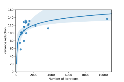
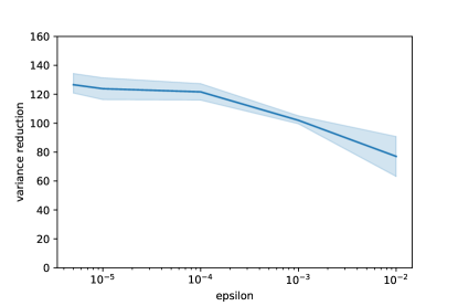
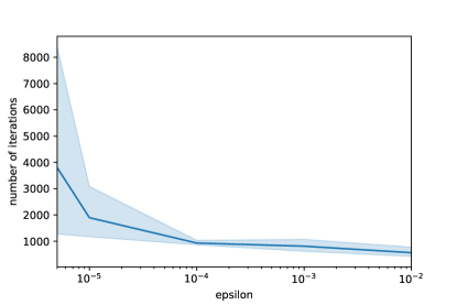
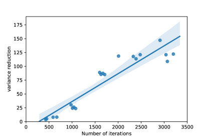
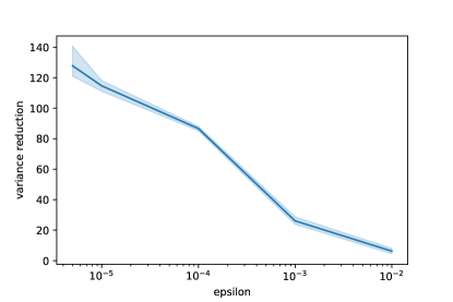
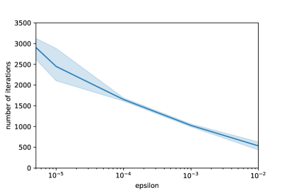
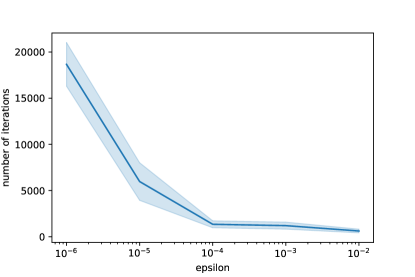
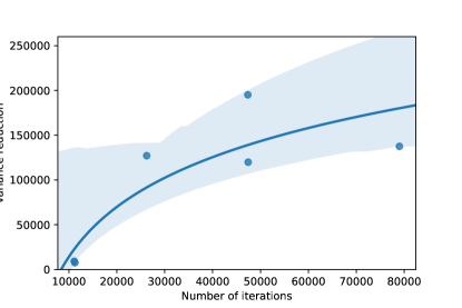
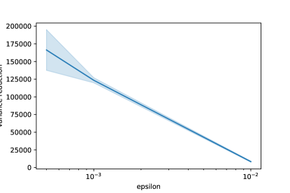
    Figure 2 studies the iterative training for the BSDE solver. As it has been observed before, this type of training does not allow us to study the overall loss function as the number of training steps increases. Therefore we train the same model four times for different values of ϵitalic-ϵ\epsilon between 0.010.010.01 and 5×1065superscript1065\times 10^{-6} and we study the number of iterations necessary to meet the stopping criteria defined by ϵitalic-ϵ\epsilon, the variance reduction once the stopping criteria is met, and the relationship between the number of iterations and the variance reduction. Note that the variance reduction stabilises for ϵ<105italic-ϵsuperscript105\epsilon<10^{-5}. Moreover, the number of iterations necessary to meet the stopping criteria increases exponentially as ϵitalic-ϵ\epsilon decreases, and therefore for our results printed in Tables 1 and 2 we employ ϵ=5×10⁶italic-ϵ5superscript106\epsilon=5\times 10^{-6}.

  4. iv)

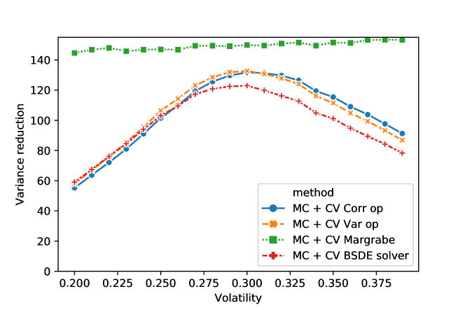
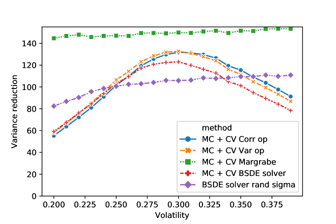
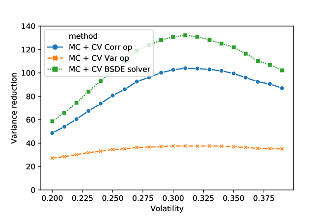
    Figure 4 displays the variance reduction after using the trained models on several Black Scholes problem with exchange options but with values of σ𝜎\sigma other than 0.30.30.3 which was the one used for training. We see that the various algorithms work similarly well in this case (not taking training cost into account). We note that the variance reduction is close to the theoretical maximum which is restricted by time discretisation. Finally we see that the variance reduction is still significant even when the neural network was trained with different model parameter (in our case volatility in the option pricing example). The labels of Figure 4 can be read as follows:

    1. i)

      MC + CV Corr op: Monte-Carlo estimate with Deep Learning-based Control Variate built using Algorithm 5.

    2. ii)

      MC + CV Var op: Monte-Carlo estimate with Deep Learning-based Control Variate built using Algorithm 4.

    3. iii)

      MC + CV BSDE solver: Monte-Carlo estimate with Deep Learning-based Control Variate built using Algorithm 3.

    4. iv)

      MC + CV Margrabe: Monte-Carlo estimate with Control Variate using analytical solution for this problem given by Margrabe formula.

Method Emp. Var. Var. Red. Fact. Train. Paths Opt. Steps
Monte Carlo 3.16×1023.16superscript1023.16\times 10^{-2} - - -
Algorithm 2 2.47×1042.47superscript1042.47\times 10^{-4} 127.7127.7127.7 38×10638superscript10638\times 10^{6} 7 60076007\,600
Algorithm 3 2.59×1042.59superscript1042.59\times 10^{-4} 121.98121.98121.98 6.945×1066.945superscript1066.945\times 10^{6} 138013801380
Algorithm 4 2.39×1042.39superscript1042.39\times 10^{-4} 132.28132.28132.28 36.055×10636.055superscript10636.055\times 10^{6} 721172117211
Algorithm 5 2.40×1042.40superscript1042.40\times 10^{-4} 131.53131.53131.53 45.61×10645.61superscript10645.61\times 10^{6} 912291229122
MC + CV Margrabe 2.12×1042.12superscript1042.12\times 10^{-4} 149.19149.19149.19 - -
MC + CV DGM [47] 1.22×1031.22superscript1031.22\times 10^{-3} 25.825.825.8 - -
Table 1. Results on exchange option problem on two assets, Example 4.1. Empirical Variance and variance reduction factor

Method Confidence Interval Variance Confidence Interval Estimator Monte Carlo [2.36×106,4.15×106]2.36superscript1064.15superscript106[2.36\times 10^{-6},4.15\times 10^{-6}] [0.1187,0.1195]0.11870.1195[0.1187,0.1195] Monte Carlo + antithetic paths [1.15×106,2.02×106]1.15superscript1062.02superscript106[1.15\times 10^{-6},2.02\times 10^{-6}] [0.1191,0.1195]0.11910.1195[0.1191,0.1195] Algorithm 2 [4.13×109,1.09×108]4.13superscript1091.09superscript108[4.13\times 10^{-9},1.09\times 10^{-8}] [0.11919,0.11926]0.119190.11926[0.11919,0.11926] Algorithm 3 [4.12×109,1.09×108]4.12superscript1091.09superscript108[4.12\times 10^{-9},1.09\times 10^{-8}] [0.11919,0.11925]0.119190.11925[0.11919,0.11925] Algorithm 4 [4.32×109,1.14×108]4.32superscript1091.14superscript108[4.32\times 10^{-9},1.14\times 10^{-8}] [0.11919,0.11926]0.119190.11926[0.11919,0.11926] Algorithm 5 [2.30×109,6.12×108]2.30superscript1096.12superscript108[2.30\times 10^{-9},6.12\times 10^{-8}] [0.11920,0.11924]0.119200.11924[0.11920,0.11924] MC + CV Margrabe [3.10×109,8.23×109]3.10superscript1098.23superscript109[3.10\times 10^{-9},8.23\times 10^{-9}] [0.11919,0.11925]0.119190.11925[0.11919,0.11925] MC + CV DGM [47] [3.10×109,8.23×109]3.10superscript1098.23superscript109[3.10\times 10^{-9},8.23\times 10^{-9}] [0.11919,0.11925]0.119190.11925[0.11919,0.11925]

Table 2. Results on exchange option problem on two assets, Example 4.1.
Refer to caption
Refer to caption
Figure 2. Left: Variance reduction in terms of number of optimiser iterations. Right: Variance reduction in terms of epsilon. Both are for Example 4.1 and Algorithm 3.
Refer to caption
Figure 3. Number of optimiser iterations in terms of epsilon for Example 4.1 and Algorithm 3.
Refer to caption
Figure 4. Variance reduction achieved by network trained with σ=0.3𝜎0.3\sigma=0.3 but then applied in situations where σ[0.2,0.4]𝜎0.20.4\sigma\in[0.2,0.4]. We can see that the significant variance reduction is achieved by a neural network that was trained with “incorrect” σ𝜎\sigma. Note that the “MC + CV Margbrabe” displays the optimal variance reduction that can be achieved by using exact solution to the problem. The variance reduction is not infinite even in this case since stochastic integrals are approximated by Riemann sums.
Example 4.2 (Low-dimensional problem with explicit solution - Approximation of Price using PDE solver compared to Control Variate).

We consider exchange options on two assets as in Example 4.1. We consider algorithm 3 that can be applied in two different ways:

  1. i)

    It directly approximates the solution of the PDE (5) and its gradient in every point.

  2. ii)

    We can use xvsubscript𝑥𝑣\partial_{x}v to build the control variate using probabilistic representation of the PDE  (6)

We compare both applications by calculating the expected error of the L2superscript𝐿2L^{2}-error of each of them with respect to the analytical solution given by Margrabe formula. From Margrabe’s formula we know that

v(0,S)=BlackScholes(risky price=S(1)S(2),strike=1,T,r,σ¯),𝑣0𝑆BlackScholesformulae-sequencerisky pricesuperscript𝑆1superscript𝑆2strike1𝑇𝑟¯𝜎v(0,S)=\text{BlackScholes}\left(\text{risky price}=\frac{S^{(1)}}{S^{(2)}},\text{strike}=1,T,r,\bar{\sigma}\right)\,,

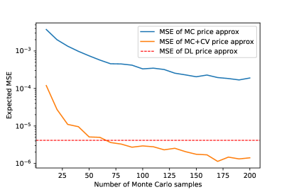
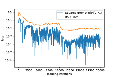
Let [v]η0(x)v(0,x)subscriptdelimited-[]𝑣subscript𝜂0𝑥𝑣0𝑥\mathcal{R}[v]_{\eta_{0}}(x)\approx v(0,x) be the Deep Learning approximation of price at any point at initial time, calculated using Algorithm 3, and [xv]θm(x)xv(tm,x)subscriptdelimited-[]subscript𝑥𝑣subscript𝜃𝑚𝑥subscript𝑥𝑣subscript𝑡𝑚𝑥\mathcal{R}[\partial_{x}v]_{\theta_{m}}(x)\approx\partial_{x}v(t_{m},x) be the Deep Learning approximation of its gradient for every time step in the time discretisation. The aim of this experiment is to show how even if Algorithm  3 numerically converges to a biased approximation of v(0,x)𝑣0𝑥v(0,x) (see Figure 5 left), it is still possible to use [xv]θm(x)subscriptdelimited-[]subscript𝑥𝑣subscript𝜃𝑚𝑥\mathcal{R}[\partial_{x}v]_{\theta_{m}}(x) to build an unbiased Monte-Carlo approximation of v(0,x)𝑣0𝑥v(0,x) with low variance.

We organise the experiment as follows.

  1. i)

    We calculate the expected value of the L2superscript𝐿2L^{2}-error of η0(x)subscript𝜂0𝑥\mathcal{R}\eta_{0}(x) where each component of x2𝑥superscript2x\in\mathbb{R}^{2} is sampled from a lognormal distribution:

    𝔼[|v(0,x)[v]η0(x)|2]1Ni=1N|v(0,xi)[v]η0(xi)|2𝔼delimited-[]superscript𝑣0𝑥subscriptdelimited-[]𝑣subscript𝜂0𝑥21𝑁superscriptsubscript𝑖1𝑁superscript𝑣0superscript𝑥𝑖subscriptdelimited-[]𝑣subscript𝜂0superscript𝑥𝑖2\mathbb{E}[|v(0,x)-\mathcal{R}[v]_{\eta_{0}}(x)|^{2}]\approx\frac{1}{N}\sum_{i=1}^{N}|v(0,x^{i})-\mathcal{R}[v]_{\eta_{0}}(x^{i})|^{2}
  2. ii)

    We calculate the expected value of the L2superscript𝐿2L^{2}-error of the Monte-Carlo estimator with control variate where each component of x2𝑥superscript2x\in\mathbb{R}^{2} is sampled from a lognormal distribution:

    𝔼[|v(0,x)𝒱0,Tπ,θ,λ,NMC,x|2]1Ni=1N|v(0,xi)𝒱0,Tπ,θ,λ,NMC,xi|2,𝔼delimited-[]superscript𝑣0𝑥subscriptsuperscript𝒱𝜋𝜃𝜆subscript𝑁𝑀𝐶𝑥0𝑇21𝑁superscriptsubscript𝑖1𝑁superscript𝑣0superscript𝑥𝑖subscriptsuperscript𝒱𝜋𝜃𝜆subscript𝑁𝑀𝐶superscript𝑥𝑖0𝑇2\mathbb{E}[|v(0,x)-\mathcal{V}^{\pi,\theta,\lambda,N_{MC},x}_{0,T}|^{2}]\approx\frac{1}{N}\sum_{i=1}^{N}|v(0,x^{i})-\mathcal{V}^{\pi,\theta,\lambda,N_{MC},x^{i}}_{0,T}|^{2}\,,

    where 𝒱0,Tπ,θ,λ,NMC,xsubscriptsuperscript𝒱𝜋𝜃𝜆subscript𝑁𝑀𝐶𝑥0𝑇\mathcal{V}^{\pi,\theta,\lambda,N_{MC},x}_{0,T} is given by 9, and is calculated for different values of Monte Carlo samples.

  3. iii)

    We calculate the expected value of the L2superscript𝐿2L^{2}-error of the Monte-Carlo estimator without control variate where each component of x2𝑥superscript2x\in\mathbb{R}^{2} is sampled from a lognormal distribution:

    𝔼[|v(0,x)Ξ0,Tπ,θ,λ,NMC,x|2]1Ni=1N|v(0,xi)Ξ0,Tπ,θ,λ,NMC,xi|2,𝔼delimited-[]superscript𝑣0𝑥subscriptsuperscriptΞ𝜋𝜃𝜆subscript𝑁𝑀𝐶𝑥0𝑇21𝑁superscriptsubscript𝑖1𝑁superscript𝑣0superscript𝑥𝑖subscriptsuperscriptΞ𝜋𝜃𝜆subscript𝑁𝑀𝐶superscript𝑥𝑖0𝑇2\mathbb{E}[|v(0,x)-\Xi^{\pi,\theta,\lambda,N_{MC},x}_{0,T}|^{2}]\approx\frac{1}{N}\sum_{i=1}^{N}|v(0,x^{i})-\Xi^{\pi,\theta,\lambda,N_{MC},x^{i}}_{0,T}|^{2}\,,

    where

    Ξ0,Tπ,θ,λ,NMC,x:=1NMCj=1NMCD(t,T)g(XTi)assignsubscriptsuperscriptΞ𝜋𝜃𝜆subscript𝑁𝑀𝐶𝑥0𝑇1subscript𝑁𝑀𝐶superscriptsubscript𝑗1subscript𝑁𝑀𝐶𝐷𝑡𝑇𝑔superscriptsubscript𝑋𝑇𝑖\Xi^{\pi,\theta,\lambda,N_{MC},x}_{0,T}:=\frac{1}{N_{MC}}\sum_{j=1}^{N_{MC}}D(t,T)g(X_{T}^{i})

Figure 5 provides one realisation of the described experiment for different Monte-Carlo iterations between 10 and 200. It shows how in this realisation, 60 Monte-Carlo iterations are enough to build a Monte-Carlo estimator with control variate having lower bias than the solution provided by Algorithm 3.
Refer to caption
Refer to caption
Figure 5. Left: Loss of Algorithm 3 and squared error of [v](t,x0)delimited-[]𝑣𝑡subscript𝑥0\mathcal{R}[v](t,x_{0}) in terms of training iterations. Right: Expected MSE of the two different approaches with respect to analytical solution in terms of number of Monte Carlo samples
Example 4.3 (Low-dimensional problem with explicit solution. Training on random values for volatility).

We consider exchange option on two assets. In this case the exact price is given by the Margrabe formula. The difference with respect to the last example is that now we aim to generalise our model, so that it can build control variates for different Black-Scholes models. For this we take d=2𝑑2d=2, S0i=100subscriptsuperscript𝑆𝑖0100S^{i}_{0}=100, r=0.05𝑟0.05r=0.05, σiUnif(0.2,0.4)similar-tosuperscript𝜎𝑖Unif0.20.4\sigma^{i}\sim\text{Unif}(0.2,0.4), Σii=1superscriptΣ𝑖𝑖1\Sigma^{ii}=1, Σij=0superscriptΣ𝑖𝑗0\Sigma^{ij}=0 for ij𝑖𝑗i\neq j.

The payoff is

g(S)=g(S(1),S(2)):=max(0,S(1)S(2)).𝑔𝑆𝑔superscript𝑆1superscript𝑆2assign0superscript𝑆1superscript𝑆2g(S)=g(S^{(1)},S^{(2)}):=\max\left(0,S^{(1)}-S^{(2)}\right)\,.

We organise the experiment as follows: for comparison purposes with the BSDE solver from the previous example, we train our model for exactly the same number of iterations, i.e. 1,38013801,380 batches of 5,000 random paths (stni)n=0Nstepssuperscriptsubscriptsuperscriptsubscript𝑠subscript𝑡𝑛𝑖𝑛0subscript𝑁steps(s_{t_{n}}^{i})_{n=0}^{N_{\text{steps}}} sampled from the SDE 12, where Nsteps=50subscript𝑁steps50N_{\text{steps}}=50. The assets’ initial values st0isuperscriptsubscript𝑠subscript𝑡0𝑖s_{t_{0}}^{i} are sampled from a lognormal distribution

Xexp((μ0.5σ2)τ+στξ),similar-to𝑋𝜇0.5superscript𝜎2𝜏𝜎𝜏𝜉X\sim\exp((\mu-0.5\sigma^{2})\tau+\sigma\sqrt{\tau}\xi),

where ξ𝒩(0,1),μ=0.08,τ=0.1formulae-sequencesimilar-to𝜉𝒩01formulae-sequence𝜇0.08𝜏0.1\xi\sim\mathcal{N}(0,1),\mu=0.08,\tau=0.1. Since now σ𝜎\sigma can take different values, it is included as input to the networks at each time step.

The existence of an explicit solution allows to build a control variate of the form (9) using the known exact solution to obtain xvsubscript𝑥𝑣\partial_{x}v. For a fixed number of time steps Nstepssubscript𝑁stepsN_{\text{steps}} this provides an upper bound on the variance reduction an artificial neural network approximation of xvsubscript𝑥𝑣\partial_{x}v can achieve.

Figure 6 adds the performance of this model to Figure 4, where the variance reduction of the Control Variate is displayed for different values of the volatility between 0.20.20.2 and 0.40.40.4.

Refer to caption
Figure 6. Extension of Figure 4 with variance reduction achieved by training the model on different Black-Scholes models
Example 4.4 (High-dimensional problem, exchange against average).

We extend the previous example to 100 dimensions. This example is similar to EX10EsubscriptEX10𝐸\text{EX}_{10E} from [8]. We will take S0i=100subscriptsuperscript𝑆𝑖0100S^{i}_{0}=100, r=5%𝑟percent5r=5\%, σi=30%superscript𝜎𝑖percent30\sigma^{i}=30\%, Σii=1superscriptΣ𝑖𝑖1\Sigma^{ii}=1, Σij=0superscriptΣ𝑖𝑗0\Sigma^{ij}=0 for ij𝑖𝑗i\neq j.

We will take this to be

g(S):=max(0,S11d1i=2dSi).assign𝑔𝑆0superscript𝑆11𝑑1superscriptsubscript𝑖2𝑑superscript𝑆𝑖g(S):=\max\left(0,S^{1}-\frac{1}{d-1}\sum_{i=2}^{d}S^{i}\right)\,.

The experiment is organised as follows: we train our models with batches of 51035superscript1035\cdot 10^{3} random paths (stni)n=0Nstepssuperscriptsubscriptsuperscriptsubscript𝑠subscript𝑡𝑛𝑖𝑛0subscript𝑁steps(s_{t_{n}}^{i})_{n=0}^{N_{\text{steps}}} sampled from the SDE (12), where Nsteps=50subscript𝑁steps50N_{\text{steps}}=50. The assets’ initial values st0isuperscriptsubscript𝑠subscript𝑡0𝑖s_{t_{0}}^{i} are sampled from a lognormal distribution

Xexp((μ0.5σ2)τ+στξ),similar-to𝑋𝜇0.5superscript𝜎2𝜏𝜎𝜏𝜉X\sim\exp((\mu-0.5\sigma^{2})\tau+\sigma\sqrt{\tau}\xi),

where ξN(0,1)similar-to𝜉𝑁01\xi\sim N(0,1), μ=0.08𝜇0.08\mu=0.08, τ=0.1𝜏0.1\tau=0.1.

We follow the evaluation framework to evaluate the model, simulating NMCNinsubscript𝑁MCsubscript𝑁inN_{\text{MC}}\cdot N_{\text{in}} paths by simulating (12) with constant S0i=1subscriptsuperscript𝑆𝑖01S^{i}_{0}=1 for i=1,,100𝑖1100i=1,\ldots,100. We have the following results:

  1. i)

    Table 3 provides the empirical variances calculated over 106superscript10610^{6} generated Monte Carlo samples and their corresponding control variates. The variance reduction measure indicates the quality of each control variate method. Table 3 also provides the cost of training for each method, given by the number of optimiser iterations performed before hitting the stopping criteria with ϵ=5106italic-ϵ5superscript106\epsilon=5\cdot 10^{-6}. Algorithm 3 outperforms the other algorithms in terms of variance reduction factor. This is not surprising as Algorithm 3 explicitly learns the discretisation of the Martingale representation (equation (7)) from which the control variate arises.

  2. ii)

    Table 4 provides the confidence interval for the variance of the Monte Carlo estimator, and the Monte Carlo estimator with control variate assuming these are calculated on 106superscript10610^{6} random paths.

  3. iii)

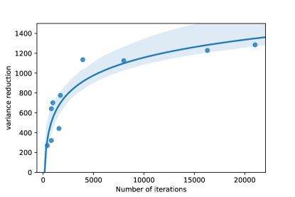
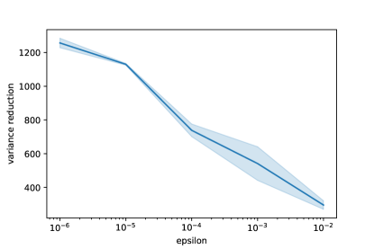
    Figures 7 and 8 study the iterative training for the BSDE solver. We train the same model four times for different values of ϵitalic-ϵ\epsilon between 0.010.010.01 and 5×1065superscript1065\times 10^{-6} and we study the number of iterations necessary to meet the stopping criteria defined by ϵitalic-ϵ\epsilon, the variance reduction once the stopping criteria is met, and the relationship between the number of iterations and the variance reduction. Note that in this case the variance reduction does not stabilise for ϵ<105italic-ϵsuperscript105\epsilon<10^{-5}. However, the number of training iterations increases exponentially as ϵitalic-ϵ\epsilon decreases, and therefore we also choose ϵ=5×10⁶italic-ϵ5superscript106\epsilon=5\times 10^{-6} to avoid building a control that requires a high number of random paths to be trained.

Method Emp. Var. Var. Red. Fact. Train. Paths Opt. Steps
Monte Carlo 1.97×1021.97superscript1021.97\times 10^{-2} - - -
Algorithm 2 5.94×1035.94superscript1035.94\times 10^{-3} 33.1633.1633.16 74×10674superscript10674\times 10^{6} 14 9001490014\,900
Algorithm 3 1.51×1041.51superscript1041.51\times 10^{-4} 130.39130.39130.39 14.145×10614.145superscript10614.145\times 10^{6} 2 82928292\,829
Algorithm 4 5.29×1045.29superscript1045.29\times 10^{-4} 37.2237.2237.22 97.265×10697.265superscript10697.265\times 10^{6} 19 4531945319\,453
Algorithm 5 1.93×1041.93superscript1041.93\times 10^{-4} 102.05102.05102.05 76.03×10676.03superscript10676.03\times 10^{6} 15 2061520615\,206
Table 3. Results on exchange option problem on 100 assets, Example 4.4. Empirical Variance and variance reduction factor and costs in terms of paths used for training and optimizer steps.

Method Confidence Interval Variance Confidence Interval Estimator Monte Carlo [1.51×106,2.65×106]1.51superscript1062.65superscript106[1.51\times 10^{-6},2.65\times 10^{-6}] [0.0845,0.0849]0.08450.0849[0.0845,0.0849] Monte Carlo + antithetic paths [8.77×107,1.53×106]8.77superscript1071.53superscript106[8.77\times 10^{-7},1.53\times 10^{-6}] [0.0845,0.0848]0.08450.0848[0.0845,0.0848] Algorithm 2 [3.04×108,2.14×107]3.04superscript1082.14superscript107[3.04\times 10^{-8},2.14\times 10^{-7}] [0.0848,0.08493]0.08480.08493[0.0848,0.08493] Algorithm 3 [5.32×109,1.41×108]5.32superscript1091.41superscript108[5.32\times 10^{-9},1.41\times 10^{-8}] [0.08485,0.8492]0.084850.8492[0.08485,0.8492] Algorithm 4 [4.13×109,1.09×108]4.13superscript1091.09superscript108[4.13\times 10^{-9},1.09\times 10^{-8}] [0.08484,0.08490]0.084840.08490[0.08484,0.08490] Algorithm 5 [3.80×109,1.0×108]3.80superscript1091.0superscript108[3.80\times 10^{-9},1.0\times 10^{-8}] [0.08487,0.08493]0.084870.08493[0.08487,0.08493]

Table 4. Results on exchange option problem on 100 assets, Example 4.4.
Refer to caption
Refer to caption
Figure 7. Left: Variance reduction in terms of number of optimiser iterations. Right: Variance reduction in terms of epsilon. Both for Example 4.4 and Algorithm 3.
Refer to caption
Figure 8. Number of optimiser iterations in terms of ϵitalic-ϵ\epsilon for Example 4.4 and Algorithm 3.
Refer to caption
Figure 9. Variance reduction with network trained with σ=0.3𝜎0.3\sigma=0.3 but applied for σ[0.2,0.4]𝜎0.20.4\sigma\in[0.2,0.4] for the model of Example 4.4. We see that the variance reduction factor is considerable even in the case when the network is used with “wrong” σ𝜎\sigma. It seems that Algorithm 4 is not performing well in this case.

Appendix A Martingale Control Variate

Let (Ω,,)Ω(\Omega,\mathcal{F},\mathbb{P}) be a probability space and consider an dsuperscriptsuperscript𝑑\mathbb{R}^{d^{\prime}}-valued Wiener process W=(Wj)j=1d=((Wtj)t0)j=1d𝑊superscriptsubscriptsuperscript𝑊𝑗𝑗1superscript𝑑superscriptsubscriptsubscriptsubscriptsuperscript𝑊𝑗𝑡𝑡0𝑗1superscript𝑑W=(W^{j})_{j=1}^{d^{\prime}}=((W^{j}_{t})_{t\geq 0})_{j=1}^{d^{\prime}}. We will use (tW)t0subscriptsubscriptsuperscript𝑊𝑡𝑡0(\mathcal{F}^{W}_{t})_{t\geq 0} to denote the filtration generated by W𝑊W. Consider a Dd𝐷superscript𝑑D\subseteq\mathbb{R}^{d}-valued, continuous, stochastic process defined for the parameters βBp𝛽𝐵superscript𝑝\beta\in B\subseteq\mathbb{R}^{p}, Xβ=(Xβ,i)i=1d=((Xtβ,i)t0)i=1dsuperscript𝑋𝛽superscriptsubscriptsuperscript𝑋𝛽𝑖𝑖1𝑑superscriptsubscriptsubscriptsubscriptsuperscript𝑋𝛽𝑖𝑡𝑡0𝑖1𝑑X^{\beta}=(X^{\beta,i})_{i=1}^{d}=((X^{\beta,i}_{t})_{t\geq 0})_{i=1}^{d} adapted to (tW)t0subscriptsubscriptsuperscript𝑊𝑡𝑡0(\mathcal{F}^{W}_{t})_{t\geq 0}.

Let g:C([0,T],d):𝑔𝐶0𝑇superscript𝑑g:C([0,T],\mathbb{R}^{d})\to\mathbb{R} be a measurable function. We shall consider path-dependent contingent claims of the form g((Xsβ)s[0,T])𝑔subscriptsuperscriptsubscript𝑋𝑠𝛽𝑠0𝑇g((X_{s}^{\beta})_{s\in[0,T]}). Finally we assume that there is a (stochastic) discount factor given by

D(t1,t2;β)=et1t2c(s,Xsβ;β)𝑑s𝐷subscript𝑡1subscript𝑡2𝛽superscript𝑒superscriptsubscriptsubscript𝑡1subscript𝑡2𝑐𝑠superscriptsubscript𝑋𝑠𝛽𝛽differential-d𝑠D(t_{1},t_{2};\beta)=e^{-\int_{t_{1}}^{t_{2}}c(s,X_{s}^{\beta};\beta)ds}

for an appropriate function c=c(t,x;β)𝑐𝑐𝑡𝑥𝛽c=c(t,x;\beta). We will omit the β𝛽\beta from the discount factor notation. Let

ΞTβ:=D(t,T)g((Xsβ)s[0,T]).assignsuperscriptsubscriptΞ𝑇𝛽𝐷𝑡𝑇𝑔subscriptsuperscriptsubscript𝑋𝑠𝛽𝑠0𝑇\Xi_{T}^{\beta}:=D(t,T)g((X_{s}^{\beta})_{s\in[0,T]})\,.

We now interpret \mathbb{P} as some risk-neutral measure and so the \mathbb{P}-price of our contingent claim is

Vtβ=𝔼[ΞTβ|tβ]=𝔼[D(t,T)g((Xsβ)s[0,T])|tβ].superscriptsubscript𝑉𝑡𝛽𝔼delimited-[]conditionalsuperscriptsubscriptΞ𝑇𝛽superscriptsubscript𝑡𝛽𝔼delimited-[]conditional𝐷𝑡𝑇𝑔subscriptsuperscriptsubscript𝑋𝑠𝛽𝑠0𝑇superscriptsubscript𝑡𝛽V_{t}^{\beta}=\mathbb{E}\left[\Xi_{T}^{\beta}\big{|}\mathcal{F}_{t}^{\beta}\right]=\mathbb{E}\left[D(t,T)g((X_{s}^{\beta})_{s\in[0,T]})\big{|}\mathcal{F}_{t}^{\beta}\right]\,.

By assumption ΞTβsuperscriptsubscriptΞ𝑇𝛽\Xi_{T}^{\beta} is TWsuperscriptsubscript𝑇𝑊\mathcal{F}_{T}^{W} measurable and 𝔼[|ΞTβ|2]<𝔼delimited-[]superscriptsuperscriptsubscriptΞ𝑇𝛽2\mathbb{E}[|\Xi_{T}^{\beta}|^{2}]<\infty. Hence, from the Martingale Representation Theorem, see e.g. [11, Th. 14.5.1], there exists a unique process (Ztβ)tsubscriptsuperscriptsubscript𝑍𝑡𝛽𝑡(Z_{t}^{\beta})_{t} adapted to (tW)tsubscriptsuperscriptsubscript𝑡𝑊𝑡(\mathcal{F}_{t}^{W})_{t} with 𝔼[0T|Zsβ|2𝑑s]<𝔼delimited-[]superscriptsubscript0𝑇superscriptsuperscriptsubscript𝑍𝑠𝛽2differential-d𝑠\mathbb{E}[\int_{0}^{T}|Z_{s}^{\beta}|^{2}ds]<\infty such that

ΞTβ=𝔼[ΞTβ|0W]+0TZsβ𝑑Ws.superscriptsubscriptΞ𝑇𝛽𝔼delimited-[]conditionalsuperscriptsubscriptΞ𝑇𝛽subscriptsuperscript𝑊0superscriptsubscript0𝑇superscriptsubscript𝑍𝑠𝛽differential-dsubscript𝑊𝑠\Xi_{T}^{\beta}=\mathbb{E}[\Xi_{T}^{\beta}\big{|}\mathcal{F}^{W}_{0}]+\int_{0}^{T}Z_{s}^{\beta}\,dW_{s}\,. (13)

The proof of the existence of the process (Ztβ)tsubscriptsuperscriptsubscript𝑍𝑡𝛽𝑡(Z_{t}^{\beta})_{t}, is non-constructive. In the setup of the paper, we used the Markovian property of ΞtβsuperscriptsubscriptΞ𝑡𝛽\Xi_{t}^{\beta} to approximate Ztβsuperscriptsubscript𝑍𝑡𝛽Z_{t}^{\beta} via the associated linear PDE. In the more general non-Markovian setup, [12] provides a numerical method to construct the martingale representation.

Observe that in our setup, 0=0Wsubscript0superscriptsubscript0𝑊\mathcal{F}_{0}=\mathcal{F}_{0}^{W}, tβtWsuperscriptsubscript𝑡𝛽superscriptsubscript𝑡𝑊\mathcal{F}_{t}^{\beta}\subseteq\mathcal{F}_{t}^{W} for t0𝑡0t\geq 0. Hence tower property of the conditional expectation implies that

𝔼[ΞTβ|tβ]=𝔼[ΞTβ|0W]+0tZsβ𝑑Ws.𝔼delimited-[]conditionalsuperscriptsubscriptΞ𝑇𝛽superscriptsubscript𝑡𝛽𝔼delimited-[]conditionalsuperscriptsubscriptΞ𝑇𝛽subscriptsuperscript𝑊0superscriptsubscript0𝑡superscriptsubscript𝑍𝑠𝛽differential-dsubscript𝑊𝑠\mathbb{E}[\Xi_{T}^{\beta}\big{|}\mathcal{F}_{t}^{\beta}]=\mathbb{E}[\Xi_{T}^{\beta}\big{|}\mathcal{F}^{W}_{0}]+\int_{0}^{t}Z_{s}^{\beta}\,dW_{s}\,. (14)

Consequently (13) and (14) imply

𝔼[ΞTβ|tβ]=ΞTβtTZsβ𝑑Ws.𝔼delimited-[]conditionalsuperscriptsubscriptΞ𝑇𝛽superscriptsubscript𝑡𝛽superscriptsubscriptΞ𝑇𝛽superscriptsubscript𝑡𝑇superscriptsubscript𝑍𝑠𝛽differential-dsubscript𝑊𝑠\mathbb{E}[\Xi_{T}^{\beta}\big{|}\mathcal{F}_{t}^{\beta}]=\Xi_{T}^{\beta}-\int_{t}^{T}Z_{s}^{\beta}\,dW_{s}\,.

We then observe that

Vtβ=𝔼[ΞTβ|tβ]=𝔼[ΞTβtTZsβ𝑑Ws|tβ].superscriptsubscript𝑉𝑡𝛽𝔼delimited-[]conditionalsuperscriptsubscriptΞ𝑇𝛽superscriptsubscript𝑡𝛽𝔼delimited-[]superscriptsubscriptΞ𝑇𝛽conditionalsuperscriptsubscript𝑡𝑇superscriptsubscript𝑍𝑠𝛽differential-dsubscript𝑊𝑠superscriptsubscript𝑡𝛽V_{t}^{\beta}=\mathbb{E}[\Xi_{T}^{\beta}\big{|}\mathcal{F}_{t}^{\beta}]=\mathbb{E}\left[\Xi_{T}^{\beta}-\int_{t}^{T}Z_{s}^{\beta}\,dW_{s}\bigg{|}\mathcal{F}_{t}^{\beta}\right]\,.

If we can generate iid (Wi)i=1Nsuperscriptsubscriptsuperscript𝑊𝑖𝑖1𝑁(W^{i})_{i=1}^{N} and (Zβ,i)i=1Nsuperscriptsubscriptsuperscript𝑍𝛽𝑖𝑖1𝑁(Z^{\beta,i})_{i=1}^{N} with the same distributions as W𝑊W and Z𝑍Z respectively then we can consider the following Monte-Carlo estimator of Vtβsuperscriptsubscript𝑉𝑡𝛽V_{t}^{\beta}:

𝒱tβ,N:=1Ni=1N(ΞTβ,itTZsβ,i𝑑Wsi).assignsubscriptsuperscript𝒱𝛽𝑁𝑡1𝑁superscriptsubscript𝑖1𝑁superscriptsubscriptΞ𝑇𝛽𝑖superscriptsubscript𝑡𝑇subscriptsuperscript𝑍𝛽𝑖𝑠differential-dsubscriptsuperscript𝑊𝑖𝑠\mathcal{V}^{\beta,N}_{t}:=\frac{1}{N}\sum_{i=1}^{N}\left(\Xi_{T}^{\beta,i}-\int_{t}^{T}Z^{\beta,i}_{s}\,dW^{i}_{s}\right)\,.

In the companion paper [45] we provide deep learning algorithms to price path-dependent options in the risk neutral measure by solving the corresponding path-dependent PDE, using a combination of Recurrent Neural networks and path signatures to parametrise the process Zβsuperscript𝑍𝛽Z^{\beta}.

Appendix B Martingale Control Variate Deep Solvers

B.1. Empirical correlation maximisation

This method is based on the idea that since we are looking for a good control variate we should directly train the network to maximise the variance reduction between the vanilla Monte-Carlo estimator and the control variates Monte-Carlo estimator by also trying to optimise λ𝜆\lambda.

Recall we denote ΞT=D(t,T)g((Xs)s[t,T])subscriptΞ𝑇𝐷𝑡𝑇𝑔subscriptsubscript𝑋𝑠𝑠𝑡𝑇\Xi_{T}=D(t,T)g((X_{s})_{s\in[t,T]}). We also denote as Mt,Tsubscript𝑀𝑡𝑇M_{t,T} as the stochastic integral that arises in the martingale representation of ΞTsubscriptΞ𝑇\Xi_{T}. The optimal coefficient λ,θsuperscript𝜆𝜃\lambda^{*,\theta} that minimises the variance 𝕍ar[ΞTλMt,Tθ]𝕍ardelimited-[]subscriptΞ𝑇𝜆subscriptsuperscript𝑀𝜃𝑡𝑇\mathbb{V}\text{ar}[\Xi_{T}-\lambda M^{\theta}_{t,T}] is

λ,θ=ov[ΞT,Mt,Tθ]𝕍ar[Mt,Tθ].superscript𝜆𝜃ovsubscriptΞ𝑇subscriptsuperscript𝑀𝜃𝑡𝑇𝕍ardelimited-[]subscriptsuperscript𝑀𝜃𝑡𝑇\lambda^{*,\theta}=\frac{\mathbb{C}\text{ov}[\Xi_{T},M^{\theta}_{t,T}]}{\mathbb{V}\text{ar}[M^{\theta}_{t,T}]}\,.

Let ρΞT,Mt,Tθsuperscript𝜌subscriptΞ𝑇subscriptsuperscript𝑀𝜃𝑡𝑇\rho^{\Xi_{T},M^{\theta}_{t,T}} denote the Pearson correlation coefficient between ΞTsubscriptΞ𝑇\Xi_{T} and Mt,Tθsubscriptsuperscript𝑀𝜃𝑡𝑇M^{\theta}_{t,T} i.e.

ρΞT,Mt,Tθ=ov(ΞT,Mt,Tθ)𝕍ar[ΞT]𝕍ar[Mt,Tθ].superscript𝜌subscriptΞ𝑇subscriptsuperscript𝑀𝜃𝑡𝑇ovsubscriptΞ𝑇subscriptsuperscript𝑀𝜃𝑡𝑇𝕍ardelimited-[]subscriptΞ𝑇𝕍ardelimited-[]subscriptsuperscript𝑀𝜃𝑡𝑇\rho^{\Xi_{T},M^{\theta}_{t,T}}=\frac{\mathbb{C}\text{ov}(\Xi_{T},M^{\theta}_{t,T})}{\sqrt{\mathbb{V}\text{ar}[\Xi_{T}]\mathbb{V}\text{ar}[M^{\theta}_{t,T}]}}\,.

With the optimal λsuperscript𝜆\lambda^{*} we then have that the variance reduction obtained from the control variate is

𝕍ar[𝒱t,Tπ,θ,λ,N]𝕍ar[ΞT]=1(ρΞT,Mt,Tθ)2.𝕍ardelimited-[]subscriptsuperscript𝒱𝜋𝜃superscript𝜆𝑁𝑡𝑇𝕍ardelimited-[]subscriptΞ𝑇1superscriptsuperscript𝜌subscriptΞ𝑇subscriptsuperscript𝑀𝜃𝑡𝑇2\frac{\mathbb{V}\text{ar}[\mathcal{V}^{\pi,\theta,\lambda^{*},N}_{t,T}]}{\mathbb{V}\text{ar}[\Xi_{T}]}=1-\bigg{(}\rho^{\Xi_{T},M^{\theta}_{t,T}}\bigg{)}^{2}\,.

See [17, Ch. 4.1] for more details. Therefore we set the learning task as:

θ,cor:=argminθ[1(ρΞT,Mt,Tθ)2].assignsuperscript𝜃𝑐𝑜𝑟subscriptargmin𝜃1superscriptsuperscript𝜌subscriptΞ𝑇subscriptsuperscript𝑀𝜃𝑡𝑇2\theta^{*,cor}:=\operatorname*{arg\,min}_{\theta}\left[1-\bigg{(}\rho^{\Xi_{T},M^{\theta}_{t,T}}\bigg{)}^{2}\ \right]\,.

The implementable version requires the definition of 𝒱t,Tβ,π,θ,λ,Nsubscriptsuperscript𝒱𝛽𝜋𝜃𝜆𝑁𝑡𝑇\mathcal{V}^{\beta,\pi,\theta,\lambda,N}_{t,T} in (9), where we set

ΞTβ,π,i:=Dπ(t,T))ig(XTβ,π,i)Mt,Tβ,π,i,θ:=k=1Nsteps1(Dπ(t,tk))i[xv]θ(tk,Xtkβ,π,i)σ(tk,Xtkβ,π,i)(Wtk+1iWtki)\begin{split}\Xi_{T}^{\beta,\pi,i}:=&D^{\pi}(t,T))^{i}g(X^{\beta,\pi,i}_{T})\\ M_{t,T}^{\beta,\pi,i,\theta}:=&\sum_{k=1}^{N_{\text{steps}}-1}(D^{\pi}(t,t_{k}))^{i}\mathcal{R}[\partial_{x}v]_{\theta}(t_{k},X^{\beta,\pi,i}_{t_{k}})\sigma(t_{k},X^{\beta,\pi,i}_{t_{k}})\,(W^{i}_{t_{k+1}}-W^{i}_{t_{k}})\end{split}

The full method is stated as Algorithm 5.

Algorithm 5 Martingale control variates solver: Empirical correlation maximization
  Initialisation: θ𝜃\theta, Ntrnsubscript𝑁trnN_{\text{trn}}
  for i:1:Ntrn:𝑖1:subscript𝑁trni:1:N_{\text{trn}} do
      generate samples (xtβ,π,i)tπsubscriptsuperscriptsubscript𝑥𝑡𝛽𝜋𝑖𝑡𝜋(x_{t}^{\beta,\pi,i})_{t\in\pi} by using numerical SDE solver on (2) and sampling from the distribution of β𝛽\beta.
  end for
  Find θ,Ntrnsuperscript𝜃subscript𝑁trn\theta^{*,N_{\text{trn}}} using SGD where
θ,Ntrn:=argminθ[1(ovNtrn(ΞTβ,π)𝕍arNtrn[ΞTβ,π]𝕍arNtrn[Mt,Tβ,π,θ])2],assignsuperscript𝜃subscript𝑁trnsubscriptargmin𝜃1superscriptsuperscriptovsubscript𝑁trnsuperscriptsubscriptΞ𝑇𝛽𝜋𝕍superscriptarsubscript𝑁trndelimited-[]superscriptsubscriptΞ𝑇𝛽𝜋𝕍superscriptarsubscript𝑁trndelimited-[]subscriptsuperscript𝑀𝛽𝜋𝜃𝑡𝑇2\begin{split}\theta^{*,N_{\text{trn}}}:=&\operatorname*{arg\,min}_{\theta}\left[1-\left(\frac{\mathbb{C}\text{ov}^{N_{\text{trn}}}(\Xi_{T}^{\beta,\pi})}{\sqrt{\mathbb{V}\text{ar}^{N_{\text{trn}}}[\Xi_{T}^{\beta,\pi}]\mathbb{V}\text{ar}^{N_{\text{trn}}}[M^{\beta,\pi,\theta}_{t,T}]}}\right)^{2}\,\,\right]\,,\end{split}
where 𝕍arNtrn,ovNtrn𝕍superscriptarsubscript𝑁trnsuperscriptovsubscript𝑁trn\mathbb{V}\text{ar}^{N_{\text{trn}}},\mathbb{C}\text{ov}^{N_{\text{trn}}} denote the empirical variance and covariance.
  return  θ,Ntrnsuperscript𝜃subscript𝑁trn\theta^{*,N_{\text{trn}}}.

Appendix C Artificial neural networks

We fix a locally Lipschitz function 𝐚::𝐚\mathbf{a}:\mathbb{R}\to\mathbb{R} and for d𝑑d\in\mathbb{N} define 𝐀d:dd:subscript𝐀𝑑superscript𝑑superscript𝑑\mathbf{A}_{d}:\mathbb{R}^{d}\to\mathbb{R}^{d} as the function given, for x=(x1,,xd)𝑥subscript𝑥1subscript𝑥𝑑x=(x_{1},\ldots,x_{d}) by 𝐀d(x)=(𝐚(x1),,𝐚(xd))subscript𝐀𝑑𝑥𝐚subscript𝑥1𝐚subscript𝑥𝑑\mathbf{A}_{d}(x)=(\mathbf{a}(x_{1}),\ldots,\mathbf{a}(x_{d})). We fix L𝐿L\in\mathbb{N} (the number of layers), lksubscript𝑙𝑘l_{k}\in\mathbb{N}, k=0,1,L1𝑘01𝐿1k=0,1,\ldots L-1 (the size of input to layer k𝑘k) and lLsubscript𝑙𝐿l_{L}\in\mathbb{N} (the size of the network output). A fully connected artificial neural network is then given by Φ=((W1,B1),,(WL,BL))Φsubscript𝑊1subscript𝐵1subscript𝑊𝐿subscript𝐵𝐿\Phi=((W_{1},B_{1}),\ldots,(W_{L},B_{L})), where, for k=1,,L𝑘1𝐿k=1,\ldots,L, we have real lk1×lksubscript𝑙𝑘1subscript𝑙𝑘l_{k-1}\times l_{k} matrices Wksubscript𝑊𝑘W_{k} and real lksubscript𝑙𝑘l_{k} dimensional vectors Bksubscript𝐵𝑘B_{k}.

The artificial neural network defines a function Φ:l0lL:subscriptΦsuperscriptsubscript𝑙0superscriptsubscript𝑙𝐿\mathcal{R}_{\Phi}:\mathbb{R}^{l_{0}}\to\mathbb{R}^{l_{L}} given recursively, for x0l0subscript𝑥0superscriptsubscript𝑙0x_{0}\in\mathbb{R}^{l_{0}}, by

Φ(x0)=WLxL1+BL,xk=𝐀lk(Wkxk1+Bk),k=1,,L1.formulae-sequencesubscriptΦsubscript𝑥0subscript𝑊𝐿subscript𝑥𝐿1subscript𝐵𝐿formulae-sequencesubscript𝑥𝑘subscript𝐀subscript𝑙𝑘subscript𝑊𝑘subscript𝑥𝑘1subscript𝐵𝑘𝑘1𝐿1\mathcal{R}_{\Phi}(x_{0})=W_{L}x_{L-1}+B_{L}\,,\,\,\,\,x_{k}=\mathbf{A}_{l_{k}}(W_{k}x_{k-1}+B_{k})\,,k=1,\ldots,L-1\,.

We can also define the function 𝒫𝒫\mathcal{P} which counts the number of parameters as

𝒫(Φ)=i=1L(lk1lk+lk).𝒫Φsuperscriptsubscript𝑖1𝐿subscript𝑙𝑘1subscript𝑙𝑘subscript𝑙𝑘\mathcal{P}(\Phi)=\sum_{i=1}^{L}(l_{k-1}l_{k}+l_{k})\,.

We will call such class of fully connected artificial neural networks 𝒟𝒩𝒟𝒩\mathcal{DN}. Note that since the activation functions and architecture are fixed the learning task entails finding the optimal Φ𝒫(Φ)Φsuperscript𝒫Φ\Phi\in\mathbb{R}^{\mathcal{P}(\Phi)}.

Appendix D Additional numerical results

Example D.1 (Low dimensional basket option).

We consider the basket options problem of pricing, using the example from [5, Sec 4.2.3]. The payoff function is

g(S):=max(0,i=1dSiK).assign𝑔𝑆0superscriptsubscript𝑖1𝑑superscript𝑆𝑖𝐾g(S):=\max\left(0,\sum_{i=1}^{d}S^{i}-K\right)\,.

We first consider the basket options problem on two assets, with d=2𝑑2d=2, S0i=70subscriptsuperscript𝑆𝑖070S^{i}_{0}=70, r=50%𝑟percent50r=50\%, σi=100%superscript𝜎𝑖percent100\sigma^{i}=100\%, Σii=1superscriptΣ𝑖𝑖1\Sigma^{ii}=1, Σij=0superscriptΣ𝑖𝑗0\Sigma^{ij}=0 for ij𝑖𝑗i\neq j, and constant strike K=i=1dS0i𝐾superscriptsubscript𝑖1𝑑subscriptsuperscript𝑆𝑖0K=\sum_{i=1}^{d}S^{i}_{0}. In line with the example from [5, Sec 4.2.3] for comparison purposes we organise the experiment as follows. The control variates on 20 0002000020\,000 batches of 5 00050005\,000 samples each of (stni)n=0Nstepssuperscriptsubscriptsuperscriptsubscript𝑠subscript𝑡𝑛𝑖𝑛0subscript𝑁steps(s_{t_{n}}^{i})_{n=0}^{N_{\text{steps}}} by simulating the SDE 12, where Nsteps=50subscript𝑁steps50N_{\text{steps}}=50. The assets’ initial values st0subscript𝑠subscript𝑡0s_{t_{0}} are always constant St0i=0.7superscriptsubscript𝑆subscript𝑡0𝑖0.7S_{t_{0}}^{i}=0.7. We follow the evaluation framework to evaluate the model, simulating NMCNinsubscript𝑁MCsubscript𝑁inN_{\text{MC}}\cdot N_{\text{in}} paths by simulating 12 with constant S0i=0.7subscriptsuperscript𝑆𝑖00.7S^{i}_{0}=0.7 for i=1,,100𝑖1100i=1,\ldots,100. We have the following results:

  1. i)

    Table 5 provides the empirical variances calculated over 106superscript10610^{6} generated Monte Carlo samples and their corresponding control variates. The variance reduction measure indicates the quality of each control variate method. Table 5 also provides the cost of training for each method, given by the number of optimiser iterations performed before hitting the stopping criteria, defined defined before with ϵ=5×10⁶italic-ϵ5superscript106\epsilon=5\times 10^{-6}.

  2. ii)

    Table 6 provides the confidence interval for the variance of the Monte Carlo estimator, and the Monte Carlo estimator with control variate assuming these are calculated on 106superscript10610^{6} random paths.

  3. iii)

    Figures 10 and 11 study the iterative training for the BSDE solver. We train the same model four times for different values of ϵitalic-ϵ\epsilon between 0.010.010.01 and 5×1065superscript1065\times 10^{-6} and we study the number of iterations necessary to meet the stopping criteria defined by ϵitalic-ϵ\epsilon, the variance reduction once the stopping criteria is met, and the relationship between the number of iterations and the variance reduction. Note that the variance reduction stabilises for ϵ<105italic-ϵsuperscript105\epsilon<10^{-5}. Furthermore, the number of training iterations increases exponentially as ϵitalic-ϵ\epsilon decreases. We choose ϵ=5×10⁶italic-ϵ5superscript106\epsilon=5\times 10^{-6}.

We note that in the example from [5, Sec 4.2.3], the control variate is trained with S0=0.7subscript𝑆00.7S_{0}=0.7 fixed. Using this setting, Algorithm 2 cannot be used to approximate the control variate in (9): since the network at t=0𝑡0t=0, [v]η0subscriptdelimited-[]𝑣subscript𝜂0\mathcal{R}[v]_{\eta_{0}}, is trained only at S0=0.7subscript𝑆00.7S_{0}=0.7, then automatic differentiation to approximate x[v]η0(0.7)subscript𝑥subscriptdelimited-[]𝑣subscript𝜂00.7\partial_{x}\mathcal{R}[v]_{\eta_{0}}(0.7) will yield a bad approximation of xv(0.7)subscript𝑥𝑣0.7\partial_{x}v(0.7); indeed, during training [v]η0subscriptdelimited-[]𝑣subscript𝜂0\mathcal{R}[v]_{\eta_{0}} is unable to capture how v𝑣v changes around S0subscript𝑆0S_{0} at t=0𝑡0t=0. For this reason, Algorithm 2 is not included in the following results.

Method Emp. Var. Var. Red. Fact. Train. Paths Optimizer steps
Monte Carlo 1.391.391.39 - - -
Algorithm 3 1.13×1031.13superscript1031.13\times 10^{-3} 121912191219 8×1078superscript1078\times 10^{7} 16 1291612916\,129
Algorithm 4 1.13×1031.13superscript1031.13\times 10^{-3} 122812281228 3×1073superscript1073\times 10^{7} 6 60166016\,601
Algorithm 5 1.29×1031.29superscript1031.29\times 10^{-3} 107610761076 4×1074superscript1074\times 10^{7} 8 03580358\,035
Table 5. Results on basket options problem on two assets, Example D.1. Models trained with S0subscript𝑆0S_{0} fixed, non-random. Empirical Variance and variance reduction factor are presented.
Method Confidence Interval Variance Confidence Interval Estimator
Monte Carlo [4.49×105,1.19×104]4.49superscript1051.19superscript104[4.49\times 10^{-5},1.19\times 10^{-4}] [0.665,0.671]0.6650.671[0.665,0.671]
Monte Carlo + antithetic paths [1.43×105,2.51×105]1.43superscript1052.51superscript105[1.43\times 10^{-5},2.51\times 10^{-5}] [0.667,0.670]0.6670.670[0.667,0.670]
Algorithm 3 [2.1329×108,5.6610×108]2.1329superscript1085.6610superscript108[2.1329\times 10^{-8},5.6610\times 10^{-8}] [0.6696,0.6697]0.66960.6697[0.6696,0.6697]
Algorithm 4 [1.687×108,4.47×107]1.687superscript1084.47superscript107[1.687\times 10^{-8},4.47\times 10^{-7}] [0.6695,0.6697]0.66950.6697[0.6695,0.6697]
Algorithm 5 [1.746×108,4.63×108]1.746superscript1084.63superscript108[1.746\times 10^{-8},4.63\times 10^{-8}] [0.6695,0.6697]0.66950.6697[0.6695,0.6697]
Table 6. Results on basket options problem on two assets, Example D.1. Models trained with S0subscript𝑆0S_{0} fixed, non-random.
Refer to caption
Refer to caption
Figure 10. Left: Variance reduction in terms of number of optimiser iterations. Right: Variance reduction in terms of epsilon. Both refer to Algorithm 3 used in Example D.1.
Refer to caption
Figure 11. Number of optimiser iterations in terms of ϵitalic-ϵ\epsilon for Algorithm 3 used in Example D.1.
Example D.2 (basket option with random sigma).

In this example, as in Example 4.2, we aim to show how our approach - where we build a control variate by approximating the process (Ztk)k=0,,Nstepssubscriptsubscript𝑍subscript𝑡𝑘𝑘0subscript𝑁steps(Z_{t_{k}})_{k=0,\ldots,N_{\text{steps}}} - is more robust compared to directly approximating the price by a certain function in a high-dimensional setting.

We use the methodology proposed in [7], where the authors present a deep learning-based calibration method proposing a two-steps approach: first the authors learn the model that approximates the pricing map using a artificial neural network in which the inputs are the parameters of the volatility model. Second the authors calibrate the learned model using available data by means of different optimisation methods.

For a fair comparison between our deep learning based control variate approach vs. the method proposed in [7], we make the following remarks:

  1. i)

    We will only use the the first step detailed in [7] where the input to the model that approximates the pricing map are the volatility model’s parameters: σd,r𝜎superscript𝑑𝑟\sigma\in\mathbb{R}^{d},r, and the initial price is considered constant for training purposes. We run the experiment for d=5𝑑5d=5.

  2. ii)

    In [7] the authors build a training set, and then perform gradient descent-based optimisation on the training set for a number of epochs. This is somewhat a limiting factor in the current setting where one can have as much data as they want since it is generated from some given distributions. In line with our experiments, instead of building a training set, in each optimisation step we sample a batch from the given distributions.

  3. iii)

    In [7], the price mapping function is learned for a grid of combinations of maturities and strikes. In this experiment, we reduce the grid to just one point considering T=0.5𝑇0.5T=0.5, K=iS0i𝐾subscript𝑖superscriptsubscript𝑆0𝑖K=\sum_{i}S_{0}^{i}, where S0i=0.7isuperscriptsubscript𝑆0𝑖0.7for-all𝑖S_{0}^{i}=0.7\,\,\forall i.

  4. iv)

    We will use Algorithm 3 to build the control variate with the difference that now σd,rformulae-sequence𝜎superscript𝑑𝑟\sigma\in\mathbb{R}^{d},r\in\mathbb{R} will be passed as input to the each network at each time step [v]ηk,[xv]θksubscriptdelimited-[]𝑣subscript𝜂𝑘subscriptdelimited-[]subscript𝑥𝑣subscript𝜃𝑘\mathcal{R}[v]_{\eta_{k}},\mathcal{R}[\partial_{x}v]_{\theta_{k}}.

The experiment is organised as follows:

  1. i)

    We train the network proposed in [7] approximating the price using Black-Scholes model and Basket options payoff. In each optimisation iteration a batch of size 1 00010001\,000, where the volatility model’s parameters are sampled using σ𝒰(0.9,1.1)similar-to𝜎𝒰0.91.1\sigma\sim\mathcal{U}(0.9,1.1) and r𝒰(0.4,0.6)similar-to𝑟𝒰0.40.6r\sim\mathcal{U}(0.4,0.6). We keep a test set of size 150, 𝒮={[(σi,ri);p(σi,ri)],i=1,,150}\mathcal{S}=\{\left[(\sigma^{i},r^{i});p(\sigma^{i},r^{i})\right],i=1,\ldots,150\} where p(σi,ri)𝑝superscript𝜎𝑖superscript𝑟𝑖p(\sigma^{i},r^{i}) denotes the price and is generated using 50 0005000050\,000 Monte Carlo samples.

  2. ii)

    We use Algorithm 3 to build the control variate, where σ𝜎\sigma and r𝑟r are sampled as above and are included as inputs to the network. We denote the trained model by [xv]θksubscriptdelimited-[]subscript𝑥𝑣subscript𝜃𝑘\mathcal{R}[\partial_{x}v]_{\theta_{k}} where k=1,,Nsteps𝑘1subscript𝑁stepsk=1,\ldots,N_{\text{steps}}. In contrast with Algorithm 3.

We present the following results:

  1. i)

    Figure 1 displays the histogram of the squared error of the approximation of the PDE solution [v]ηsubscriptdelimited-[]𝑣𝜂\mathcal{R}[v]_{\eta} for each instance in 𝒮𝒮\mathcal{S}. In this sample, it spans from almost 108superscript10810^{-8} to 103superscript10310^{-}3, i.e. for almost five orders of magnitude.

  2. ii)

    We build the control variate for that instance in the test set for which [v]ηsubscriptdelimited-[]𝑣𝜂\mathcal{R}[v]_{\eta} generalises the worst. For those particular σ,r𝜎𝑟\sigma,r, Table 7 provides its variance reduction factor.

Method Emp. Var. Var. Red. Fact.
Monte Carlo 1.291.291.29 -
Algorithm 3 0.0350.0350.035 373737
Table 7. Results on basket options problem on 5 assets, Model trained with non-random S0subscript𝑆0S_{0}, and random σ,r𝜎𝑟\sigma,r.
Example D.3 (High dimensional basket option).

We also consider the basket options problem on d=100𝑑100d=100 assets but otherwise identical to the setting of Example D.1. We compare our results against the same experiment in [5, Sec 4.2.3, Table 6 and Table 7].

Method Emp. Var. Var. Red. Fact. Train. Paths Opt. Steps
Monte Carlo 79.8379.8379.83 - - -
Algorithm 3 4.72×1044.72superscript1044.72\times 10^{-4} 168 952168952168\,952 24×10724superscript10724\times 10^{7} 473694736947369
Algorithm 4 1.79×1041.79superscript1041.79\times 10^{-4} 349 525349525349\,525 37×10637superscript10637\times 10^{6} 738373837383
Algorithm 5 1.54×1041.54superscript1041.54\times 10^{-4} 517 201517201517\,201 35×10635superscript10635\times 10^{6} 709770977097
Method ζa1superscriptsubscript𝜁a1\zeta_{\text{a}}^{1} in [5] 8.67×1018.67superscript1018.67\times 10^{-1} 979797 - -
Method ζa2superscriptsubscript𝜁a2\zeta_{\text{a}}^{2} in [5] 4.7×1034.7superscript1034.7\times 10^{-3} 17 8761787617\,876 - -
Table 8. Results on basket options problem on 100 assets, Example D.3. Models trained with non-random S0subscript𝑆0S_{0} so that the results can be directly compared to [5].

Table 8 shows a significant improvement of the variance reduction factor (10x and 100x better) of all our Algorithms than the methods proposed in [5] and applied in the same example.

Method Confidence Interval Variance Confidence Interval Estimator Monte Carlo [8.57×104,2.27×103]8.57superscript1042.27superscript103[8.57\times 10^{-4},2.27\times 10^{-3}] [27.351,27.380]27.35127.380[27.351,27.380] Monte Carlo + antithetic paths [5.34×104,9.35×104]5.34superscript1049.35superscript104[5.34\times 10^{-4},9.35\times 10^{-4}] [27.354,27.371]27.35427.371[27.354,27.371] Algorithm 3 [7.001×109,1.8583×108]7.001superscript1091.8583superscript108[7.001\times 10^{-9},1.8583\times 10^{-8}] [27.3692,27.3693]27.369227.3693[27.3692,27.3693] Algorithm 4 [2.41×109,6.39×109]2.41superscript1096.39superscript109[2.41\times 10^{-9},6.39\times 10^{-9}] [27.36922,27.36928]27.3692227.36928[27.36922,27.36928] Algorithm 5 [4.1672×109,1.1060×108]4.1672superscript1091.1060superscript108[4.1672\times 10^{-9},1.1060\times 10^{-8}] [27.36922,27.36928]27.3692227.36928[27.36922,27.36928]

Table 9. Results on basket options problem on 100 assets, Example D.3. Models trained with non-random S0subscript𝑆0S_{0}.
Refer to caption
Refer to caption
Figure 12. Left: Variance reduction in terms of number of optimiser iterations. Right: Variance reduction in terms of epsilon. Both are for Example D.3 and Algorithm 3.

D.1. Empirical network diagnostics

In this subsection we consider the exchange options problem on two assets from Example 4.1, where the time horizon is one day. We consider different network architectures for the BSDE method described by Algorithm 3 in order to understand their impact on the final result and their ability to approximate the solution of the PDE and its gradient. We choose this problem given the existence of an explicit solution that can be used as a benchmark. The experiment is organised as follows:

  1. i)

    Let L2𝐿2L-2 be the number of hidden layers of [xv]θt0𝒟𝒩subscriptdelimited-[]subscript𝑥𝑣subscript𝜃subscript𝑡0𝒟𝒩\mathcal{R}[\partial_{x}v]_{\theta_{t_{0}}}\in\mathcal{DN} and [v]θt0𝒟𝒩subscriptdelimited-[]𝑣subscript𝜃subscript𝑡0𝒟𝒩\mathcal{R}[v]_{\theta_{t_{0}}}\in\mathcal{DN}. Let lksubscript𝑙𝑘l_{k} be the number of neurones per hidden layer k𝑘k.

  2. ii)

    We train four times all the possible combinations for L2{1,2,3}𝐿2123L-2\in\{1,2,3\} and for lk{2,4,6,,20}subscript𝑙𝑘24620l_{k}\in\{2,4,6,\ldots,20\} using ϵ=5×10⁶italic-ϵ5superscript106\epsilon=5\times 10^{-6} for the stopping criteria. The assets’ initial values st0isuperscriptsubscript𝑠subscript𝑡0𝑖s_{t_{0}}^{i} are sampled from a lognormal distribution

    Xexp((μ0.5σ2)τ+στξ),similar-to𝑋𝜇0.5superscript𝜎2𝜏𝜎𝜏𝜉X\sim\exp((\mu-0.5\sigma^{2})\tau+\sigma\sqrt{\tau}\xi),

    where ξN(0,1),μ=0.08,τ=0.1formulae-sequencesimilar-to𝜉𝑁01formulae-sequence𝜇0.08𝜏0.1\xi\sim N(0,1),\mu=0.08,\tau=0.1.

  3. iii)

    We approximate the L2superscript𝐿2L^{2}-error of [v]θt0(x)subscriptdelimited-[]𝑣subscript𝜃subscript𝑡0𝑥\mathcal{R}[v]_{\theta_{t_{0}}}(x) and [v]θt0(x)subscriptdelimited-[]𝑣subscript𝜃subscript𝑡0𝑥\mathcal{R}[v]_{\theta_{t_{0}}}(x) with respect to the exact solution given by Margrabe’s formula and its gradient.

Figure 13 displays the average of the L2superscript𝐿2L^{2}-errors and its confidence interval. We can conclude that for this particular problem, the accuracy of [v]θt0(x)subscriptdelimited-[]𝑣subscript𝜃subscript𝑡0𝑥\mathcal{R}[v]_{\theta_{t_{0}}}(x) does not strongly depend on the number of layers, and that there is no improvement beyond 8 nodes per hidden layer. The training (its inputs and the gradient descent algorithm together with the stopping criteria) becomes the limiting factor. The accuracy of [v]θt0(x)subscriptdelimited-[]𝑣subscript𝜃subscript𝑡0𝑥\mathcal{R}[v]_{\theta_{t_{0}}}(x) is clearly better with two or three hidden layers than with just one. Moreover it seems that there is benefit in taking as many as 10 nodes per hidden layer.
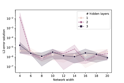
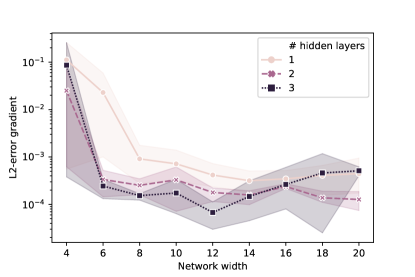
Refer to captionRefer to caption

Figure 13. Average error of PDE solution approximation and its gradient and 95% confidence interval of different combination of # of layers and net width. Left: error model. Right: Error grad model

Acknowledgements

This work was supported by the Alan Turing Institute under EPSRC grant no. EP/N510129/1.

References

  • [1] C. Bayer and B. Stemper. Deep calibration of rough stochastic volatility models. arXiv:1810.03399, 2018.
  • [2] C. Beck, S. Becker, P. Grohs, N. Jaafari, and A. Jentzen. Solving stochastic differential equations and kolmogorov equations by means of deep learning. arXiv:1806.00421, 2018.
  • [3] C. Beck, L. Gonon, and A. Jentzen. Overcoming the curse of dimensionality in the numerical approximation of high-dimensional semilinear elliptic partial differential equations, 2020.
  • [4] D. Belomestny, S. Hafner, T. Nagapetyan, and M. Urusov. Variance reduction for discretised diffusions via regression. Journal of Mathematical Analysis and Applications, 458(1):393–418, 2018.
  • [5] D. Belomestny, L. Iosipoi, and N. Zhivotovskiy. Variance reduction via empirical variance minimization: convergence and complexity. arXiv:1712.04667, 2017.
  • [6] J. Berner, P. Grohs, and A. Jentzen. Analysis of the generalization error: Empirical risk minimization over deep artificial neural networks overcomes the curse of dimensionality in the numerical approximation of black–scholes partial differential equations. SIAM Journal on Mathematics of Data Science, 2(3):631–657, Jan 2020.
  • [7] M. T. Blanka Horvath, Aitor Muguruza. Deep learning volatility: A deep neural network perspective on pricing and alibration in (rough) volatility models. arXiv:1901.09647, 2019.
  • [8] M. Broadie, Y. Du, and C. C. Moallemi. Risk estimation via regression. Operations Research, 63(5):1077–1097, 2015.
  • [9] Q. Chan-Wai-Nam, J. Mikael, and X. Warin. Machine learning for semi linear pdes. Journal of Scientific Computing, 79(3):1667–1712, 2019.
  • [10] L. Chizat and F. Bach. On the global convergence of gradient descent for over-parameterized models using optimal transport. In Advances in neural information processing systems, pages 3036–3046, 2018.
  • [11] S. N. Cohen and R. J. Elliott. Stochastic calculus and applications. Springer, 2015.
  • [12] R. Cont and Y. Lu. Weak approximation of martingale representations. Stochastic Processes and their Applications, 126(3):857–882, Mar 2016.
  • [13] J. Cvitanic, J. Zhang, et al. The steepest descent method for forward-backward sdes. Electronic Journal of Probability, 10:1468–1495, 2005.
  • [14] J. B. Diederik P. Kingma. Adam: A method for stochastic optimization. arXiv:1412.6980, 2017.
  • [15] S. S. Du, X. Zhai, B. Poczos, and A. Singh. Gradient descent provably optimizes over-parameterized neural networks. arXiv:1810.02054, 2018.
  • [16] D. Elbrächter, P. Grohs, A. Jentzen, and C. Schwab. Dnn expression rate analysis of high-dimensional pdes: Application to option pricing. Constructive Approximation, May 2021.
  • [17] P. Glasserman. Monte Carlo methods in financial engineering. Springer, 2013.
  • [18] L. Gonon, P. Grohs, A. Jentzen, D. Kofler, and D. Šiška. Uniform error estimates for artificial neural network approximations for the heat equation. IMA Journal Numerical Analysis, 2021.
  • [19] I. Goodfellow, J. Shlens, and C. Szegedy. Explaining and harnessing adversarial examples. arXiv:1412.6572, 2014.
  • [20] P. Grohs, F. Hornung, A. Jentzen, and P. von Wurstemberger. A proof that artificial neural networks overcome the curse of dimensionality in the numerical approximation of Black-Scholes partial differential equations. arXiv:1809.02362, 2018.
  • [21] P. Grohs, A. Jentzen, and D. Salimova. Deep neural network approximations for monte carlo algorithms, 2019.
  • [22] J. Han, A. Jentzen, et al. Solving high-dimensional partial differential equations using deep learning. arXiv:1707.02568, 2017.
  • [23] J. Han and J. Long. Convergence of the deep bsde method for coupled fbsdes. Probability, Uncertainty and Quantitative Risk, 5(1):1–33, 2020.
  • [24] P. Henry-Labordere. Deep primal-dual algorithm for BSDEs: Applications of machine learning to CVA and IM. Available at SSRN 3071506, 2017.
  • [25] A. Hernandez. Model calibration with neural networks. Available at SSRN 2812140, 2016.
  • [26] B. Horvath, A. Muguruza, and M. Tomas. Deep learning volatility. Available at SSRN 3322085, 2019.
  • [27] K. Hu, Z. Ren, D. Šiška, and L. Szpruch. Mean-Field Langevin Dynamics and Energy Landscape of Neural Networks. Annales de l’Institute Henry Poincaré Proability and Statistics, 57(4):2043–2065, 2021.
  • [28] C. Huré, H. Pham, and X. Warin. Some machine learning schemes for high-dimensional nonlinear PDEs. arXiv:1902.01599, 2019.
  • [29] M. Hutzenthaler, A. Jentzen, T. Kruse, and T. A. Nguyen. A proof that rectified deep neural networks overcome the curse of dimensionality in the numerical approximation of semilinear heat equations. SN Partial Differential Equations and Applications, 1(2), Apr 2020.
  • [30] A. Itkin. Deep learning calibration of option pricing models: some pitfalls and solutions. arXiv:1906.03507, 2019.
  • [31] A. J. Jacquier and M. Oumgari. Deep PPDEs for rough local stochastic volatility. Available at SSRN 3400035, 2019.
  • [32] A. Jentzen, D. Salimova, and T. Welti. A proof that deep artificial neural networks overcome the curse of dimensionality in the numerical approximation of Kolmogorov partial differential equations with constant diffusion and nonlinear drift coefficients. arXiv:1809.07321, 2018.
  • [33] N. Krylov. On Kolmogorov’s equations for finite dimensional diffusions. In Stochastic PDE’s and Kolmogorov Equations in Infinite Dimensions, pages 1–63. Springer, 1999.
  • [34] N. V. Krylov. Introduction to the theory of random processes. American Mathematical Society, 2002.
  • [35] G. Kutyniok, P. Petersen, M. Raslan, and R. Schneider. A theoretical analysis of deep neural networks and parametric pdes, 2020.
  • [36] Y. LeCun, Y. Bengio, and G. Hinton. Deep learning. Nature, 521(7553):436, 2015.
  • [37] S. Liu, A. Borovykh, L. A. Grzelak, and C. W. Oosterlee. A neural network-based framework for financial model calibration. arXiv:1904.10523, 2019.
  • [38] W. A. McGhee. An artificial neural network representation of the SABR stochastic volatility model. SSRN 3288882, 2018.
  • [39] S. Mei, A. Montanari, and P.-M. Nguyen. A mean field view of the landscape of two-layer neural networks. Proceedings of the National Academy of Sciences, 115(33):E7665–E7671, 2018.
  • [40] G. Milstein and M. Tretyakov. Solving parabolic stochastic partial differential equations via averaging over characteristics. Mathematics of computation, 78(268):2075–2106, 2009.
  • [41] N. J. Newton. Variance reduction for simulated diffusions. SIAM Journal on Applied Mathematics, 54(6):1780–1805, 1994.
  • [42] B. Øksendal. Stochastic differential equations. In Stochastic differential equations, pages 65–84. Springer, 2003.
  • [43] C. Reisinger and Y. Zhang. Rectified deep neural networks overcome the curse of dimensionality for nonsmooth value functions in zero-sum games of nonlinear stiff systems, 2020.
  • [44] G. M. Rotskoff and E. Vanden-Eijnden. Neural networks as interacting particle systems: Asymptotic convexity of the loss landscape and universal scaling of the approximation error. arXiv:1805.00915, 2018.
  • [45] M. Sabate-Vidales, D. Šiška, and L. Szpruch. Solving path dependent pdes with LSTM networks and path signatures, 2020.
  • [46] C. S. Sergey Ioffe. Batch normalization: Accelerating deep network training by reducing internal covariate shift. arXiv:1502.03167, 2015.
  • [47] J. Sirignano and K. Spiliopoulos. DGM: A deep learning algorithm for solving partial differential equations. arXiv:1708.07469, 2017.
  • [48] J. Sirignano and K. Spiliopoulos. Mean field analysis of neural networks: A central limit theorem. Stochastic Processes and their Applications, 2019.
  • [49] H. Stone. Calibrating rough volatility models: a convolutional neural network approach. arXiv:1812.05315, 2018.
  • [50] Z. Wang and S. Tang. Gradient convergence of deep learning-based numerical methods for bsdes. Chinese Annals of Mathematics, Series B, 42(2):199–216, 2021.
  • [51] E. Weinan, J. Han, and A. Jentzen. Deep learning-based numerical methods for high-dimensional parabolic partial differential equations and backward stochastic differential equations. Communications in Mathematics and Statistics, 5(4):349–380, 2017.