Efficient estimation of autocorrelation spectra
Abstract
The performance of Markov chain Monte Carlo calculations is determined by both ensemble variance of the Monte Carlo estimator and autocorrelation of the Markov process. In order to study autocorrelation, binning analysis is commonly used, where the autocorrelation is estimated from results grouped into bins of logarithmically increasing sizes.
In this paper, we show that binning analysis comes with a bias that can be eliminated by combining bin sizes. We then show binning analysis can be performed on-the-fly with linear overhead in time and logarithmic overhead in memory with respect to the sample size. We then show that binning analysis contains information not only about the integrated effect of autocorrelation, but can be used to estimate the spectrum of autocorrelation lengths, yielding the height of phase space barriers in the system. Finally, we revisit the Ising model and apply the proposed method to recover its autocorrelation spectra.
I Introduction
The theoretical treatment of problems at the forefront of physics research often involves integration of a highly non-trivial function over a many-dimensional space. Prominent examples include condensed matter with strong electronic correlation (loewdin-acp07, ), interacting nuclear matter, lattice quantum field theories, as well as systems with geometrical frustration. For these problems, brute force attempts at a solution are usually met with an “exponential wall”, i.e., a cost in resources that rises exponentially with the complexity of the system under study.
Markov chain Monte Carlo (MCMC) techniques evaluate the integral stochastically by performing a random walk in the high-dimensional space (LandauBinder05, ; krauth-statmech06, ). They are ideally suited for high-dimensional integrals, and have led to many breakthroughs in the aforementioned fields. Nevertheless, major generic challenges such as infinite variances (shi-pre16, ) and the fermionic sign problem (loh-prb-1990, ) remain, and this has led the community to create more and more elaborate Markov chain Monte Carlo algorithms (gubernatis-latticemc16, ). In order to do so, it is important to be able to analyze the statistical properties of the algorithms we create. Otherwise, we can only rely on our physical intuition and cumbersome trial-and-error to improve our method.
Due to the remarkable simplicity of the central limit theorem, the performance of a plain Monte Carlo integration is only affected by the variance of the integrand, which we can trivially estimate. We can use this in an attempt to construct “improved estimators” or to rebalance the deterministic and stochastic part of the algorithm (liu-mc01, ).
However, as soon as we sample along a Markov chain, the performance is now a combination of the variance of the integrand and the total effect of autocorrelation along the Markov chain (sokal-bosonic92, ). In order to analyze and improve our algorithm, we must disentangle the properties of the Markov chain, which relates to the efficiency of the moves we chose, from the properties of the space under study.
Two techniques are in wide use to estimate autocorrelation: (i) direct measurement of the autocorrelation function (madras-sokal-jsp88, ; janke-stat02, ) and (ii) binning or blocking analysis(flyvbjerg-jcp91, ). Measurement of the autocorrelation function is straightforward, and allows one to analyze the structure of the Markov chain in more detail. However, it is also expensive in terms of time and memory, and in order for estimators to have finite variance, it usually requires an ad hoc regularization of the sum, potentially introducing bias. Binning analysis, on the other hand, can be performed considerably faster and with less memory. However, it only provides an estimate for the integrated effect of autocorrelation.
In this paper, we first show that the logarithmic binning analysis (Sec. III.1), while asymptotically correct, has a practical bias. We show a simple trick to correct for that bias (Sec. III.2). We then show how to perform the binning analysis with only a constant overhead in time per move (Sec. III.4). We then show that the logarithmic binning analysis can not only be used to gauge the total effect of autocorrelation, but can also be used to estimate the height and strength of phase space barriers present in the system (Sec. IV) and illustrate the method on the Ising model (Sec. V).
II Review: Markov chain spectra
In order to move forward with the algorithm, it is useful to review a couple of key points on Markov chains and Monte Carlo integration along Markov chains (grimmett-markov12, ). For simplicity, we will focus on finite reversible Markov chains, but the results are equally applicable to infinite and non-reversible chains. Unless explicitly noted, we only consider stationary Markov chains (see later).
A Markov chain is characterized by a number of states and an transition matrix encoding the probabilities to go from state to state . We require the Markov chain to be ergodic (irreducible), which roughly means that each state can be reached from any other state in a finite number of steps. Each ergodic Markov chain tends to a stationary distribution . We would like to choose in such a way that the stationary distribution matches the distribution we would like to sample. For this, it is sufficient to require the Markov chain to be in detailed balance (reversibility) with respect to ; formally: .
Using the Perron–Frobenius theorem, one can show that a Markov chain satisfying above criteria has the following spectral decomposition (grimmett-markov12, ):
| (1) |
where are eigenvalues and are a set of vectors forming an orthonormal basis. We see that indeed is a stationary distribution of , as is a right eigenvector of with eigenvalue 1: . However, there are additional modes in Eq. (1) that decay on a characteristic scale in Markov time, where
| (2) |
The determines the so-called spectral gap of the Markov chain, defined as . The corresponding gives a worst-case estimate for how many steps it takes a Markov chain to reach a stationary distribution. It thus provides an important lower bound for the number of initial steps that should be discarded in a simulation, and is sometimes called exponential autocorrelation time (sokal-bosonic92, ; sokal-lecture96, ).
Now let us consider random variable with expectation value . We would like to estimate using a suitable Markov chain. To do so, we construct the Markov chain Monte Carlo estimator by sampling steps along the Markov chain, i.e.,
| (3) |
If we have sufficiently thermalized the run, we sample according to the stationary distribution , and the estimator provides an unbiased estimate for the expectation value of , i.e., . For the variance, however, one finds (sokal-lecture96, ):
| (4) |
where is the autocorrelation function of and distance or “lag” in Markov time, defined as:
| (5) |
where . The autocorrelation function starts at 1 for , indicating that a measurement is always perfectly correlated with itself, and drops off exponentially in both directions. The decay again depends on the characteristic decay times (2). However, the coefficient depends on the influence of the corresponding “mode” of the Markov chain on the quantity under study.
Taking the limit in Eq. (4), we find the familiar expression (sokal-bosonic92, ; liu-mc01, ; berg-mcmc04, ):
| (6) |
where we have defined the integrated autocorrelation time for , given by:111Another common convention is to define as the sum of of the autocorrelation function. In this case, the right-hand side of Eq. (7) is 2+1.
| (7) |
The integrated autocorrelation time is the total effect of autocorrelation on the variances. Comparing Eq. (6) with the central limit theorem for non-autocorrelated samples, we can say autocorrelation reduces the number of independent samples from to .
Eq. (6) makes it clear why the estimating the autocorrelation time is important when designing a new Monte Carlo algorithm: the variance of the estimate is a combination of the intrinsic efficiency of the Monte Carlo procedure, which only depends on the quantity and the space under study, and the efficiency of the Markov chain in exploring said space. These two things need to be disentangled in order to gauge whether we need to improve the quality of our proposed moves or work on improving the estimator itself.
III Logarithmic Binning Analysis
III.1 Review: Autocorrelation estimates
One strategy to estimate the integrated autocorrelation time is to turn Eqs. (5) and (7) into an estimator. One usually first constructs an estimator for the autocovariance function (sokal-lecture96, ):
| (8) |
By normalizing the autocovariance function we obtain an estimator for the autocorrelation function:
| (9) |
which we can sum up to obtain an estimator for the integrated autocorrelation time:
| (10) |
where we have introduced a window function that should in principle be taken as .
In practice, there are two problems with this approach: first, the noise-to-signal ratio in the autocorrelation estimator blows up as
| (11) |
as the autocorrelation function drops exponentially with some time scale , while only data points are available in Eq. (8). Plugging this into Eq. (10), the variance of the sum diverges. To remedy that one has to choose a hard cutoff in the window function , truncating the sum for , introducing bias (madras-sokal-jsp88, ; janke-stat02, ). Secondly, the procedure is computationally expensive, requiring of time and of memory in the case of a cutoff chosen a priori, or time and of memory if the cutoff is determined a posteriori.
The other strategy is to construct a binning estimator : instead of sampling over individual measurements, we group them into non-overlapping bins . Each bin is the mean of consecutive measurements, so the zeroth bin contains the mean of the inital samples, ; the first bin contains the mean of the next samples; and so on:
| (12) |
Comparing Eqs. (12) and Eq. (3), we find that each bin can be understood as a small sampling procedure with the sample size replaced by the bin size . Thus, for large enough , the variance of the individual bin means is given by Eq. (6), which we can estimate from the data since we have bins:
| (13) |
(We emphasize the difference in notation: is the variance of the mean estimator, or in other words the squared standard error of the mean, while is an estimator of the variance.)
Thus, we can turn Eq. (6) into a binned estimator for the integrated autocorrelation time (berg-mcmc04, ):
| (14) |
In the limit , Eq. (6) trivially ensures that the bias, defined as:
| (15) |
vanishes. For a finite and fixed number of simulation steps , however, one has to make a trade-off between bias, which improves with , and the statistical error of the integrated autocorrelation time estimator (14), which increases as .

Because a single, ad hoc choice for makes it difficult to gauge this tradeoff, one usually performs what is known as blocking or (logarithmic) binning analysis (flyvbjerg-jcp91, ). There, one computes for a set of logarithmically spaced . This can be done efficiently by combining two lower-level bins into higher-level bins according to:
| (16) |
which, for a precomputed set of measurements, can be performed in time and of additional memory (see Fig. 1a).
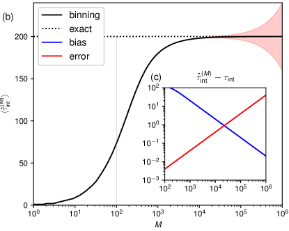
One then plots the autocorrelation estimate (14) over and assesses the trade-off, usually by visual inspection. As an example, let us take an autocorrelation function with a single time scale . The mean of the autocorrelation estimator (7) for different values of is shown as solid black line in Fig. 1b: we see that for , approaches the true value of , represented as dotted black line. (Note that since both the effect of autocorrelation with negative and positives offsets are included in our definition.) At the same time, the statistical error starts to grow, signified by the red interval (gubernatis-latticemc16, ).
III.2 Bias correction
Fig. 1c makes the trade-off between systematic bias (blue), computed from Eq. (15), and statistical error (red), estimated from the asymptotic expression, in the logarithmic binning analysis explicit. We see that the autocorrelation estimate converges relatively slowly, , to the true result. Since the statistical error rises relatively quickly, , as well, it can be difficult to find a good tradeoff between the two errors.
To understand the bias, let us consider the expectation value for the binned variance estimator (13):
| (17) |
Using Eq. (3) and employing the stationarity condition (we have “thermalized” the run), one can write Eq. (17) in terms of the autocorrelation function (5) as follows:
| (18) |
where is the scaled triangular window function of width :
| (19) |
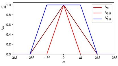
The values of the window for and are plotted in Fig. 2a (red curves). The convolution of the autocorrelation function with the window expresses the fact that we discard correlations that cross bin boundaries. (Those correlations could be encoded by constructing a covariance matrix across bins or bin sizes.)
Examining Eq. (19), we see that the autocorrelation time estimator Eq. (14) must have a significant bias, as we already cut away some of the short-length autocorrelation, e. g., the correlation of the last measurement of the ’th bin with the first measurement of the ’st bin.
However, we can use the fact that we have logarithmically spaced bins to our advantage and construct a trapezoid window function by linear combination:
| (20) |
Such a new window function is plotted as blue curve in Fig. 2a: we see that we take autocorrelations up to length fully into account, and include diminishing contributions from lengths to . The corresponding bias-corrected autocorrelation estimator is given by:
| (21) |
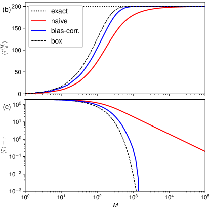
Fig. 2b compares the naive estimator (red curve) using Eq. (14) with the bias-corrected estimator (blue curve) using Eq. (21), again for a single autocorrelation mode with . For comparison, the explicit summation (7) of the autocorrelation function with a hard cutoff is shown as black dashed curve. We see that the bias-corrected estimator approaches the exact value of nearly as fast as the explicit summation.
Examining the bias (Fig. 2c), we find that while the bias of the naive estimator drops as , the bias of the corrected estimator drops as , as we include all short-range autocorrelation contributions explicitly. This results in a stable and pronounced “plateau” in the improved estimator, the height of which yields the integrated autocorrelation time.
The statistical error of both naive and improved estimator scale as , but the reduction of bias comes at the cost of an at most two-fold increase in the statistical error. This is a beneficial tradeoff: suppose we want to choose such that bias and stastical error have the same asymptotic behaviour with . For the naive estimator, we should choose , which yields a total error of (frezzotti-qcd, ). For the improved estimator, we can choose , where is a parameter, which improves the total error to . In the case where is unknown, the choice with still yields better asymptotic behavior than in the naive case.
III.3 Example: vector autoregression
To illustrate and test the effect of bias correction, we use a first-order vector autoregression model (VAR(1) model). One of the simplest autocorrelated Markov processes, the VAR(1) model can be written as (enders-ts04, ):
| (22) |
where is a random -vector for the -th step of the process, is a constant vector, is an matrix, and is a set of random vectors identically and independently distributed according to , introducing white noise into the system 222We note that the VAR(1) model has an infinite state space and thus the Markov chain review of Sec. II is not directly applicable. However, the setup is easily generalized to infinite state spaces for which all the conclusions in this paper remain valid..
For , the process will tend to a stationary case. The autocorrelation function is then simply given by (enders-ts04, ):
| (23) |
and the covariance matrix of is the solution to the following Lyapunov (matrix) equation:
| (24) |
VAR(1) models are most commonly used as a fitting method for autocorrelated observations (cf. Sec. IV.1). We are going to run it in the opposite direction and use Eq. (22) as prescription for generating an autocorrelated dataset. We used two components () and generated the propagation matrix from two eigenvalues and rotated the eigenbasis by degrees to introduce coupling between the components. We then generated runs of configurations each, and measured the first component for each configuration.
The integrated autocorrelation is then given analytically from Eq. (23):
| (25) |
where denotes the -component of the respective matrix. (The covariance appears in Eq. (25) because when we truncate to form the observable , we silently discard the cross-correlations in the normalization of the autocovariance function.)
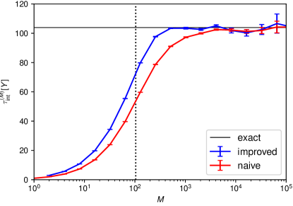
Fig. 3 compares results from the naive estimator (14) with ones from the bias-corrected estimator (21) for the autocorrelation time of the VAR(1) model outlined above. The exact value for from Eq. (25) is shown as black solid line as well as black dashed line. As expected from Sec. III.2, the naive estimator (red curve) significant bias that persists for several orders of magnitude of even after exceeds the integrated autocorrelation time. For large , where the bias decays, its effect intermingles with the statistcal uncertainty, which renders the extraction of the autocorrelation time unreliable.
The improved estimator (blue curve), on the other hand, converges exponentially to a stable plateau as soon as exceeds . By extracting the height of the plateau one obtains a reliable estimate for .
As discussed in Sec. III.2, we see that the improved estimator has statistical error bars that are about twice as large as the naive estimator, but the exponential drop of the bias allows us to choose a lower , which yields a better estimate of the plateau height and thus .
III.4 Online estimation in linear time
Given a Monte Carlo run with measurements, we can perform the logarithmic binning analysis in time: computing the variance over bins and combining bins both take time, and the number of bins shrinks by a factor of each time we double the bin size. We find:
| (26) |
For storing the variances for the different , we need of memory. However, we also need to store the measurements in order to perform the binning analysis on them. This takes an additional of memory, which grows prohibitively quickly for large runs.
We would like to eliminate this memory requirement, and are thus looking for an algorithm that can perform the analysis online, i.e., processing measurements one at a time without the need to store the whole data series.
One can solve this problem by first realizing that the variance can be estimated online (knuth-aocp2, ; chan-stat83, ): in the simplest case, we initialize three accumulators . Each data point is first added to the bin accumulator . Once we collected measurements, we update the accumulator according to and reset the bin . At the end, we combine the results to the variance 333We note here that the separate accumulation of and may cause stability problems; more advanced accumulation techniques can be used instead at little additional overhead.(chan-stat83, ). We can therefore do a binning analysis by setting up a triplet of accumulators for each , and add every data point to each of the accumulators. One therefore reduces the memory overhead to and the runtime to (ambegaokar-ajp10, ).
This solves the memory issue, but can still amount to a significant runtime overhead. We can however still improve the runtime to by realizing that we can reuse the bin results from the bin size for the bin size : instead of adding each data point to every accumulator, we only add it to the lowest level (). Then whenever, we “empty” a bin accumulator at the level , we not only update the partial sums , but also add the result to the bin accumulator at the next level: 444During peer review, the author was made aware of unpublished work by H. G. Evertz, who implemented a similar strategy in 1990..
By the same argument as in Eq. (26), the logarithmic binning analysis can thus be performed in time while keeping the memory scaling. This is a negligible overhead in most Monte Carlo calculations: even in the case of VAR(1) model simulations (Sec. IV.3), where the Monte Carlo updates are next to trivial, the accumulation amounts to less than 10% computing time.
IV Logarithmic Spectral Analysis
IV.1 Review: Spectrum estimates
As we have seen in the previous section, binning analysis allows us to estimate the total effect of autocorrelation. However, ideally, we would also like to estimate the most important individual contributing time scales in Eq. (5). In other words, we would like to find an approximation:
| (27) |
where the index runs over the dominant time scales. (The tacit assumption will be justified in Sec. IV.4.)
Aside from analytical arguments, which are restricted to simple Markov chains, one can use Eq. (8) to get an estimate for the autocorrelation function from and then attempt to fit a set of exponential decays to it. An elegant way of fitting is to employ the linear prediction method (prony, ; rahmn-ieee87, ): one first attempts to find an auxiliary model (cf. Sec. III.3) which best reproduces the observed , and then extracts the using Eq. (23). Once an approximation (27) is obtained, one can use Eq. (7) to estimate the integrated autocorrelation time.
Since the method relies on the estimator (8), the drawbacks outlined in Sec. III.1 carry over to the spectrum estimation: firstly, the unfavorable computational scaling of space and time is also present here. Secondly, linear prediction is susceptible to noise levels exceeding , which means one again has to introduce a cutoff because of the noise-to-signal problem (cf. Ref. deylon-pre17, ).
IV.2 Spectral analysis from logarithmic binning
Because of the computational expense of the conventional spectrum estimators, we ideally would like estimate the spectrum from the logarithmic binning analysis, which can be performed quickly, in time, and with little additional memory, .
In order to do so, we first examine the influence of a single mode with decay on the binning analysis. For a single , Eq. (18) gives:
| (28) |
The first term on the r.h.s. of Eq. (28) is the asymptotic value, the integrated autocorrelation time, and we see that the difference indeed drops as , as observed in Sec. III.2.
In order to analyze the spectrum, we remove the trivial term, and define:
| (29) |
Similarly, we combine the binning results as follows:
| (30) |
Using Eqs. (5) and (18), one then finds:
| (31) |
with the coefficient .
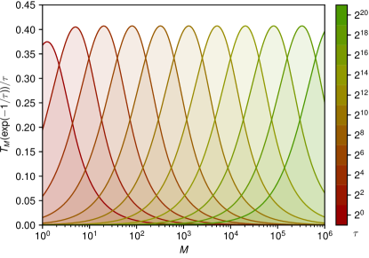
The function , normalized by the corresponding , is plotted in Fig. 4 over . Different curves correspond to different values of . We see that each value of can be translated into a Gaussian-like structure in centered around , which is then observed by the corresponding . One can show that the maximum is located at
| (32) |
where is the Lambert function.
Eq. (31) is thus again a fitting problem, where is the observed data vector from logarithmic binning, and and are the model coefficients. Unlike the case where we compute the spectrum from the autocorrelaiont estimator (cf. Sec. IV.1), the data points are not equidistantly spaced, and we unfortunately cannot use linear prediction or other variants of Prony’s method.
A simple but sufficiently accurate method to resolve the interdependency in Eq. (31) is to use a mesh for and only fit the coefficients. Studying Fig. 4 and Eq. (32), we strive for “equispaced” curves in . Therefore, we make logarithmic ansatz for the decay times, i.e.,
| (33) |
and compute the corresponding using Eq. (2). Eq. (31) can then be written as an ordinary least squares problem:
| (34) |
where is the vector of observations , is the fitting matrix , and is the vector of coefficients .
On real binning data, it is important to use a generalized least squares method (aitken-prsed34, ) instead of Eq. (34). This is because the statistical uncertainty in raises as as evident from Fig. 1b, so the data points cannot be treated with equal weight. We empirically found that one need not treat the full covariance matrix, and instead approximate . The problem is then reformulated as:
| (35) |
where and .
Both the ordinary (34) and the generalized least squares problem (35) are poorly conditioned. (The condition number is usually of the order .) To battle such a problem, regularization techniques are commonly used, where a small regularization term is added to the cost function (35). In our case, we found that large values of are needed to stabilize regressions for , introducing significant systematic bias.
Instead, we exploit the fact that and use the non-negative least squares method (NNLS), where we minimize Eq. (35) subject to a non-negativity constraint (lawson-hanson-ls, ). We find that NNLS method is numerically stable when run on our fitting problem. After the NNLS procedure, the fitted coefficients now give the approximation to the autocorrelation spectrum on a logarithmic mesh :
| (36) |
Once we have found an approximation (36) to the autocorrelation function, we can use it to reconstruct a filtered version of the binning analysis through Eq. (29) and, more importantly, find an estimate for the integrated autocorrelation time through Eq. (7) that does not rely on visual inspection or an external parameter.
IV.3 Example: vector autoregression for
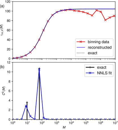
As an example, we return to our VAR(1) model of Sec. III.3. We again use two components () and generated the propagation matrix from two eigenvalues , which correspond to . We rotated the eigenbasis by degrees to introduce coupling between the components. From Eq. (25), we find that the expansion coefficients are . We then generated configurations, and measured the first component for each configuration.
The corresponding (biased) autocorrelation estimator from Eq. (14) is shown in Fig. 5a (red crosses). The exact curve in dotted black is given for comparison. The corresponding spectral analysis is given in Fig. 5b. For simplicity, we chose in Eq. (33), which generates an identical grid for binning analysis and spectral analysis. The NNLS fitted coefficients are shown as blue crosses, and we can see that they closely follow the analytic peaks in both location and magnitude.
The blue curve in Fig. 5a shows the reconstructed binning data, by plugging the model coefficients into Eq. (29): we see that the curve smoothens out the statistical uncertainties at high due to the use of weights in the least squares procedure, shows the correct monotonic behavior due to the non-negativity constraint in the least squares procedure, and overall follows the analytic curve (dotted black) closely. Similarly, computing the autocorrelation time from the spectral analysis yields compared to the true value of .
IV.4 Metropolis–Hastings Monte Carlo
By making a logarithmic ansatz (33) for the autocorrelation times and using non-negative least squares, we have tacitly assumed that the Markov chain has no negative eigenvalues that contribute to the estimator, i.e., . This is not true in general, as can easily be seen by setting to a matrix with negative eigenvalues in Eq. (22). Negative eigenvalues express “cyclic” behavior in the Markov chain, where we get alternating correlation and anti-correlation as we move forward in Markov time.
Fortunately, one can show that the Markov chain for the Metropolis–Hastings algorithm (metropolis-jcp-1953, ; hastings-biomet-1970, ) (at least in its basic form) has no negative eigenvalues (liu-statcmp96, ). This allows us to drop the absolute value in Eq. (2) and unambiguously interpret as time scale.
In simulations of Gibbs ensembles, these time scales are related to barriers in phase space of height , where is the inverse temperature and is the energy difference to the intermittent excited state. This means we can interpret as the height of phase space barriers and the corresponding as the combined influence of barriers of that strength to the estimator in question.
V Application: Ising model
In order to perform logarithmic spectral analysis on a realistic Metropolis–Hastings Monte Carlo simulation, we consider the ferromagnetic Ising model. The results for the autocorrelation spectra are well-known there, allowing us to verify the results, while at the same time providing a realistic testbed for the method.
The Hamiltonian of the Ising model is given by (LandauBinder05, ):
| (37) |
where runs over all pairs of directly neighboring Ising spins on a square lattice with periodic boundary conditions. Since the system is finite and there is no external magnetic field, by symmetry.
We perform a Metropolis–Hastings Monte Carlo simulation for Eq. (37) with so called “typewriter sweeps”: we go through the spins of the lattice in rows from top to bottom, traversing each row from left to right. For each spin we encounter, the proposed move is to flip it .
It is well known that with these kinds of updates, the Markov chain gets “stuck” in one of two minima corresponding to a majority spin-up or spin-down configuration. These minima are separated by a phase space barrier of height , which is the energy required to form a grain boundary between spin-up and spin-down. Consequentially, the results will show spurious polarization at low temperatures or large system sizes.
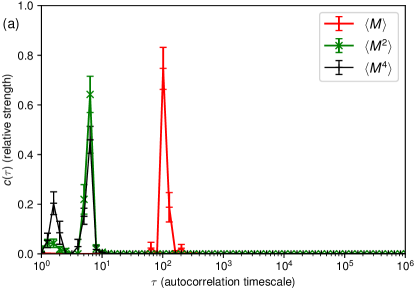
These minima and their depth can be clearly seen on the autocorrelation spectra in Fig. 6a for the mean magnetization and powers thereof, given by . We set the temperature to , just above the critical temperature. The curve for the mean magnetization shows a peak around , which corresponds to significant phase space barrier. This feature is absent in and identifying the source of the leading barrier as one that polarizes the system.
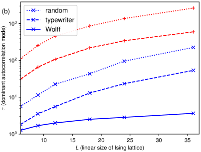
This suggests the inclusion of a global move, which just flips all spins and gets rid of the spurious polarization. To see whether such a move would solve the autocorrelation problem, we plot the location of the dominant autocorrelation mode over the linear system size for the typewriter updates (dashed curves in Fig. 6b): we see that there is a dominant autocorrelation mode in both (red dashed curve) and (blue dashed curve) that scales similarly with system size. Thus, while a move that flips all spins solves the immediate issue in , it does not solve the autocorrelation problem in larger powers and , since a global spin flip does not affect .
To make sure the problem is related to single spin flips, we compare the scaling of the dominant autocorrelation mode for the “typewriter sweeps” (dashed line), where we have a deterministic pattern of proposing spins to flip, with “random flip” sweeps (dotted line), where we choose spins at random with replacement and propose to flip each one of them. It is well-known(berg-mcmc04, ) that typewriter sweeps outperform a set of random flips because of the higher likelihood to propose clusters of spins, and this is evident in an offset of the two curves in Fig 6b. However, we see that the scaling both for (red dashed vs. dotted curve) and (blue dashed vs. dotted curve) is similar, indicating a problem common to single spin flip moves.
Eventually, the autocorrelation problem is solved by cluster updates (swensen-wang, ; Wolff89, ). Using the Wolff cluster updates (Wolff89, ), we find that the autocorrelation in is trivially solved and the dominant autocorrelation mode of (blue solid line) is considerably smaller in magnitude than when we use other updates. More importantly, we see that the scaling of the autocorrelation mode is more favorable, indicating we have overcome a phase space barrier.
Let us emphasize again that our conclusions about the effectiveness of the moves for Ising simulations are nothing “new”: the Ising model has a sufficiently simple structure and the Monte Carlo moves have a simple physical interpretation, so that we can use our physical intuition to analyze the structure of the Markov chain. The point here is to illustrate that logarithmic spectral analysis provides a way to obtain these properties without a priori knowledge or physical intuition at negligible additional computational cost. It is thus suited for more complicated models or more advanced Monte Carlo techniques.
VI Conclusions
In this paper we have shown how to perform logarithmic binning analysis and spectral analysis to extract information about the autocorrelation on Markov chain Monte Carlo runs. We have shown that these analyses can be performed at modest additional computational cost and without external parameters.
Logarithmic spectral analysis in particular allows quantitative and statistically robust analysis of the types, height, and influence of phase space barriers on the Monte Carlo result. It also can be used to get improved estimates of the integrated autocorrelation time, essential for postprocessing applications such as statistical hypothesis testing (wallerberger-pre17, ). It has the advantage of working with the existing logarithmic binning analysis data already implemented in many codes.
We feel confident that logarithmic spectral analysis will become an integral part of developing or maintaining Markov chain Monte Carlo codes: it provides a clear path on how to design and improve Markov chain moves to avoid autocorrelation effects without relying on physical intuition or trial-and-error alone, and comes at only modest additional computational cost.
The techniques outlined here are straight-forward to implement, and we encourage the reader to do so in order to get a deeper understanding. For production codes, an optimized and tested implementation of these techniques is scheduled for inclusion in the upcoming version of the ALPS core libraries (gaenko-cpc17, ).
Acknowledgements.
The author would like to thank Jia Li, Igor Krivenko and Emanuel Gull for fruitful discussions and careful review of the manuscript. MW was supported by the Simons Foundation via the Simons Collaboration on the Many-Electron Problem. This research used resources of the National Energy Research Scientific Computing Center, a DOE Office of Science User Facility supported by the Office of Science of the U.S. Department of Energy under Contract No. DE-AC02-05CH11231.References
- (1) P.-O. Löwdin, Correlation problem in many-electron quantum mechanics – I. Review of different approaches and discussion of some current ideas, in: Adv. Chem. Phys., Wiley–Blackwell, 2007, Ch. 7, pp. 207–322 (2007). doi:10.1002/9780470143483.ch7.
- (2) D. Landau, K. Binder, A Guide to Monte Carlo Simulations in Statistical Physics, Cambridge University Press, New York, NY, USA, 2005 (2005).
- (3) W. Krauth, Statistical Mechanics: Algorithms and Computations, Oxford University Press, New York, 2006 (2006).
- (4) H. Shi, S. Zhang, Infinite variance in fermion quantum Monte Carlo calculations, Phys. Rev. E 93 (2016) 033303 (Mar 2016). doi:10.1103/PhysRevE.93.033303.
- (5) E. Y. Loh, J. E. Gubernatis, R. T. Scalettar, S. R. White, D. J. Scalapino, R. L. Sugar, Sign problem in the numerical simulation of many-electron systems, Phys. Rev. B 41 (1990) 9301–9307 (1990). doi:10.1103/PhysRevB.41.9301.
- (6) J. Gubernatis, N. Kawashima, P. Werner, Quantum Monte Carlo Methods: Algorithms for Lattice Models, Cambridge University Press, 2016 (2016). doi:10.1017/CBO9780511902581.
- (7) J. S. Liu, Monte Carlo Strategies in Scientific Computing, Springer-Verlag, 2001 (2001).
- (8) A. D. Sokal, Bosonic Algorithms, in: M. Creutz (Ed.), Quantum fields Computing, World Scientific, 1992, Ch. 5, pp. 211–274 (1992). doi:10.1142/9789814439732_0005.
-
(9)
N. Madras, A. D. Sokal, The pivot
algorithm: A highly efficient monte carlo method for the self-avoiding walk,
J. Stat. Phys. 50 (1) (1988) 109–186 (Jan 1988).
doi:10.1007/BF01022990.
URL https://doi.org/10.1007/BF01022990 - (10) W. Janke, Statistical analysis of simulations: Data correlations and error estimation, in: Proceedings of the Euro Winter School Quantum Simulationsof Complex Many-Body Systems: From Theory to Algorithms, Vol. 10, John von Neumann Institute for Computing, 2002, pp. 423–445 (2002).
- (11) H. Flyvbjerg, H. G. Petersen, Error estimates on averages of correlated data, J. Chem. Phys. 91 (1989) 461 (1989). doi:10.1063/1.457480.
- (12) G. R. Grimmett, D. R. Stirzaker, Probability and random processes, 3rd Edition, Oxford University Press, 2001 (2001).
- (13) A. D. Sokal, Monte Carlo methods in statistical mechanics: Foundations and new algorithms, Lectures at the Cargèse Summer School on “Functional integration: Basics and applications”, 1996 (1996).
- (14) B. A. Berg, Introduction to Markov Chain Monte Carlo simulations and their statistical analysis 9 (2004). doi:10.1017/CBO9781107415324.004.
- (15) Another common convention is to define as the sum of of the autocorrelation function. In this case, the right-hand side of Eq. (7) is 2+1.
-
(16)
R. Frezzotti, M. Hasenbusch, U. Wolff, J. Heitger, K. Jansen,
Comparative
benchmarks of full qcd algorithms, Comput. Phys. Commun. 136 (1) (2001) 1 –
13 (2001).
doi:https://doi.org/10.1016/S0010-4655(00)00242-3.
URL http://www.sciencedirect.com/science/article/pii/S0010465500002423 - (17) W. Enders, Applied Econometric Time Series, Wiley Series in Probability and Statistics, J. Wiley, 2004 (2004).
- (18) We note that the VAR(1) model has an infinite state space and thus the Markov chain review of Sec. II is not directly applicable. However, the setup is easily generalized to infinite state spaces for which all the conclusions in this paper remain valid.
- (19) D. E. Knuth, The Art of Computer Programming; Volume 2: Seminumerical Algorithms, 3rd Edition, Addison-Wesley, Boston, MA, USA, 1997 (1997).
- (20) T. F. Chan, G. H. Golub, R. J. LeVeque, Algorithms for computing the sample variance: Analysis and recommendations, The American Statistician 37 (3) (1983) 242–247 (1983). doi:10.2307/2683386.
- (21) We note here that the separate accumulation of and may cause stability problems; more advanced accumulation techniques can be used instead at little additional overhead.(chan-stat83, ).
- (22) V. Ambegaokar, M. Troyer, Estimating errors reliably in Monte Carlo simulations of the Ehrenfest model, Am. J. Phys. 78 (2) (2010) 150–157 (2010). doi:10.1119/1.3247985.
- (23) During peer review, the author was made aware of unpublished work by H. G. Evertz, who implemented a similar strategy in 1990.
- (24) R. de Prony, Essai experimentale et analytique, J. Ecole Polytechnique (1795) 24–76 (1795).
- (25) M. Rahman, K.-B. Yu, Total least squares approach for frequency estimation using linear prediction, IEEE Trans. Acoust. 35 (1987) 1440 – 1454 (11 1987). doi:10.1109/TASSP.1987.1165059.
-
(26)
F. Delyon, B. Bernu, M. Holzmann,
Confidence and
efficiency scaling in variational quantum monte carlo calculations, Phys.
Rev. E 95 (2017) 023307 (Feb 2017).
doi:10.1103/PhysRevE.95.023307.
URL https://link.aps.org/doi/10.1103/PhysRevE.95.023307 - (27) A. C. Aitken, On least-squares and linear combinations of observations, Proc. R. Soc. Edinburgh 55 (1934) 42–48 (1934).
- (28) C. L. Lawson, R. J. Hanson, Solving Least Squares Problems, Prentice-Hall, 1974 (1974).
- (29) N. Metropolis, A. W. Rosenbluth, M. N. Rosenbluth, A. H. Teller, E. Teller, Equation of state calculations by fast computing machines, J. Chem. Phys. 21 (6) (1953) 1087–1092 (1953). doi:http://dx.doi.org/10.1063/1.1699114.
- (30) W. K. Hastings, Monte Carlo sampling methods using Markov chains and their applications, Biometrika 57 (1) (1970) 97–109 (1970). doi:10.1093/biomet/57.1.97.
- (31) J. S. Liu, Metropolized independent sampling with comparisons to rejection sampling and importance sampling, Stat. Comput. 6 (2) (1996) 113–119 (1996). doi:10.1007/BF00162521.
- (32) R. H. Swendsen, J.-S. Wang, Nonuniversal critical dynamics in monte carlo simulations, Phys. Rev. Lett. 58 (1987) 86–88 (Jan 1987). doi:10.1103/PhysRevLett.58.86.
- (33) U. Wolff, Collective monte carlo updating for spin systems, Phys. Rev. Lett. 62 (1989) 361–364 (Jan 1989). doi:10.1103/PhysRevLett.62.361.
- (34) M. Wallerberger, E. Gull, Hypothesis testing of scientific Monte Carlo calculations, Phys. Rev. E 96 (5) (2017) 1–6 (2017). doi:10.1103/PhysRevE.96.053303.
- (35) A. Gaenko, A. E. Antipov, G. Carcassi, T. Chen, X. Chen, Q. Dong, L. Gamper, J. Gukelberger, R. Igarashi, S. Iskakov, M. Konz, J. P. F. LeBlanc, R. Levy, P. N. Ma, J. E. Paki, H. Shinaoka, S. Todo, M. Troyer, E. Gull, Updated core libraries of the ALPS project, Comput. Phys. Commun. 213 (2017) 235–251 (2017). doi:10.1016/j.cpc.2016.12.009.