Computational Technologies for Brain Morphometry

Zicong Zhou University of Texas at Arlington, Mathematics Department, Arlington, Texas 76019-0408, zicong.zhou@mavs.uta.edu    Ben Hildebrandt University of Texas at Arlington, Mathematics Department, Arlington, Texas 76019-0408, ben.hildebrandt@mavs.uta.edu    Xi Chen University of Texas at Arlington, Mathematics Department, Arlington, Texas 76019-0408, xi.chen@mavs.uta.edu    Guojun Liao University of Texas at Arlington, Mathematics Department, Arlington, Texas 76019-0408, liao@uta.edu
(October 10, 2018)
Abstract

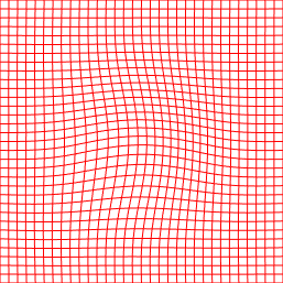
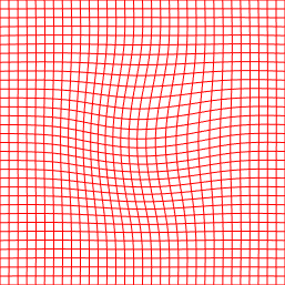
In this paper, we described a set of computational technologies for image analysis with applications in Brain Morphometry. The proposed technologies are based on a new Variational Principle which constructs a transformation with prescribed Jacobian determinant (which models local size changes) and prescribed curl-vector (which models local rotations). The goal of this research is to convince the image research community that Jacobian determinant as well as curl-vector should be used in all steps of image analysis. Specifically, we develop an optimal control method for non-rigid registration; a new concept and construction of average transformation; and a general robust method for construction of unbiased template from a set of images. Computational examples are presented to show the effects of curl-vector and the effectiveness of optimal control methods for non-rigid registration and our method for construction of unbiased template.

Keywords: Brain Morphometry, non-rigid registration, tensor based morphometry, Jacobian determinant, curl-vector, diffeomorphism

1 Introduction

In this paper, we address a key mathematical issue in brain morphometry which investigates variabilities in the shape and size of brain structures from image data. The issue is how to characterize diffeomorphisms. The prevailing paradigm in this field is to focus on Jacobian determinant J(𝑻)𝐽𝑻J(\boldsymbol{T}) of the transformation 𝑻𝑻\boldsymbol{T}, which models local size changes. We show that J(𝑻)𝐽𝑻J(\boldsymbol{T}) alone cannot completely determine a transformation. Instead, we must use both J(𝑻)𝐽𝑻J(\boldsymbol{T}) and the curl-vector of 𝑻𝑻\boldsymbol{T}, curl(𝑻)curl𝑻\text{curl}(\boldsymbol{T}), which models local rotaions, in all steps of brain morphometry studies. Specifically, we propose a new set of computational tools for morphometry studies.

  1. (1)

    For the non-rigid registration step, we develop an optimal control method which minimizes a dis-similarity measure (DS𝐷𝑆DS) under the constraints of partial differential equations such as div(𝑻)=fdiv𝑻𝑓\text{div}(\boldsymbol{T})=f, curl(𝑻)=gcurl𝑻𝑔\text{curl}(\boldsymbol{T})=g with respect to control functions f𝑓f and g𝑔g.

  2. (2)

    For the construction of an unbiased template, we propose an innovative concept of averaging a set of diffeomorphisms based on averaging the Jacobian determinants and curl-vectors of the diffeomorphisms.

  3. (3)

    For group differences, we propose to use Jacobian determinants and curl-vectors as features in TBM (tensor based morphometry) studies.

In this paper, we will focus on (1) and (2). We will demonstrate the effectiveness of our optimal control registration method mentioned in (1) and use it to perform the needed registration for constructing an unbiased template from a set of images in (2). In a future work, we will implement (3) in TBM (tensor based morphometry) studies of real data sets.

2 Effect of curl-Vectors, Variational Principle, Average of Transformations

The computational technologies described in this paper are based on a newly formulated Variational Principle [11]. We begin with an example to show the effects of the curl-vector.

2.1 Effect of curl-Vectors

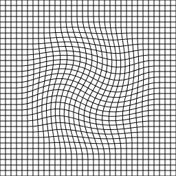
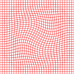
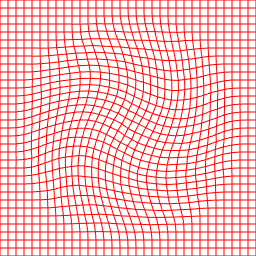
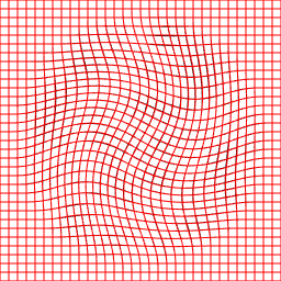
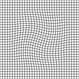
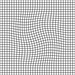
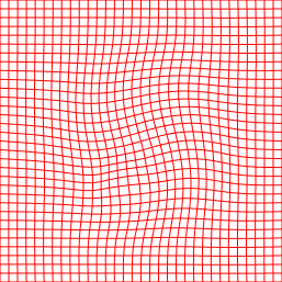
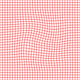
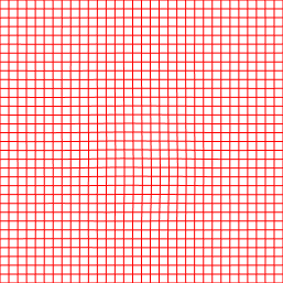
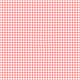
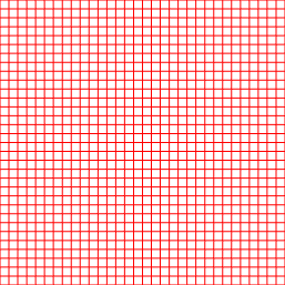
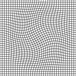
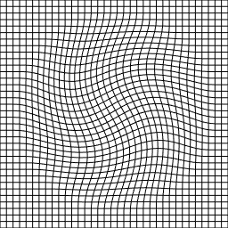
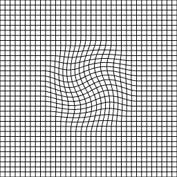
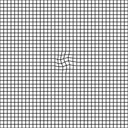
Started with a ground truth image (GT), based on portrait of Mona Lisa with 128*128 pixels shown in Figure 1(a). Then we generate two deformations 𝑫𝟏subscript𝑫1\boldsymbol{D}_{\boldsymbol{1}} and 𝑫𝟐subscript𝑫2\boldsymbol{D}_{\boldsymbol{2}} from the 128*128 uniform grid Figure 1(d) with spacing 1 (shown in 32*32) by opposite rotations such as that their Jacobian determinants are very close to 1 (in fact, between 0.996 and 1.003), and the average of their curl is 0 (the two rotations are cancelled). Figure 1(b) and 1(c) are the re-sampled images of Figure 1(a) on these two deformations Figure 1(e) and 1(f), respectively.

Resampling I0subscript𝐼0I_{0} by 𝑫1subscript𝑫1\boldsymbol{D}_{1} and 𝑫2subscript𝑫2\boldsymbol{D}_{2}, which J(𝑫2)1J(𝑫1)approximately-equals-or-equals𝐽subscript𝑫21approximately-equals-or-equals𝐽subscript𝑫1J(\boldsymbol{D}_{2})\approxeq 1\approxeq J(\boldsymbol{D}_{1}) but curl(𝑫1)curl(𝑫2)curlsubscript𝑫1curlsubscript𝑫2\text{curl}(\boldsymbol{D}_{1})\neq\text{curl}(\boldsymbol{D}_{2})

Figure 1:
Refer to caption
(a) I0subscript𝐼0I_{0} — Ground Truth
Refer to caption
(b) I1subscript𝐼1I_{1}
Refer to caption
(c) I2subscript𝐼2I_{2}
Refer to caption
(d) 𝑰𝒅𝑰𝒅\boldsymbol{Id} — uniform grid
Refer to caption
(e) 𝑫1subscript𝑫1\boldsymbol{D}_{1}
Refer to caption
(f) 𝑫2subscript𝑫2\boldsymbol{D}_{2}

2.2 Variational Principle

In this section, we describe the principles in 2D [11], where curl(𝑻)curl𝑻\text{curl}(\boldsymbol{T}) is a scalar function. A diffeomorphism 𝑻1subscript𝑻1\boldsymbol{T}_{1} on a square domain 𝔻𝔻\mathbb{D} can be deformed to 𝑻2subscript𝑻2\boldsymbol{T}_{2} with prescribed Jacobian determinant J(𝑻2(𝒙))=f0(𝒙)𝐽subscript𝑻2𝒙subscript𝑓0𝒙J(\boldsymbol{T}_{2}(\boldsymbol{x}))=f_{0}(\boldsymbol{x}) and curl(𝑻2(𝒙))=g0(𝒙)curlsubscript𝑻2𝒙subscript𝑔0𝒙\text{curl}(\boldsymbol{T}_{2}(\boldsymbol{x}))=g_{0}(\boldsymbol{x}) in the interior of 𝔻𝔻\mathbb{D}, and 𝑻(𝒙)=𝒙𝑻𝒙𝒙\boldsymbol{T}(\boldsymbol{x})=\boldsymbol{x} on the boundary of 𝔻𝔻\mathbb{D} (f0subscript𝑓0f_{0} is properly normalized for solvability). 𝑻2subscript𝑻2\boldsymbol{T}_{2} is constructed by computational minimization of the functional:

𝔻[(J(𝑻(𝒙))f0(𝒙))2+(curl(𝑻(𝒙)g0(𝒙))2]d𝒙\iint_{\mathbb{D}}{[(J(\boldsymbol{T}(\boldsymbol{x}))-f_{0}(\boldsymbol{x}))^{2}+(\text{curl}(\boldsymbol{T}(\boldsymbol{x})-g_{0}(\boldsymbol{x}))^{2}]}d\boldsymbol{x} (2.1)

subject to the constraints Δ𝑻=𝑭Δ𝑻𝑭\mathrm{\Delta}\boldsymbol{T}=\boldsymbol{F}. The variational problem is computed by a gradient decent method with respect to the control function 𝑭=(F1,F2)𝑭subscript𝐹1subscript𝐹2\boldsymbol{F}=(F_{1},F_{2}). We demonstrate the principle in next two examples below.

Example 2: Numerical Performances of Variational Principal

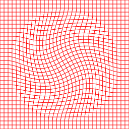
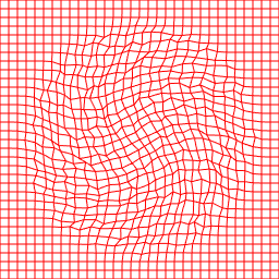
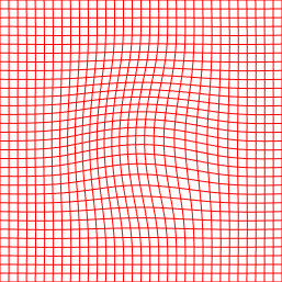
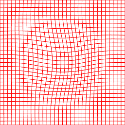
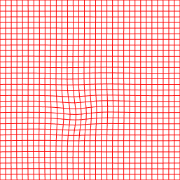
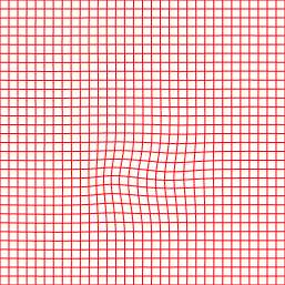
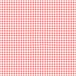
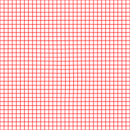
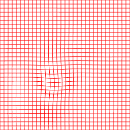
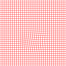
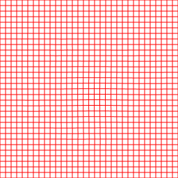
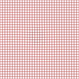
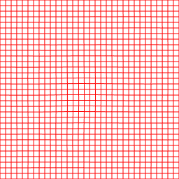
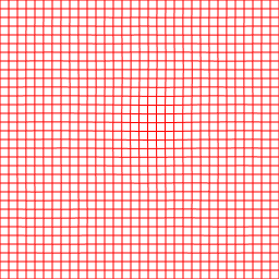
Deform 𝑫1subscript𝑫1\boldsymbol{D}_{1} to 𝑫2subscript𝑫2\boldsymbol{D}_{2} by the Variational Principle. Taking f0=J(𝑫2)subscript𝑓0𝐽subscript𝑫2f_{0}=J(\boldsymbol{D}_{2}) and g0=curl(𝑫2)subscript𝑔0curlsubscript𝑫2g_{0}=\text{curl}(\boldsymbol{D}_{2}) in the Variational Principle, in 25 iteration steps, 𝑫1subscript𝑫1\boldsymbol{D}_{1} is deformed to a transformation — 𝑫^12subscript^𝑫12\hat{\boldsymbol{D}}_{12}, as shown in Figure 2(f) that is almost identical to 𝑫2subscript𝑫2\boldsymbol{D}_{2} by prescribing its Jacobian as J(𝑫2)𝐽subscript𝑫2J(\boldsymbol{D}_{2}) and its curl as curl(𝑫2)curlsubscript𝑫2\text{curl}(\boldsymbol{D}_{2}). Total elapsed time for 25 iteration steps is 0.955899 seconds using a laptop.
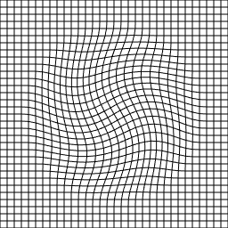
Figure 2: 𝑫1subscript𝑫1\boldsymbol{D}_{1} to 𝑫2subscript𝑫2\boldsymbol{D}_{2}
Refer to caption
(a) 𝑫1subscript𝑫1\boldsymbol{D}_{1}
Refer to caption
Refer to caption
(b) 𝑫2subscript𝑫2\boldsymbol{D}_{2}
Refer to caption
(c) step 0
Refer to caption
(d) step 2
Refer to caption
(e) step 10
Refer to caption
(f) 𝑫^12subscript^𝑫12\hat{\boldsymbol{D}}_{12} superimposed on 𝑫2subscript𝑫2\boldsymbol{D}_{2}(black)

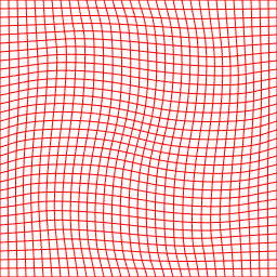
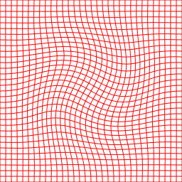
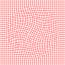
We next add noise to 𝑫1subscript𝑫1\boldsymbol{D}_{1} and deform the distorted 𝑫1subscript𝑫1\boldsymbol{D}_{1}, denoted as 𝑫𝒏1𝑫subscript𝒏1\boldsymbol{Dn}_{1}, to 𝑫2subscript𝑫2\boldsymbol{D}_{2} as before. The calculated transformation 𝑫𝒏^12subscript^𝑫𝒏12\hat{\boldsymbol{Dn}}_{12} (in red lines) by The Variational Principle is superimposed on 𝑫2subscript𝑫2\boldsymbol{D}_{2} as it shows in Figure 3(f). The red lines are almost identical to the black lines. This indicates that the results of the Variational Principle are very accurate.
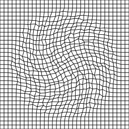
Figure 3: 𝑫𝒏1𝑫subscript𝒏1\boldsymbol{Dn}_{1} to 𝑫2subscript𝑫2\boldsymbol{D}_{2}
Refer to caption
(a) 𝑫𝒏1𝑫subscript𝒏1\boldsymbol{Dn}_{1}
Refer to caption
Refer to caption
(b) 𝑫2subscript𝑫2\boldsymbol{D}_{2}
Refer to caption
(c) step 0
Refer to caption
(d) step 550
Refer to caption
(e) step 7200
Refer to caption
(f) 𝑫𝒏^12subscript^𝑫𝒏12\hat{\boldsymbol{Dn}}_{12} superimposes on 𝑫2subscript𝑫2\boldsymbol{D}_{2}(black)

2.3 Average of Transformations

Based on the Variational Principle, we propose to average a set of transformations by averaging their Jacobian determinants and curl vectors. Given a set of transformations 𝑻isubscript𝑻𝑖\boldsymbol{T}_{i} where i=1,2,,N𝑖12𝑁i=1,2,\dots,N, we construct their average in the following steps:

  1. (1)

    Let f0=1NiNJ(𝑻i)subscript𝑓01𝑁superscriptsubscript𝑖𝑁𝐽subscript𝑻𝑖f_{0}=\frac{1}{N}\sum_{i}^{N}{J(\boldsymbol{T}_{i})} and g0=1Ni=1Ncurl(𝑻i=1)subscript𝑔01𝑁superscriptsubscript𝑖1𝑁curlsubscript𝑻𝑖1g_{0}=\frac{1}{N}\ \sum_{i=1}^{N}{\text{curl}(\boldsymbol{T}_{i=1})} as in [12]. (weighted averages can also be used)

  2. (2)

    Use f0subscript𝑓0f_{0} and g0subscript𝑔0g_{0} in the Variational Principle to calculate a transformation 𝑻𝑻\boldsymbol{T} such that J(𝑻)=f0𝐽𝑻subscript𝑓0J(\boldsymbol{T})=f_{0} and curl(𝑻)=g0curl𝑻subscript𝑔0\text{curl}(\boldsymbol{T})=g_{0}.

  3. (3)

    We define this 𝑻𝑻\boldsymbol{T} as the average of 𝑻isubscript𝑻𝑖\boldsymbol{T}_{i}, where i=1,,N𝑖1𝑁i=1,\dots,N.

Our definition of average deformation has clear geometrical meaning: The local size change ratios modeled by J(𝑻i)𝐽subscript𝑻𝑖J(\boldsymbol{T}_{i}) and the local rotations modeled by curl(𝑻i)curlsubscript𝑻𝑖\text{curl}(\boldsymbol{T}_{i}) are averaged to determine the average deformation. These two geometrical features also are biologically meaningful: the Jacobian determinant models the tissue size changes; the curl vector models the local shape change. Moreover, we directly work with transformations and thus the method applies to different registration methods.

3 Construction of Unbiased Template

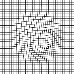
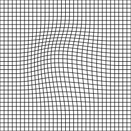
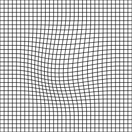
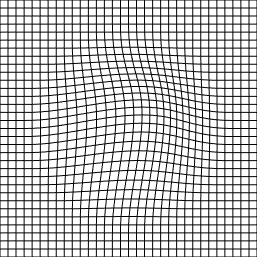
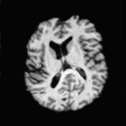
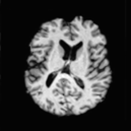
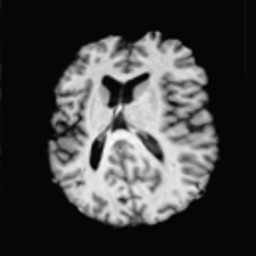
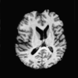
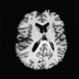
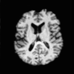
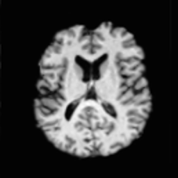
We propose a new method for construction of unbiased template from the members of an image set. The general method is described in Example 3 and a competitive computation friendly approach in Example 4. First, we obtain six brain images by re-sampling a ground truth brain image on six intentionally designed transformations 𝑫isubscript𝑫𝑖\boldsymbol{D}_{i}, where i=1,,6𝑖16i=1,\dots,6.

Figure 4: I0subscript𝐼0I_{0} ground truth (GT) image
Refer to caption

We constructed six transformations 𝑫isubscript𝑫𝑖\boldsymbol{D}_{i} where i=1,,6𝑖16i=1,\dots,6, which are shown below:

Figure 5: Transformations 𝑫16subscript𝑫16\boldsymbol{D}_{1-6}
Refer to caption
(a) 𝑫1subscript𝑫1\boldsymbol{D}_{1}
Refer to caption
(b) 𝑫2subscript𝑫2\boldsymbol{D}_{2}
Refer to caption
(c) 𝑫3subscript𝑫3\boldsymbol{D}_{3}
Refer to caption
(d) 𝑫4subscript𝑫4\boldsymbol{D}_{4}
Refer to caption
(e) 𝑫5subscript𝑫5\boldsymbol{D}_{5}
Refer to caption
(f) 𝑫6subscript𝑫6\boldsymbol{D}_{6}

These transformations are constructed in such a way that their Jacobian determinants have average equal to 1, and their curls have average 0. In fact, we have

0.9999860995901030.999986099590103\displaystyle 0.999986099590103 16i=16J(𝑫i)1.000016719949570absent16superscriptsubscript𝑖16𝐽subscript𝑫𝑖1.000016719949570\displaystyle\leq\frac{1}{6}\sum_{i=1}^{6}{J(\boldsymbol{D}_{i})}\leq 1.000016719949570
6.4029(106)6.4029superscript106\displaystyle-6.4029*(10^{-6}) 16i=16curl(𝑫i) 6.4029(106)absent16superscriptsubscript𝑖16curlsubscript𝑫𝑖6.4029superscript106\displaystyle\leq\frac{1}{6}\sum_{i=1}^{6}{\text{curl}(\boldsymbol{D}_{i})}\leq\ 6.4029*(10^{-6})

Six modeled brain images Iisubscript𝐼𝑖I_{i}, where i=1,,6𝑖16i=1,\dots,6 are generated by re-sampling GT on each of the six transformations 𝑫isubscript𝑫𝑖\boldsymbol{D}_{i}, where i=1,,6𝑖16i=1,\dots,6. These images are shown Figure 6.
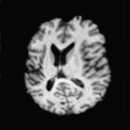
Figure 6: Image I16subscript𝐼16I_{1-6}
Refer to caption
(a) I1subscript𝐼1I_{1}
Refer to caption
(b) I2subscript𝐼2I_{2}
Refer to caption
(c) I3subscript𝐼3I_{3}
Refer to caption
(d) I4subscript𝐼4I_{4}
Refer to caption
(e) I5subscript𝐼5I_{5}
Refer to caption
(f) I6subscript𝐼6I_{6}

Now when we take f0=16i6J(𝑫i)1subscript𝑓016superscriptsubscript𝑖6𝐽subscript𝑫𝑖1f_{0}=\frac{1}{6}\sum_{i}^{6}{J(\boldsymbol{D}_{i})}\approx 1 and g0=16i6curl(𝑫i)0subscript𝑔016superscriptsubscript𝑖6curlsubscript𝑫𝑖0g_{0}=\frac{1}{6}\ \sum_{i}^{6}{\text{curl}(\boldsymbol{D}_{i})}\ \approx 0, by the Variational Principle, the average of these images is expected to be a good approximation to GT. We will verify this in Example 3. The Sum of Squared Differences (SSD)𝑆𝑆𝐷(SSD) between Iisubscript𝐼𝑖I_{i} and GT — SSD(Ii,I0)𝑆𝑆𝐷subscript𝐼𝑖subscript𝐼0SSD(I_{i},I_{0}) (they can be seen as the initial difference from Iisubscript𝐼𝑖I_{i} to I0subscript𝐼0I_{0}) are shown in the following table:

i𝑖i 111 222 333 444 555 666
SSD(Ii,I0)=(106)SSD(I_{i},I_{0})=(10^{6})* 1.8923 1.8906 1.8986 1.9610 1.8309 1.8353

Example 3: General Approach

In this example, we will walk through our method for the construction of unbiased template in a general sense. Step 1: take one image Iisubscript𝐼𝑖I_{i} out of the six images as the initial template, then register Iisubscript𝐼𝑖I_{i} to all six images Ijsubscript𝐼𝑗I_{j} for j=1,2,,6𝑗126j=1,2,\dots,6 (arrowed dash-lines) to find six registration transformations — ϕijsubscriptbold-italic-ϕ𝑖𝑗\boldsymbol{\phi}_{ij} for j=1,2,,6𝑗126j=1,2,\dots,6; Step 2: find the average transformation 𝒂𝒗𝒈i=avg(ϕij=1,,6)𝒂𝒗subscript𝒈𝑖𝑎𝑣𝑔subscriptbold-italic-ϕ𝑖𝑗16\boldsymbol{avg}_{i}=avg(\boldsymbol{\phi}_{ij=1,\dots,6}) of the six registration deformations by the Variational Principle (arrowed solid-line), as are demonstrated in the following diagram.

I1subscript𝐼1I_{1} I2subscript𝐼2I_{2} I3subscript𝐼3I_{3} I4subscript𝐼4I_{4} I5subscript𝐼5I_{5} I6subscript𝐼6I_{6} ϕi1subscriptbold-italic-ϕ𝑖1\boldsymbol{\phi}_{i1}ϕi2subscriptbold-italic-ϕ𝑖2\boldsymbol{\phi}_{i2}ϕi3subscriptbold-italic-ϕ𝑖3\boldsymbol{\phi}_{i3}ϕi4subscriptbold-italic-ϕ𝑖4\boldsymbol{\phi}_{i4}ϕi5subscriptbold-italic-ϕ𝑖5\boldsymbol{\phi}_{i5}ϕi6subscriptbold-italic-ϕ𝑖6\boldsymbol{\phi}_{i6}𝒂𝒗𝒈i𝒂𝒗subscript𝒈𝑖\boldsymbol{avg}_{i} Iisubscript𝐼𝑖I_{i} (initial template)

Step 3, re-sample Iisubscript𝐼𝑖I_{i} on the average transformation 𝒂𝒗𝒈i𝒂𝒗subscript𝒈𝑖\boldsymbol{avg}_{i}, indicated as the next diagram and shown in Figure 7, to get the biased temporary templates T^emplatei=Ii(𝒂𝒗𝒈i)^𝑇𝑒𝑚𝑝𝑙𝑎𝑡subscript𝑒𝑖subscript𝐼𝑖𝒂𝒗subscript𝒈𝑖{\hat{T}emplate}_{i}=I_{i}(\boldsymbol{avg}_{i}) for each i=1,2,,6𝑖126i=1,2,\dots,6 which are shown in Figure 8.

Iisubscript𝐼𝑖I_{i} (initial template) 𝒂𝒗𝒈i𝒂𝒗subscript𝒈𝑖\boldsymbol{avg}_{i} T^emplatei^𝑇𝑒𝑚𝑝𝑙𝑎𝑡subscript𝑒𝑖{\hat{T}emplate}_{i}
Figure 7: Average transformation — 𝒂𝒗𝒈i=avg(ϕij=1,,6)𝒂𝒗subscript𝒈𝑖𝑎𝑣𝑔subscriptbold-italic-ϕ𝑖𝑗16\boldsymbol{avg}_{i}=avg(\boldsymbol{\phi}_{ij=1,\dots,6})
Refer to caption
(a) 𝒂𝒗𝒈1𝒂𝒗subscript𝒈1\boldsymbol{avg}_{1}
Refer to caption
(b) 𝒂𝒗𝒈2𝒂𝒗subscript𝒈2\boldsymbol{avg}_{2}
Refer to caption
(c) 𝒂𝒗𝒈3𝒂𝒗subscript𝒈3\boldsymbol{avg}_{3}
Refer to caption
(d) 𝒂𝒗𝒈4𝒂𝒗subscript𝒈4\boldsymbol{avg}_{4}
Refer to caption
(e) 𝒂𝒗𝒈5𝒂𝒗subscript𝒈5\boldsymbol{avg}_{5}
Refer to caption
(f) 𝒂𝒗𝒈6𝒂𝒗subscript𝒈6\boldsymbol{avg}_{6}
Figure 8: Biased Temporary Templates — T^emplatei=Ii(𝒂𝒗𝒈i)^𝑇𝑒𝑚𝑝𝑙𝑎𝑡subscript𝑒𝑖subscript𝐼𝑖𝒂𝒗subscript𝒈𝑖\hat{T}emplate_{i}=I_{i}(\boldsymbol{avg}_{i})
Refer to caption
(a) T^emplate1^𝑇𝑒𝑚𝑝𝑙𝑎𝑡subscript𝑒1\hat{T}emplate_{1}
Refer to caption
(b) T^emplate2^𝑇𝑒𝑚𝑝𝑙𝑎𝑡subscript𝑒2\hat{T}emplate_{2}
Refer to caption
(c) T^emplate3^𝑇𝑒𝑚𝑝𝑙𝑎𝑡subscript𝑒3\hat{T}emplate_{3}
Refer to caption
(d) T^emplate4^𝑇𝑒𝑚𝑝𝑙𝑎𝑡subscript𝑒4\hat{T}emplate_{4}
Refer to caption
(e) T^emplate5^𝑇𝑒𝑚𝑝𝑙𝑎𝑡subscript𝑒5\hat{T}emplate_{5}
Refer to caption
(f) T^emplate6^𝑇𝑒𝑚𝑝𝑙𝑎𝑡subscript𝑒6\hat{T}emplate_{6}

The SSD between I^isubscript^𝐼𝑖\hat{I}_{i} with the GT — SSD(T^emplatei,I0)𝑆𝑆𝐷^𝑇𝑒𝑚𝑝𝑙𝑎𝑡subscript𝑒𝑖subscript𝐼0SSD({\hat{T}emplate}_{i},I_{0}) and Errori=SSD(T^emplatei,I0)SSD(Ii,I0)𝐸𝑟𝑟𝑜subscript𝑟𝑖𝑆𝑆𝐷^𝑇𝑒𝑚𝑝𝑙𝑎𝑡subscript𝑒𝑖subscript𝐼0𝑆𝑆𝐷subscript𝐼𝑖subscript𝐼0Error_{i}=\frac{SSD({\hat{T}emplate}_{i},I_{0})}{SSD(I_{i},I_{0})} are shown in the following table. Errori𝐸𝑟𝑟𝑜subscript𝑟𝑖Error_{i} measures the error reduction in temporary template T^emplatei^𝑇𝑒𝑚𝑝𝑙𝑎𝑡subscript𝑒𝑖{\hat{T}emplate}_{i} compared to the image Iisubscript𝐼𝑖I_{i}.

i𝑖i 111 222 333 444 555 666
SSD(T^emplatei,I0)=(106)SSD(\hat{T}emplate_{i},I_{0})=(10^{6})* 2.0504 3.4073 0.4963 0.4905 0.4835 0.5116
Errori𝐸𝑟𝑟𝑜subscript𝑟𝑖Error_{i} 0.1084 0.1802 0.0261 0.0250 0.0264 0.0279

As it can be seen, T^emplate2^𝑇𝑒𝑚𝑝𝑙𝑎𝑡subscript𝑒2{\hat{T}emplate}_{2} has the highest error =0.1802absent0.1802=0.1802. At this stage, T^emplate4^𝑇𝑒𝑚𝑝𝑙𝑎𝑡subscript𝑒4{\hat{T}emplate}_{4} is the best with an error 0.0250 (this means 97.5%percent97.597.5\% of the initial SSD𝑆𝑆𝐷SSD between image I4subscript𝐼4I_{4} and GT is reduced by our optimal control registration method). The large difference between Error2=0.1802𝐸𝑟𝑟𝑜subscript𝑟20.1802Error_{2}=0.1802 and Error4=0.0250𝐸𝑟𝑟𝑜subscript𝑟40.0250Error_{4}=0.0250 indicates the existence of bias towards the image that is used as an initial template. In order to quantify the bias, we calculate the sample mean and standard deviation of the six SSD(T^emplatei,I0)𝑆𝑆𝐷^𝑇𝑒𝑚𝑝𝑙𝑎𝑡subscript𝑒𝑖subscript𝐼0SSD({\hat{T}emplate}_{i},I_{0})’s: Sample Mean =1.2400(106)absent1.2400superscript106=1.2400*(10^{6}), Sample Standard Deviation =1.2306(106)absent1.2306superscript106=1.2306*(10^{6}). So, SSD(T^emplate6,I0)𝑆𝑆𝐷^𝑇𝑒𝑚𝑝𝑙𝑎𝑡subscript𝑒6subscript𝐼0SSD(\hat{T}emplate_{6},I_{0}) is the closest to the Sample Mean. But the large standard deviation of this sample disqualifies any one of these templates as unbiased.

This leads to Step-4: repeat Step-1 to Step-3 on biased temporary templates — T^emplatei^𝑇𝑒𝑚𝑝𝑙𝑎𝑡subscript𝑒𝑖\hat{T}emplate_{i} to reduce their bias. So we get a new group of average transformation 𝑨𝒗𝒈i𝑨𝒗subscript𝒈𝑖\boldsymbol{Avg}_{i} as shown in Figure 9 and the re-sampled images are the Unbiased Templates — Templatei=T^emplatei(𝑨𝒗𝒈i)𝑇𝑒𝑚𝑝𝑙𝑎𝑡subscript𝑒𝑖^𝑇𝑒𝑚𝑝𝑙𝑎𝑡subscript𝑒𝑖𝑨𝒗subscript𝒈𝑖Template_{i}=\hat{T}emplate_{i}(\boldsymbol{Avg}_{i}) as shown in Figure 10.

Figure 9: Average transformation — 𝑨𝒗𝒈i𝑨𝒗subscript𝒈𝑖\boldsymbol{Avg}_{i}
Refer to caption
(a) 𝑨𝒗𝒈1𝑨𝒗subscript𝒈1\boldsymbol{Avg}_{1}
Refer to caption
(b) 𝑨𝒗𝒈2𝑨𝒗subscript𝒈2\boldsymbol{Avg}_{2}
Refer to caption
(c) 𝑨𝒗𝒈3𝑨𝒗subscript𝒈3\boldsymbol{Avg}_{3}
Refer to caption
(d) 𝑨𝒗𝒈4𝑨𝒗subscript𝒈4\boldsymbol{Avg}_{4}
Refer to caption
(e) 𝑨𝒗𝒈5𝑨𝒗subscript𝒈5\boldsymbol{Avg}_{5}
Refer to caption
(f) 𝑨𝒗𝒈6𝑨𝒗subscript𝒈6\boldsymbol{Avg}_{6}
Figure 10: Unbiased Templates — Templatei=T^emplatei(𝑨𝒗𝒈i)𝑇𝑒𝑚𝑝𝑙𝑎𝑡subscript𝑒𝑖^𝑇𝑒𝑚𝑝𝑙𝑎𝑡subscript𝑒𝑖𝑨𝒗subscript𝒈𝑖Template_{i}=\hat{T}emplate_{i}(\boldsymbol{Avg}_{i})
Refer to caption
(a) Template1𝑇𝑒𝑚𝑝𝑙𝑎𝑡subscript𝑒1Template_{1}
Refer to caption
(b) Template2𝑇𝑒𝑚𝑝𝑙𝑎𝑡subscript𝑒2Template_{2}
Refer to caption
(c) Template3𝑇𝑒𝑚𝑝𝑙𝑎𝑡subscript𝑒3Template_{3}
Refer to caption
(d) Template4𝑇𝑒𝑚𝑝𝑙𝑎𝑡subscript𝑒4Template_{4}
Refer to caption
(e) Template5𝑇𝑒𝑚𝑝𝑙𝑎𝑡subscript𝑒5Template_{5}
Refer to caption
(f) Template6𝑇𝑒𝑚𝑝𝑙𝑎𝑡subscript𝑒6Template_{6}

The SSD between Templatei𝑇𝑒𝑚𝑝𝑙𝑎𝑡subscript𝑒𝑖Template_{i} with the GT — SSD(Templatei,I0)𝑆𝑆𝐷𝑇𝑒𝑚𝑝𝑙𝑎𝑡subscript𝑒𝑖subscript𝐼0SSD({Template}_{i},I_{0}) and Errori=SSD(Templatei,I0)SSD(Ii,I0)𝐸𝑟𝑟𝑜subscript𝑟𝑖𝑆𝑆𝐷𝑇𝑒𝑚𝑝𝑙𝑎𝑡subscript𝑒𝑖subscript𝐼0𝑆𝑆𝐷subscript𝐼𝑖subscript𝐼0Error_{i}=\frac{SSD({Template}_{i},I_{0})}{SSD(I_{i},I_{0})} are shown in the following table which measures the error reduction in temporary template Templatei𝑇𝑒𝑚𝑝𝑙𝑎𝑡subscript𝑒𝑖{Template}_{i} compared to the image Iisubscript𝐼𝑖I_{i}.

i𝑖i 111 222 333 444 555 666
SSD(Templatei,I0)=(105)SSD(Template_{i},I_{0})=(10^{5})* 6.7786 6.6041 5.5583 5.6649 5.7469 5.8088
Errori𝐸𝑟𝑟𝑜subscript𝑟𝑖Error_{i} 0.0358 0.0349 0.0292 0.0289 0.0314 0.0317

The statistics are significantly improved: New Sample Mean =6.0269(105)absent6.0269superscript105=6.0269*(10^{5}); New Sample Standard Deviation =5.2436(104)absent5.2436superscript104=5.2436*(10^{4}). Template6𝑇𝑒𝑚𝑝𝑙𝑎𝑡subscript𝑒6Template_{6} is closest to the New Sample Mean. The New Sample Standard Deviation =5.2436(104)absent5.2436superscript104=5.2436*(10^{4}) is now only 4.3566%percent4.35664.3566\% of the previous Sample Standard Deviation =1.2306(106)absent1.2306superscript106=1.2306*(10^{6}). This means, the effectiveness of repeating Step-1 to Step-3 on the biased temporary templates has greatly reduced the bias of biased tmporary template {T^emplatei}^𝑇𝑒𝑚𝑝𝑙𝑎𝑡subscript𝑒𝑖\{\hat{T}emplate_{i}\}. Hence, we can take any of the new templates Templatei𝑇𝑒𝑚𝑝𝑙𝑎𝑡subscript𝑒𝑖Template_{i} as an unbiased template. To check that, we may register each of Templatei𝑇𝑒𝑚𝑝𝑙𝑎𝑡subscript𝑒𝑖Template_{i} to I0subscript𝐼0I_{0} to get six register transformations and all of them are expected to be close to the identity map 𝑰𝒅𝑰𝒅\boldsymbol{Id} as the results are shown in Figure 11.

Figure 11: Average transformation — 𝑰^𝒅ibold-^𝑰subscript𝒅𝑖\boldsymbol{\hat{I}d}_{i}
Refer to caption
(a) 𝑰^𝒅1bold-^𝑰subscript𝒅1\boldsymbol{\hat{I}d}_{1}
Refer to caption
(b) 𝑰^𝒅2bold-^𝑰subscript𝒅2\boldsymbol{\hat{I}d}_{2}
Refer to caption
(c) 𝑰^𝒅3bold-^𝑰subscript𝒅3\boldsymbol{\hat{I}d}_{3}
Refer to caption
(d) 𝑰^𝒅4bold-^𝑰subscript𝒅4\boldsymbol{\hat{I}d}_{4}
Refer to caption
(e) 𝑰^𝒅5bold-^𝑰subscript𝒅5\boldsymbol{\hat{I}d}_{5}
Refer to caption
(f) 𝑰^𝒅6bold-^𝑰subscript𝒅6\boldsymbol{\hat{I}d}_{6}

And the behaviors of their Jacobian determinant and curl are shown in the following table.

i𝑖i 111 222 333 444 555 666
max J(𝑰^𝒅i)𝐽bold-^𝑰subscript𝒅𝑖J(\boldsymbol{\hat{I}d}_{i}) 1.0000 1.0000 1.0000 1.0000 1.0000 1.0000
min J(𝑰^𝒅i)𝐽bold-^𝑰subscript𝒅𝑖J(\boldsymbol{\hat{I}d}_{i}) 0.9999 0.9999 0.9999 0.9999 0.9999 0.9999
max curl(𝑰^𝒅i)=1014\text{curl}(\boldsymbol{\hat{I}d}_{i})=10^{-14}* 0.3553 0.3553 0.1776 0.1776 0.3553 0.3553
min curl(𝑰^𝒅i)=1014\text{curl}(\boldsymbol{\hat{I}d}_{i})=10^{-14}* -0.3553 -0.3553 -0.1776 -0.1776 -0.3553 -0.3553

Example 4: Computation Friendly Approach

In Example 3, the crucial part is Step-3 for our general approach of constructing an unbiased template, which requires to find all T^emplatei^𝑇𝑒𝑚𝑝𝑙𝑎𝑡subscript𝑒𝑖\hat{T}emplate_{i} for all i=1,,6𝑖16i=1,\dots,6 and it is not a cheap task to do in terms of computational costs. In this example, we construct a correction transformation to reduce the bias of any initial template Iisubscript𝐼𝑖I_{i}, by using an approximation to composition of small deformations, which “allows” us to do a similar job without finding all T^emplatei^𝑇𝑒𝑚𝑝𝑙𝑎𝑡subscript𝑒𝑖\hat{T}emplate_{i}. This can be done under the assumption that ground-truth Jacobian determinant and curl-vector are known.

Let’s take one of the Iisubscript𝐼𝑖I_{i} as the initial template, then we perform Step-1 and Step-2 as they were in Example 3, to get an biased temporary template T^emplatei^𝑇𝑒𝑚𝑝𝑙𝑎𝑡subscript𝑒𝑖\hat{T}emplate_{i}. To see the process is independent of choosing initial template, we will show the results of all six image Iisubscript𝐼𝑖I_{i} as the initial template individually.

Correction transformation 𝑯isubscript𝑯𝑖\boldsymbol{H}_{i}’s

We have derived a mathematical formula to generate correction transformations 𝑯isubscript𝑯𝑖\boldsymbol{H}_{i}’s for each of T^emplatei^𝑇𝑒𝑚𝑝𝑙𝑎𝑡subscript𝑒𝑖\hat{T}emplate_{i} where i=1,,6𝑖16i=1,\dots,6. Let {Ii}subscript𝐼𝑖\{I_{i}\} be the given images and {T^emplatei}^𝑇𝑒𝑚𝑝𝑙𝑎𝑡subscript𝑒𝑖\{{\hat{T}emplate}_{i}\} be the temporary templates by above procedures. As it can be seen in Example 3, using I1subscript𝐼1I_{1} and I2subscript𝐼2I_{2} to form the temporary templates would give strongly biased results. Therefore, in order to construct unbiased template, a correction transformation 𝑯isubscript𝑯𝑖\boldsymbol{H}_{i} needs to be introduced which depends on the initial template Iisubscript𝐼𝑖I_{i}.

To construct 𝑯isubscript𝑯𝑖\boldsymbol{H}_{i}(arrowed solid-line on the diagram) for a fixed i𝑖i: Firstly, applying our image registration method to find registration transformations ϕ^ij:T^emplateiIj:subscript^bold-italic-ϕ𝑖𝑗^𝑇𝑒𝑚𝑝𝑙𝑎𝑡subscript𝑒𝑖subscript𝐼𝑗\hat{\boldsymbol{\phi}}_{ij}:{\hat{T}emplate}_{i}\longrightarrow I_{j}, for-all\forall j=1,2,N𝑗12𝑁j=1,2...,N (arrowed dash-line on the diagram). Let consider the following diagram:

I1subscript𝐼1I_{1} I2subscript𝐼2I_{2} I3subscript𝐼3I_{3} I4subscript𝐼4I_{4} I5subscript𝐼5I_{5} I6subscript𝐼6I_{6} ϕ^i1subscriptbold-^bold-italic-ϕ𝑖1\boldsymbol{\hat{\phi}}_{i1}ϕ^i2subscriptbold-^bold-italic-ϕ𝑖2\boldsymbol{\hat{\phi}}_{i2}ϕ^i3subscriptbold-^bold-italic-ϕ𝑖3\boldsymbol{\hat{\phi}}_{i3}ϕ^i4subscriptbold-^bold-italic-ϕ𝑖4\boldsymbol{\hat{\phi}}_{i4}ϕ^i5subscriptbold-^bold-italic-ϕ𝑖5\boldsymbol{\hat{\phi}}_{i5}ϕ^i6subscriptbold-^bold-italic-ϕ𝑖6\boldsymbol{\hat{\phi}}_{i6} T^emplatei^𝑇𝑒𝑚𝑝𝑙𝑎𝑡subscript𝑒𝑖\hat{T}emplate_{i} 𝑯isubscript𝑯𝑖\boldsymbol{H}_{i} Templatei𝑇𝑒𝑚𝑝𝑙𝑎𝑡subscript𝑒𝑖Template_{i}

The construction of biased temporary templates T^emplatei^𝑇𝑒𝑚𝑝𝑙𝑎𝑡subscript𝑒𝑖\hat{T}emplate_{i} are actually expected to be the unbiased template Templatei𝑇𝑒𝑚𝑝𝑙𝑎𝑡subscript𝑒𝑖Template_{i} in Step-1 and Step-2 of Example 3. Due to computational limitations, they did not reduce the bias enough, so we got only a biased temporary template T^emplatei^𝑇𝑒𝑚𝑝𝑙𝑎𝑡subscript𝑒𝑖\hat{T}emplate_{i}. However, the original bias of the initial template Iisubscript𝐼𝑖I_{i} has been reduced to a level that makes the temporary templates T^emplatei^𝑇𝑒𝑚𝑝𝑙𝑎𝑡subscript𝑒𝑖\hat{T}emplate_{i} closer to I0subscript𝐼0I_{0} than the initial template Iisubscript𝐼𝑖I_{i}. We would like to ask, does it exist a small deformation 𝑯i(𝒙)subscript𝑯𝑖𝒙\boldsymbol{H}_{i}(\boldsymbol{x}) that deforms the unbiased template Templatei𝑇𝑒𝑚𝑝𝑙𝑎𝑡subscript𝑒𝑖Template_{i} to T^emplatei^𝑇𝑒𝑚𝑝𝑙𝑎𝑡subscript𝑒𝑖\hat{T}emplate_{i}? If it exists, how to find it?

Secondly, according to our definition of unbiased template, if 𝑯isubscript𝑯𝑖\boldsymbol{H}_{i} exists, then it must satisfy the following equations:

{j=1NJ(ϕ^ij𝑯i(𝒙))N=1j=1Ncurl(ϕ^ij𝑯i(𝒙))=0\left\{\begin{aligned} \frac{\sum_{j=1}^{N}J(\hat{\boldsymbol{\phi}}_{ij}\circ\boldsymbol{H}_{i}(\boldsymbol{x}))}{N}&=1\\ \sum_{j=1}^{N}\text{curl}(\hat{\boldsymbol{\phi}}_{ij}\circ\boldsymbol{H}_{i}(\boldsymbol{x}))&=0\end{aligned}\right. (3.1)

This means, if there exists an unbiased template which should be almost identical to GT — I0subscript𝐼0I_{0}, then the each compositions of ϕ^ij𝑯isubscript^bold-italic-ϕ𝑖𝑗subscript𝑯𝑖\hat{\boldsymbol{\phi}}_{ij}\circ\boldsymbol{H}_{i} should behaves very close to the inverse transformation of 𝑫isubscript𝑫𝑖\boldsymbol{D}_{i}, where 𝑫isubscript𝑫𝑖\boldsymbol{D}_{i} were shown in Figure 5. Therefore the average of J(ϕ^ij𝑯i(𝒙))𝐽subscript^bold-italic-ϕ𝑖𝑗subscript𝑯𝑖𝒙J(\hat{\boldsymbol{\phi}}_{ij}\circ\boldsymbol{H}_{i}(\boldsymbol{x})) should be 111 and the average curl(ϕ^ij𝑯i(𝒙))curlsubscript^bold-italic-ϕ𝑖𝑗subscript𝑯𝑖𝒙\text{curl}(\hat{\boldsymbol{\phi}}_{ij}\circ\boldsymbol{H}_{i}(\boldsymbol{x})) should be 00 for each i𝑖i.

By property J(𝑻2𝑻1)=J(𝑻1)J(𝑻2)𝐽subscript𝑻2subscript𝑻1𝐽subscript𝑻1𝐽subscript𝑻2J(\boldsymbol{T}_{2}\circ\boldsymbol{T}_{1})=J(\boldsymbol{T}_{1})J(\boldsymbol{T}_{2}), we know

j=1NJ(ϕ^ij𝑯i(𝒙))N=J(𝑯i(𝒙))j=1NJ(ϕ^ij(𝒙))N=1J(𝑯i(𝒙))=Nj=1NJ(ϕ^ij(𝒙))formulae-sequencesuperscriptsubscript𝑗1𝑁𝐽subscript^bold-italic-ϕ𝑖𝑗subscript𝑯𝑖𝒙𝑁𝐽subscript𝑯𝑖𝒙superscriptsubscript𝑗1𝑁𝐽subscript^bold-italic-ϕ𝑖𝑗𝒙𝑁1𝐽subscript𝑯𝑖𝒙𝑁superscriptsubscript𝑗1𝑁𝐽subscript^bold-italic-ϕ𝑖𝑗𝒙\frac{\sum_{j=1}^{N}J(\hat{\boldsymbol{\phi}}_{ij}\circ\boldsymbol{H}_{i}(\boldsymbol{x}))}{N}=J(\boldsymbol{H}_{i}(\boldsymbol{x}))\frac{\sum_{j=1}^{N}J(\hat{\boldsymbol{\phi}}_{ij}(\boldsymbol{x}))}{N}=1\hskip 28.45274pt\Longrightarrow\hskip 28.45274ptJ(\boldsymbol{H}_{i}(\boldsymbol{x}))=\frac{N}{\sum_{j=1}^{N}J(\hat{\boldsymbol{\phi}}_{ij}(\boldsymbol{x}))} (3.2)

𝑯i(𝒙)subscript𝑯𝑖𝒙\boldsymbol{H}_{i}(\boldsymbol{x}) is small deformation and it can be represented as 𝑯i(𝒙)=𝒙+𝒖i(𝒙)subscript𝑯𝑖𝒙𝒙subscript𝒖𝑖𝒙\boldsymbol{H}_{i}(\boldsymbol{x})=\boldsymbol{x}+\boldsymbol{u}_{i}(\boldsymbol{x}), therefore, we have

curl(𝑯i(𝒙))=curl(𝒖i(𝒙))curlsubscript𝑯𝑖𝒙curlsubscript𝒖𝑖𝒙\text{curl}(\boldsymbol{H}_{i}(\boldsymbol{x}))=\text{curl}(\boldsymbol{u}_{i}(\boldsymbol{x})) (3.3)

And composition of two small deformations, let 𝑻1(𝒙)=𝒙+𝒖1(𝒙)subscript𝑻1𝒙𝒙subscript𝒖1𝒙\boldsymbol{T}_{1}(\boldsymbol{x})=\boldsymbol{x}+\boldsymbol{u}_{1}(\boldsymbol{x}) and 𝑻2(𝒙)=𝒙+𝒖2(𝒙)subscript𝑻2𝒙𝒙subscript𝒖2𝒙\boldsymbol{T}_{2}(\boldsymbol{x})=\boldsymbol{x}+\boldsymbol{u}_{2}(\boldsymbol{x}) where 𝒖i(𝒙)subscript𝒖𝑖𝒙\boldsymbol{u}_{i}(\boldsymbol{x}) are displacement fields, can be approximated [5] by

𝑻2𝑻1(𝒙)𝒙+𝒖1(𝒙)+𝒖2(𝒙)=𝒙+𝒖2(𝒙)+𝒖1(𝒙)=𝑻2(𝒙)+𝒖1(𝒙)subscript𝑻2subscript𝑻1𝒙𝒙subscript𝒖1𝒙subscript𝒖2𝒙𝒙subscript𝒖2𝒙subscript𝒖1𝒙subscript𝑻2𝒙subscript𝒖1𝒙\boldsymbol{T}_{2}\circ\boldsymbol{T}_{1}(\boldsymbol{x})\approx\boldsymbol{x}+\boldsymbol{u}_{1}(\boldsymbol{x})+\boldsymbol{u}_{2}(\boldsymbol{x})=\boldsymbol{x}+\boldsymbol{u}_{2}(\boldsymbol{x})+\boldsymbol{u}_{1}(\boldsymbol{x})=\boldsymbol{T}_{2}(\boldsymbol{x})+\boldsymbol{u}_{1}(\boldsymbol{x})

this leads to

𝑯iϕ^ij(𝒙)ϕ^ij(𝒙)+𝒖i(𝒙)subscript𝑯𝑖subscript^bold-italic-ϕ𝑖𝑗𝒙subscript^bold-italic-ϕ𝑖𝑗𝒙subscript𝒖𝑖𝒙\boldsymbol{H}_{i}\circ\hat{\boldsymbol{\phi}}_{ij}(\boldsymbol{x})\approx\hat{\boldsymbol{\phi}}_{ij}(\boldsymbol{x})+\boldsymbol{u}_{i}(\boldsymbol{x})

Therefore, by (3.3), we have

curl(𝑯iϕ^ij(𝒙))curl(ϕ^ij)+curl(𝒖i(𝒙))=curl(ϕ^ij)+curl(𝑯i(𝒙))curlsubscript𝑯𝑖subscript^bold-italic-ϕ𝑖𝑗𝒙curlsubscript^bold-italic-ϕ𝑖𝑗curlsubscript𝒖𝑖𝒙curlsubscript^bold-italic-ϕ𝑖𝑗curlsubscript𝑯𝑖𝒙\text{curl}(\boldsymbol{H}_{i}\circ\hat{\boldsymbol{\phi}}_{ij}(\boldsymbol{x}))\approx\text{curl}(\hat{\boldsymbol{\phi}}_{ij})+\text{curl}(\boldsymbol{u}_{i}(\boldsymbol{x}))=\text{curl}(\hat{\boldsymbol{\phi}}_{ij})+\text{curl}(\boldsymbol{H}_{i}(\boldsymbol{x})) (3.4)

Now, by (3.2) and (3.4), the approximations of Jacobian determinant and curl of 𝑯isubscript𝑯𝑖\boldsymbol{H}_{i} in (3.1), denoted as J(𝑯^i(𝒙))𝐽subscript^𝑯𝑖𝒙J(\hat{\boldsymbol{H}}_{i}(\boldsymbol{x})) and curl(𝑯^i(𝒙))curlsubscript^𝑯𝑖𝒙\text{curl}(\hat{\boldsymbol{H}}_{i}(\boldsymbol{x})), respectively, which are in the form of

{J(𝑯^i(𝒙))=Nj=1NJ(ϕ^ij(𝒙))curl(𝑯^i(𝒙))=j=1Ncurl(ϕ^ij(𝒙))N\left\{\begin{aligned} J(\hat{\boldsymbol{H}}_{i}(\boldsymbol{x}))&=\frac{N}{\sum_{j=1}^{N}J(\hat{\boldsymbol{\phi}}_{ij}(\boldsymbol{x}))}\\ \text{curl}(\hat{\boldsymbol{H}}_{i}(\boldsymbol{x}))&=\frac{-\sum_{j=1}^{N}\text{curl}(\hat{\boldsymbol{\phi}}_{ij}(\boldsymbol{x}))}{N}\end{aligned}\right. (3.5)

Finally, we find 𝑯^isubscript^𝑯𝑖\hat{\boldsymbol{H}}_{i} by our Variational Principle. The approximated transformations 𝑯^isubscript^𝑯𝑖\hat{\boldsymbol{H}}_{i}’s are shown in Figure 12.

Figure 12: Correction Transformation, 𝑯^16subscript^𝑯16\hat{\boldsymbol{H}}_{1-6}
Refer to caption
(a) 𝑯^1subscript^𝑯1\hat{\boldsymbol{H}}_{1}
Refer to caption
(b) 𝑯^2subscript^𝑯2\hat{\boldsymbol{H}}_{2}
Refer to caption
(c) 𝑯^3subscript^𝑯3\hat{\boldsymbol{H}}_{3}
Refer to caption
(d) 𝑯^4subscript^𝑯4\hat{\boldsymbol{H}}_{4}
Refer to caption
(e) 𝑯^5subscript^𝑯5\hat{\boldsymbol{H}}_{5}
Refer to caption
(f) 𝑯^6subscript^𝑯6\hat{\boldsymbol{H}}_{6}

After re-sampling each T^emplatei^𝑇𝑒𝑚𝑝𝑙𝑎𝑡subscript𝑒𝑖\hat{T}emplate_{i} on transformation 𝑯^isubscript^𝑯𝑖\hat{\boldsymbol{H}}_{i}’s, we obtain a set of six new templates Templatei𝑇𝑒𝑚𝑝𝑙𝑎𝑡subscript𝑒𝑖Template_{i} as shown in Figure 13, which are much more uniform now.

Figure 13: Unbiased Templates — Templatei𝑇𝑒𝑚𝑝𝑙𝑎𝑡subscript𝑒𝑖Template_{i}
Refer to caption
(a) Template1𝑇𝑒𝑚𝑝𝑙𝑎𝑡subscript𝑒1Template_{1}
Refer to caption
(b) Template2𝑇𝑒𝑚𝑝𝑙𝑎𝑡subscript𝑒2Template_{2}
Refer to caption
(c) Template3𝑇𝑒𝑚𝑝𝑙𝑎𝑡subscript𝑒3Template_{3}
Refer to caption
(d) Template4𝑇𝑒𝑚𝑝𝑙𝑎𝑡subscript𝑒4Template_{4}
Refer to caption
(e) Template5𝑇𝑒𝑚𝑝𝑙𝑎𝑡subscript𝑒5Template_{5}
Refer to caption
(f) Template6𝑇𝑒𝑚𝑝𝑙𝑎𝑡subscript𝑒6Template_{6}

Similarly as the results from Example 3, the highest error is 0.03720.03720.0372, downed from 0.18020.18020.1802. The SSD𝑆𝑆𝐷SSD between new templates Templatei𝑇𝑒𝑚𝑝𝑙𝑎𝑡subscript𝑒𝑖Template_{i}’s and I0subscript𝐼0I_{0} are reduced by an order of 101010 as SSD(Templatei,I0)𝑆𝑆𝐷𝑇𝑒𝑚𝑝𝑙𝑎𝑡subscript𝑒𝑖subscript𝐼0SSD(Template_{i},I_{0}) and Errori=SSD(Templatei,I0)SSD(Ii,I0)𝐸𝑟𝑟𝑜subscript𝑟𝑖𝑆𝑆𝐷𝑇𝑒𝑚𝑝𝑙𝑎𝑡subscript𝑒𝑖subscript𝐼0𝑆𝑆𝐷subscript𝐼𝑖subscript𝐼0Error_{i}=\frac{SSD(Template_{i},I_{0})}{SSD(I_{i},I_{0})} shown in the table. It measures the relative error in the new template Templatei𝑇𝑒𝑚𝑝𝑙𝑎𝑡subscript𝑒𝑖Template_{i} compared to the image Iisubscript𝐼𝑖I_{i}.

i𝑖i 111 222 333 444 555 666
SSD(Templatei,I0)=(105)SSD(Template_{i},I_{0})=(10^{5})* 6.6972 7.0447 5.0143 4.9911 5.0290 5.2408
Errori𝐸𝑟𝑟𝑜subscript𝑟𝑖Error_{i} 0.0354 0.0372 0.0264 0.0254 0.0274 0.0286

The statistics are also significantly improved just like in the results in Example 3: New Sample Mean =5.6695(105)absent5.6695superscript105=5.6695*(10^{5}); New Sample Standard Deviation =9.4137(104)absent9.4137superscript104=9.4137*(10^{4}). Template6𝑇𝑒𝑚𝑝𝑙𝑎𝑡subscript𝑒6Template_{6} is closest to the New Sample Mean. The New Sample Standard Deviation =9.4137(104)absent9.4137superscript104=9.4137*(10^{4}) is now only 7.65%percent7.657.65\% of the previous Sample Standard Deviation =1.2306(106)absent1.2306superscript106=1.2306*(10^{6}). This means, with the help of approximated correction transformations 𝑯^isubscript^𝑯𝑖\hat{\boldsymbol{H}}_{i}, we have greatly reduced the bias. And 𝑯^isubscript^𝑯𝑖\hat{\boldsymbol{H}}_{i} has been a good approximation to 𝑯isubscript𝑯𝑖\boldsymbol{H}_{i}. To check that, we registered Templatei𝑇𝑒𝑚𝑝𝑙𝑎𝑡subscript𝑒𝑖Template_{i} to I0subscript𝐼0I_{0} for each i𝑖i, denoted as 𝑰^𝒅ibold-^𝑰subscript𝒅𝑖\boldsymbol{\hat{I}d}_{i} which are shown in next Figure 14. They are expected to be close to the identity map 𝑰𝒅𝑰𝒅\boldsymbol{Id}. Therefore, we can take any of the new templates Templatei𝑇𝑒𝑚𝑝𝑙𝑎𝑡subscript𝑒𝑖Template_{i} as an unbiased template.

Figure 14: 𝑰^𝒅ibold-^𝑰subscript𝒅𝑖\boldsymbol{\hat{I}d}_{i}
Refer to caption
(a) 𝑰^𝒅1bold-^𝑰subscript𝒅1\boldsymbol{\hat{I}d}_{1}
Refer to caption
(b) 𝑰^𝒅2bold-^𝑰subscript𝒅2\boldsymbol{\hat{I}d}_{2}
Refer to caption
(c) 𝑰^𝒅3bold-^𝑰subscript𝒅3\boldsymbol{\hat{I}d}_{3}
Refer to caption
(d) 𝑰^𝒅4bold-^𝑰subscript𝒅4\boldsymbol{\hat{I}d}_{4}
Refer to caption
(e) 𝑰^𝒅5bold-^𝑰subscript𝒅5\boldsymbol{\hat{I}d}_{5}
Refer to caption
(f) 𝑰^𝒅6bold-^𝑰subscript𝒅6\boldsymbol{\hat{I}d}_{6}
i𝑖i 111 222 333 444 555 666
max J(𝑰^𝒅i)𝐽bold-^𝑰subscript𝒅𝑖J(\boldsymbol{\hat{I}d}_{i}) 1.0000 1.0000 1.0000 1.0000 1.0000 1.0000
min J(𝑰^𝒅i)𝐽bold-^𝑰subscript𝒅𝑖J(\boldsymbol{\hat{I}d}_{i}) 0.9999 0.9999 0.9999 0.9999 0.9999 0.9999
max curl(𝑰^𝒅i)=1014\text{curl}(\boldsymbol{\hat{I}d}_{i})=10^{-14}* 0.3553 0.3553 0.1776 0.1776 0.1776 0.1776
min curl(𝑰^𝒅i)=1014\text{curl}(\boldsymbol{\hat{I}d}_{i})=10^{-14}* -0.3553 -0.3553 -0.1776 -0.1776 -0.1776 -0.1776

4 Optimal Control Method for Non-rigid Image Registration

In this section, we describe the image registration method that we used to calculate the examples. Image registration is the process of establishing pixel (voxel) correspondence between two or more images so that certain similarity measure is maximized, or a dis-similarity measure (DS𝐷𝑆DS) is minimized. The images can be taken from the same individual at different posts and different times; or from different individuals. The images can also be in different modalities.

Over last decades, many sophisticated methods have been developed. Most of these methods regularize the ill-posed registration problem by various penalty terms that are either based on physical models or geometric considerations. The cost to be minimized is the sum of D𝐷DS and the regularizing term Reg: C=DS+αReg𝐶𝐷𝑆𝛼𝑅𝑒𝑔C=DS+\alpha Reg, where α𝛼\alpha is a parameter controlling the trade-off between the data term DS𝐷𝑆DS and the regularizing term Reg𝑅𝑒𝑔Reg. There are two issues with this framework:

  1. (1)

    the addition of the second term distorted the problem; For instance, the regularizing term changed the optimal transportation flow to be non-gradient flow.

  2. (2)

    The determination of the value of α𝛼\alpha is more like an art than science. If it is too large, the registration transformation becomes too smooth; while if it is too small the computation becomes unstable.

Some methods introduce regularization implicitly. For instance, the splines-based method minimizes DS𝐷𝑆DS on a coarse grid (say 8 by 8 pixels are represented in a grid cell) whose nodes are the control points for splines. After the new locations of the control points are determined, locations of the remaining pixels are interpolated by the splines formulas.

In [4, 6] we proposed an optimal control approach that has no explicit penalty terms (and hence no parameters). Instead, we minimize DS𝐷𝑆DS subject to the constraints [𝒖]=𝑭delimited-[]𝒖𝑭\mathcal{L}[\boldsymbol{u}]=\boldsymbol{F} with respect to the control function 𝑭𝑭\boldsymbol{F}. The registration transformation T is iteratively determined: at the k+1𝑘1k+1 step, 𝑻k+1(𝒙)=𝑻k(𝒙+𝒖k+1)superscript𝑻𝑘1𝒙superscript𝑻𝑘𝒙superscript𝒖𝑘1\boldsymbol{T}^{k+1}(\boldsymbol{x})=\boldsymbol{T}^{k}(\boldsymbol{x}+\boldsymbol{u}^{k+1}). \mathcal{L} is a partial differential operator providing regularity. For instance, in 2D, we can take div(𝒖)=F1div𝒖subscript𝐹1\text{div}(\boldsymbol{u})=F_{1}, and curl(𝒖)=F2curl𝒖subscript𝐹2\text{curl}(\boldsymbol{u})=F_{2}. Or we can simply take Δ𝒖=𝑭Δ𝒖𝑭\mathrm{\Delta}\boldsymbol{u}=\boldsymbol{F}. In the version described in [4], there is a mechanism that keeps the Jacobian determinant positive, which in turn assures that 𝑻𝑻\boldsymbol{T} is a diffeomorphism (invertible and smooth).

The optimal control approach is inspired by the success of fluid control algorithms. The variational problem is solved by the gradient decent method. As indicated in the survey paper [9], one could add a penalty term to DS𝐷𝑆DS for specific application with a small parameter value α𝛼\alpha in order to use prior knowledge. We now present a teapot example.

Example 5: Registration of 3D Teapot Images by Optimal Control Method

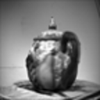
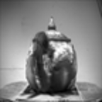
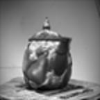
We now describe the volume image I0subscript𝐼0I_{0} and the twisted image Itsubscript𝐼𝑡I_{t} in Step-1. In Step-2, we register Itsubscript𝐼𝑡I_{t} to I0subscript𝐼0I_{0}, and out put the registration transformation and the deformed image Itsubscript𝐼𝑡I_{t}. The results show that the twisted image Itsubscript𝐼𝑡I_{t} is deformed back to the I0subscript𝐼0I_{0} with high accuracy.

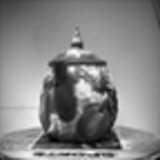
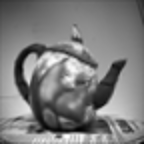
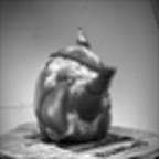
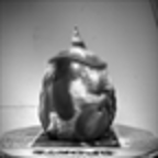
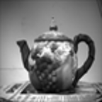
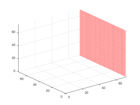
Step-1: A teapot is rotated about its vertical axis passing through the tip of its lid. Snapshots are taken from a fixed camera at 5superscript55^{\circ} intervals. A total of 72 photos are taken as the teapot completes 360superscript360360^{\circ} rotation and return to the initial position. Each of these photos is re-sampled as a 72×72727272\times 72 grayscale image I0isubscript𝐼0𝑖I_{0i}. These 72 images I0isubscript𝐼0𝑖I_{0i} for i=1,,72𝑖172i=1,\dots,72 are used to form a three dimensional volume image of size 72×72×7272727272\times 72\times 72. We refer to this volume image as the Rotating Teapot Image, denoted as I0subscript𝐼0I_{0}.

Figure 15: Teapot—I0subscript𝐼0I_{0}
Refer to caption
(a) 0superscript00^{\circ}
Refer to caption
(b) 45superscript4545^{\circ}
Refer to caption
(c) 90superscript9090^{\circ}
Refer to caption
(d) 135superscript135135^{\circ}
Refer to caption
(e) 180superscript180180^{\circ}
Refer to caption
(f) 225superscript225225^{\circ}
Refer to caption
(g) 270superscript270270^{\circ}
Refer to caption
(h) 315superscript315315^{\circ}
Refer to caption
(i) 360superscript360360^{\circ}

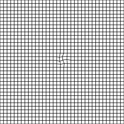
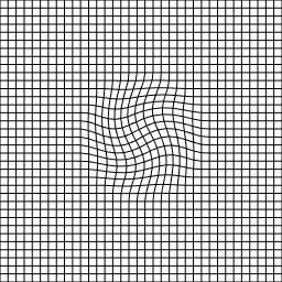
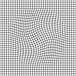
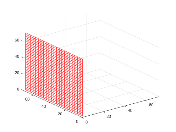
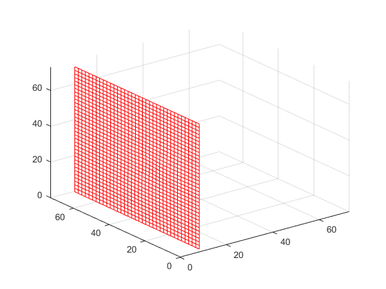
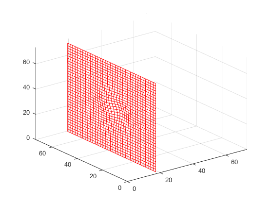
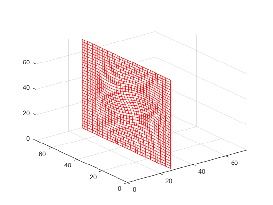
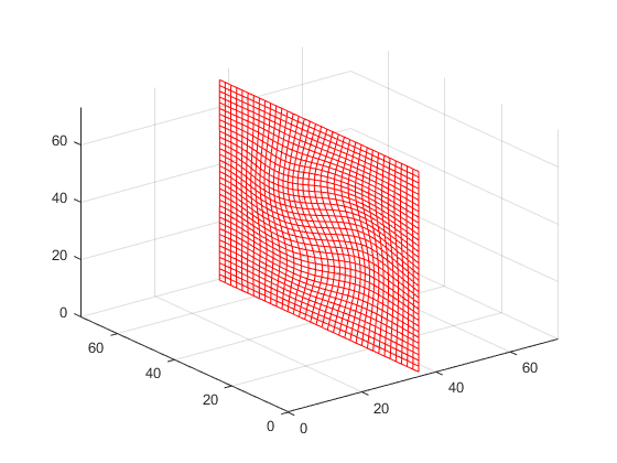
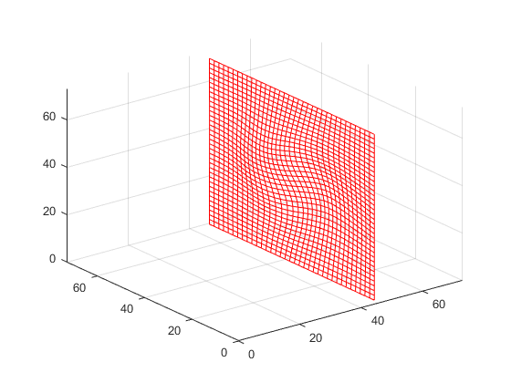
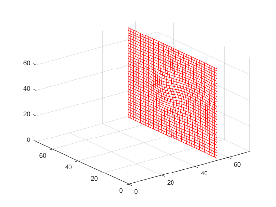
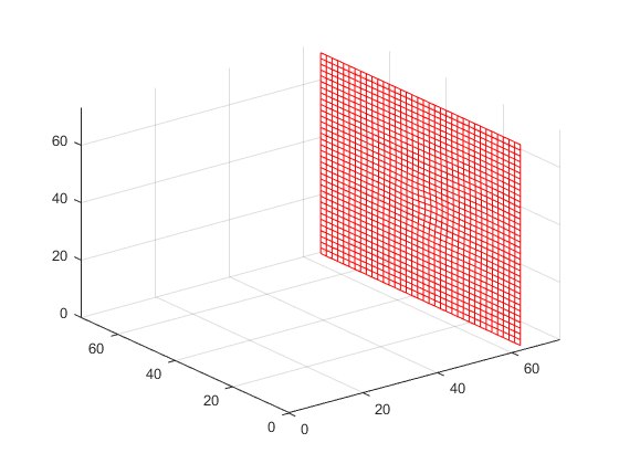
As the teapot rotates, we deform each slice I0isubscript𝐼0𝑖I_{0i} (of I0subscript𝐼0I_{0}) to Itisubscript𝐼𝑡𝑖I_{ti} by a rotation 𝑻isubscript𝑻𝑖\boldsymbol{T}_{i} as show in Figure 16 that is cut-off near the boundary for i=1,,72𝑖172i=1,\dots,72.

Figure 16: 𝑻isubscript𝑻𝑖\boldsymbol{T}_{i}’s
Refer to caption
(a) 𝑻1subscript𝑻1\boldsymbol{T}_{1}
Refer to caption
(b) 𝑻9subscript𝑻9\boldsymbol{T}_{9}
Refer to caption
(c) 𝑻18subscript𝑻18\boldsymbol{T}_{18}
Refer to caption
(d) 𝑻27subscript𝑻27\boldsymbol{T}_{27}
Refer to caption
(e) 𝑻36subscript𝑻36\boldsymbol{T}_{36}
Refer to caption
(f) 𝑻45subscript𝑻45\boldsymbol{T}_{45}
Refer to caption
(g) 𝑻54subscript𝑻54\boldsymbol{T}_{54}
Refer to caption
(h) 𝑻63subscript𝑻63\boldsymbol{T}_{63}
Refer to caption
(i) 𝑻72subscript𝑻72\boldsymbol{T}_{72}

These 72 twisted 72×72727272\times 72 images form a 72×72×7272727272\times 72\times 72 volume image referred to as the Twisted Teapot, denoted as Itsubscript𝐼𝑡I_{t} as shown in Figure 17.

Figure 17: Twisted Teapot—It=𝑻(I0)subscript𝐼𝑡𝑻subscript𝐼0I_{t}=\boldsymbol{T}(I_{0})
Refer to caption
(a) 0superscript00^{\circ}
Refer to caption
(b) 45superscript4545^{\circ}
Refer to caption
(c) 90superscript9090^{\circ}
Refer to caption
(d) 135superscript135135^{\circ}
Refer to caption
(e) 180superscript180180^{\circ}
Refer to caption
(f) 225superscript225225^{\circ}
Refer to caption
(g) 270superscript270270^{\circ}
Refer to caption
(h) 315superscript315315^{\circ}
Refer to caption
(i) 360superscript360360^{\circ}

The deformations 𝑻isubscript𝑻𝑖\boldsymbol{T}_{i} for i=1,,72𝑖172i=1,\dots,72 and the Twisted Teapot image Itsubscript𝐼𝑡I_{t} can be seen from Twisted Teapot(CLICK HERE)

Step-2: The registration transformation ϕbold-italic-ϕ\boldsymbol{\phi} from I0subscript𝐼0I_{0} to Itsubscript𝐼𝑡I_{t} is calculated by minimizing

SSD(ϕ(𝒙))=(It(ϕ(𝒙))I0(𝒙))2𝑑𝒙𝑆𝑆𝐷bold-italic-ϕ𝒙triple-integralsuperscriptsubscript𝐼𝑡bold-italic-ϕ𝒙subscript𝐼0𝒙2differential-d𝒙SSD(\boldsymbol{\phi}(\boldsymbol{x}))=\iiint(I_{t}(\boldsymbol{\phi}(\boldsymbol{x}))-I_{0}(\boldsymbol{x}))^{2}d\boldsymbol{x} (4.1)

The resulting registration deformation ϕbold-italic-ϕ\boldsymbol{\phi}, restricted to each i𝑖ith slice, is expected to be very close to 𝑻isubscript𝑻𝑖\boldsymbol{T}_{i} as shown in Figure 18.

Figure 18: ϕisubscriptbold-italic-ϕ𝑖\boldsymbol{\phi}_{i}’s
Refer to caption
(a) ϕ1subscriptbold-italic-ϕ1\boldsymbol{\phi}_{1}
Refer to caption
(b) ϕ9subscriptbold-italic-ϕ9\boldsymbol{\phi}_{9}
Refer to caption
(c) ϕ18subscriptbold-italic-ϕ18\boldsymbol{\phi}_{18}
Refer to caption
(d) ϕ27subscriptbold-italic-ϕ27\boldsymbol{\phi}_{27}
Refer to caption
(e) ϕ36subscriptbold-italic-ϕ36\boldsymbol{\phi}_{36}
Refer to caption
(f) ϕ45subscriptbold-italic-ϕ45\boldsymbol{\phi}_{45}
Refer to caption
(g) ϕ54subscriptbold-italic-ϕ54\boldsymbol{\phi}_{54}
Refer to caption
(h) ϕ63subscriptbold-italic-ϕ63\boldsymbol{\phi}_{63}
Refer to caption
(i) ϕ72subscriptbold-italic-ϕ72\boldsymbol{\phi}_{72}

and the deformed images of the twisted teapot — It(ϕ)subscript𝐼𝑡bold-italic-ϕI_{t}(\boldsymbol{\phi}) is expected to be close to I0subscript𝐼0I_{0} as it shows on next Figure 19. The total elapsed time for Step-2 is 927.601032 seconds.

Figure 19: Reversed Twisted Teapot—It(ϕ)subscript𝐼𝑡bold-italic-ϕI_{t}(\boldsymbol{\phi})
Refer to caption
(a) 0superscript00^{\circ}
Refer to caption
(b) 45superscript4545^{\circ}
Refer to caption
(c) 90superscript9090^{\circ}
Refer to caption
(d) 135superscript135135^{\circ}
Refer to caption
(e) 180superscript180180^{\circ}
Refer to caption
(f) 225superscript225225^{\circ}
Refer to caption
(g) 270superscript270270^{\circ}
Refer to caption
(h) 315superscript315315^{\circ}
Refer to caption
(i) 360superscript360360^{\circ}

The registration deformation ϕbold-italic-ϕ\boldsymbol{\phi} from Step-2 and the corresponding reversed twisted teapot image It=𝑻(I0)subscript𝐼𝑡𝑻subscript𝐼0I_{t}=\boldsymbol{T}(I_{0}) are shown from: Reversed Twisted Teapot(CLICK HERE). From these visualization files, we conclude that our optimal control method correctly recovered the ground truth deformations 𝑻isubscript𝑻𝑖\boldsymbol{T}_{i} for i=1,,72𝑖172i=1,\dots,72 and the grand truth images I0isubscript𝐼0𝑖I_{0i} for i=1,,72𝑖172i=1,\dots,72, as expected.

5 Conclusion

In this paper, a set of new computational techniques is described. They are based on both the Jacobian determinant and the curl-vector. Specifically, The Variational Principle is used to calculate a transformation with prescribed Jacobian determinant and curl-vector. A new method of averaging deformations based on averaging the Jacobian determinants and the curl-vectors is used to construct an unbiased template from the members of a set of images. We will further refine the techniques and generalize them to three dimensional real world images.

References

  • [1] Ashburner, J.: VBM Tutorial. http://www.fil.ion.ucl.ac.uk/ john/misc/VBMclass10.pdf, Mar 15, 2010.
  • [2] Ashburner, J and Friston, K. J.: COMMENTS AND CONTROVERSIES, Why Voxel-Based Morphometry Should Be Used. NeuroImage, Vol. 14, pp. 1238-1243, 2001. doi:10.1006/nimg.2001.0961
  • [3] Bookstein, F. L.: Voxel-Based Morphometry Should Not Be Used with Imperfectly Registered Images. NeuroImage, Vol. 14, Issue 6, pp. 1454-1462, 2001.
  • [4] Hsiao, H-Y., Hsieh, C-Y., Chen, X., Gong, Y., Luo, X. and Liao, G.: New Development of Nonrigid Registration. ANZIAM Journal, Vol. 55, pp. 289-297, 2014. doi:10.1017/S1446181114000091
  • [5] Hoshi, S., Davis, B., Jomier, M. and Gerig, G.:: Unbiased Diffeomorphic Atlas Construction for Computational Anatomy NeuroImage, Vol. 23, pp151-160, 2004. doi:10.1016/j.neuroimage.2004.07.068
  • [6] Liao, G., Cai, X., Fleitas, D., Luo, L., Wang, J. and Xue, J.: Optimal control approach to data set alignment Applied Mathematics Letters, Vol 21, pp. 898–905, 2008
  • [7] Narayana, P. A., Datta, S., Tao, G., Steinberg, J. L. and Moeller, F. G.: Effect of Cocaine on Structural Changes in Brain: MRI Volumetry using Tensor-Based Morphometry. Drug Alcohol Depend, Vol. 111(3), pp. 191-199, 2010.
  • [8] Novak, G. and Einstein, S. G.: Structural Magnetic Resonance Imaging as a Biomarker for the Diagnosis, Progression, and Treatment of Alzheimer Disease. Janssen Research and Development, 1125 Trenton-Harbourton Road, Titusville, NJ 08560, USA. Translational, Tools for CNS Drug Discovery, Development and Treatment, 2013.
  • [9] Sotiras, A., Davatzikos, C. and Paragios, N.: Deformable Medical Image Registration: A Survey. IEEE TRANSACTIONS ON MEDICAL IMAGING, VOL. 32, NO.7, Jul 2013.
  • [10] Thacker, N. A.: Tutorial: A Critical Analysis of Voxel Based Morphometry (VBM). http://www.tina-vision.net/docs/memos/2003-011.pdf, May, 2008.
  • [11] Chen, X. and Liao, G.: New Variational Method of Grid Generation with Prescribed Jacobian determinant and Prescribed Curl. http://arxiv.org/pdf/1507.03715, 2015.
  • [12] Chen, X. and Liao, G.: New method of averaging diffeomorphisms based on Jacobian determinant and curl vector. https://arxiv.org/abs/1611.03946, 2016.