A Blended Deep Learning Approach for Predicting User Intended Actions
Abstract
User intended actions are widely seen in many areas. Forecasting these actions and taking proactive measures to optimize business outcome is a crucial step towards sustaining the steady business growth. In this work, we focus on predicting attrition, which is one of typical user intended actions. Conventional attrition predictive modeling strategies suffer a few inherent drawbacks. To overcome these limitations, we propose a novel end-to-end learning scheme to keep track of the evolution of attrition patterns for the predictive modeling. It integrates user activity logs, dynamic and static user profiles based on multi-path learning. It exploits historical user records by establishing a decaying multi-snapshot technique. And finally it employs the precedent user intentions via guiding them to the subsequent learning procedure. As a result, it addresses all disadvantages of conventional methods. We evaluate our methodology on two public data repositories and one private user usage dataset provided by Adobe Creative Cloud. The extensive experiments demonstrate that it can offer the appealing performance in comparison with several existing approaches as rated by different popular metrics. Furthermore, we introduce an advanced interpretation and visualization strategy to effectively characterize the periodicity of user activity logs. It can help to pinpoint important factors that are critical to user attrition and retention and thus suggests actionable improvement targets for business practice. Our work will provide useful insights into the prediction and elucidation of other user intended actions as well.
Index Terms:
Customer Attrition, Predictive Modeling, InterpretationI Introduction
Being able to predict user intended actions and elucidate underlying behavior patterns are of significant value for the business development. Such intended actions include, but not limited to, user conversion (e.g., purchase, signup), attrition (e.g., churn, dropout), default (failure to pay credit cards or loans), etc. These user actions directly lead to revenue gain or loss for companies. The capability of predicting user intended actions may help companies to take proactive measures to optimize business outcome. In this paper, we focus on predicting attrition, which is one of the most representative user intended actions. Attrition, in a broad context, refers to individuals or items moving out of a collective group over a specific time period111https://en.wikipedia.org/wiki/Churnrate, https://www.ngdata.com/what-is-attrition-rate/. It can be specialized, as seen in broad applications in different fields. For example, Massive Open Online Courses (MOOCs)222http://mooc.org can offer an affordable and flexible way to deliver quality educational experiences on a new scale. However, the accompanied high dropout rates are a major concern for educational investors [1]. In the commercial context, the revenue growth of enterprises heavily relies on the acquisition of new customers and retention of existing ones. Previous researches and reports have shown that retaining valuable customers is cost effective and more rewarding than acquiring new customers [2, 3]. Accordingly, targeting at-risk attrited users in advance and taking intervention measures proactively is crucial for improving students’ engagement and maintaining customers’ retention. It helps to sustain the prosperity of MOOCs and enterprises.
There are, however, several inherent challenges confronted in predicting attrition using user usage data. (1) User alignment is a tricky problem as the improper alignment may incur intrinsic bias in the subsequent modeling; (2) Multi-view heterogeneous data sources, ranging from user activity logs to dynamic and static user profiles, pose a barrier to the effective interaction and amalgamation; (3) It is not a trivial task to characterize primitive user activity logs, let alone integrating them with the downstream predictive modeling effectively and seamlessly; (4) How to keep track of the evolving intentions of observed historical records for improving attrition within a target time period has yet to be explored fully; (5) It remains unclear how to quantify and visualize the importance of underlying activity patterns, attrition and retention factors.
To address these challenges, we revisit the attrition problem from both predictive modeling and underlying patterns representation sides. To be specific, we first introduce an appropriate user alignment scheme based on the calendar timeline, which can remove the bias as mentioned before. Under an unbiased framework, we propose a Blended Learning Approach (BLA) to address related issues, which renders an appealing predictive performance. BLA is mainly characterized as multi-path learning, intention guidance and multi-snapshot mechanism. The multi-path learning embeds heterogeneous user activity logs, dynamic and static user information into an unified learning paradigm. The multi-snapshot mechanism integrates historical user actions explicitly into the model learning for tracking the evolution of patterns, which is further enhanced by the intention guidance and decay strategies. For multi-snapshot mechanism, the summarization strategy is developed to bridge the separation of the labor-intensive aggregation of user activities and model learning. The model performance is evaluated on two public data repositories and one dataset of Adobe Creative Cloud user subscriptions. Furthermore, a simple yet effective visualization approach is introduced to discover underlying patterns and to identify attrition and retention factors from user activities and profiles. This may be exploited by the business or educational units to develop a personalized retention strategy for retaining their users.
The main contributions and findings of our research are highlighted as follows:
-
•
A novel learning scheme is proposed to address several issues involved in the user attrition modeling.
-
•
Comprehensive experiments are performed to evaluate the developed methods against baseline approaches and demonstrate the necessity of different proposed components.
-
•
The periodicity of user historical activities in terms of impacts on future attrition as well as attrition and retention factors are discovered.
II Related Work
In the past decade, the attrition modeling has been widely studied [4]. Numerous works revolved around on binary classification algorithms. The main approach is to build a set of features for users and then train a classifier for the task. Classical data mining algorithms including logistic regression [5], support vector machine (SVM) [6, 7] and random forest [6, 8, 9] are intensively studied for attrition prediction. Among them, random forest is found to be able to achieve the best performance in many fields like the newspaper subscription [6]. Actually, random forest is also the modeling algorithm for customer behavior analysis including attrition or retention behind predictive analytics startup Framed Data333https://wefunder.com/framed,http://framed.io (acquired by Square) [10]. Besides, some biologically inspired methods like genetic programming [11], evolutionary learning algorithm [12] and vanilla deep neural networks (DNN) [13, 14, 15] were also proposed to search for attrition patterns. Amongst algorithms of this kind, DNN becomes a rapidly growing research direction [10, 14, 15]. With the growing popularity of deep learning, some advanced methods like convolutional neural networks (CNN) [16] and recurrent neural networks (RNNs) [17] have been utilized recently as well. These works, however, focus on the provided latest attrition status of users. Essentially, they leave out the evolution of historical states inadvertently. The precedent statuses would probably be informative in the inference of future statuses by coordinating the feature representation better.
There are sporadic works that have been proposed to exploit historical statuses for attrition prediction [18, 19]. Although these works have tried to incorporate historical statuses of users, they have two issues. First, the whole historical observation periods are divided into multiple sub-periods for model training with handcrafted efforts. In this case, the correlation across different sub-periods cannot be fully explored. Second, the decaying impact of statuses within different sub-periods on attrition prediction within the target time period is out of consideration. The survival analysis framework has been proposed to capture the time-to-event of attrition [20]. It utilizes the initial information at the start of the user enrollment to perform model learning for predicting survival time of subscriptions. Here the inherent problem is that the evolving user activities are not incorporated into the attrition prediction, which are crucial to the attrition modeling according to our experiments. Aside from the above works purely based on attrition, profit-driven discussion and simulation studies were also performed based on a potential intervention assumption (e.g., bonus, discount) [13].
Compared with the intensive research on predictive modeling, little work focuses on the interpretation of attrition prediction results in terms of at both individual and class/group level. This is in part due to inherent challenges faced by non-interpretable classifiers under the framework of traditional interpretation methods [21, 9]. Recently, advanced interpretation methods like saliency maps [22] and its follow-up work Local Interpretable Model-Agnostic Explanations (LIME) [23] have been proposed in this regard. Our technical approach to distilling attrition insights is inspired by saliency maps.
III Modeling
III-A Preliminary
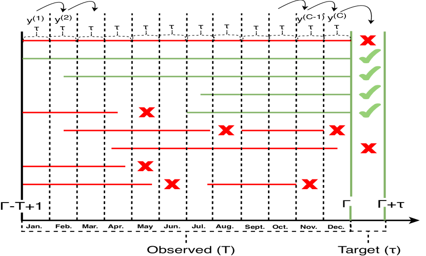
In this section, we focus on formulating the attrition prediction problem. To facilitate the problem formulation, we give a schematic illustration of user statuses as shown in Fig. 1. Suppose there are a set of N samples or users , for which we collect user data from the historical time period [-T+1, ] of length T, and we aim to predict their statuses in the future target time window [+1, +] of length 444Theoretically speaking, is flexible and can be any positive integer. In practice, it depends on business scenarios, which can be weekly, biweekly, monthly or longer periods..
The user data are composed of three primitive heterogeneous sub-components: activity logs on a basis of observed time granularity (e.g., day) , dynamic user information , and static user profiles , namely, . For the activity logs component, we denote any events happening during the time span T right prior to the target time window as .
The general goal is to search for a reasonable mapping rule from observed feature space to attrition statuses and subsequently apply to estimate the statuses of samples in the future. The probability of sample in attrition can be denoted as
| (1) |
Practically speaking, the ground truth is relatively subject to the future target time window [, ]. Specifically, if a user drops out of a course or is churned within this window, it is then labeled as ; if the user remains active, then it is labeled as 0. It is worth noting that attrition labels are generated based on the overall statuses of users during the target time window.
III-B Methodology
Section III-A introduces the primitive problem formulation. We propose to extend this formulation to incorporate multi-snapshot statuses according to the snapshot window, which is equal to the pre-designated target time window size . Concretely, sequential outputs are generated across sampled observed time period per units based on the attrition definition. We then can generate snapshot outputs. As for users with the observed time span being less than , we take zero-padding for the computational convenience. The corresponding masking indicators are introduced to disable their contributions to the loss as detailed in Eq. 8. Accordingly, we obtain the final series of statuses of sample as where is the status within the target time period. In this case, the conditional probability that sample is in the state of attrition can be represented as
| (2) |
Therefore, our learning rule can naturally evolve to be for target time step .
With the reformulation of this problem, we introduce different learning layers/components of BLA and discuss how these components tackle the aforementioned issues faced by the attrition prediction.
III-B1 Parallel Input Layer
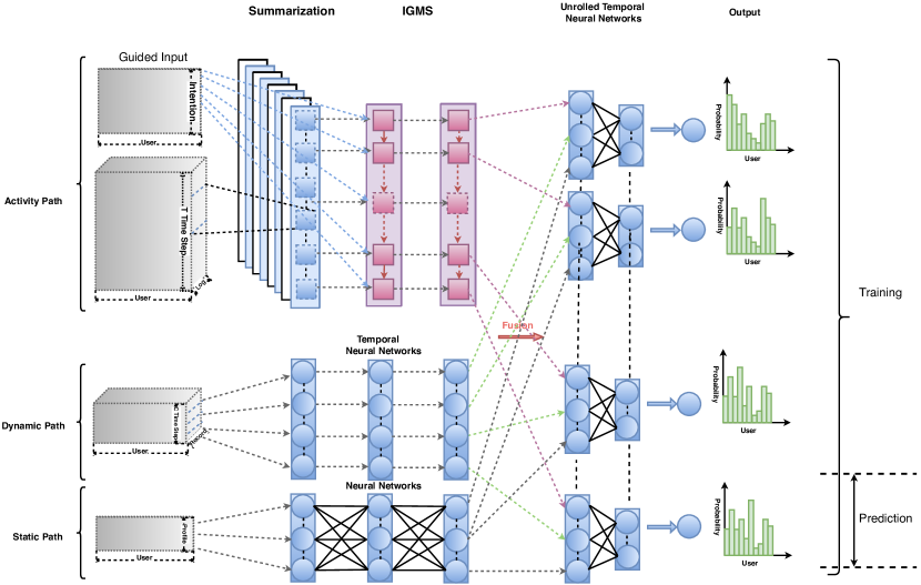
In accordance with reformulated mapping rule , the original feature space includes four different parts: activity logs, dynamic information, static profiles and precedent statuses. In this case, we design multiple parallel input layers for corresponding learning paths to solve the amalgamation problem associated with these heterogeneous multi-view features as diagrammed in Fig. 2.
Activity input layer– Three-dimensional users activity logs are fed into this layer, along which are user samples, observation time span, and activity metrics. Concretely, the granularity of primitive observation time can be, but not limited to, every minute, hourly, daily, weekly, monthly, or any reasonable time duration. The activities can be, but not limited to, students’ engagement for MOOCs, products booting, usage of specific features within the products for software companies. Dynamic input layer– Three-dimensional dynamic layer is responsible for the derivative of the user profile, products information or their interactive records based on the snapshot window. This includes, but not limited to, subscription age, payment settings (automatic renewal/cancellation), or any reasonable derivatives. Static input layer– This layer takes static profiles of users or products, which cover many details including but not limited to, gender, birthday, geographical location, market segments, registration/enrollment method or any other unchanging information. This layer is of the two-dimensional shape. Guided input layer– The snapshotted statuses as a two-dimensional guided intention is embodied into the attrition prediction through this layer.
III-B2 Summarization Layer
Closely following the activity input layer is the summarization layer, which is developed for summarizing user activities. Due to the homogeneity along the observed time and the heterogeneity across activity logs, we utilize one-dimensional CNN to aggregate low-level activity logs over a fine-grained time span (e.g., day) to generate high-level feature representation over a coarse-grained one (e.g., week). Mathematically speaking, we have
| (3) |
where is the input activity logs, and are the indices of output time step and activity summarizer, respectively. Summarizer is the weight matrix with and being the window size of summarizing time span and sequence channel, respectively. In particular, N of the first summarization layer is equal to the number of activity metrics. Activity logs can be summarized to be with different granularities via setting kernel size .
The designed summarization layer entails threefold benefits: (1) Learning rich relations and bypassing labor-intensive handcrafted efforts in summarizing primitive activity logs; (2) Upholding the interpretation track of primitive activity metrics compared with hand-operated aggregation; (3) Accelerating the training procedure of model thanks to the noise filtering and feature dimensionality reduction.
III-B3 Intention Guided LSTM Layer with Multiple Snapshot Outputs
In order to capture the long-range interactive dependency of summarized activities and make the most use of generated auxiliary statuses, we propose to introduce a variant of Long Short-Term Memory Networks (LSTM) [24]. To simplify the following notations, we omit sample indices here. The original formulation in the family of Recurrent Neural Networks [25, 26] (RNNs)555http://colah.github.io/posts/2015-08-Understanding-LSTMs/ is usually denoted as
| (4) |
where and are the input sequence of interest and the estimated hidden state vector or output at time , respectively. is the immediate precedent estimated state vector. We here propose to embed the actual immediate precedent status to guide the learning procedure as
| (5) |
As illustrated in Fig. 3, the core equations are accordingly updated as follows:
| (6) |
where denotes the element-wise Hadamard product. and are sigmoid and hyperbolic tangent activation functions, respectively. , , , are forget, input, output and cell states, which control the update dynamics of the cell and hidden outputs jointly. It is noted that multiple snapshot outputs in the training phase can keep track of the evolution of statuses sequentially and naturally. In the meantime, the introduced auxiliary statuses are complementary to activity, dynamic and static inputs in terms of capturing the intention progression. We call it IGMS as annotated in Fig. 2.
III-B4 Temporal Neural Network Layer
In order to guarantee the temporal order preservation of feature representation, we introduce temporal neural networks:
| (7) |
where is a temporal slice of the output of layer .
This layer entails twofold roles: (1) Feature learning over different snapshot periods in the dynamic path; (2) Fusion of feature representation in multiple paths. It is also noted that the activation function of the final temporal neural network layer is sigmoid.
III-B5 Decay Mechanism
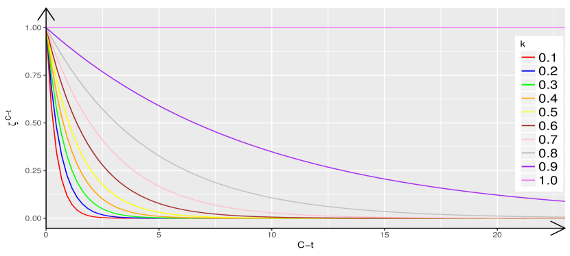
When multiple snapshot attrition statuses are incorporated into our learning framework, their associated impacts need to be adjusted in the training phase accordingly. This results from the fact that the underlying behavior patterns might change over time in a certain way [27]. To this end, we have a underlying assumption: the bigger the time gap between auxiliary snapshot statuses and attrition status at target time period is, the less similar the underlying intention patterns are. The temporal exponential decay is thus introduced to penalize weights based on this assumption. Concretely, , where depends on the expected speed of decay, as shown in Fig. 4. Since the decay speed is a hyper-parameter, it is determined by the validation dataset.
III-B6 Objective Function
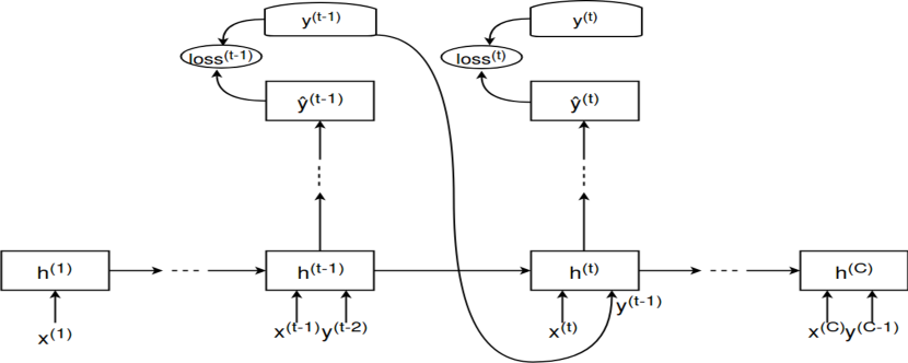
With auxiliary snapshot statuses being incorporated into the training phase as shown in Figs. 2 and 3, we have the following loss function to guide the learning procedure:
| (8) |
where and are temporal decay weight and sample-level binary masking indicator, respectively. In particular, can be used to mask invalid attrition statuses of training samples in the snapshot time periods caused by the calendar date alignment. For example, the registration dates of some users are later than the beginning of observed time periods as shown in Fig. 1.
As shown in Fig. 2. BLA mainly includes activity path, dynamic path and static path. In the activity path, the time granularity of input is on a basis of primitive observed time granularity (e.g., day), whereas output granularity is the snapshot window (e.g., month). The dynamic path is composed of temporal neural networks with both input and output being at the granularity of the snapshot span. For the static path, the outputs are forked times for further fusion with outputs of activity and static paths, as shown in unrolled temporal neural networks of Fig. 2.
III-B7 Predictive Inference
With the learning architecture and estimated parameters, we obtain the learned model ready for predicting user-intended actions. As illustrated in Fig. 2, we have only one output at the time period, which is the attrition probability of the target time period in prediction phase (validation and test).
III-C Feature Interpretation and Visualization
Saliency maps are one powerful technique to interpret and visualize feature representation behind deep neural networks, which have been widely utilized to analyze feature importance [22, 28]. In this paper, we also construct saliency maps by back-propagating features with the guidance of BLA to highlight how input features impact the user attrition. First of all, a user is supposed to have feature vector and the associated attrition state, we aim to figure out how elements of shape output probability of state . Regarding BLA, the score is a highly non-linear function of input . , however, can be approximated by a linear function in the closeness of based on the first-order Taylor expansion:
| (9) |
where is the first-order derivative of with respect to the feature vector at :
| (10) |
There are two points about the interpretation of this kind to consider: 1) The magnitude of the derivative indicates the extent to which the change of the most influential elements of feature vector on the probability of the attrition state; 2) The direction of each element of the derivative shows whether such a change boosts or decreases the probability of the attrition state. It is noted that the computation of the user-specific saliency map is very fast due to the requirement of a single back-propagation pass.
For dynamic and static inputs, we take average on saliency maps of all test users and then obtain the overall saliency map. The overall one can help to identify the underlying attrition and retention factors involved in the attrition directly. For activity logs with different metrics, we concentrate on exploring the evolution patterns of activity logs. Thus, we take the absolute value of saliency maps before averaging over all test users. Finally, we take sum of all metrics along observed time periods.
| # of user | # of attrition | # of persistence | observation span T (day) | snapshot window size (day) | target time period | |
|---|---|---|---|---|---|---|
| MOOCs | 120,542 | 95,581 | 24,961 | 30 | 10 | 10 days after the end of observed days |
| KKBox | 11,2118 | 19,415 | 92,703 | 720 | 30 | 02/01/2017 02/28/2017 |
| 156,029 | 21,752 | 134,277 | 720 | 30 | 03/01/2017 03/31/2017 |
IV Experiment
In this section, we first assess the performance of BLA on the customer attrition task comparing with competitive baselines for two public datasets and one private dataset. Then, we perform feature analysis to distill the evolving patterns of user activity logs, attrition and retention factors.
IV-A Experimental Setup
We utilize python libraries Keras666https://github.com/keras-team/keras to build the architecture of our learning algorithm and Tensorflow [29] to perform feature interpretation and visualization. NVIDIA Tesla K80 GPU with memory of 12GB is used for model development. Microsoft Azure with PySpark is adopted as the large-scale data processing platform.
Network Architecture. Along Activity Path are 1 one-dimensional CNN (14 kernels) and 2 intention-guided LSTM (30 and 15 kernels). Dynamic Path consists of 1 two-layered temporal neural networks with 30 and 15 hidden nodes. Static Path involves 1 two-layered neural networks with 30 and 15 hidden nodes. The fusion layer includes 1 two-layered temporal neural networks with 30 and 15 hidden nodes.
Training. We initialize parameters in BLA with Glorot uniform distribution [30]. The mini-batch size and the maximum number of epochs are set to be and , respectively. The parameters are updated based on Adam optimization algorithm [31] with learning rate of and decay factor of 1e-3. Early stopping of 20 epochs is set to prevent the overfitting. Trainable parameters and hyper-parameters are tuned based on the loss of attrition records in the validation dataset. As shown in Fig. 2, all historical records are incorporated into the loss function in formula (8).
Test. As shown in Fig. 2, the prediction is conducted on customer attrition records during the target time periods. With both the trained parameters and hyper-parameters, we measure the performance of the model on the specified target periods.
Training and test parts are split based on the temporal logic and will be detailed in the coming subsections accordingly.
IV-B Baseline Approaches
In this section, we will introduce alternative algorithms as baseline schemes to demonstrate the effectiveness of the proposed BLA. User activity logs are manually aggregated and then reshaped to be a vector. The one-month dynamic and static information are directly reshaped and then fused with logs vector to generate the learning features. The baselines are tuned based on the validation part and the optimal parameters are reported accordingly.
-
•
LR: The classical Logistic Regression [5] is commonly used with good interpretation capacity [9]. To facilitate the training with the large-scale dataset, we construct a simple neural network with one input layer and sigmoid activation function with GPU acceleration. Adam [31] with learning rate of 0.01 and decay rate of is adopted as the optimization algorithm for MOOCs and KKBox.
-
•
DNN: Generally speaking, stacking computational units can represent any probability distributions in a certain configured way [32]. Thus, vanilla deep neural networks are widely utilized for attrition prediction in the academic research [14, 15]. The network is with 2 hidden layers of 100, 10 nodes, respectively. Adam [31] with learning rate of 0.01 for MOOCs and 0.001 for KKBox, as well as decay rate of for both datasets is adopted.
- •
- •
-
•
SVM: SVM is explored in this regard as well [6, 7]. To scale better to large numbers of samples (the inherent problem in SVM training), we adopt liblinear (LinearSVC) for linear kernel, the bagging classifier (BaggingClassifier + SVC) for non-linear radial basis function (rbf) and polynomial (poly) kernels in Scikit-Learn library. The settings are linear kernel with for MOOCs and rbf kernel with for KKBox.
-
•
CNN: Convolutional neural networks [16] include two layers of one-dimensional convolutional neural networks with 14 and 7 kernels and the subsequent fully connected neural networks 30 and 15 hidden nodes.
-
•
LSTM: Vanilla recurrent neural networks or long short-term memory networks [17, 36] are also utilized here by aggregating activity logs with handcrafted efforts. One two-layered LSTM with 30-dimensional and 15-dimensional output nodes, followed by subsequent fully connected neural networks with 30 and 15 hidden nodes.
The variants of BLA are listed as follows: MSMP: a variant without intention guidance; IGMP: a variant without multi-snapshot mechanism; IGMS-AD: a variant only using activity path and dynamic path; IGMS-AS: a variant only using activity path and static path; IGMS-DS: a variant only using dynamic path and static path.
IV-C Evaluation Metrics
To measure the prediction performance of the proposed methodology, we adopt F1 Score, Matthews correlation coefficient (MCC) [37], the Area under Curves of Receiver Operating Characteristic (AUC@ROC) [38, 39, 40] and Curves of Precision-Recall (AUC@PR), respectively. As opposed to ROC curves, Precision-Recall curves are more sensitive to capture the subtle and informative evolution of algorithm’s performance. A more in-depth discussion is detailed in Ref. [41].
IV-D Experimental Results
We perform attrition prediction on two public attrition repositories MOOCs (dropout prediction)777https://biendata.com/competition/kddcup2015/ and KKBox (churn prediction)888https://www.kaggle.com/c/kkbox-churn-prediction-challenge based on BLA against baseline approaches. Furthermore, we apply the proposed method to users of Adobe Creative Cloud (CC) and compare it with random forest and the currently deployed model.
IV-D1 MOOCs and KKBox
Dropout in MOOCs and churn in subscription-based commercial products or services are two typical scenarios associated with the attrition problem. Dropout prediction focuses on the problem where we prioritize students who are likely to persist or drop out of a course, which is usually characterized by the highly skewed dominance of dropout over persistence. As opposed to dropout in MOOCs, churned users are in tiny proportion compared with persistent ones. The basic statistics of the MOOCs and KKBox datasets are described in Table I briefly. Here attrition labels indicate the user status within the target time period. As the given spans of the target time period are 10 days for MOOCs and one month for KKBox999 is pre-specified in datasets here., we set snapshot span as and accordingly. Given observation span and , a total of and outputs are generated simultaneously. The last one is the status to predict, and the precedent outputs are auxiliary statuses for aiding in the model development. User activity logs, dynamic and static features are given in Tables II and III, respectively. For MOOCs, the stratified data splitting is adopted since there are few overlapping time spans among different courses. Accordingly, the ratio of training, validation and testing datasets is 6:2:2. For KKBox, user records on Feb 2017 and March 2017 are utilized as model development and assessment, respectively. The development dataset is further split into internally stratified training and validation parts with ratio 8:2.
The comparison results among BLA and baselines are examined in Tables IV-D1 and IV-D1. Overall, BLA is able to outperform other commonly used methods for attrition prediction in terms of an array of metrics. In MOOCs, we report F1 score and AUC@PR based on minor persistent users, which is sensitive to the improvement of algorithms. It is noted that, as compared to baselines, the performance gain of BLA is more obvious in KKBox than that in MOOCs. There are two underlying causes: (1) Few dynamic and static user features are available for MOOCs, which degrades the power of the multi-path learning as shown in Table III; (2) The span of historical records is limited for MOOCs, which will suppress the multi-snapshot mechanism inevitably as shown in Table I.
| Dataset | Activity | Remarks |
| MOOCs | problem | working on course assignments |
| video | watching course videos | |
| access | accessing other course objects except videos and assignments | |
| wiki | accessing the course wiki | |
| discussion | accessing the course forum | |
| navigate | navigating to another part of the course | |
| page_close | closing the web page | |
| source | Event source (server or browser) | |
| category | the category of the course module | |
| KKBox | num_25 | # of songs played less than 25% of the song length |
| num_50 | # of songs played between 25% to 50% of the song length | |
| num_75 | # of songs played between 50% to 75% of the song length | |
| num_985 | # of songs played between 75% to 98.5% of the song length | |
| num_100 | # of songs played over 98.5% of the song length | |
| num_unq | # of unique songs played | |
| total_secs | total seconds played |
| Dataset | Style | Profile | Remarks |
| MOOCs | dynamic | — | — |
| static | course_id | course ID | |
| KKBox | dynamic | membership | the time to the initial registration |
| is_auto_renew | whether subscription plan is renewed automatically | ||
| is_cancel | whether subscription plan is canceled | ||
| static | bd | age when registered | |
| city | city when registration (21 anonymous categories) | ||
| gender | gender (male and female) | ||
| registered_via | registration method (5 anonymous categories) |
| Method | AUC@ROC | MCC | F1 Score | AUC@PR | |
|---|---|---|---|---|---|
| LR | 0.8595 | 0.5477 | 0.6017 | 0.7003 | |
| RF | 0.8693 | 0.5753 | 0.6430 | 0.7077 | |
| DNN | 0.8718 | 0.5786 | 0.6509 | 0.7157 | |
| NB | 0.8354 | 0.4976 | 0.5925 | 0.6562 | |
| SVM | 0.8656 | 0.5440 | 0.5924 | 0.7049 | |
| CNN | 0.8778 | 0.5851 | 0.6480 | 0.7324 | |
| LSTM | 0.8746 | 0.5863 | 0.6528 | 0.7246 | |
| \hdashline BLA | 0.8842 | 0.5973 | 0.6569 | 0.7464 | |
| Method | AUC@ROC | MCC | F1 Score | AUC@PR | |
|---|---|---|---|---|---|
| LR | 0.8292 | 0.6560 | 0.6986 | 0.7360 | |
| DNN | 0.9016 | 0.6005 | 0.6552 | 0.5937 | |
| RF | 0.9394 | 0.6961 | 0.7314 | 0.8085 | |
| NB | 0.5061 | 0.0314 | 0.2467 | 0.5671 | |
| SVM | 0.5960 | 0.2111 | 0.1091 | 0.4972 | |
| CNN | 0.8963 | 0.5409 | 0.5974 | 0.5263 | |
| LSTM | 0.9293 | 0.6786 | 0.7171 | 0.7779 | |
| \hdashline BLA | 0.9600 | 0.7280 | 0.7621 | 0.8436 | |
IV-D2 Ablation Analysis
To explore the potential explanation for BLA’s performance, a series of ablation experiments are conducted to study the role of key components of BLA. We focus on KKBox here due to the limited observation time span of MOOCs.
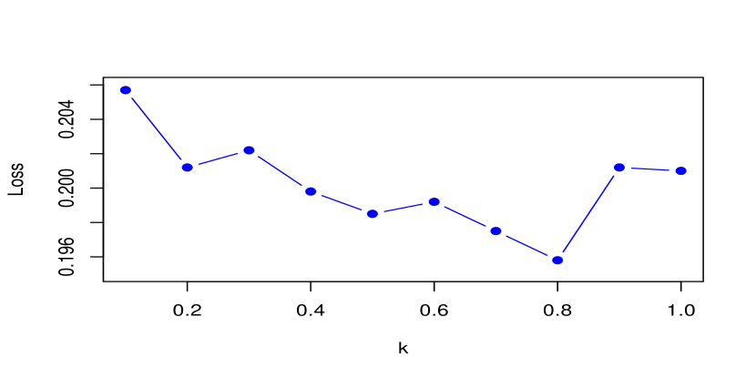
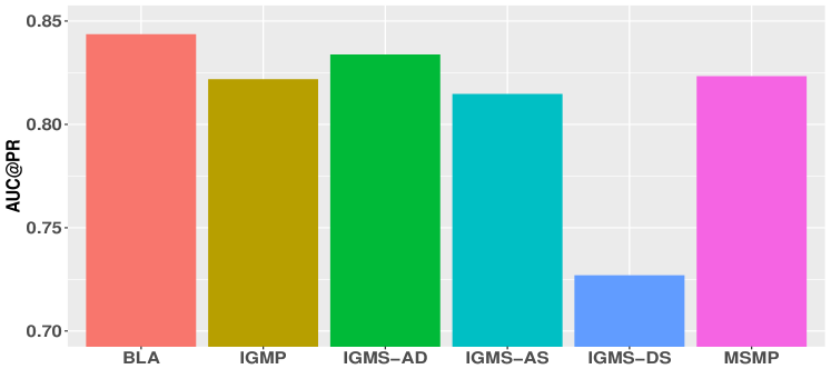
First of all, we empirically study the decay mechanism. As shown in Fig. 4, indicates all auxiliary statuses share equivalent weights in loss function, which also means that no decay mechanism is considered here. Meanwhile, when , it implies that auxiliary snapshot statuses are ignored and only the status of target time period is considered. The quasi U-shaped curve of loss on validation dataset demonstrates the existence of decay in attrition patterns over observed time steps as presented in Fig. 5. Furthermore, the evidence that the value of right side is less than that of left side suggests the necessity of the proposed multi-snapshot strategy. The performance of different variants of BLA is also reported in Fig. 6. Their performance disparity delivers useful points. To be specific, it is activity path that has the highest impact, followed by dynamic path and finally static path. Both intention guidance and multi-snapshot mechanisms shape BLA in different manners as well.
IV-D3 Attrition and Retention Factors
After attrition prediction, the next step typically is to identify underlying patterns/indicators or to explore feature importance.
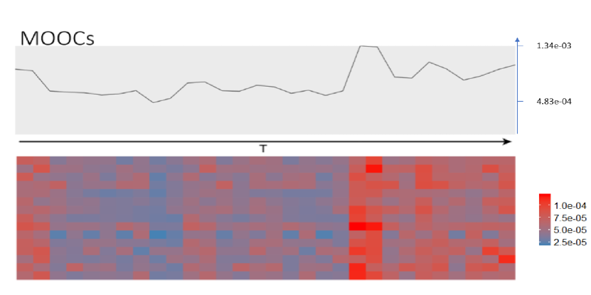
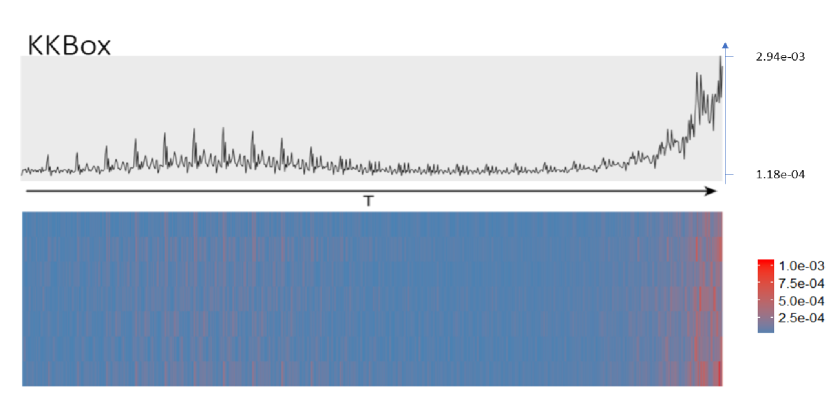
Regarding user activity logs, the feature importance across different observed time steps are visualized in Fig. 7. Overall, the feature importance changes periodically with the peak value in the vicinity of the intersection of two successive snapshots. Furthermore, the peak increases roughly as observation moves onwards to the target time period. The locality of peak values indicates user activities around payments are informative and important compared with other time steps. The evolution of peak values across different time periods shows that attrition within target time period is highly related to the proximate user activities, which is also intuitively reasonable.
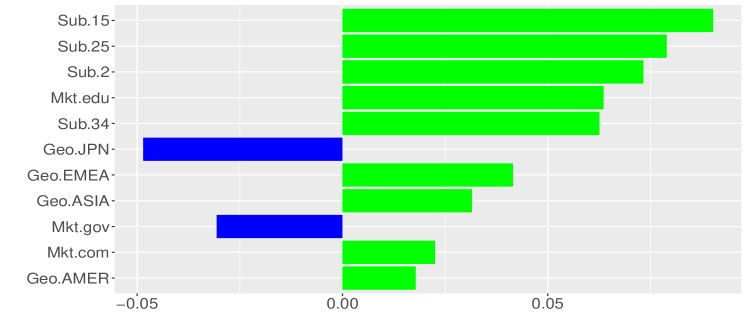
When it comes to dynamic and static user information, we also do in-depth analysis on KKBox. Among them, the most important features are is_cancel, and is_auto_renew from the dynamic side, and registered_via from the static side. As the registered method is provided anonymously, we cannot do any explanation. As shown in the top of Fig. 8, field is_cancel indicates whether a user actively cancels a subscription or not, which is proven to be positively correlated with attrition. It might be due to the change of service plans or other reasons, though. Naturally, feature is_auto_renew shows the intention of users to persist, which is also confirmed by the negative saliency value.

IV-D4 Adobe Creative Cloud
| sampling | T | target time period | ||
| yes | 1 | 360 | 30 | 05/01/2017 05/31/2017 |
| yes | 1 | 360 | 30 | 06/01/2017 06/30/2017 |
| no | — | 360 | 30 | 07/01/2017 07/31/2017 |
| Feature | Remarks | |
|---|---|---|
| Activity | Ps | booting times and total session time of Photoshop |
| Ai | booting times and total session time of Illustrator | |
| Id | booting times and total session time of InDesign | |
| Pr | booting times and total session time of PremierePro | |
| Lr | booting times and total session time of Lightroom | |
| Ae | booting times and total session time of AfterEffects | |
| En | booting times and total session time of MediaEncoder | |
| Dynamic | Sub | the subscription age of Adobe CC |
| Static | Mkt | market segment (education, government, and commercial) |
| Geo | general geographical code (JPN, EMEA, ASIA, AMER) |
Adobe CC provides entire collection of desktop and mobile applications for the brilliant design, which is characterized by low user attrition rate. We apply the preliminary version of BLA (without decay mechanism or guided intention) called pBLA101010Decay mechanism was not considered into our model during the internship period yet. to perform churn prediction and analysis on sampled users, which are briefed in Table VI. Concretely, user activity, dynamic and static information used in our model are described in Table VII. Regarding activity logs, two daily metrics booting times and total session time for each application (e.g., Photoshop) are recorded. Besides, we conduct both monthly and annual discretization of subscription age to capture two representative subscription types adopted by Adobe CC.
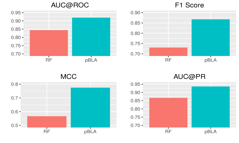
In our experiments, we consider users with subscription age of within 3 years. Due to confidentiality restrictions, we cannot disclose the volume of attrition and retention users. The dataset with the target time period of May 2017 is used for model development in which churned, and persistent users are sampled equivalently. We then evaluate the predictive capacity of our algorithm in two scenarios. In the first scenario, the test dataset includes sampled users with a ratio of 1:1 during target time period of June 1 to June 30, 2017. We then compare pBLA with widely used random forest in the industry (e.g., Framed Data) for attrition prediction [6, 8, 10]. The results are reported in Fig. 9. The significant performance gain can be gained here. In the other scenario, we compare our model with currently deployed model111111Features are created based on user profile and products usage logs. For the product usage feature, we mainly utilized user usage records of 7 top Adobe CC products to generate counts, rates, recency over different time windows for different types of events. We also performed extensive feature engineering, such as imputation, capping, logarithm, binning, interactions of two variables like ratios and products. Logistic regression based on multi-snapshot data was trained with elastic net regularization. Model hyper-parameters are tuned based on 5-fold cross-validation with the best of efforts. on users who were still active at the end of June 2017 (without sampling). Our proposed model beats the currently deployed model greatly as reported in Fig. 10121212The attrition probability adjustment of the currently deployed model is based on all users beyond the subscribed age of 3 years. We thus omit threshold based evaluation metrics.. The superiority of our algorithm over other approaches is more evident in Adobe CC than that in other datasets. This mainly results from the difference of the subscription plans. Most subscriptions of Adobe CC are the type of annual plan while other datasets experience a couple of months (e.g., 30 to 90 days for most KKBox subscriptions). The evolution of intended actions across long subscription plan period is amenable to our algorithm.
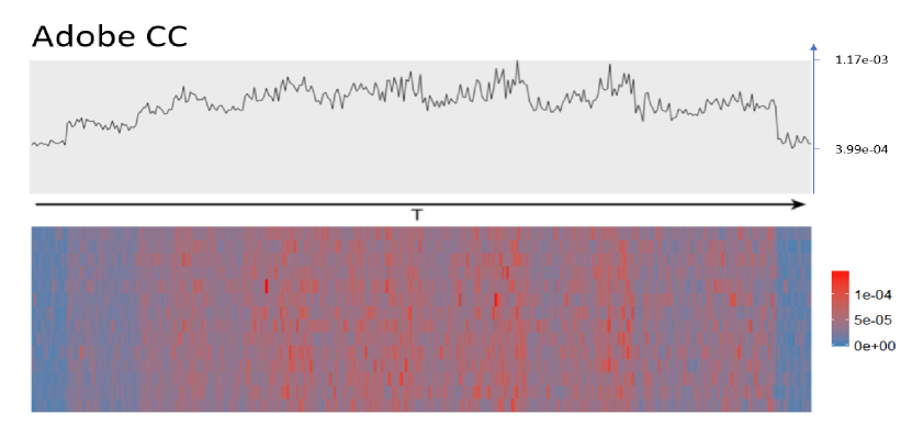
Likewise, the feature analysis implies that activity logs of users on applications of Adobe CC are characterized by the explicit periodicity in terms of impacts on attrition as shown in Fig. 11. Due to the long subscription plan for Adobe CC as mentioned before, the maximum of periodical peak values might be earlier than within the last month. Additionally, as shown in the bottom of Fig. 8, subscription age plays a very import role, for example, , , , month are the most risk months since the beginning of subscription, which are all around the renewal dates of annual subscription plan131313Monthly installment payment is available for the annual membership of Adobe CC.. Regarding static information, Japan (JPN) is found to be the most persistent area compared with other geographical areas. Also, it is easy to expect churn in subscribed users for the educational purpose, followed by the commercial and finally governmental purposes.

V Discussion and Future Work
The introduced user alignment based on the calendar timeline enables an unbiased modeling. The multi-path learning helps to fuse multi-view heterogeneous features, and the summarization layer is introduced to aggregate and integrate primitive user activity logs. In addition, we leverage IGMS with decay mechanism to track evolving intentions. Finally, saliency maps are introduced to elucidate the activity patterns, attrition and retention factors. There are some interesting aspects to explore in the future. First of all, from the perspective of the marketing campaign in the industry, the cost of attrition and retention may not be equivalent under some commercial circumstances. Thus, the probability threshold and corresponding loss function can be adaptively adjusted to account for their business profitability. In this case, some profit-driven strategies can be designed accordingly. Second, we consider the commonly used exponential decay in a trial-and-see way to explore the impacts of different time periods on the status of current time steps of interest. The hyper-parameter is determined by the validation dataset. It is desirable to develop a principled and feasible way to tune automatically and even discover the underlying decay evolution involved in the attrition prediction without the distribution assumption. This remains the topic of our future research.
VI Conclusion
In this work, we explore the classical attrition prediction (dropout and churn) problem and elucidate the underlying patterns. The proposed BLA is able to address an array of inherent difficulties involved in traditional attrition prediction algorithms. Particularly, the exploration of the decay mechanism further demonstrates the power and flexibility of our BLA in terms of capturing the evolving intended actions of users. The extensive experiments are conducted on two public real-world attrition datasets and Adobe Creative cloud user dataset. The corresponding results show that our model can deliver the best performance over alternative methods with high feasibility. The feature analysis pipeline also provides useful insights into attrition. Our work can also be applied to the attrition problem in related areas and other user intended actions.
Acknowledgment
We thank Sagar Patil for proofreading the manuscript.
References
- [1] S. Halawa, D. Greene, and J. Mitchell, “Dropout prediction in moocs using learner activity features,” Experiences and Best Practices in and around MOOCs, vol. 7, pp. 3–12, 2014.
- [2] W. Verbeke, K. Dejaeger, D. Martens, J. Hur, and B. Baesens, “New insights into churn prediction in the telecommunication sector: A profit driven data mining approach,” EJOR, vol. 218, no. 1, pp. 211–229, 2012.
- [3] R. B. Woodruff, “Customer value: the next source for competitive advantage,” JAMS, vol. 25, no. 2, pp. 139–153, 1997.
- [4] T. Vafeiadis, K. I. Diamantaras, G. Sarigiannidis, and K. C. Chatzisavvas, “A comparison of machine learning techniques for customer churn prediction,” Simul Model Pract Theory, vol. 55, pp. 1–9, 2015.
- [5] G. Nie, W. Rowe, L. Zhang, Y. Tian, and Y. Shi, “Credit card churn forecasting by logistic regression and decision tree,” Expert Syst Appl, vol. 38, no. 12, pp. 15 273–15 285, 2011.
- [6] K. Coussement and D. Van den Poel, “Churn prediction in subscription services: An application of support vector machines while comparing two parameter-selection techniques,” Expert Syst Appl, vol. 34, no. 1, pp. 313–327, 2008.
- [7] M. A. H. Farquad, V. Ravi, and S. B. Raju, “Churn prediction using comprehensible support vector machine: An analytical crm application,” Applied Soft Computing, vol. 19, pp. 31–40, 2014.
- [8] Y. Xie, X. Li, E. Ngai, and W. Ying, “Customer churn prediction using improved balanced random forests,” Expert Syst Appl, vol. 36, no. 3, pp. 5445–5449, 2009.
- [9] S. Nagrecha, J. Z. Dillon, and N. V. Chawla, “Mooc dropout prediction: lessons learned from making pipelines interpretable,” in WWW. IW3C2, 2017, pp. 351–359.
- [10] P. Spanoudes and T. Nguyen, “Deep learning in customer churn prediction: Unsupervised feature learning on abstract company independent feature vectors,” arXiv preprint arXiv:1703.03869, 2017.
- [11] A. Idris, A. Khan, and Y. S. Lee, “Genetic programming and adaboosting based churn prediction for telecom,” in SMC. IEEE, 2012, pp. 1328–1332.
- [12] W.-H. Au, K. C. Chan, and X. Yao, “A novel evolutionary data mining algorithm with applications to churn prediction,” TEVC, vol. 7, no. 6, pp. 532–545, 2003.
- [13] M. C. Mozer, R. Wolniewicz, D. B. Grimes, E. Johnson, and H. Kaushansky, “Predicting subscriber dissatisfaction and improving retention in the wireless telecommunications industry,” TNN, vol. 11, no. 3, pp. 690–696, 2000.
- [14] A. Sharma, D. Panigrahi, and P. Kumar, “A neural network based approach for predicting customer churn in cellular network services,” arXiv preprint arXiv:1309.3945, 2013.
- [15] C.-F. Tsai and Y.-H. Lu, “Customer churn prediction by hybrid neural networks,” Expert Syst Appl, vol. 36, no. 10, pp. 12 547–12 553, 2009.
- [16] A. Wangperawong, C. Brun, O. Laudy, and R. Pavasuthipaisit, “Churn analysis using deep convolutional neural networks and autoencoders,” arXiv preprint arXiv:1604.05377, 2016.
- [17] Z. Kasiran, Z. Ibrahim, and M. S. M. Ribuan, “Mobile phone customers churn prediction using elman and jordan recurrent neural network,” in Computing and Convergence Technology (ICCCT), 2012 7th International Conference on. IEEE, 2012, pp. 673–678.
- [18] C.-P. Wei and I.-T. Chiu, “Turning telecommunications call details to churn prediction: a data mining approach,” Expert Syst Appl, vol. 23, no. 2, pp. 103–112, 2002.
- [19] G. Song, D. Yang, L. Wu, T. Wang, and S. Tang, “A mixed process neural network and its application to churn prediction in mobile communications,” in ICDMW. IEEE, 2006, pp. 798–802.
- [20] J. Lu, “Predicting customer churn in the telecommunications industry—-an application of survival analysis modeling using sas,” SUGI, pp. 114–27, 2002.
- [21] M. T. Ribeiro, S. Singh, and C. Guestrin, “Model-agnostic interpretability of machine learning,” arXiv preprint arXiv:1606.05386, 2016.
- [22] K. Simonyan, A. Vedaldi, and A. Zisserman, “Deep inside convolutional networks: Visualising image classification models and saliency maps,” arXiv preprint arXiv:1312.6034, 2013.
- [23] M. T. Ribeiro, S. Singh, and C. Guestrin, “Why should i trust you?: Explaining the predictions of any classifier,” in SIGKDD. ACM, 2016, pp. 1135–1144.
- [24] S. Hochreiter and J. Schmidhuber, “Long short-term memory,” Neural Comput, vol. 9, no. 8, pp. 1735–1780, 1997.
- [25] D. E. Rumelhart, G. E. Hinton, and R. J. Williams, “Learning internal representations by error propagation,” California Univ San Diego La Jolla Inst for Cognitive Science, Tech. Rep., 1985.
- [26] I. Goodfellow, Y. Bengio, and A. Courville, Deep Learning. MIT Press, 2016, http://www.deeplearningbook.org.
- [27] F. Tan, C. Cheng, and Z. Wei, “Time-aware latent hierarchical model for predicting house prices,” in ICDM. IEEE, 2017, pp. 1111–1116.
- [28] F. Tan, X. Hou, J. Zhang, Z. Wei, and Z. Yan, “A deep learning approach to competing risks representation in peer-to-peer lending,” TNNLS.
- [29] M. Abadi, A. Agarwal, P. Barham, E. Brevdo, Z. Chen, C. Citro, G. S. Corrado, A. Davis, J. Dean, M. Devin et al., “Tensorflow: Large-scale machine learning on heterogeneous distributed systems,” arXiv preprint arXiv:1603.04467, 2016.
- [30] X. Glorot and Y. Bengio, “Understanding the difficulty of training deep feedforward neural networks,” in AISTATS, 2010, pp. 249–256.
- [31] D. P. Kingma and J. Ba, “Adam: A method for stochastic optimization,” arXiv preprint arXiv:1412.6980, 2014.
- [32] Y. Bengio et al., “Learning deep architectures for ai,” Foundations and Trends® in Machine Learning, vol. 2, no. 1, pp. 1–127, 2009.
- [33] S. V. Nath and R. S. Behara, “Customer churn analysis in the wireless industry: A data mining approach,” in Proceedings-annual Meeting of the Decision Sciences Institute, 2003, pp. 505–510.
- [34] B. Huang, M. T. Kechadi, and B. Buckley, “Customer churn prediction in telecommunications,” Expert Syst Appl, vol. 39, no. 1, pp. 1414–1425, 2012.
- [35] H. Zhang, “The optimality of naive bayes,” AAAI, vol. 1, no. 2, p. 3, 2004.
- [36] M. Fei and D.-Y. Yeung, “Temporal models for predicting student dropout in massive open online courses,” in ICDMW. IEEE, 2015, pp. 256–263.
- [37] B. W. Matthews, “Comparison of the predicted and observed secondary structure of t4 phage lysozyme,” Biochimica et Biophysica Acta (BBA)-Protein Structure, vol. 405, no. 2, pp. 442–451, 1975.
- [38] F. Tan, Y. Xia, and B. Zhu, “Link prediction in complex networks: a mutual information perspective,” PloS ONE, vol. 9, no. 9, p. e107056, 2014.
- [39] F. Tan, C. Cheng, and Z. Wei, “Modeling real estate for school district identification,” in ICDM. IEEE, 2016, pp. 1227–1232.
- [40] F. Tan, K. Du, Z. Wei, H. Liu, C. Qin, and R. Zhu, “Modeling item-specific effects for video click,” in SDM. SIAM, 2018, pp. 639–647.
- [41] J. Davis and M. Goadrich, “The relationship between precision-recall and roc curves,” in ICML. ACM, 2006, pp. 233–240.