Persistent -Cycles: Definition, Computation, and Its Application††thanks: Supported by NSF grants CCF-1740761 and CCF-1839252.
Abstract
Persistence diagrams, which summarize the birth and death of homological features extracted from data, are employed as stable signatures for applications in image analysis and other areas. Besides simply considering the multiset of intervals included in a persistence diagram, some applications need to find representative cycles for the intervals. In this paper, we address the problem of computing these representative cycles, termed as persistent -cycles, for -persistent homology with coefficients. The definition of persistent cycles is based on the interval module decomposition of persistence modules, which reveals the structure of persistent homology. After showing that the computation of the optimal persistent -cycles is NP-hard, we propose an alternative set of meaningful persistent -cycles that can be computed with an efficient polynomial time algorithm. We also inspect the stability issues of the optimal persistent -cycles and the persistent -cycles computed by our algorithm with the observation that the perturbations of both cannot be properly bounded. We design a software which applies our algorithm to various datasets. Experiments on 3D point clouds, mineral structures, and images show the effectiveness of our algorithm in practice.
1 Introduction
Persistent homology [18] is an important invention leading to Topological Data Analysis, where the associated persistence diagrams serve as stable signatures for various datasets [10] including the ones in image analysis [6, 14]. Persistent homology has its theoretical foundations rooted in quiver theory [11], in which case any persistence module indexed by a finite subcategory of can be decomposed into a direct sum of interval modules and the set of intervals of the interval modules, which constitute the persistence diagram, is unique for a persistence module [7].
Besides simply incorporating the persistence diagrams, some applications bring about the need of finding representative cycles for persistent homology [19, 26]. The computation of representative cycles for homology groups with coefficients has been extensively studied over the decades. While a polynomial time algorithm computing an optimal basis for first homology group [15] has been proposed, finding an optimal basis for dimension greater than one and localizing a homology class of any dimension are proved NP-hard [9]. There are a few works addressing the problem of finding representatives for persistent homology, some of which compute an optimal cycle at the birth index of an interval but do not consider what actually die at the death index [19, 20]. Obayashi [23] formalizes the computation of optimal representatives for a finite interval as an integer programming problem. He advocates solving it with linear programs though the correctness is not necessarily guaranteed. Wu et al. [26] proposed an algorithm for computing an optimal representative for a finite interval with a worst-case complexity exponential to the cardinality of the persistence diagram.
In this paper, we study the problem of computing representative cycles for persistent first homology group (-persistent homology) with coefficients. We term theses cycles as persistent -cycles and show that the computation of the optimal cycles is NP-hard. Then, we propose an alternative set of meaningful persistent -cycles with an efficient polynomial time algorithm. Specifically, as interval module decomposition reveals the structure of persistence modules, we define persistent cycles which fit into this structure directly. Although similar definitions for finite intervals have already been proposed [23, 26], to our knowledge, explicit explanation of how the representative cycles are related to persistent homology has not been addressed. Furthermore, we inspect the stability of the minimal persistent -cycles and persistent -cycles computed by our algorithm. The perturbations of both classes of cycles turn out to be unstable. So, in this regard, our polynomial time algorithm is not any worse than an optimal cycle generating algorithm though is much more efficient in terms of the time complexity.
We use a software based on our algorithm to generate tight persistent -cycles on 3D point clouds and 2D images as shown in Figure 1. We experiment with various datasets commonly used in geometric modeling, computer vision and material science, details of which are given in Section 6. The software, named PersLoop, along with an introductory video and other supplementary materials are available at the project website http://web.cse.ohio-state.edu/~dey.8/PersLoop.
2 Background
In this paper, we adopt the categorical definition of persistence module [4]. A category consists of objects and morphisms from an object to another object. A functor from to another category is a mapping such that any object of is mapped to an object of and any morphism of is mapped to a morphism of . We recommend [1] for the exact definitions of categories and functors. The definition of persistence module relies on some common categories: The category (the category alike) consists of objects from and a unique morphism from to if . We also denote the morphism from to as . The category consists of objects which are all the simplicial complexes and morphisms which are simplicial maps. The category consists of objects which are all the vector spaces over and morphisms which are linear maps. A persistence module is then defined as a functor *** Sometimes we also call a functor as a persistence module..
A persistence module is usually induced by a filtration of a simplicial complex , where the filtration is a filtered sequence of subcomplexes of such that and differ by one simplex . We can also interpret a filtration as a functor , where for , for , and a morphism is the inclusion. Denoting as the homology functor with coefficients, the -persistence module of is obtained by composing the two functors and , that is, . Specifically, for , for , and the morphism ††† when . is the linear map induced by the inclusion.
A special class of persistence modules is the interval modules. Given an interval , an interval module is defined as: for and otherwise; is the identity map for and is the zero map otherwise. By quiver theory, a -persistence module obtained from a finite complex has a unique decomposition in terms of interval modules, where is a finite index set [7]. Let denote the set of intervals of the interval modules which decomposes into. Observe that is also called the barcode or persistence diagram in the literature [17]. Sometimes we will abuse the notation slightly to write , where the argument is the filtration instead of the module it generates.
3 Persistent basis and cycles
Definition 1 (Persistent Basis).
An indexed set of -cycles is called a persistent -basis for a filtration if and for each and , .
Definition 2 (Persistent Cycle).
For an interval , a -cycle is called a persistent -cycle for the interval, if one of the following holds:
-
•
, is a cycle in containing , and is not a boundary in but becomes a boundary in ;
-
•
and is a cycle in containing .
Remark 1.
The following theorem characterizes each cycle in a persistent basis:
Theorem 1.
An indexed set of -cycles is a persistent -basis for a filtration if and only if and is a persistent -cycle for every interval .
Proof.
Suppose is an indexed set of -cycles satisfying the above conditions. For each , we construct an interval module , such that for and otherwise. We claim that . We first prove that for each , by proving that forms a basis of . Using mathematical induction, since is a vertex, this is trivially true. Suppose for this is true. If is neither positive nor negative, i.e., by the isomorphism induced from the inclusion, this is also trivially true for . If is positive, suppose the corresponding interval of is (note that and could possibly be ). Since are still independent in and is not in the span of them, then are independent in . Since the cardinality of equals the dimension of , it must form a basis of . If is negative, then there must be a for a such that . For any , , where . If , then , because in . Then spans . This means that it also forms a basis of . It is then obvious that the direct sums of the maps of the interval modules are actually the maps of , so is a persistent -basis for .
Suppose is a persistent -basis for . For each , must not be in , because otherwise would be in the image of . It is obvious that must contain . Note that for each and each , . Then for each such that , in and in . ∎
4 Minimal persistent -basis and their limitations
We have already defined persistent basis, the optimal versions of which are of particular interest because they capture more geometric information of the space. The cycles for an optimal (minimal) persistent basis have already been defined and studied in [20, 23]. In particular, the author of [23] proposed an integer program to compute these cycles. Although these integer programs can be solved exactly by linear programs for certain cases [13], the integer program is NP-hard in general. This of course does not settle the question of whether the problem of computing minimal persistent -cycles is NP-hard or not. We prove that it is indeed NP-hard and thus has no hope of admitting a polynomial time algorithm unless .
Consider a simplicial complex with each edge being assigned a non-negative weight. We refer to such as a weighted complex. For a -cycle in , define its weight to be the sum of all weights of its edges.
Definition 3 (Minimal Persistent -Cycle and -Basis).
Given a filtration on a weighted complex , a minimal persistent -cycle for an interval of is defined to be a persistent -cycle for the interval with the minimal weight. An indexed set of -cycles is a minimal persistent -basis for if for every , is a minimal persistent -cycle for .
We prove that the following special version of the problem of finding a minimal persistent -cycle is NP-hard. This special version reduces to the general version straightforwardly in polynomial time by assigning every edge a weight of .
Problem 1 (LST-PERS-CYC).
Given a filtration , and a finite interval , find a -cycle with the least number of edges which is born in and becomes a boundary in .
Theorem 2.
The problem LST-PERS-CYC is NP-hard
4.1 Instability of minimal persistent -cycles
In this section, we inspect the stability issues of the minimal persistent -cycles. Note that there may be multiple minimal persistent -cycles for an interval and an algorithm may choose anyone of them. This means that the cycles cannot be stable under those measures that take into account the entire geometry of the cycles (e.g., Hausdorff distance). In an attempt to sidestep this problem, we take a ‘weaker’ measure of the cycles which is still meaningful, namely their lengths. We show that even under such a measure, minimal persistent -cycles are unstable. Specifically, we consider the lower star filtration [17] of a vertex sequence, and inspect the perturbation of the lengths of persistent -cycles under the perturbation of the sequence. Since each interval in the -persistence diagram of a lower star filtration can be derived from an interval in the -persistence diagram of a corresponding insertion filtration‡‡‡ The insertion filtration is actually the filtration defined in Section 2., we can associate a persistent -cycle for to . The readers can verify that this assignment gives representatives for the decomposed interval modules of the -persistence module induced by the lower star filtration.
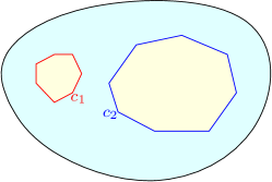
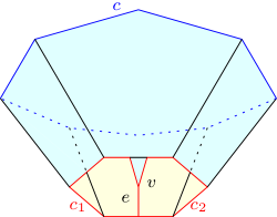
Figure 2a presents an example for which the perturbation of the minimal persistent -cycles cannot be properly bounded. The object in Figure 2a is a sphere with two holes (i.e., and ). We can assume that the object is nicely triangulated so that it becomes a simplicial complex. Let and be vertices from and . We can construct a filtration§§§ Note that we are constructing an insertion filtration for a lower star filtration. by first forming the two cycles and , with and being the last two vertices added, then adding the other parts of the simplicial complex. We then add a cone around to the filtration. We can first assume is added before , and the indices of and the apex vertex of the cone in the sequence are and . Then the minimal persistent -cycle for the interval is . If we switch and , the minimal cycle for the interval becomes . The difference of and can be made arbitrary under a single switch, which is the smallest possible perturbation of lower star filtration.
5 Computing meaningful persistent -cycles in polynomial time
Because the minimal persistent -cycles are not stable and their computation is NP-hard, we propose an alternative set of meaningful persistent -cycles which can be computed efficiently in polynomial time. We first present a general framework. Although the computed persistent -cycles have no guaranteed properties, the framework lays the foundation for the algorithm computing meaningful persistent -cycles that we propose later.
Algorithm 1.
Given a simplicial complex , a filtration , and , this algorithm finds a persistent -basis for . The algorithm maintains a basis for for every . Initially, let , then do the following for :
-
•
If is positive, find a -cycle containing in and let .
-
•
If is negative, find a set so that . This can be done in time by the annotation algorithm in [12]. Maintaining the annotations will take time altogether where has simplices and is the matrix multiplication exponent. Let be the greatest index in , then is an interval of . Assign to this interval as a persistent -cycle and let .
-
•
Otherwise, let .
At the end, for each cycle , assign as a persistent -cycle to the interval .
To prove the correctness of the algorithm, we need the following fact:
Proposition 1.
For a persistence module and a finite set of persistence modules , if and only if for each and for each .
Proof of Correctness of Algorithm 1.
Denoting all the intervals found by the algorithm as , we want to inductively prove that for all , the persistence module , which is the restriction of to , satisfies:
| (5.1) |
where the representative of is the persistent -cycle computed by the algorithm and the representative of is . When , is trivial and the equation is certainly true. Suppose for , the equation is satisfied. If is neither positive nor negative, or positive, then it is not hard to verify that the equation is still valid for by Proposition 1. If is negative, then we can let the persistent -cycle computed by the algorithm for be and be the greatest index in . Since is also created by , we can let the representative of the interval module for be . It is not hard then to verify that the equation is still satisfied for by Proposition 1. ∎
Based on Algorithm 1, we present another algorithm which produces meaningful persistent -cycles.
Algorithm 2.
In Algorithm 1, when is positive, let be the shortest cycle containing in . The cycle can be constructed by adding to the shortest path between vertices of in , which can be computed by Dijkstra’s algorithm applied to the -skeleton of .
Note that in Algorithm 2, a persistent -cycle for a finite interval is a sum of shortest cycles born at different indices. Since a shortest cycle is usually a good representative of its class, the sum of shortest cycles ought to be a good choice of representative for an interval. In some cases, when is negative, the sum contains only one component. The persistent -cycles computed by Algorithm 2 for such intervals are guaranteed to be optimal as shown below.
Proposition 2.
In Algorithm 2, when is negative, if , then is a minimal persistent -cycle for the interval ending with .
In Section 6 where we present the experimental results, we can see that, scenarios depicted by Proposition 2 occur quite frequently. Especially, for the larvae and nerve datasets, nearly all computed persistent -cycles contain only one component and hence are minimal.
A practical problem with Algorithm 2 is that unnecessary computational resource is spent for computing tiny intervals regarded as noise, especially when the user cares about significantly large intervals only. We present a more efficient algorithm for such cases.
Proof.
Note that must be unpaired before is added, this implies that . Since is the greatest index in , . ∎
Proposition 3 leads to Algorithm 3 in which we only compute the shortest cycles at the birth indices whose corresponding intervals contain the input interval . Since most of the time the user provided interval is a long interval, the intervals containing it constitute a small subset of all the intervals. This makes Algorithm 3 run much faster than Algorithm 2 in practice.
Input: The input of Algorithm 2 plus an interval
Output: A persistent -cycle for output by Algorithm 2.
Proposition 4 (Minimality Property).
Given that the minimal persistent -cycles are not stable, it is not surprising that the cycles computed by Algorithm 2 are also not stable under perturbation. Figure 2b presents an example for which the perturbation of persistent -cycles computed by Algorithm 2 cannot be properly bounded. We can construct a filtration by first forming the cycle then adding the other parts of the simplicial complex in Figure 2b, making the last vertex and the last simplex. We then add a cone around to the filtration. Let the indices of and the apex vertex of the cone in the vertex sequence be and . When is formed, the last edge of is positive, and is chosen as the shortest cycle containing . When is added, we can make and be the two shortest cycles containing . When is coned, if is chosen as the shortest cycle containing , then the persistent -cycle for the interval would be . Otherwise, the persistent -cycle would be . The length of can be arbitrary, so that the difference of the two persistent -cycles can be arbitrary under the same insertion filtration of the same lower star filtration.
6 Results and experiments
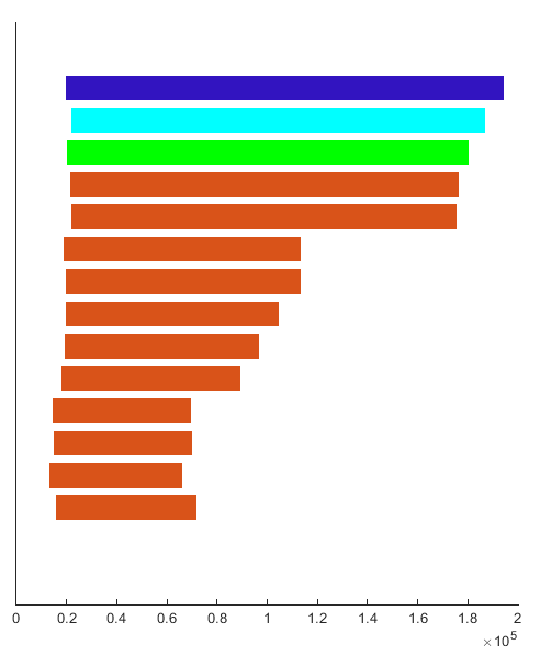
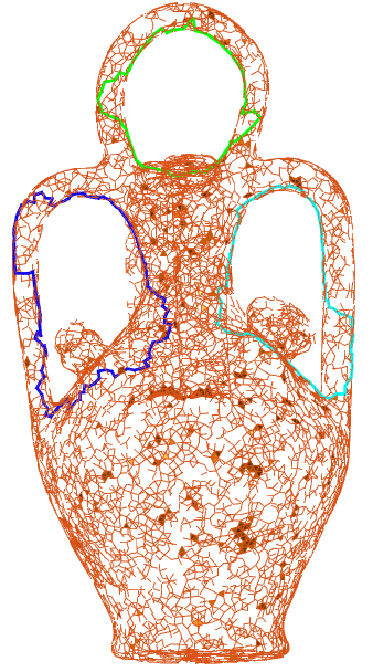
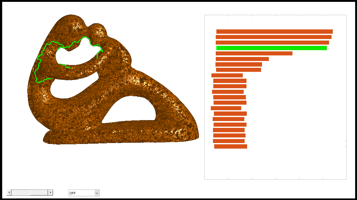
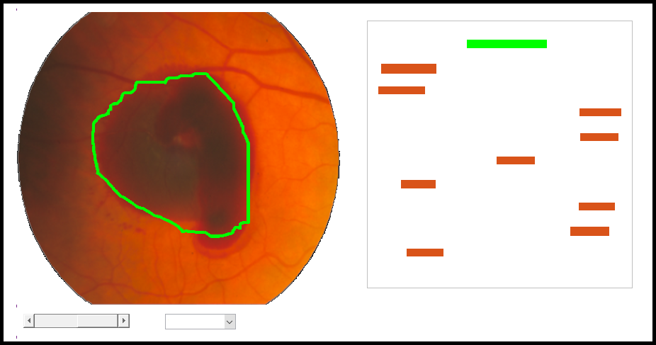
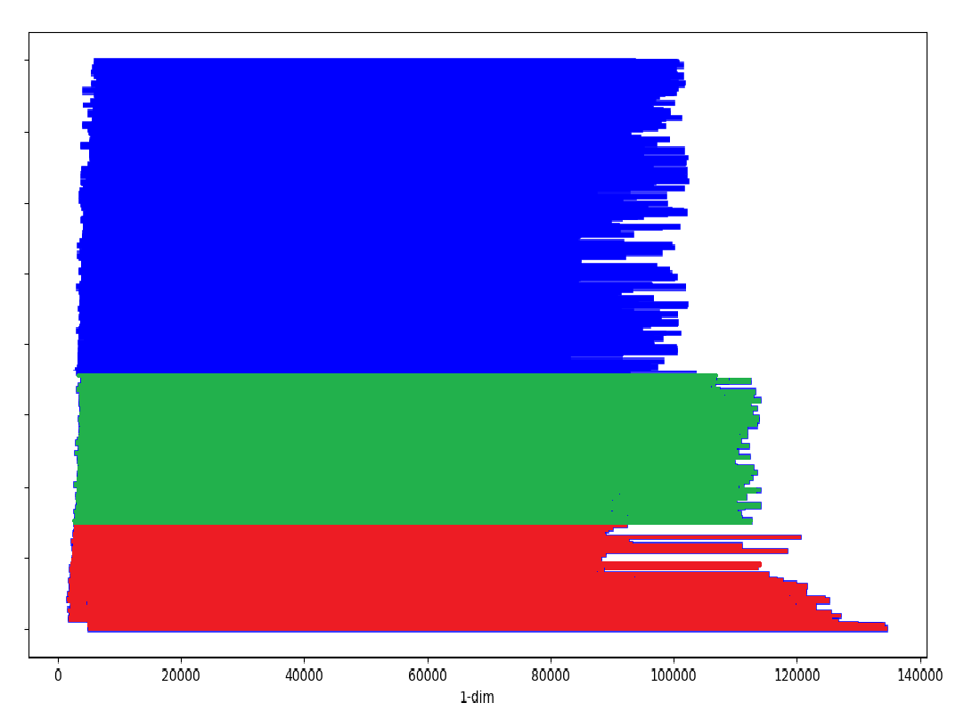
Our software PersLoop implements Algorithm 3. Given a raw input, which is a 2D image or a 3D point cloud, and a filtration built from the raw input, the software first generates and plots the barcode of the filtration. The user can then click an individual bar to obtain the persistent -cycle for the bar (Figure 3). The experiments on 3D point clouds and 2D images using the software show how our algorithm can find meaningful persistent -cycles in several geometric and vision related applications.
6.1 Persistent -cycles for 3D point clouds
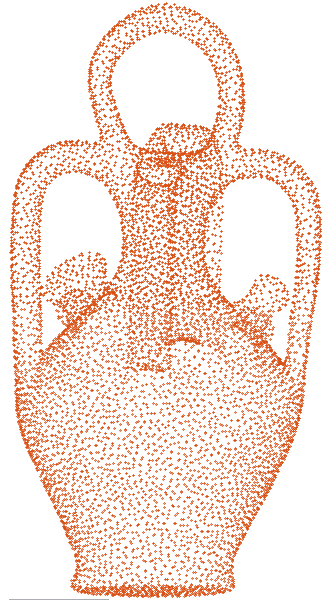
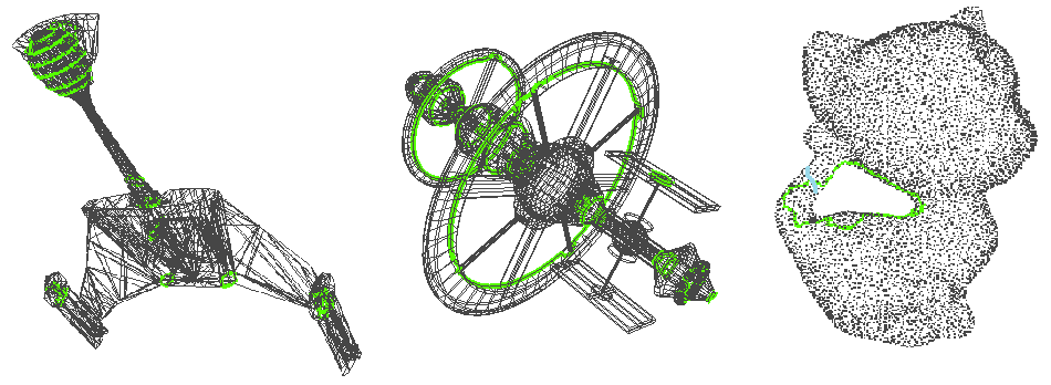
We take a 3D point cloud as input and build a Rips filtration using the Gudhi library [25]. As shown in Figure 4, persistent -cycles computed for the three point clouds sampled from various models are tight and capture essential geometrical features of the corresponding persistent homology. Note that our implementation of Algorithm 3 runs very fast in practice. For example, it took 0.3 secs to generate 50 cycles on a regular commodity laptop for the Botijo (Figure 1a) point cloud of size 10,000.
6.2 Image segmentation and characterization using cubical complex
In this section, we show the application of our algorithm on image segmentation and characterization problems. We interpret an image as a piecewise linear function on a 2-dimensional cubical complex. The cubical complex for an image has a vertex for each pixel, an edge connecting each pair of horizontally or vertically adjacent vertices, and squares to fill all the holes such that the complex becomes a disc. The function values on the vertices are the density or color values of the corresponding pixels. The lower star filtration [17] of the PL function is then built and fed into our software. We use the coning based annotation strategy [12] to compute the persistence diagrams. In our implementation, a cubical tree, which is similar to the simplicial tree [3], is built to store the elementary cubes. Each elementary cube points to a row in the annotation matrix via the union find data structure. The simplicial counterpart of this association technique is described in [2].
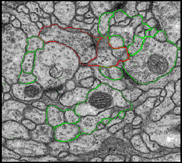
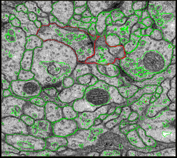
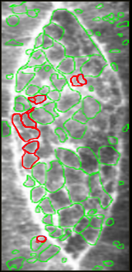
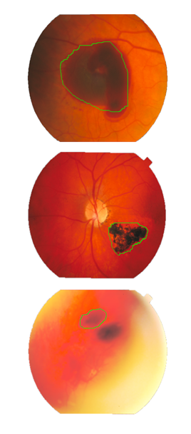
Our first experiment is the segmentation of a serial section Transmission Electron Microscopy (ssTEM) data set of the Drosophila first instar larva ventral nerve cord (VNC) [5]. The segmentation result is shown in Figures 5a and 5b, from which we can see that the cycles are in exact correspondence to the membranes hence segment the nerve regions quite appropriately. The difference between Figure 5a and 5b shows that longer intervals tend to have longer cycles. Another similar application is the segmentation of the low magnification micrographs of a Drosophila embryo [22]. As seen in Figure 5c, the cycles corresponding to the top 200 longest intervals indicate that the larvae image is properly segmented.
We experiment on another dataset from the STARE project [21] to show how persistent -cycles computed by our algorithm can be utilized for characterization of images. The dataset contains ophthalmologist annotated retinal images which are either healthy or suffering from diseases. Our aim is to automatically identify retinal and sub-retinal hemorrhages, which are black patches of blood accumulated inside eyes. Figures 1e and 3b show that a very tight cycle is derived around each dark hemorrhage blob even when the input is noisy.
6.3 Hexagonal structure of crystalline solids
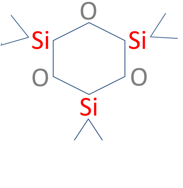
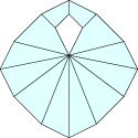
In this experiment, we use our persistent -cycles to describe the crystalline structure of silicate glass () commonly known as quartz. Silicate glass has a non-compact structure with three silicon and oxygen atoms arranged alternately in a hexagon as shown in Figure 6a. We build a weighted point cloud with the silicon and oxygen atoms arranged according to the space group on the crystal structure as illustrated in Figure 6b. The weights of the points correspond to the atomic weights of the atoms. On this weighted point cloud, we generate a filtration of weighted alpha complexes [16] by increasing from to .
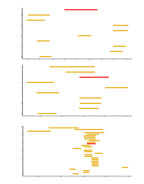
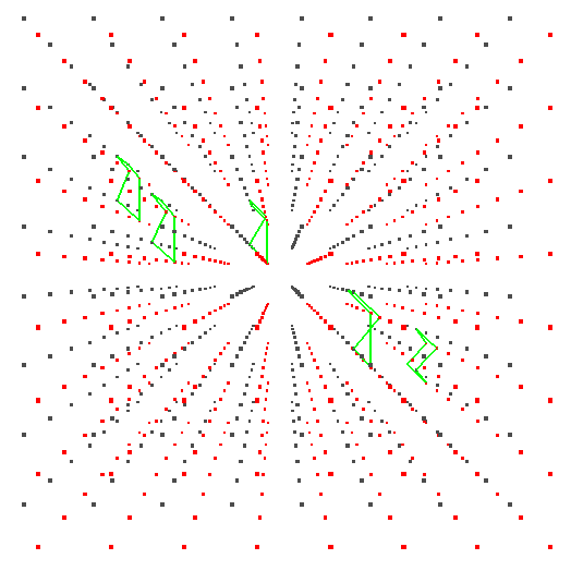
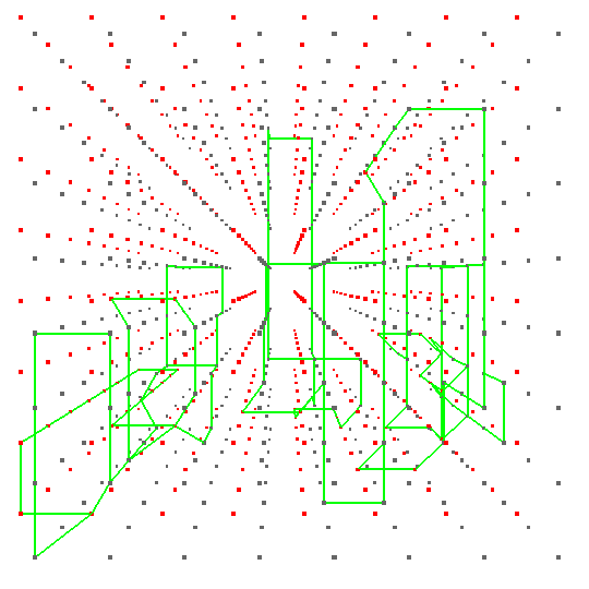
Persistent 1-cycles computed by our algorithm for this dataset reveal both the local and global structures of silicate glass. Figure 6d lists the barcode of the filtration we build and Figure 6b shows the persistent 1-cycles corresponding to the medium sized green bars in Figure 6d. We can see on close observation that the cycles in Figure 6b are in exact accordance to the hexagonal cyclic structure of quartz shown in Figure 6a. The larger persistent 1-cycles in Figure 6c, which span the larger lattice structure formed by our weighted point cloud, correspond to the longer red bars in Figure 6d. These cycles arise from the long-range order¶¶¶Long-range order is the translational periodicity where the self-repeating structure extends infinitely in all directions of the crystalline solid. This is evident from our experiment because if we increase the size of the input point cloud, these cycles grow larger to span the entire lattice.
References
- [1] Steve Awodey. Category theory. Oxford University Press, 2010.
- [2] Jean-Daniel Boissonnat, Tamal K. Dey, and Clément Maria. The compressed annotation matrix: an efficient data structure for computing persistent cohomology. CoRR, abs/1304.6813, 2013.
- [3] Jean-Daniel Boissonnat and Clément Maria. The simplex tree: An efficient data structure for general simplicial complexes. 20th Annual European Symposium, Ljubljana,Slovenia, (2):731–742, 2012.
- [4] Peter Bubenik and Jonathan A Scott. Categorification of persistent homology. Discrete & Computational Geometry, 51(3):600–627, 2014.
- [5] Saalfeld S Cardona A, Preibisch S, Schmid B, Cheng A, and Pulokas J et al. An integrated micro- and macroarchitectural analysis of the drosophila brain by computer-assisted serial section electron microscopy. PLoS Biol, 8, 2010.
- [6] Gunnar Carlsson, Tigran Ishkhanov, Vin Silva, and Afra Zomorodian. On the local behavior of spaces of natural images. Int. J. Comput. Vision, 76(1):1–12, January 2008.
- [7] Frédéric Chazal, Vin De Silva, Marc Glisse, and Steve Oudot. The structure and stability of persistence modules. Springer, 2016.
- [8] Chao Chen and Daniel Freedman. Quantifying homology classes ii: Localization and stability. arXiv preprint arXiv:0709.2512, 2007.
- [9] Chao Chen and Daniel Freedman. Hardness results for homology localization. Discrete & Computational Geometry, 45(3):425–448, 2011.
- [10] David Cohen-Steiner, Herbert Edelsbrunner, and John Harer. Stability of persistence diagrams. In Proceedings of the twenty-first annual symposium on Computational geometry, pages 263–271. ACM, 2005.
- [11] Harm Derksen and Jerzy Weyman. Quiver representations. Notices of the AMS, 52(2):200–206, 2005.
- [12] Tamal K. Dey, Fengtao Fan, and Yusu Wang. Computing topological persistence for simplicial maps. In Proceedings of the thirtieth annual symposium on Computational geometry, page 345. ACM, 2014.
- [13] Tamal K. Dey, Anil Hirani, and Bala Krishnamoorthy. Optimal homologous cycles, total unimodularity, and linear programming. SIAM Journal on Computing, 40(4):1026–1044, 2011.
- [14] Tamal K. Dey, Sayan Mandal, and William Varcho. Improved Image Classification using Topological Persistence. In Matthias Hullin, Reinhard Klein, Thomas Schultz, and Angela Yao, editors, Vision, Modeling & Visualization. The Eurographics Association, 2017.
- [15] Tamal K. Dey, Jian Sun, and Yusu Wang. Approximating loops in a shortest homology basis from point data. In Proceedings of the twenty-sixth annual symposium on Computational geometry, pages 166–175. ACM, 2010.
- [16] Herbert Edelsbrunner. Weighted alpha shapes. Technical report, Champaign, IL, USA, 1992.
- [17] Herbert Edelsbrunner and John Harer. Computational topology: an introduction. American Mathematical Soc., 2010.
- [18] Herbert Edelsbrunner, David Letscher, and Afra Zomorodian. Topological persistence and simplification. In Foundations of Computer Science, 2000. Proceedings. 41st Annual Symposium on, pages 454–463. IEEE, 2000.
- [19] Kevin Emmett, Benjamin Schweinhart, and Raul Rabadan. Multiscale topology of chromatin folding. In Proceedings of the 9th EAI international conference on bio-inspired information and communications technologies (formerly BIONETICS), pages 177–180. ICST (Institute for Computer Sciences, Social-Informatics and Telecommunications Engineering), 2016.
- [20] Emerson G Escolar and Yasuaki Hiraoka. Optimal cycles for persistent homology via linear programming. In Optimization in the Real World, pages 79–96. Springer, 2016.
- [21] A. Hoover and M. Goldbaum. Locating the optic nerve in a retinal image using the fuzzy convergence of the blood vessels. IEEE Transactions on Medical Imaging, 22(8):951–958, Aug 2003.
- [22] Daniel P. Kiehart, Catherine G. Galbraith, Kevin A. Edwards, Wayne L. Rickoll, and Ruth A. Montague. Multiple forces contribute to cell sheet morphogenesis for dorsal closure in drosophila. The Journal of Cell Biology, 149(2):471–490, 2000.
- [23] Ippei Obayashi. Volume optimal cycle: Tightest representative cycle of a generator on persistent homology. arXiv preprint arXiv:1712.05103, 2017.
- [24] Christos H Papadimitriou and Mihalis Yannakakis. Optimization, approximation, and complexity classes. Journal of computer and system sciences, 43(3):425–440, 1991.
- [25] The GUDHI Project. GUDHI User and Reference Manual. GUDHI Editorial Board, 2015.
- [26] Pengxiang Wu, Chao Chen, Yusu Wang, Shaoting Zhang, Changhe Yuan, Zhen Qian, Dimitris Metaxas, and Leon Axel. Optimal topological cycles and their application in cardiac trabeculae restoration. In International Conference on Information Processing in Medical Imaging, pages 80–92. Springer, 2017.
Appendix A Proof of Theorem 2
Similar to [8], we will reduce the NP-hard MAX-2SAT [24] problem to LST-PERS-CYC. The MAX-2SAT is defined as:
Problem 2 (MAX-2SAT).
Given variables and clauses , with the clauses being the disjunction of at most two variables. Find an assignment of Boolean values to all the variables such that the maximal number of clauses are satisfied.
Proof of Theorem 2.
We will reduce MAX-2SAT to LST-PERS-CYC. Given an instance of MAX-2SAT, we first construct a simplicial complex as in [8], by forming a triangulated cylinder for each variable and a cycle for each clause , such that the two ends and of correspond to and and are the only two cycles with the least number of edges of their homology class in . To make the process clearer, our construction of the cycles , , and are a little different from [8]. Each or has edges and of them are bijectively assigned to the clauses, such that in between each two consecutive edges assigned to some clauses, there are two edges which are not assigned to any clause. For a clause cycle (do the similar for other cases), we assign three edges to and pick one edge to be shared with the edges in and assigned to . Let , then our construction will make it true that, there is an assignment of Boolean values making clauses satisfied if and only if there is a cycle in with edges.
Next we are going to construct a filtration of a complex , where . We first construct a filtration of , with the only restriction: Pick an edge of a clause cycle, which is not shared with any end cycle of the variable cylinders, and take as the last simplex added to the filtration. To construct and , we need to find all simple cycles of . A simple cycle is defined as a cycle such that, each vertex has degree and there is only one connected component in the cycle. We can use a DFS-based algorithm to find all simple cycles for : Treat as graph and run DFS on the graph. Find a non-DFS-tree edge of , then find the lowest common ancestor of and in the DFS tree. The paths in the DFS tree from to and to , plus the edge , form a simple cycle of . Delete the simple cycle from the graph and repeat the above process until the graph becomes empty.
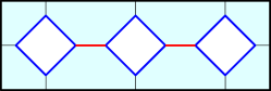
For each simple cycle of , we attach a cylinder to such that, one end of is , the other end of is a quadrilateral, and all the other edges of connect to the quadrilateral. An example of such a cylinder connecting a dodecagon and a quadrilateral is illustrated in Figure 7a. After all the cylinders are attached to the simple cycles, we get a simplicial complex . We can append the simplices of to , to get a filtration of . Since deformation retracts onto , all negative triangles of are paired with an edge of . We then construct a simplicial complex whose boundary is the sum of all the quadrilaterals and an outer cycle , as in Figure 7b, and attach this simplicial complex to by gluing the quadrilaterals, to get a simplicial complex . To form a filtration of , we first append the red edges in Figure 7b to , then append all the other simplices of . Finally, we form a cone around to get and append the missing simplices to get the filtration .
Let be the last triangle in , then it is true that deformation retracts to the union of and the red edges. This indicates that all negative triangles of , other than , are paired with edges of . Let the index of in be and the index of in be , we claim that is an interval of . To prove this, first note that is born in and becomes a boundary in . By the time is added, is unpaired. So by Algorithm 1, must be paired with .
Now we have constructed an instance of LST-PERS-CYC, from an instance of MAX-2SAT: Given the filtration and the interval , find a persistent -cycle with the least number of edges. We then prove that the answer to LST-PERS-CYC is also the answer to MAX-2SAT. First note that the map is injective. This means that any persistent -cycle for must be homologous to in , as they are homologous in . It follows that computing the minimal persistent -cycle of is equivalent to computing the minimal cycle of the homology class in , which is in turn equivalent to computing the answer for the original MAX-2SAT problem. Then we have had a reduction from MAX-2SAT to LST-PERS-CYC. Furthermore, the reduction is in polynomial time and the size of the constructed instance of LST-PERS-CYC is a polynomial function of that of MAX-2SAT, so LST-PERS-CYC is NP-hard. ∎