Downwinding for Preserving Strong Stability in Explicit Integrating Factor Runge–Kutta Methods

Abstract

Strong stability preserving (SSP) Runge–Kutta methods are desirable when evolving in time problems that have discontinuities or sharp gradients and require nonlinear non-inner-product stability properties to be satisfied. Unlike the case for $L_{2}$ linear stability, implicit methods do not significantly alleviate the time-step restriction when the SSP property is needed. For this reason, when handling problems with a linear component that is stiff and a nonlinear component that is not, SSP integrating factor Runge–Kutta methods may offer an attractive alternative to traditional time-stepping methods. The strong stability properties of integrating factor Runge–Kutta methods where the transformed problem is evolved with an explicit SSP Runge–Kutta method with non-decreasing abscissas was recently established. However, these methods typically have smaller SSP coefficients (and therefore a smaller allowable time-step) than the optimal SSP Runge–Kutta methods, which often have some decreasing abscissas. In this work, we consider the use of downwinded spatial operators to preserve the strong stability properties of integrating factor Runge–Kutta methods where the Runge–Kutta method has some decreasing abscissas. We present the SSP theory for this approach and present numerical evidence to show that such an approach is feasible and performs as expected. However, we also show that in some cases the integrating factor approach with explicit SSP Runge–Kutta methods with non-decreasing abscissas performs nearly as well, if not better, than with explicit SSP Runge–Kutta methods with downwinding. In conclusion, while the downwinding approach can be rigorously shown to guarantee the SSP property for a larger time-step, in practice using the integrating factor approach by including downwinding as needed with optimal explicit SSP Runge–Kutta methods does not necessarily provide significant benefit over using explicit SSP Runge–Kutta methods with non-decreasing abscissas.

This paper is in honor of Prof. Chi-Wang Shu’s sixtieth birthday.
His pioneering work on SSP methods and his observations on downwinding inspired this paper. We wish him many many more productive, happy, and healthy years to inspire many mathematicians.

1 Introduction

When numerically solving a hyperbolic conservation law of the form

$$U_{t}+f(U)_{x}=0,$$ (1)

specially designed spatial discretizations are used to handle the discontinuities in the solution that sometimes arise. These spatial discretizations typically satisfy some nonlinear non-inner-product strong stability properties when coupled with forward Euler time-stepping [3]. However, in practice we wish to use higher order time discretizations, which preserve the strong stability properties of the spatial discretization coupled with forward Euler.

Explicit strong stability preserving (SSP) Runge–Kutta methods were first developed in [13, 14] to evolve the semi-discretization

$$u_{t}=F(u),$$ (2)

resulting from approximating $f(u)_{x}$ with a total variation diminishing (TVD) spatial discretization. TVD spatial discretizations are specially designed to ensure that the forward Euler time-step is strongly stable

$$\|u^{n+1}\|=\|u^{n}+\Delta tF(u^{n})\|\leq\|u^{n}\|$$ (3)

under some step size restriction

$$0\leq\Delta t\leq\Delta t_{\textup{FE}}.$$ (4)

We wish to guarantee that the same type of strong stability property

$$\|u^{n+1}\|\leq\|u^{n}\|$$ (5)

is still satisfied when the TVD spatial discretization is coupled with a higher order time-stepping method. To do this, we use the fact that many higher order time discretization can be written as a convex combination of forward Euler steps.

It is simple to show that if we can re-write a higher order time discretization as a convex combination of forward Euler steps, then we can ensure that any convex functional property (5) that is satisfied by the forward Euler method will still be satisfied by the higher order time discretization, perhaps under a different time-step. For example, an $s$-stage explicit Runge–Kutta method can be written as:

$$u^{(0)} = u^{n},$$

$$u^{(i)} = \sum_{j=0}^{i-1}\left(\alpha_{i,j}u^{(j)}+\Delta t\beta_{i,j}F(u^{(j)})\right),\;\;\;\;i=1,...,s$$ (6)

$$u^{n+1} = u^{(s)}.$$

Each stage can be written as

$$u^{(i)}=\sum_{j=0}^{i-1}\alpha_{i,j}\left(u^{(j)}+\Delta t\frac{\beta_{i,j}}{\alpha_{i,j}}F(u^{(j)})\right)$$

provided that a given $\alpha_{i,j}$ is zero only if its corresponding $\beta_{i,j}$ is zero. Recall that for consistency, we must have $\sum_{j=0}^{i-1}\alpha_{i,j}=1$, so that as long as the coefficients $\alpha_{i,j}$ and $\beta_{i,j}$ are all non-negative, each stage can be rearranged into a convex combination of forward Euler steps. Thus we have

$$\|u^{(i)}\|=\left\|\sum_{j=0}^{i-1}\left(\alpha_{i,j}u^{(j)}+\Delta t\beta_{i,j}F(u^{(j)})\right)\right\|\leq\sum_{j=0}^{i-1}\alpha_{i,j}\,\left\|u^{(j)}+\Delta t\frac{\beta_{i,j}}{\alpha_{i,j}}F(u^{(j})\right\|\leq\|u^{n}\|,$$

(where the final inequality follows from (3) and (4)), for any time-step that satisfies

$$\Delta t\leq\min_{i,j}\frac{\alpha_{i,j}}{\beta_{i,j}}\Delta t_{\textup{FE}}.$$ (7)

If any of the $\beta$’s are equal to zero, we consider the corresponding ratio to be infinite.

In the case where a particular $\beta_{i,j}<0$, the SSP property can still be guaranteed provided that we modify the spatial discretization for these instances [14]. When $\beta_{i,j}$ is negative, $\beta_{i,j}F(u^{(k)})$ is replaced by $\beta_{i,j}\tilde{F}(u^{(k)})$, where $\tilde{F}$ approximates the same spatial derivative(s) as $F$, but the strong stability property $\|u^{n+1}\|\leq\|u^{n}\|$ holds for the first order Euler scheme, solved backward in time, i.e.,

$$u^{n+1}=u^{n}-\Delta t\tilde{F}(u^{n})$$ (8)

This can be achieved, for hyperbolic conservation laws, by solving the negative in time version of (1),

$$U_{t}-f(U)_{x}=0.$$

Numerically, the only difference is the change of the upwind direction. Thus, if $\alpha_{i,j}\geq 0$, all the intermediate stages $u^{(i)}$ in (1) are convex combinations of backward in time Euler and forward Euler operators, with $\Delta t$ replaced by $\frac{|\beta_{i,j}|}{\alpha_{i,j}}\Delta t$. Following the same reasoning as above, any strong stability bound satisfied by the backward in time and forward in time Euler methods will then be preserved by the Runge–Kutta method (1) where $F$ is replaced by $\tilde{F}$ whenever the corresponding $\beta$ is negative.

Clearly then, if we can re-write an explicit Runge–Kutta method as a convex combination of forward Euler steps (or, in the downwinded case, of forward Euler and backward in time Euler steps), the monotonicity condition (3) will be preserved by the higher-order time discretizations, under a modified time-step restriction $\Delta t\leq\mathcal{C}\Delta t_{\textup{FE}}$ where $\mathcal{C}=\min_{i,j}\frac{\alpha_{i,j}}{|\beta_{i,j}|}$. As long as $\mathcal{C}>0$, the method is called strong stability preserving (SSP) with SSP coefficient   $\mathcal{C}$ [13]. Methods that use the downwinded operator $\tilde{F}$ as well as the operator $F$ are called downwinded methods [3].

In the original papers, the term $\|\cdot\|$ in Equation (3) above represented the total variation semi-norm, and these methods were known as TVD time-stepping methods [13, 14]. However, the strong stability preservation property holds for any semi-norm, norm, or convex functional, as determined by the design of the spatial discretization, provided only that the forward Euler condition (3) holds, and that the time-discretization can be decomposed into a convex combination of forward Euler and backward in time Euler steps with $\mathcal{C}>0$.

The convex combination condition is not only a sufficient condition for strong stability preservation, it is also necessary for strong stability preservation [3, 10, 15]. This means that if a method cannot be decomposed into a convex combination of forward Euler steps, then we can always find some ODE with some initial condition such that the forward Euler condition is satisfied but the method does not satisfy the strong stability condition for any positive time-step [3].

Not every method can be decomposed into convex combinations of forward Euler steps with $\mathcal{C}>0$. For this reason, explicit SSP Runge–Kutta methods cannot exist for order $p>4$ [10, 12]. Furthermore, the SSP requirement is quite restrictive, so that all explicit $s$-stage Runge–Kutta methods have an SSP bound $\mathcal{C}\leq s$ [3]. Moreover, this upper bound cannot usually be attained. Nevertheless, many efficient explicit SSP Runge–Kutta methods exist and are discussed in Section 3. Implicit SSP Runge–Kutta methods have been an active area of investigation as well; these methods have an order barrier of $p\leq 6$, and seem to exhibit an SSP bound $\mathcal{C}\leq 2s$ [3]. This disappointing result limits the interest in implicit SSP Runge–Kutta methods, as well as in implicit-explicit SSP Runge–Kutta methods, studied in [1].

Given a semi-discretized problem of the form

$$u_{t}=Lu+N(u)$$

where $L$ is a linear operator that significantly restricts the time-step, we typically turn to implicit-explicit methods to alleviate the time-step restriction. However, when the time-step is restricted due to nonlinear non-inner-product stability considerations, SSP methods are necessary, but implicit-explicit SSP Runge–Kutta methods do not significantly alleviate the time-step restriction [1]. This motivated our initial investigation into integrating factor methods [7], where the linear component $Lu$ is handled exactly, and then the allowable time-step depends only upon the nonlinear component $N(u)$. In [7] we discussed the conditions under which this process guarantees that the strong stability property (5) is preserved. In that work, we showed that if we step the transformed problem forward using an SSP Runge–Kutta method where the abscissas (i.e. the time-levels approximated by each stage) are non-decreasing, we obtain a method that preserves the desired strong stability property. These non-decreasing abscissa SSP Runge–Kutta methods usually have smaller SSP coefficients than the optimal explicit SSP Runge–Kutta methods. However, there is an alternative approach inspired by classical SSP theory: for the stages where the abscissas are decreasing, we can replace the operator $L$ in the exponential with the downwind operator $\tilde{L}$, and the resulting method will be SSP with the original SSP time-step.

In the current work we discuss the downwinding approach in the context of integrating factor Runge–Kutta methods. In our case, the Runge–Kutta method does not have negative coefficients, but some stages the difference of abscissas is negative (i.e. some of the abscissas are decreasing). To preserve the SSP property we can replace the operator $L$ with the downwind operator $\tilde{L}$ for cases where the abscissas are decreasing. The extra cost of computing the exponential for $\tilde{L}$ can be significant if needed at each time-step; however, if the exponential operators for both $L$ and $\tilde{L}$ are pre-computed, the additional cost is negligible. In this paper we rigorously prove this approach to be SSP and show how it works on simple test cases. Our conclusions are that while this approach is viable, it is not necessarily more efficient than the integrating factor approach using the non-descreasing abscissa Runge–Kutta methods described in [7], particularly if the exponential operators are not pre-computed.

In Section 2 we provide the SSP theory for integrating factor Runge–Kutta methods. In Section 3 we review the optimal explicit SSP Runge–Kutta methods that serve as a basis for the SSP integrating factor Runge–Kutta methods, and provide their SSP coefficients. Next, in Section 4 we demonstrate through numerical examples the need for downwinding in the case where the explicit Runge–Kutta method has some decreasing abscissas, and compare the use of downwinding to the non-decreasing abscissa approach. We also show that although including downwinding changes the ODE, so that time-refinement alone will not show convergence, refinement in both space and time will show convergence to the solution of the PDE. We conclude that downwinding is a numerically viable approach that can be rigorously shown to preserve the strong stability properties when used with an integrating factor Runge–Kutta approach, but may not be more beneficial than using the integrating factor approach with Runge–Kutta methods that have only non-decreasing abscissas.

2 SSP theory for explicit integrating factor Runge–Kutta methods

We consider a hyperbolic PDE whose semi-discretization results in an ODE system of the form

$$u_{t}=Lu+N(u)$$ (9)

with a nonlinear component $N(u)$ that satisfies

$$\|u^{n}+\Delta tN(u^{n})\|\leq\|u^{n}\|\qquad\mbox{for}\qquad\Delta t\leq\Delta t_{\textup{FE}}$$ (10)

and a linear constant coefficient component $Lu$ that satisfies

$$\|u^{n}+\Delta tLu^{n}\|\leq\|u^{n}\|\qquad\mbox{for}\qquad\Delta t\leq\tilde{\Delta t}_{\textup{FE}}$$ (11)

for some convex functional $\|\cdot\|$. In this case, the allowable time-step for the linear component is significantly smaller than the one for the nonlinear component, $\tilde{\Delta t}_{\textup{FE}}<<\Delta t_{\textup{FE}}$. In such cases, stepping forward using an explicit SSP Runge–Kutta method, or even an implicit-explicit (IMEX) SSP Runge–Kutta method will result in severe constraints on the allowable time-step. We seek a time-stepping approach that alleviates the time-step restriction while preserving the monotonicity property $\|u^{n+1}\|\leq\|u^{n}\|$.

As in [7] we wish to treat the linear part exactly using an integrating factor approach

$$e^{-Lt}u_{t}-e^{-Lt}Lu=e^{-Lt}N(u)\longrightarrow\left(e^{-Lt}u\right)_{t}=e^{-Lt}N(u).$$

Defining $w=e^{-Lt}u$ gives the ODE system

$$w_{t}=e^{-Lt}N(e^{Lt}w)=G(w),$$ (12)

which we then evolve in time using an explicit Runge–Kutta method of the form (1). This approach is known as a Lawson-type method [11].

Each stage $u^{(i)}$ of (1) becomes

$$e^{-Lt_{i}}u^{(i)}=\sum_{j=0}^{i-1}\left(\alpha_{i,j}e^{-Lt_{j}}u^{(j)}+\Delta t\beta_{i,j}e^{-Lt_{j}}N(u^{(j)})\right),$$

or

$$u^{(i)} = \sum_{j=0}^{i-1}\left(\alpha_{i,j}e^{L(t_{i}-t_{j})}u^{(j)}+\Delta t\beta_{i,j}e^{L(t_{i}-t_{j})}N(u^{(j)})\right)$$ (13)

$$= \sum_{j=0}^{i-1}\left(\alpha_{i,j}e^{L(c_{i}-c_{j})\Delta t}u^{(j)}+\Delta t\beta_{i,j}e^{L(c_{i}-c_{j})\Delta t}N(u^{(j)})\right).$$ (14)

This stage corresponds to the solution at time $t_{i}=t^{n}+c_{i}\Delta t$, where each $c_{i}$ is the abscissa of the method at the $i$th stage.

In our prior work, we used the two properties (10) and (11) to establish the SSP properties of an integrating factor Runge–Kutta method in the case where the abscissas are non-decreasing. In this work, we wish to allow decreasing abscissas in order to enlarge the SSP coefficient. For this purpose, we also define the downwinded operator $\tilde{L}$ which approximates the same term in the PDE as $L$, but satisfies the strong stability condition:

$$\|u^{n}-\Delta t\tilde{L}u^{n}\|\leq\|u^{n}\|\qquad\mbox{for}\qquad\Delta t\leq\tilde{\Delta t}_{\textup{FE}}.$$ (15)

For hyperbolic partial differential equations, this is accomplished by using the spatial discretization that is stable for a downwind problem. This approach is similar to the one employed in the classical SSP literature, where negative coefficients $\beta_{i,j}$ may be allowed if the corresponding operator is replaced by a downwinded operator. However, in our case all the coefficients of the Runge–Kutta methods are nonnegative, and the negative terms appear only in the exponential, due to decreasing abscissas.

Theorem 1.

(From [7]) If a linear operator $L$ satisfies (11) for some value of $\tilde{\Delta t}_{\textup{FE}}>0$, then

$$\|e^{\tau L}u^{n}\|\leq\|u^{n}\|\;\;\;\;\forall\;\tau\geq 0.$$ (16)

This theorem was proved in [7]. Clearly, if we simply replace $L$ with $-\tilde{L}$, and the corresponding condition (11) with (15) we obtain a similar result for the downwinded operator:

Corollary 1.

If a linear operator $\tilde{L}$ satisfies (15) for some value of $\tilde{\Delta t}_{\textup{FE}}>0$, then

$$\|e^{-\tau\tilde{L}}u^{n}\|\leq\|u^{n}\|\;\;\;\;\forall\;\tau\geq 0.$$ (17)

Lemma 1.

(From [7]) Given a linear operator $L$ that satisfies (16) and a (possibly nonlinear) operator $N(u)$ that satisfies (10) for some value of ${\Delta t}_{FE}\geq 0$, we have

$$\|e^{\tau L}(u^{n}+\Delta tN(u^{n}))\|\leq\|u^{n}\|\;\;\;\;\forall\Delta t\leq\Delta t_{\textup{FE}},\;\;\;\mbox{provided that}\;\;\tau\geq 0.$$ (18)

This Lemma was also proved in [7]. Once again, simply replacing $L$ with $-\tilde{L}$, and the corresponding condition (16) with (17) we obtain a similar result for the downwinded operator:

Corollary 2.

Given a linear operator $\tilde{L}$ that satisfies (17) and a (possibly nonlinear) operator $N(u)$ that satisfies (10) for some value of ${\Delta t}_{FE}\geq 0$, we have

$$\|e^{-\tau\tilde{L}}(u^{n}+\Delta tN(u^{n}))\|\leq\|u^{n}\|\;\;\;\;\forall\Delta t\leq\Delta t_{\textup{FE}},\;\;\;\mbox{provided that}\;\;\tau\geq 0.$$ (19)

The following theorem establishes the conditions under which an integrating factor Runge–Kutta method which incorporates the downwinded operator $\tilde{L}$ is strong stability preserving:

Theorem 2.

Given linear operators $L$ and $\tilde{L}$ that satisfy (16) and (17), respectively, a (possibly nonlinear) operator $N(u)$ that satisfies (10) for some value of ${\Delta t}_{FE}>0$, and a Runge–Kutta integrating factor method of the form

$$u^{(0)} = u^{n},$$

$$u^{(i)} = \sum_{j=0}^{i-1}e^{L_{ij}^{*}(c_{i}-c_{j})\Delta t}\left(\alpha_{i,j}u^{(j)}+\Delta t\beta_{i,j}N(u^{(j)})\right),\;\;\;\;i=1,...,s$$ (20)

$$u^{n+1} = u^{(s)}$$

where $L_{ij}^{*}=L$ when $c_{i}\geq c_{j}$, and $L_{ij}^{*}=\tilde{L}$ when $c_{i}<c_{j}$, then $u^{n+1}$ obtained from (2) satisfies

$$\|u^{n+1}\|\leq\|u^{n}\|\;\;\;\forall\Delta t\leq\mathcal{C}\Delta t_{\textup{FE}}.$$ (21)

where

$$\mathcal{C}=\min_{i,j}\frac{\alpha_{i,j}}{\beta_{i,j}}.$$

Proof.

We observe that for each stage of (2)

$$\|u^{(i)}\| = \left\|\sum_{j=0}^{i-1}e^{L_{ij}^{*}(c_{i}-c_{j})\Delta t}\left(\alpha_{i,j}u^{(j)}+\Delta t\beta_{i,j}N(u^{(j)})\right)\right\|$$

$$\leq \sum_{j=0}^{i-1}\left\|e^{L_{ij}^{*}(c_{i}-c_{j})\Delta t}\left(\alpha_{i,j}u^{(j)}+\Delta t\beta_{i,j}N(u^{(j)})\right)\right\|$$

$$\leq \sum_{j=0}^{i-1}\alpha_{i,j}\left\|e^{L_{ij}^{*}(c_{i}-c_{j})\Delta t}\left(u^{(j)}+\Delta t\frac{\beta_{i,j}}{\alpha_{i,j}}N(u^{(j)})\right)\right\|$$

where the last inequality follows from Lemma 1 and Corrolary 2. ∎

The following example demonstrates the need for using the downwind operator when the abscissas are decreasing.

Motivating Example: To demonstrate the practical importance of this theorem, consider the partial differential equation

$$U_{t}+aU_{x}+\left(\frac{1}{2}U^{2}\right)_{x} =0\hskip 54.2025ptu(0,x)=\begin{cases}1,&\text{if }0\leq x\leq 1/2\\ 0,&\text{if }x>1/2\end{cases}$$

on the domain $[0,1]$ with periodic boundary conditions. We discretize the spatial grid with $400$ points and use a first-order upwind difference $Lu\approx-au_{x}$ for $a>0$ defined by

$$(Lu)_{j}=-a\left(\frac{u_{j}-u_{j-1}}{\Delta x}\right)$$ (22)

to semi-discretize the linear term. This operator satisfies the TVD condition

$$\|u^{n}+\Delta t{L}u\|_{TV}\leq\|u^{n}\|_{TV}\;\;\;\;\mbox{for}\;\;\;\Delta t\leq\frac{1}{a}\Delta x.$$

In this example, we use $a=10$.

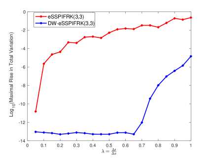
Figure 1: Total variation behavior of the evolution over 25 time-steps evolving the integrating factor methods with the eSSPRK(3,3) Shu-Osher Runge–Kutta method, (2) (red) and with the corresponding method with downwinding (2) (blue). On the x-axis is the value of $\lambda=\frac{\Delta t}{\Delta x}$, on the y-axis is $log_{10}$ of the maximal rise in TV.

For the nonlinear terms, we use a fifth order WENO finite difference method [8]

$$N(u)=WENO\left(-\frac{1}{2}u^{2}\right)\approx-\left(\frac{1}{2}u^{2}\right)_{x}.$$

Although the WENO method is not guaranteed to preserve the total variation behavior, in practice we observe that WENO seems to satisfy

$$\|u^{n}+\Delta tN(u)\|_{TV}\leq\|u^{n}\|_{TV}\;\;\;\;\mbox{for}\;\;\;\Delta t\leq\frac{1}{2}\Delta x$$

for this problem.

For the time discretization, we use the integrating factor method based on the explicit eSSPRK(3,3) Shu-Osher method (3):

$$u^{(1)} = e^{L\Delta t}u^{n}+e^{L\Delta t}\Delta tN(u^{n})$$

$$u^{(2)} = \frac{3}{4}e^{\frac{1}{2}L\Delta t}u^{n}+\frac{1}{4}e^{-\frac{1}{2}L\Delta t}\left(u^{(1)}+\Delta tN(u^{(1)})\right)$$

$$u^{n+1} = \frac{1}{3}e^{L\Delta t}u^{n}+\frac{2}{3}e^{\frac{1}{2}L\Delta t}\left(u^{(2)}+\Delta tN(u^{(2)})\right).$$ (23)

The appearance of negative exponents is due to the fact that the optimal explicit eSSPRK(3,3) Shu-Osher method (3) has decreasing abscissas. These terms threaten to destroy the TVD property.

To correct for these negative values, we use the integrating factor method based on the same explicit eSSPRK(3,3) Shu-Osher method (3),

$$u^{(1)} = e^{L\Delta t}u^{n}+e^{L\Delta t}\Delta tN(u^{n})$$

$$u^{(2)} = \frac{3}{4}e^{\frac{1}{2}L\Delta t}u^{n}+\frac{1}{4}e^{-\frac{1}{2}\tilde{L}\Delta t}\left(u^{(1)}+\Delta tN(u^{(1)})\right)$$

$$u^{n+1} = \frac{1}{3}e^{L\Delta t}u^{n}+\frac{2}{3}e^{\frac{1}{2}L\Delta t}\left(u^{(2)}+\Delta tN(u^{(2)})\right).$$ (24)

but here, whenever the abscissas are decreasing we use a downwinded operator $\tilde{L}\approx 10u_{x}$ defined by

$$\tilde{L}u=-a\left(\frac{u_{j+1}-u_{j}}{\Delta x}\right).$$ (25)

Note that in this case, $\tilde{L}=-L^{T}$. This operator satisfies the TVD condition

$$\|u^{n}-\Delta t\tilde{L}u\|_{TV}\leq\|u^{n}\|_{TV}\;\;\;\;\mbox{for}\;\;\;\Delta t\leq\frac{1}{a}\Delta x.$$

(Again, $a=10$ in our case).

We selected different values of $\Delta t$ and used each one to evolve the solution 25 time steps using the integrating factor Runge–Kutta methods (2) without downwinding and (2) with downwinding. At each stage we calculated the maximal rise in total variation for 25 time steps. In Figure 1 we show the $log_{10}$ of the maximal rise in total variation vs. the value of $\lambda=\frac{\Delta t}{\Delta x}$ of the evolution using the standard integrating factor Runge–Kutta method (2) (in red) and the method with downwinding (2) (in blue). We observe that when downwinding is not used there is a large maximal rise in total variation even for very small values of $\lambda$. However, if we correct for the decreasing abscissas by using the downwinded operator $\tilde{L}$, as in (2), the numerical solution maintains a small maximal rise in total variation up to $\lambda\approx 0.65$.

3 Explicit SSP Runge–Kutta methods

In this section, we present some popular and efficient explicit SSP Runge–Kutta methods. SSP Runge–Kutta methods of various stages and order were reported in [3]. The SSP coefficients of optimal explicit SSP Runge–Kutta methods of up to $s=10$ stages and order $p=4$ are in Table 2. Many of these methods do not feature only non-decreasing abscissas (the second order methods are an exception). In Table 2 we present the corresponding SSP coefficients of the explicit Runge–Kutta methods with non-decreasing abscissas. Unfortunately, no methods of order $p\geq 5$ with positive SSP coefficients can exist [10, 12].

	2	3	4
1	-	-	-
2	1.0000	-	-
3	2.0000	1.0000	-
4	3.0000	2.0000	-
5	4.0000	2.6506	1.5082
6	5.0000	3.5184	2.2945
7	6.0000	4.2879	3.3209
8	7.0000	5.1071	4.1459
9	8.0000	6.0000	4.9142
10	9.0000	6.7853	6.0000

Table 1: SSP coefficients of the optimal eSSPRK(s,p) methods.

	2	3	4
1	-	-	-
2	1.0000	-	-
3	2.0000	0.7500	-
4	3.0000	1.8182	-
5	4.0000	2.6351	1.3466
6	5.0000	3.5184	2.2738
7	6.0000	4.2857	3.0404
8	7.0000	5.1071	3.8926
9	8.0000	6.0000	4.6048
10	9.0000	6.7853	5.2997

Table 2: SSP coefficients of the optimal eSSPRK+(s,p) methods with non-decreasing abscissas.

We use the notation eSSPRK(s,p) to denote an explicit SSP Runge–Kutta method with $s$ stages and of order $p$. As in [7] we use the notation eSSPRK+(s,p) to denote the corresponding method with non-decreasing abscissas. In this paper we consider the Shu-Osher method eSSPRK(3,3) as well as the eSSPRK(4,3), eSSPRK(5,4), and eSSPRK(10,4). We selected these methods by examining the SSP coefficients in Tables 2 and 2 above and selecting the two methods for third order and fourth order for which the SSP coefficient of the eSSPRK+(s,p) method is significantly smaller than the corresponding eSSPRK(s,p) method. In fact, these are good methods to explore as the eSSPRK(3,3) and eSSPRK(10,4) are widely used methods. These methods are given below:

eSSPRK(3,3):

$$u^{(1)} = u^{n}+\Delta tF(u^{n})$$

$$u^{(2)} = \frac{3}{4}u^{n}+\frac{1}{4}u^{(1)}+\frac{1}{4}\Delta tF(u^{(1)})$$

$$u^{n+1} = \frac{1}{3}u^{n}+\frac{2}{3}u^{(2)}+\frac{2}{3}\Delta tF(u^{(2)}).$$ (26)

This method has $\mathcal{C}=1$. The abscissas are

$$(c_{1},c_{2},c_{3})=(0,1,1/2).$$

eSSPRK(4,3):

$$u^{(1)} = u^{n}+\frac{1}{2}\Delta tF(u^{n})$$

$$u^{(2)} = u^{(1)}+\frac{1}{2}\Delta tF(u^{(1)})$$

$$u^{(3)} = \frac{2}{3}u^{n}+\frac{1}{3}\left(u^{(2)}+\frac{1}{2}\Delta tF(u^{(2)})\right)$$

$$u^{n+1} = u^{(3)}+\frac{1}{2}\Delta tF(u^{(3)})$$ (27)

This method has $\mathcal{C}=2$. The abscissas are

$$(c_{1},c_{2},c_{3},c_{4})=(0,1/2,1,1/2).$$

No four stage fourth order explicit Runge–Kutta methods exist with a positive SSP coefficient [4, 12]. However, fourth order methods with more than four stages ($s>p$) do exist. A five stage fourth order method found by Spiteri and Ruuth [16] is
eSSPRK(5,4):

$$u^{(1)} = u^{n}+0.391752226571890\Delta tF(u^{n})$$

$$u^{(2)} = 0.444370493651235u^{n}+0.555629506348765u^{(1)}+0.368410593050371\Delta tF(u^{(1)})$$

$$u^{(3)} = 0.620101851488403u^{n}+0.379898148511597u^{(2)}+0.251891774271694\Delta tF(u^{(2)})$$

$$u^{(4)} = 0.178079954393132u^{n}+0.821920045606868u^{(3)}+0.544974750228521\Delta tF(u^{(3)})$$

$$u^{n+1} = 0.517231671970585u^{(2)}+0.096059710526147u^{(3)}+0.063692468666290\Delta tF(u^{(3)})$$

$$+0.386708617503268u^{(4)}+0.226007483236906\Delta tF(u^{(4)})\,,$$

The abscissas are

$$(c_{1},c_{2},c_{3},c_{4},c_{5})=(0,0.391752226571889,0.586079689311541,0.474542363121399,0.935010630967652).$$

A notable example of a fourth order methods with more than four stages is Ketcheson’s eSSPRK(10,4) that has $\mathcal{C}=6$ and an attractive low storage formulation [9]:
eSSPRK(10,4):

$$u^{(1)} = u^{n}+\frac{1}{6}\Delta tF(u^{n})$$

$$u^{(i+1)} = u^{(i)}+\frac{1}{6}\Delta tF(u^{(i)})\;\;\;i=1,2,3$$

$$u^{(5)} = \frac{3}{5}u^{n}+\frac{2}{5}\left(u^{(4)}+\frac{1}{6}\Delta tF(u^{(4)})\right)$$

$$u^{(i+1)} = u^{(i)}+\frac{1}{6}\Delta tF(u^{(i)})\;\;\;i=5,6,7,8$$

$$u^{n+1} = \frac{1}{25}u^{n}+\frac{9}{25}\left(u^{(4)}+\frac{1}{6}\Delta tF(u^{(4)})\right)+\frac{3}{5}\left(u^{(9)}+\frac{1}{6}\Delta tF(u^{(9)})\right)\,,$$

has $\mathcal{C}=6$. The abscissas are

$$(c_{1},c_{2},c_{3},c_{4},c_{5},c_{6},c_{7},c_{8},c_{9},c_{10})=(0,1/6,1/3,1/2,2/3,1/3,1/2,2/3,5/6,1).$$

These four eSSPRK(s,p) methods have an SSP coefficient that is significantly larger than the corresponding methods with only non-decreasing abscissas, eSSPRK+(s,p), as we can see in Tables 2 and 2. This leads us to expect that for these $(s,p)$ combinations, using the downwinding operator $\tilde{L}$ to salvage the SSP property of the eSSPRK methods would be more efficient than using the corresponding eSSPRK+ method with only non-decreasing coefficients. In the following section, we use these methods in numerical tests and compare their performance.

4 Numerical Results

4.1 Sharpness of SSP time-step

As in the motivating example, we consider Burgers’ equation with a linear advection term

$$U_{t}+10U_{x}+\left(\frac{1}{2}U^{2}\right)_{x} =0\hskip 54.2025ptU(0,x)=\begin{cases}1,&\text{if }1/4\leq x\leq 3/4\\ 0,&\text{else }\end{cases}$$

on the domain $x\in[0,1]$ with periodic boundary conditions. We discretize the spatial grid with $1000$ points and use a first-order upwind difference $Lu\approx-10u_{x}$ defined by (22) to semi-discretize the linear term. As mentioned above, this operator satisfies the TVD condition

$$\|u^{n}+\Delta t{L}u\|_{TV}\leq\|u^{n}\|_{TV}\;\;\;\;\mbox{for}\;\;\;\Delta t\leq\frac{1}{10}\Delta x.$$

When the abscissas decrease, the downwind operator is used instead, as in (2). This downwind operator is defined by (25) and satisfies the TVD condition

$$\|u^{n}-\Delta t\tilde{L}u\|_{TV}\leq\|u^{n}\|_{TV}\;\;\;\;\mbox{for}\;\;\;\Delta t\leq\frac{1}{10}\Delta x.$$

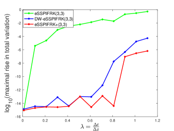
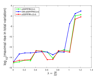
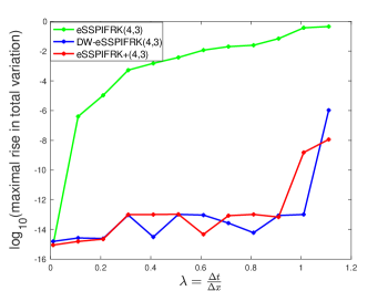
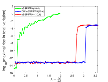
Figure 2: Total variation behavior of the evolution over 25 time-steps evolving the integrating factor methods with the eSSPRK(s,p) Shu-Osher Runge–Kutta method, (green) and with the corresponding method with downwinding (blue), as well as a comparison with the eSSPRK+(s,p) method with non-decreasing abscissas (red). The methods selected are $(s,p)=(3,3),(4,3),(5,4),(10,4)$. On the x-axis is the value of $\lambda=\frac{\Delta t}{\Delta x}$, on the y-axis is $log_{10}$ of the maximal rise in TV.

For the nonlinear terms, we use a fifth order WENO finite difference method [8]

$$N(u)=\frac{1}{2}WENO\left(-u^{2}\right)\approx-\left(\frac{1}{2}u^{2}\right)_{x}$$

. Although the WENO method is not guaranteed to preserve the total variation behavior, in practice we observe that WENO seems to satisfy

$$\|u^{n}+\Delta tN(u)\|_{TV}\leq\|u^{n}\|_{TV}\;\;\;\;\mbox{for}\;\;\;\Delta t\leq\frac{1}{2}\Delta x$$

for this problem.

We measure the total variation of the numerical solution at each stage, and compare it to the total variation at the previous stage. We are interested in the size of time-step $\Delta t$ at which the total variation begins to rise. We refer to this value as the observed TVD time-step. We are interested in comparing this value with the expected TVD time-step dictated by the theory. We call the SSP coefficient corresponding to the value of the observed TVD time-step the observed SSP coefficient $\mathcal{C}_{obs}$. In Figure 2 we show the $log_{10}$ of the maximal rise in total variation versus the ratio $\lambda=\frac{\Delta t}{\Delta x}$, for methods with $(s,p)=(3,3),(4,3),(5,4)$, and $(10,4)$. In each graph, we compare the integrating factor Runge–Kutta using the eSSPRK(s,p) method with and without downwinding, to the integrating factor Runge–Kutta using the eSSPRK+(s,p) method.

The green lines in Figure 2 show that if we do not correct for the decreasing abscissas, the total variation is usually not well-controlled. This is true for the methods with $(s,p)=(3,3),(4,3)$, and $(10,4)$. However, the eSSPRK(5,4) method works well without downwinding, and in fact its performance is identical to that of the eSSPRK+(5,4) method. On the other hand, downwinding negatively impacts the size of the time-step for which the total variation begins to rise. Although the integrating factor approach with eSSPRK(5,4) and downwinding behaves even better than predicted by the theory, the eSSPRK+(5,4) method out-performs the theoretical bound by more [7] . This highlights the fact that while downwinding guarantees that the strong stability property will be preserved when the abscissas decrease, the lack of this guarantee does not always mean that the strong stability property will be violated.

Comparing the blue and red lines in Figure 2 we note that for the $(s,p)=(3,3)$ method, the eSSPRK+(3,3) method with non-decreasing abscissas (red) out-performs the eSSPRK+(3,3) method with downwinding (blue). This may be explained by the fact that this methods performed better than expected: the solution was TVD for larger time-step than predicted by the SSP coefficient (see [7] for a discussion of this behavior).

For the methods with $(s,p)=(4,3)$ and $(s,p)=(10,4)$ we observe in practice the behavior predicted by the theory: when the eSSPRK(s,p) method is not corrected with downwinding (green line), we observe a rise in total variation for any value of $\lambda$. When the integrating factor eSSPRK(s,p) method is corrected with downwinding when the abscissas decrease (blue) the allowable time-step for SSP is larger than for the eSSPIFRK+(s,p) method (red) as predicted by the theory. As we noted in [7], the SSP coefficients of the eSSPRK+(s,p) methods are approximately 10% smaller than those of the eSSPRK(s,p) methods, so the advantage of using downwind over using a method with non-decreasing abscissas is relatively modest. In the case of $(s,p)=(4,3)$ the increase is from $\lambda_{TV}=0.9$ for the method with non-decreasing abscissas to $\lambda_{TV}=1$ for the methods with downwinding, and for $(s,p)=(10,4)$ the increase is from $\lambda_{TV}=2.65$ to $\lambda_{TV}=3$.

4.2 Accuracy studies

Consider the problem

$$U_{t}+U_{x}+\left(\frac{1}{2}U^{2}\right)_{x} =0\hskip 54.2025ptU(0,x)=\frac{1}{2}\left(1+\sin(x)\right)$$ (28)

on the domain $0\leq x\leq 2\pi$. We use the fifth order WENO for the nonlinear term, and upwind finite difference methods to spatially discretize the linear advection term. For the time-discretization we step to final time $T_{f}=1.0$ using an integrating factor Runge–Kutta approach with eSSPRK(3,3) and eSSPRK(10,4) with and without downwinding.

To compute the highly accurate reference solution to the PDE we used $24,000$ points in space and a spectral differentiation operator for the linear advection term with a fifth order WENO for the nonlinear Burgers’ term; for the time evolution we used MATLAB’s embedded ODE45 routine with $AbsTol=10^{-14}$ and $RelTol=5\times 10^{-14}$. In this accuracy test, we have a smooth solution (for the time interval selected), and so the spectral differentiation operator, which does not have the nonlinear stability properties needed for the solution of a problem with discontinuities, will be stable for this smooth problem.

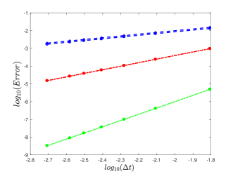
Figure 3: Test 1: Log-log plot of the $L_{2}$ errors vs. the timestep using the integrating factor Runge–Kutta method eSSPRK(s,p) with downwinding (with * markers) and the integrating factor Runge–Kutta method with non-decreasing abscissas eSSPRK+(s,p) (with o markers). The blue line is for the first order spatial operator $L1_{N_{x}}$, the red line is for the second order spatial operator $L2_{N_{x}}$, and the green line for the spectral spatial operator $Lspec_{N_{x}}$. Left: $(s,p)=(3,3)$. Right: $(s,p)=(10,4)$.

Note that the markers look like solid circles because the * markers overlap with the o markers.

Test 1: space-time co-refinement study.
In our first test, we use $N_{x}=[100,200,300,400,500,600,800]$ points in space and a time-step of $\Delta t=\frac{\Delta x}{4}$. For the spatial discretization we use a first order upwind operator $L1_{N_{x}}$, the second order upwind operator $L2_{N_{x}}$, and the spectral operator $Lspec_{N_{x}}$. For each value of $N_{x}$ we compute the error vector and calculate its $L_{2}$ norm. In Figure 3 we compare the convergence of the integrating factor Runge–Kutta method eSSPRK(3,3) with downwinding to the integrating factor Runge–Kutta method with non-decreasing abscissas eSSPRK+(3,3). We observe that when using a low-order spatial discretization $L1_{N_{x}}$ and $L2_{N_{x}}$ for the linear advection term the spatial error is clearly dominating, and the order of convergence is first and second order respectively. The results are the same when we use eSSPRK(10,4) with downwinding and eSSPRK+(10,4). When using the spectral discretization $Lspec_{N_{x}}$ for the linear advection term, we see convergence of order $3.5$. This order is the same for all the methods, whether using the third or fourth order time discretization, so we conclude that here, too, the spatial error dominated.

This first test shows that the integrating factor approach using the optimal SSP Runge–Kutta method while incorporating downwinding converges properly, and its errors are close to identical to the non-decreasing abscissa approach described in [7]. This establishes that, as expected, downwinding is an appropriate technique to employ when dealing with a PDE.

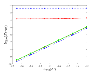
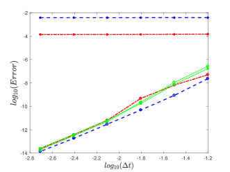
Figure 4: Test 2: log-log plot of the $L_{2}$ errors vs. the timestep using the integrating factor Runge–Kutta method eSSPRK(s,p) with downwinding (with * markers) and the integrating factor Runge–Kutta method with non-decreasing abscissas eSSPRK+(s,p) (with o markers). The blue line is for the first order spatial operator $L1_{50}$, the red line is for the second order spatial operator $L2_{50}$, and the green line for the spectral spatial operator $Lspec_{50}$. Left: $(s,p)=(3,3)$. Right: $(s,p)=(10,4)$. Note that the markers look like solid circles because the * markers overlap with the o markers.

It is important to keep in mind that while the PDE is being approximated equally well whether downwinding is employed or not, this is not the case for convergence to the ODE. This is due to the fact that while the ODE resulting from discretizing (28) with $L$ is

$$u_{t}=Lu+N(u)$$ (29)

the ODE that results from discretizing (28) with $\tilde{L}$ is

$$u_{t}=\tilde{L}u+N(u),$$ (30)

which is a different ODE, with a correspondingly different solution. We perform the following numerical test to see how downwinding impacts the solution to the ODE.

Test 2: ODE convergence study.
We chose $N_{x}=50$ points and discretize the linear advection term using $L1_{50}$, $L2_{50}$, and $Lspec_{50}$. The nonlinear term is computed as above using WENO, but with $N_{x}=50$ points. The reference solution is found by evolving the ODE resulting from this semi-discretization using MATLAB’s embedded ODE45 routine with $AbsTol=10^{-14}$ and $RelTol=5\times 10^{-14}$.

We evolve this semi-discrete ODE using the integrating factor approach based on the eSSPRK(s,p) methods with downwinding for the cases when the abscissas decrease, and using the integrating factor Runge–Kutta methods based on the eSSPRK+(s,p) methods, for $\Delta t=\lambda\Delta x$ where $\lambda=\frac{1}{2},\frac{1}{4},\frac{1}{8},\frac{1}{16},\frac{1}{32},\frac{1}{64}.$ For each value of $\Delta t$ we compute the error vector and calculate its $L_{2}$ norm. We compare the convergence of the integrating factor Runge–Kutta method eSSPRK(s,p) with downwinding to the integrating factor Runge–Kutta method with non-decreasing abscissas eSSPRK+(s,p), for $(s,p)=(3,3),(10,4)$. In Figure 4 we observe that when the number of points in space is fixed and only the time-step is refined, the integrating factor Runge–Kutta method with downwinding has a large error which the solution hangs at about $3.8\times 10^{-3}$ (blue). We repeat this test with a second order upwind operator $L2_{50}$ for the linear advection operator and observe that the solution hangs at about $1.5\times 10^{-4}$ (red). In contrast, the methods without downwinding exhibit the expected order of convergence in time, regardless of the order of the spatial operator. For the spectral operator, $L=\tilde{L}$, so as expected, there is no difference when downwinding is used. (Note that the accuracy results when we use eSSPRK(s,p) without downwinding are similar to those of eSSPRK+(s,p)). This behavior is well-known in problems with downwinding and discussed extensively in [6].

5 Conclusions

In [7] we first considered the strong stability properties of integrating factor Runge–Kutta methods. In that work we presented sufficient conditions for preservation of strong stability for integrating factor Runge–Kutta methods, which required the use of explicit SSP Runge–Kutta methods with non-decreasing abscissas, denoted eSSPRK+ methods. When considering methods of order $p=3,4$ many of the eSSPRK+(s,p) methods have smaller SSP coefficients (and therefore smaller allowable time-step) than the optimal eSSPRK(s,p) methods, which often have some decreasing abscissas.

In this work, we consider a different approach to preserving the strong stability properties of integrating factor Runge–Kutta methods. In this case, when the abscissas of the eSSPRK methods are decreasing, we replace the spatial operator $L$ with a downwinded spatial operator $\tilde{L}$ to preserve the strong stability properties of integrating factor Runge–Kutta method. We presented a complete SSP theory for this approach. However, our numerical examples show that the downwinded spatial operators introduce some errors that may adversely affect the accuracy of the methods, and that in most cases the integrating factor approach with explicit SSP Runge–Kutta methods with non-decreasing abscissas performs nearly as well, if not better, than with explicit SSP Runge–Kutta methods with downwinding. These results lead us to conclude that the downwinding approach may not, in practice, provide much benefit over using explicit SSP Runge–Kutta methods with non-decreasing abscissas, as described in [7].

Acknowledgment. This publication is based on work supported by AFOSR grant FA9550-15-1-0235 and NSF grant DMS-1719698.

References

- [1] S. Conde, S. Gottlieb, Z. Grant, and J.N. Shadid, Implicit and Implicit-Explicit Strong Stability Preserving Runge–Kutta Methods with High Linear Order. Journal of Scientific Computing 73(2) (2017), pp. 667-690.
- [2] S. Cox and P. Matthews, Exponential time differencing for stiff systems, Journal of Computational Physics, 176 (2002), pp. 430–455.
- [3] S. Gottlieb, D. I. Ketcheson, and C.-W. Shu, Strong Stability Preserving Runge–Kutta and Multistep Time Discretizations, World Scientific Press, 2011.
- [4] S. Gottlieb and C.-W. Shu, Total variation diminishing runge–kutta methods, Mathematics of Computation, 67 (1998), pp. 73–85.
- [5] S. Gottlieb, C.-W. Shu, and E. Tadmor, Strong Stability Preserving High-Order Time Discretization Methods, SIAM Review, 43 (2001), pp. 89–112.
- [6] I. Higueras, D. I. Ketcheson, and T. A. Kocsis, Optimal monotonicity-preserving perturbations of a given Runge-Kutta method, Journal of Scientific Computing (2018).
- [7] L. Isherwood, S. Gottlieb, and Z. Grant, Strong Stability Preserving Integrating Factor Runge–Kutta Methods. arXiv:1708.02595 (2017).
- [8] G.-S. Jiang, and C.-W. Shu, Efficient Implementation of Weighted ENO Schemes, Journal of Computational Physics, 126 (1996), pp. 202-228.
- [9] D. I. Ketcheson, Highly efficient strong stability preserving Runge–Kutta methods with low-storage implementations, SIAM Journal on Scientific Computing, 30 (2008), pp. 2113–2136.
- [10] J. F. B. M. Kraaijevanger, Contractivity of Runge–Kutta methods, BIT, 31 (1991), pp. 482–528.
- [11] J. D. Lawson, Generalized Runge-Kutta Processes for Stable Systems with Large Lipschitz Constants, SIAM Journal on Numerical Analysis, 4(3) (1967), 372–380.
- [12] S. J. Ruuth and R. J. Spiteri, Two barriers on strong-stability-preserving time discretization methods, Journal of Scientific Computation, 17 (2002), pp. 211–220.
- [13] C.-W. Shu, Total-variation diminishing time discretizations, SIAM Journal Scientific Statistical Computing, 9 (1988), pp. 1073–1084.
- [14] C.-W. Shu and S. Osher, Efficient implementation of essentially non-oscillatory shock-capturing schemes, Journal of Computational Physics, 77 (1988), pp. 439–471.
- [15] M. Spijker, Stepsize conditions for general monotonicity in numerical initial value problems, SIAM Journal on Numerical Analysis, 45 (2008), pp. 1226–1245.
- [16] R. J. Spiteri and S. J. Ruuth, A new class of optimal high-order strong-stability-preserving time discretization methods, SIAM Journal on Numerical Analysis, 40 (2002), pp. 469–491.