Optimal Impulse Control of SIR Epidemics over Scale-Free Networks

Abstract

Recent wide spreading of Ransomware has created new challenges for cybersecurity over large-scale networks. The densely connected networks can exacerbate the spreading and makes the containment and control of the malware more challenging. In this work, we propose an impulse optimal control framework for epidemics over networks. The hybrid nature of discrete-time control policy of continuous-time epidemic dynamics together with the network structure poses a challenging optimal control problem. We leverage the Pontryagin’s minimum principle for impulsive systems to obtain an optimal structure of the controller and use numerical experiments to corroborate our results.

1 Introduction

Malware spreading becomes a more prevalent issue recently as the number of devices and their connections grow exponentially. Many devices that are connected to the Internet do not have strong protections, and they contain cyber vulnerabilities that create a fast spreading of malware over large networks. A higher level of connectivity of the network is often desired for information spreading. However, in the context of malware, the high connectivity can exacerbate the spreading and makes the containment and control of the malware more challenging. One example is the recent Ransomware Ransomware ; Luo that spreads over the Internet with the objective to lock the files of a victim using cryptographic techniques and demand a ransom payment to decrypt them. The worldwide spread of WannaCry ransomware has affected more than 200,000 computers across 150 countries and caused billions of dollars of damages. Hence it is critical to take into account the network structure when developing control policies to control the infection dynamics.

In this paper, we investigate a continuous-time Susceptible-Infected-Recovered (SIR) epidemic model over large-scale networks. The malware control mechanism is to patch an optimal fraction of the infected nodes at discrete points in time. Such mechanism is also known as an optimal impulse controller. The hybrid nature of discrete-time control policy of continuous-time epidemic dynamics together with the network structure poses a challenging optimal control problem. We leverage the Pontryagin’s minimum principle for impulsive systems to obtain an optimal structure of the controller and use numerical experiments to demonstrate the computation of the optimal control and the controlled dynamics. This work extends the investigation of previous related works Zhu ; Gubar ; Taynitskiy to a new paradigm of coupled epidemic models and the regime of optimal impulsive control.

The rest of the paper is organized as follows. Section II presents the controlled SIR mathematical model. Section III shows the structure of optimal control policies. Section IV presents numerical examples. Section V concludes the paper.

2 The model

In this section, we formulate a model of spreading of malware in the network of $N$ nodes use the modification of classical SIR model. As in previous works Gubar , Taynitskiy:2016 two different forms of malware with different strengths spread over the network simultaneously, we denote them as $M_{1}$ and $M_{2}$. We also assume that a structure of population is described by the scale free network Vespignani , Porokhnyavaya . Normally, as SIR model points, all nodes in the population are divided into three groups: Susceptible $(S)$, Infected $(I)$ and Recovered $(R)$, Altman. Susceptible is a group of nodes which are not infected by any malware, but may be invaded by any forms of virus. The Infected nodes are those that have been attacked by the virus and the Recovered is a group of recovered nodes. In modified model subgroup of Infected nodes also is brunched into two subgroups $I_{1}$ and $I_{2}$, where nodes in $I_{i}$ are infected by malware $M_{i},i=1,2$ respectively. We formulate the epidemic process as a system of nonlinear differential equations, where $n_{S}$, $n_{M_{1}}$, $n_{M_{2}}$ and $n_{R}$ correspond to the number of susceptible, infected and recovered nodes, respectively. In current model the connections between nodes are described by the scale-free network, then we will use the following notation: $S_{k}(t)$ and $R_{k}(t)$ are fractions of Susceptible and Recovered nodes with degree $k$ at time moment $t$, $I^{1}_{k}(t),I^{2}_{k}(t)$ are fractions of Infected nodes with degree $k$. At each time moment $t\in[0,T]$ the number of nodes is constant and equal $N$, and the following condition $S_{k}(t)+I^{1}_{k}(t)+I^{2}_{k}(t)+R_{k}(t)=1$ is satisfied. The process of spreading is defined by the system of ordinary differential equations:

$$\begin{array}[]{l}\displaystyle\frac{dS_{k}}{dt}=-\delta_{1k}S_{k}I^{1}_{k}\Theta_{1}-\delta_{2k}S_{k}I^{2}_{k}\Theta_{2};\\ \displaystyle\frac{dI^{1}_{k}}{dt}=\delta_{1k}S_{k}I^{1}_{k}\Theta_{1}-\sigma^{1}_{k}I^{1}_{k};\\ \displaystyle\frac{dI^{2}_{k}}{dt}=\delta_{2k}S_{k}I^{2}_{k}\Theta_{2}-\sigma^{2}_{k}I^{2}_{k},\\ \displaystyle\frac{dR_{k}}{dt}=\sigma^{1}_{k}I^{1}_{k}+\sigma^{2}_{k}I^{2}_{k},\end{array}$$ (1)

where $\delta_{ik}(k)$ is the infections rate for the first type of malware $i$ if a susceptible node has a contact with infected node with the degree $k$, $\sigma^{i}_{k}$ is recovery rate.

We consider the graph generated by using the algorithm devised in barabasi . We start from a small number $m_{0}$ of disconnected nodes; every time step a new node is added, with $m$ links that are connected to an old node $i$ with $k_{i}$ links according to the probability $k_{i}/\sum_{j}k_{j}$. After iterating this scheme a sufficient number of times, we obtain a network composed by $N$ nodes with connectivity distribution $P(k)\approx k^{-3}$ and average connectivity $\langle k\rangle=2m$. In this work we take $m=4$.

At the initial time moment $t=0$, the most number of nodes belong to Susceptible group and only a small fraction of Infected by malwares $M_{1}$ or $M_{2}$. Initial state for system (1) is $0<S_{k}(0)<1$, $0<I^{1}_{k}(0)<1$, $0<I^{2}_{k}(0)<1$, $R(0)=1-S_{k}(0)-I^{1}_{k}(0)-I^{2}_{k}(0)$. Analogously with Fu , Vespignani we define parameter $\Theta_{i}(t)$ as

$$\Theta_{i}(\lambda_{i})=\sum\limits_{k^{\prime}}\frac{\delta_{ik}P(k^{\prime}|k)I^{i}_{k^{\prime}}}{k^{\prime}},\ i=1,2,$$ (2)

where $\delta_{ik}$ denotes the infectivity of a node with degree $k$ and $\lambda_{i}=\delta_{ik}/\sigma^{i}_{k}$ an effective spreading rate. $P(k^{\prime}|k)$ describes the probability of a node with degree $k$ pointing to a node with degree $k^{\prime}$, and $P(k^{\prime}|k)=\frac{k^{\prime}P(k^{\prime})}{k^{\prime}}$, where $\langle k\rangle=\sum\limits_{k^{\prime}}kP(k)$. For scale-free node distribution $P(k)=C^{-1}k^{-2-\gamma},\ 0<\gamma\leq 1$, where $C=\zeta(2+\gamma)$ is Riemann’s zeta function, which provides an appropriate normalization constant for sufficiently large networks. In the SF model considered here, we have a connectivity distribution $P(k)=2m^{2}/k^{-3}$, where $k$ is approximated as a continuous variable. According to Vespignani we can rewrite (2) as

$$\Theta_{i}(\lambda_{i})=\frac{e^{-1/m\lambda_{i}}}{m\lambda_{i}},\ i=1,2.$$ (3)

3 Impulse control problem

Previously it was shown in Vespignani a small fraction of the infected nodes might be survived on small segments of the network and can provoke new waves of epidemics. This cycled process recalls the behavior the virus of influenza which causes a seasonally periodic epidemic, Agur . Hence the control of the epidemic process can be formulated as an impulse control problem in which a series of impulses of antivirus patches are designed to reduce the periodically incipient zones of infected nodes. We extend the model (1) to present an impulse control problem for episodic attacks of the malware and obtain the optimal strategy of application of antivirus software to damp the spreading of malware at discrete time moments.

We suppose that impulses occur at time $\tau^{i}_{k,1},\ldots,\tau^{i}_{k,q_{i}(k)}$, where $q_{i}(k)$ describes the number of launching of impulse controls for nodes with $k$ degrees, index $i$ indicates the type of malware. We also assume that on the time intervals $(\tau^{i}_{k,j},\tau^{i}_{k,j+1}]$ system (1) describes the behavior of malware in the network. We have reformulated epidemic model to describe the situation with two types of malware for all time periods except the sequence of times $\tau_{k,j}^{i+}$, $j=1,\ldots,q_{i}(k)$, $i=1,2$. Additionally, we set $S(\tau_{k,j}^{i})=S(\tau_{k,j}^{i-})$, $I_{1}(\tau_{k,j}^{i})=I_{1}(\tau_{k,j}^{i-})$, $I_{2}(\tau_{k,j}^{i})=I_{2}(\tau_{k,j}^{i-})$, $R(\tau_{k,j}^{i})=R(\tau_{k,j}^{i-})$.

The system after activation of impulses at time moment $\tau_{k,j}^{i+}$ is:

$$\begin{array}[]{l}S_{k}(\tau_{k,j}^{i+})=S_{k}(\tau_{k,j}^{i}),\\ {I^{1}_{k}}({\tau_{k,j}^{i+}})=I^{1}_{k}(\tau_{k,j}^{i})-\nu^{1}_{k}(\tau_{k,j}^{i}),\\ {I^{2}_{k}}({\tau_{k,j}^{i+}})=I^{2}_{k}(\tau_{k,j}^{i})-\nu^{2}_{k}(\tau_{k,j}^{i}),\\ {R_{k}}({\tau_{k,j}^{i+}})={R_{k}}(\tau_{k,j}^{i})+\nu^{1}_{k}(\tau_{k,j}^{i})+\nu^{2}_{k}(\tau_{k,j}^{i}).\end{array}$$ (4)

Variables $\nu^{i}_{k}=({\nu^{i}_{k,1}},\ldots,{\nu^{i}_{k,q_{i}(k)}})$, $i=1,2,$ correspond to control impulses applied at the discrete time moments $\tau_{k,1},\ldots,\tau_{k,q_{i}(k)}$ and represent the fraction of recovered nodes. Let be $\nu^{i}_{k,j}={c^{i}_{k,j}}\delta(t-{\tau^{i}_{k,j}})$, where $\delta(t-{\tau^{i}_{k,j}})$ is Dirac function, ${c^{i}_{k,j}}\in[0,{\overline{u}^{i}_{k,j}}]$ is the value of impulse, leads to changes of the dynamical system, ${\overline{u}^{i}_{k,j}}$ is the maximum value for control Agur .

Functional: the objective function of the combined system (4) is represented by the aggregated costs on the time interval $[0,T]$ including the costs of control impulses. The aggregated costs for continuous system (1) are defined as follows: at time moment $t\neq{\tau^{i}_{k,j}},\ j=1,\ldots,q_{i}(k)$, $i=1,2$, we have the costs from infected nodes $f^{1}_{k}(I^{1}_{k}(t))$ and $f^{2}_{k}(I^{2}_{k}(t))$. Functions $f^{i}_{k}(\cdot)$ are non-decreasing and twice-differentiable, such that $f^{i}_{k}(0)=0$, $f^{i}_{k}(I^{i}_{k}(t))>0$ for $I^{i}_{k}(t)>0$ with $t\in({\tau^{i}_{k,j-1}},{\tau^{i}_{k,j}}]$. For system (4), we define the treatment costs as functions $h^{i}_{k}(\nu^{i}_{k,j}({\tau^{i+}_{k,j}}))$, $j=1,\ldots,{q_{i}(k)}$, where $h^{i}_{k}(\nu^{i}_{k,j}({\tau^{i+}_{k,j}}))>0$, $\nu^{i}_{k,j}({\tau^{i+}_{k,j}})>0$ for $i=1,2$. Functions $g(R_{k}(t))$ are non-decreasing and capture the benefit rates from Recovered nodes. The aggregated system costs are defined by the functional:

$$\begin{array}[]{l}J=\sum\limits_{k\in\mathbb{N}}[\int_{0}^{T}f^{1}_{k}(I^{1}_{k}(t))+f^{2}_{k}(I^{2}_{k}(t))-g(R(t))dt+\\ \hskip 40.0pt\sum\limits_{j=1}^{q_{1}(k)}h^{1}_{k}(\nu^{1}_{k,j}({\tau^{1}_{k,j}}))+\sum\limits_{j=1}^{q_{2}(k)}h^{2}_{k}(\nu^{2}_{k,j}({\tau^{2}_{k,j}}))].\end{array}$$ (5)

4 The structure of impulse control

According to principle maximum in impulse form Blaquiere , Chahim , Dykhta , Taynitskiy we write Hamiltonian for dynamic system (1)

$$\begin{array}[]{l}H^{0}_{k}(t)=-(f^{1}_{k}(I^{1}_{k}(t))+f^{2}_{k}(I^{2}_{k}(t))-g(R_{k}(t)))+(\lambda_{I^{1}_{k}}(t)-\lambda_{S_{k}}(t))\delta_{1k}S_{k}(t)I^{1}_{k}(t)\Theta_{1}(t)+\\ \hskip 35.0pt(\lambda_{I^{2}_{k}}(t)-\lambda_{S_{k}}(t))\delta_{2k}S_{k}(t)I^{2}_{k}(t)\Theta_{2}(t)+(\lambda_{R_{k}}-\lambda_{I^{1}_{k}})\sigma^{1}_{k}I^{1}_{k}+(\lambda_{R_{k}}-\lambda_{I^{2}_{k}})\sigma^{2}_{k}I^{2}_{k};\end{array}$$ (6)

and construct adjoint system as follows:

$$\begin{array}[]{l}\displaystyle\dot{\lambda}_{S_{k}}(t)=(\lambda_{S_{k}}(t)-\lambda_{I^{1}_{k}}(t))\delta_{1k}I^{1}_{k}(t)\Theta_{1}(t)+(\lambda_{S_{k}}(t)-\lambda_{I^{2}_{k}}(t))\delta_{2k}I^{2}_{k}(t)\Theta_{2}(t);\\ \displaystyle\dot{\lambda}_{I^{1}_{k}}(t)=\frac{df^{1}_{k}(I^{1}_{k}(t))}{dI^{1}_{k}}+(\lambda_{S_{k}}(t)-\lambda_{I^{1}_{k}}(t))\left(\delta_{1k}S_{k}(t)\Theta_{1}(t)+\frac{(\delta_{1k})^{2}S_{k}(t)I^{1}_{k}(t)P(k)}{\langle k\rangle}\right)+\\ \hskip 35.0pt(\lambda_{I^{1}_{k}}-\lambda_{R_{k}})\sigma^{1}_{k};\\ \displaystyle\dot{\lambda}_{I^{2}_{k}}(t)=\frac{df^{2}_{k}(I^{2}_{k}(t))}{dI^{2}_{k}}+(\lambda_{S_{k}}(t)-\lambda_{I^{2}_{k}}(t))\left(\delta_{2k}S_{k}(t)\Theta_{2}(t)+\frac{(\delta_{2k})^{2}S_{k}(t)I^{2}_{k}(t)P(k)}{\langle k\rangle}\right)+\\ \hskip 35.0pt(\lambda_{I^{2}_{k}}-\lambda_{R_{k}})\sigma^{2}_{k};\\ \displaystyle\dot{\lambda}_{R_{k}}(t)=-\frac{dg(R_{k}(t)}{dR_{k}},\end{array}$$ (7)

with transversality conditions $\lambda_{S_{k}}(T)=\lambda_{I^{1}_{k}}(T)=\lambda_{I^{2}_{k}}(T)=\lambda_{R_{k}}(T)=0$.

Following the maximum principle for impulse control (see Blaquiere , Sethi , Chahim ), we formulate necessary optimality conditions as in Theorem 4.1.

Theorem 4.1

Let $(x^{*},N,\tau_{i}^{j*},\nu_{i}^{*})$, $i=1,2,$ be an optimal solution for the impulse control problem. Then, there exists an adjoint vector function $\lambda(t)=(\lambda_{S}(t),\lambda_{I_{1}}(t),\lambda_{I_{2}}(t)$, $\lambda_{R}(t))$ such that the following conditions hold:

$$\begin{array}[]{l}\dot{\lambda}_{x}(t)=-\frac{\partial H_{0}}{\partial x}(x^{*}(t),\lambda(t),t),\end{array}$$ (8)

where $x(t)={S(t),I_{1}(t),I_{2}(t),R(t)}$.

At the impulse or jump points, it holds that

$$\begin{array}[]{l}\frac{\partial H_{i}^{c}}{\partial\nu_{i}}(x^{*}(\tau_{i}^{j*-}),\nu_{i},\lambda(\tau_{i}^{j*+}),\tau_{i}^{j*})(\nu_{i}^{j}-\nu_{i}^{j*})\geq 0,\\ \\ \end{array}$$ (9)

$$\begin{array}[]{l}\lambda_{x}(\tau_{i}^{j*+})-\lambda_{x}(\tau_{i}^{j*-})=\frac{\partial H_{i}^{c}}{\partial x}(x^{*}(\tau_{i}^{j*-}),\nu_{i}^{j*},\lambda(\tau_{i}^{j*+}),\tau_{i}^{j*}),\\ \\ \end{array}$$ (10)

$$\begin{array}[]{l}H_{0}(x^{*}(\tau_{i}^{j*+}),\lambda(\tau_{i}^{j*+}),\tau_{i}^{j*})-H_{0}(x^{*}(\tau_{i}^{j*-}),\lambda(\tau_{i}^{j*-}),\tau_{i}^{j*})-\vskip 12.0pt plus 4.0pt minus 4.0pt\\ \hskip 1.0pt-\frac{\partial H_{i}^{c}}{\partial\tau_{i}^{j}}(x^{*}(\tau_{i}^{j*-}),\nu_{i}^{j*},\lambda(\tau_{i}^{j*+}),\tau_{i}^{j*})\par\begin{cases}>0&\text{for $\tau_{i}^{j*}=0$},\\ =0&\text{for $\tau_{i}^{j*}\in(0,T)$,}\\ <0&\text{for $\tau_{i}^{j*}=T$.}\\ \end{cases}\end{array}$$ (11)

For all points in time at which there is no jump, i.e. $t\neq\tau_{j}\ (j=1,\ldots,k_{i})$, it holds that

$$\begin{array}[]{l}\frac{\partial H_{j}^{c}}{\partial\nu_{j}}(x^{*}(t),0,\lambda(t),t)\nu_{j}\leq 0,\end{array}$$ (12)

with the transversality condition $\lambda(T)=0.$

Hamiltonian in impulsive form is

$$\begin{array}[]{l}H^{c}_{k}(\tau_{k,j}^{1+})=-h^{1}_{k}(\nu^{1}_{k,j}(\tau_{k,j}^{1+}))+(\lambda_{R_{k}}(\tau_{k,j}^{1+})-\lambda_{I^{1}_{k}}(\tau_{k,j}^{1+}))\nu^{1}_{k,j}(\tau_{k,j}^{1+});\\ H^{c}_{k}(\tau_{k,j}^{2+})=-h^{2}_{k}(\nu^{2}_{k,j}(\tau_{k,j}^{2+}))+(\lambda_{R_{k}}(\tau_{k,j}^{2+})-\lambda_{I^{2}_{k}}(\tau_{k,j}^{2+}))\nu^{2}_{k,j}(\tau_{k,j}^{2+}).\end{array}$$ (13)

Here we assume that for each type of malwares $M_{1}$ and $M_{2}$ and for each $k$ we have own set of control impulses $\nu^{1}_{k}=({\nu^{1}_{k,1}},\ldots,{\nu^{1}_{k,q_{1}(k)}})$ and $\nu^{2}_{k}=({\nu^{2}_{k,1}},\ldots,{\nu^{2}_{k,q_{2}(k)}})$.

Adjoin system for system(4) is ($i=1,2$):

$$\begin{array}[]{l}\displaystyle\lambda_{S_{k}}(\tau_{k,j}^{i+})=\lambda_{S_{k}}(\tau_{k,j}^{i});\\ \displaystyle\lambda_{I^{1}_{k}}(\tau_{k,j}^{i+})=\lambda_{I^{1}_{k}}(\tau_{k,j}^{i});\\ \displaystyle\lambda_{I^{2}_{k}}(\tau_{k,j}^{i+})=\lambda_{I^{2}_{k}}(\tau_{k,j}^{i});\\ \displaystyle\lambda_{R_{k}}(\tau_{k,j}^{i+})=\lambda_{R_{k}}(\tau_{k,j}^{i}).\end{array}$$ (14)

Here is the conditions for $\Delta_{i}$ for each $I^{i}_{k}$ from the theorem 4.1:

$$\begin{array}[]{l}\displaystyle\Delta_{1}=f^{1}_{k}(I^{1}_{k}(\tau_{k,j}^{1}))-f^{1}_{k}(I^{1}_{k}(\tau_{k,j}^{1+}))-g(R_{k}(\tau_{k,j}^{1}))+g(R_{k}(\tau_{k,j}^{1+}))+\\ \hskip 23.0pt\displaystyle c^{1}_{k,j}[\frac{dg(R_{k}(\tau_{k,j}^{1+}))}{dR_{k}(\tau_{k,j}^{1+})}+\frac{df^{1}_{k}(I^{1}_{k}(\tau_{k,j}^{1+}))}{dI^{1}_{k}(\tau_{k,j}^{1+})}]+2\sigma^{1}_{k}c^{1}_{k,j}(\lambda_{R_{k}}(\tau_{k,j}^{1+})-\lambda_{I^{1}_{k}}(\tau_{k,j}^{1+}))\\ \hskip 23.0pt\displaystyle\delta_{1k}S_{k}(\tau_{k,j}^{1})c^{1}_{k,j}(\lambda_{S_{k}}(\tau_{k,j}^{1})-\lambda_{I^{1}_{k}}(\tau_{k,j}^{1}))[2\Theta_{1}(\tau_{k,j}^{1+})+\frac{\delta_{1k}P(k)}{\langle k\rangle}(1+I^{1}_{k}(\tau_{k,j}^{1})-c^{1}_{k,j})].\end{array}$$ (15)

Here is the conditions for $\Delta$ for each $\Delta$ for each $I^{2}_{k}$ from theorem 4.1:

$$\begin{array}[]{l}\displaystyle\Delta_{2}=f^{2}_{k}(I^{2}_{k}(\tau_{k,j}^{2}))-f^{2}_{k}(I^{2}_{k}(\tau_{k,j}^{2+}))-g(R_{k}(\tau_{k,j}^{2}))+g(R_{k}(\tau_{k,j}^{2+}))+\\ \hskip 23.0pt\displaystyle c^{2}_{k,j}[\frac{dg(R_{k}(\tau_{k,j}^{2+}))}{dR_{k}(\tau_{k,j}^{2+})}+\frac{df^{2}_{k}(I^{2}_{k}(\tau_{k,j}^{2+}))}{dI^{2}_{k}(\tau_{k,j}^{2+})}]+2\sigma^{2}_{k}c^{2}_{k,j}(\lambda_{R_{k}}(\tau_{k,j}^{2+})-\lambda_{I^{2}_{k}}(\tau_{k,j}^{2+}));\\ \hskip 23.0pt\displaystyle\delta_{2k}S_{k}(\tau_{k,j}^{2})c^{2}_{k,j}(\lambda_{S_{k}}(\tau_{k,j}^{2})-\lambda_{I^{2}_{k}}(\tau_{k,j}^{2}))[2\Theta_{2}(\tau_{k,j}^{2+})+\frac{\delta_{2k}P(k)}{\langle k\rangle}(1+I^{2}_{k}(\tau_{k,j}^{2})-c^{2}_{k,j})].\end{array}$$ (16)

According to Theorem 4.1 at time $\tau^{i}_{k,j}\in(0,T)$ $\Delta_{i}$ should be equal to zero. Therefore, we deal with two different problems: firstly, if the intensity of impulses $c^{i}_{k,j}$ are fixed, then from (15) and (16), we can find the optimal time $\tau^{i*}_{k,j}$ of using impulses; secondly, if the sequence of time $\tau^{i}_{k,j}$ are fixed, then we obtain the optimal level of the intensity of impulses $c^{i*}_{k,j}$, $j=1,\ldots,q_{i}$, $i=1,2$.

5 Numerical simulations

In this paragraph we present numerical experiments to depict theoretical results and to study the behavior of malwares and show the application of control impulses. Here we use the following set of the initial states and values of parameters of the system (1): initial system states and parameters are $S_{k}(0)=0.4,$ $I^{1}_{k}(0)=0.3,$ $I^{2}_{k}(0)=0.2$ and $R_{k}(0)=0$, spreading rates are $\delta_{1k}=0.075k$, $\delta_{2k}=0.1k$, self-recovery rates are $\sigma^{1}_{k}=0.0005k$ and $\sigma^{1}_{k}=0.0003k$. We set costs functions for infectious subgroups as $f^{i}_{k}(I^{i}_{k}(t))=A^{i}_{k}I^{i}_{k}(t)$ with coefficients $A^{1}_{k}=2k$, $A^{2}_{k}=3k$ and treatment costs functions as $h^{i}_{k}(\nu^{i}_{k,j}(\tau^{i+}_{k,j})=B^{i}_{k}c^{i}_{k,j}I^{i}_{k}(\tau^{i+}_{k,j})$, where coefficients are equal to $B^{1}_{k}=3k$, $B^{2}_{k}=4k$, $c^{1}_{k,j}=0.1$, $c^{2}_{k,j}=0.08$ for $i=1,2$, utility function is $g(R_{k}(t))=0.1R_{k}(t)$.

Case 1. In case 1 we present the initial example of the behavior of the system and aggregated system costs if an average number of links between $i$-th node and its neighbors is $k=4$. Figs. 1-2 show the spreading on two modification of malwares and corresponding total system costs.

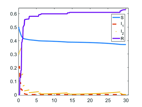
Figure 1: Evolution of the system in Case 1. Number of links: $k=4$, spreading rates: $\delta_{1k}=0.075k$ and $\delta_{2k}=0.1k$.

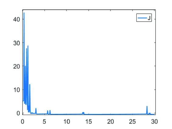
Figure 2: Aggregated system costs are equal to $J=37.65$.

Aggregated system costs in this case are equal to $J=37.65$. By applying the control impulses at discrete time moments we received that an amount of impulses are equal to $p_{1}(4)=37$ and $p_{2}(4)=49$.

Case 2. In this experiment we use the same parameters for initial data, but in contrast tot xase 1 an average number on neighbors is equal $k=7$. In this case, we obtain that the aggregated costs are $J=73.93$, and an amount of impulses are equal to $p_{1}(7)=29$ and $p_{2}(7)=44$. We may notice that increasing the number of neighbor links increases the costs of the system. Since there are less nodes with connectivity $k=7$ which is more than average connectivity $\langle k\rangle=4$, we need less impulse treatment to vaccinate the network, thereby if we apply control to more connected nodes we reduce the costs of treatment.

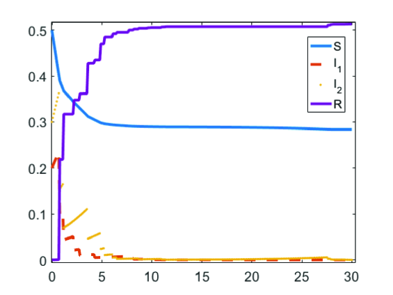
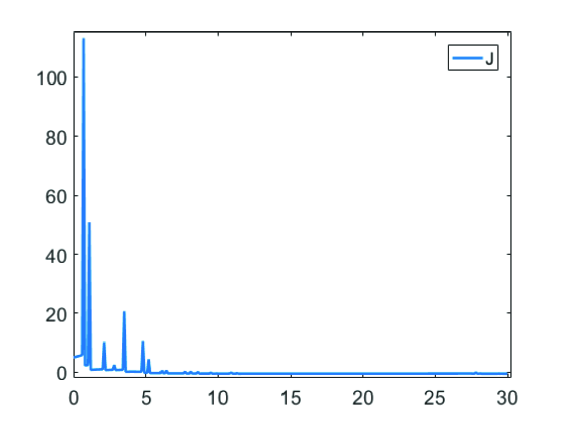
Figure 3: 3 Evolution of the system in Case 2. Number of links: $k=7$, spreading rates: $\delta_{1k}=0.075k$ and $\delta_{2k}=0.1k$. 3 Aggregated system costs are equal to $J=73.93$.

Case 3. In case 3, by using the same initial set of data we variate the spreading rate for malwares and consider $\delta_{1k}=0.075k$ and $\delta_{2k}=0.1k$. Here we receive that the aggregated costs are $J=122.27$ and a number of impulses are $p_{1}(4)=43$ and $p_{2}(4)=55$, then increasing the spreading rates are leading to increasing aggregated costs and number of impulses which are needed to heal the network.

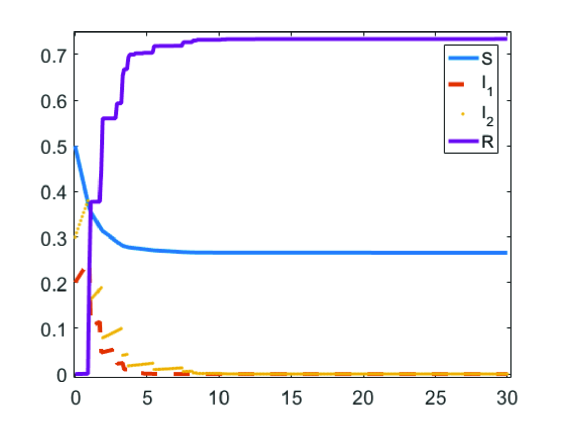
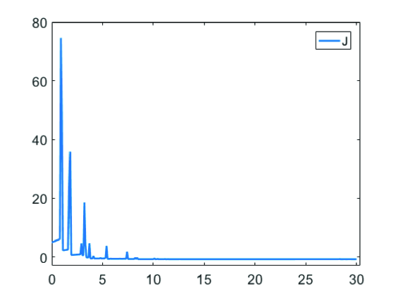
Figure 4: 4 Evolution of the system in Case 3. Number of links: $k=4$, spreading rates: $\delta_{1k}=0.1k$ and $\delta_{2k}=0.2k$. 4 Aggregated system costs are equal to $J=122.27$.

6 conclusion

This work addresses the spreading of cyber threats over large-scale networks by investigating the optimal control policies in the impulsive form for SIR-type of epidemics over scale-free networks. We have applied the impulse optimal control framework to the epidemics over networks to devise impulsive protection policies to mitigate the impact of the epidemics and contain the spreading of the malware. With the application of the maximum principle, we have obtained the structure of the optimal control impulses where actions are taken at discrete-time moments. We have corroborated the obtained results using numerical examples.

References

• (1) Kharraz, A., Robertson, W., Balzarotti, D., Bilge, L., Kirda, E, Cutting the gordian knot: A look under the hood of ransomware attacks. In International Conference on Detection of Intrusions and Malware, and Vulnerability Assessment, pp. 3-24. Springer, 2015.
• (2) Blaqui$\grave{e}$re A. Impulsive Optimal Control with Finite or Infinite Time Horizon. Journal Of Optimization Theory And Applications., vol. 46. 1985.
• (3) Chahim, M., Harti, R., Kort, P. A tutorial on the deterministic Impulse Control Maximum Principle: Necessary and sufficient optimality conditions. European Journal of Operational Research., 219, 18–26, 2012.
• (4) Dykhta V. A., Samsonyuk O. N. A maximum principle for smooth optimal impulsive control problems with multipoint state constraints. Computational Mathematics and Mathematical Physics., 49, 942–957, 2009.
• (5) Taynitskiy V., Gubar E., Zhu Q. Optimal Impulse Control of Bi-Virus SIR Epidemics with Application to Heterogeneous Internet of Things. Constructive Nonsmooth Analysis and Related Topics. Abstracts of the International Conference. Dedicated to the Memory of Professor V.F. Demyanov. p. 113-116, 2017.
• (6) Barab si, A. L., Albert, R. Emergence of scaling in random networks. science, 286(5439), pp. 509-512, 1999.
• (7) Gubar E., Zhu Q., Taynitskiy V. Optimal Control of Multi-strain Epidemic Processes in Complex Networks. Game Theory for Networks. GameNets 2017. Lecture Notes of the Institute for Computer Sciences, Social Informatics and Telecommunications Engineering, vol 212. Springer, Cham. p. 108–117, 2017.
• (8) Gubar E., Kumacheva S., Zhitkova E., Porokhnyavaya O. Impact of Propagation Information in the Model of Tax Audit. Recent Advances in Game Theory and Applications. ”Static and Dynamic Game Theory: Foundations and Applications”. Switzerland. p. 91–110, 2015.
• (9) Fu X., Small M., Walker D. M., Zhang H. Epidemic dynamics on scale-free networks with piecewise linear infectivity and immunization. Phys. Rev. E. 77, 3, 036113, 2008.
• (10) Pastor-Satorras R., Vespignani A. Epidemic spreading in scale-free networks. Phys. Rev. Lett. 86, 14, 3200, 2001.
• (11) Agur Z., Cojocaru L., Mazor G., Anderson R. M., Danon Y. L. Pulse mass measles vaccination across age cohorts. Proceedings of the National Academy of Sciences of the United States of America. 90:11698–11702, 1993.
• (12) Luo X, Liao Q. Ransomware: A new cyber hijacking threat to enterprises. Handbook of research on information security and assurance. 2009:1-6.
• (13) Masuda N., Konno N. Multi-state epidemic processes on complex networks. J. Theor. Biol.243, 1, 64–75, 2006.
• (14) Sethi, S.P., Thompson, G.L. Optimal Control Theory: Applications to Management Science and Economics. Springer, Berlin, 2006.
• (15) Taynitskiy V. A., Gubar E. A., Zhitkova E. M. Optimization of protection of computer networks against malicious software, Proc. of International Conference ”Stability and Oscillations of Nonlinear Control Systems” (Pyatnitskiy’s Conference), 2016.
• (16) Zaccour, G., Reddy, P., Wrzaczek, S. Quality effects in different advertising models - An impulse control approach. European Journal of Operational Research., 255, 984–995, 2016.
• (17) Leander R., Lenhart S. and Vladimir Protopopescu V. Optimal control of continuous systems with impulse controls. Optimal Control Applications and Methods Optim. Control Appl. Meth., 36:–549, 2015.
• (18) Gubar, E., Zhu, Q. Optimal Control of Influenza Epidemic Model with Virus Mutations. Proceedings 12th Biannual European Control Conference. IEEE Control Systems Society. 3125–3130, 2013.