An edge-based pressure stabilisation technique for finite elements on arbitrarily anisotropic meshes

Abstract

In this article, we analyse a stabilised equal-order finite element approximation for the Stokes equations on anisotropic meshes. In particular, we allow arbitrary anisotropies in a sub-domain, for example along the boundary of the domain, with the only condition that a maximum angle is fulfilled in each element. This discretisation is motivated by applications on moving domains as arising e.g. in fluid-structure interaction or multiphase-flow problems. To deal with the anisotropies, we define a modification of the original Continuous Interior Penalty stabilisation approach. We show analytically the discrete stability of the method and convergence of order ${\cal O}(h^{3/2})$ in the energy norm and ${\cal O}(h^{5/2})$ in the $L^{2}$-norm of the velocities. We present numerical examples for a linear Stokes problem and for a non-linear fluid-structure interaction problem, that substantiate the analytical results and show the capabilities of the approach.

Keywords Anisotropic meshes, Continuous interior penalty, pressure stabilisation, moving domains, Locally modified finite elements

1 Introduction

The motivation of this work is the finite element discretisation of the Stokes- or Navier-Stokes equations on moving domains with finite elements. In order to impose boundary conditions and to obtain a certain accuracy, it is necessary to resolve the evolving boundary within the discretisation. The construction of fitted finite element meshes might not be straight-forward, however, when the domain $\Omega(t)$ changes from time step to time step. Constructing a new mesh in each time step can be expensive and projections to the new mesh have to be chosen carefully in order to conserve the accuracy of the method. If the domain is not resolved accurately by the mesh, a severe reduction in the overall accuracy might result, see e.g. ⁶ in the context of interface problems.

A simple method that avoids the decrease in accuracy as well as the computational cost to design new meshes is the locally modified finite element method introduced by the author and Richter for elliptic interface problems ²³. The idea is to use a fixed coarse “patch” triangulation ${\cal T}_{2h}$ of a larger domain $D$ consisting of quadrilaterals, which is independent of the position of the boundary. Based on this triangulation the patch elements are divided in such a way into either eight triangles or four quadrilaterals, that the boundary is resolved in a linear approximation. The degrees of freedom that lie outside of $\Omega$ can then be eliminated from the system. The locally modified finite element method has been used by the author and co-workers ^{27, 25, 26, 22}, and by Langer & Yang ³⁵ for fluid-structure interaction problems. Holm et al. ³⁰ and Gangl & Langer ²⁸ developed a corresponding approach based on triangular patches, the latter work originating in the context of topology optimisation.

The difficulty of this method lies in the highly anisotropic mesh cells, that can arise in the boundary region. Moreover, the type of anisotropy can change almost arbitrarily between neighbouring mesh cells. This is in particular an issue in saddle-point problems, where the discrete spaces have to satisfy a discrete inf-sup condition. For many of the standard finite element pairs commonly used to approximate the Stokes or Navier-Stokes equations, the discrete inf-sup condition is not robust with respect to anisotropies, see for example the discussion in ^{2, 10}. An alternative is to use equal-order finite elements in combination with a pressure stabilisation term that takes the anisotropies into account.

Highly anisotropic meshes arise also in very different applications. Obvious examples are those where an anisotropic domain has to be discretised, e.g. when studying lubrication film dynamics ³⁴. Anisotropic meshes are also used to resolve boundary or interior layers, originating for example in convection-dominated problems. We refer to the textbook of Linß ³⁶ for an overview over some techniques to construct layer-adapted (so-called Shishkin and Bakhvalov) meshes. In the context of the Navier-Stokes equations, anisotropic meshes are used to resolve boundary layers arising for moderate up to higher Reynolds numbers, see for example ^{41, 4, 19, 15}. There and in many other applications, anisotropic mesh refinement has proven a very efficient tool to reduce the computational costs, especially in three space dimensions, see e.g. ^{46, 21, 42, 37}.

In this work, we will analyse the following linear Stokes model problem

$$\begin{split}-\nu\Delta v+\nabla p&=f\\ \text{div }v&=0\end{split}\quad\text{ in }\Omega,\begin{split}v&=0\quad\text{on }\Gamma^{d}\subset\partial\Omega,\\ \nu\partial_{n}v-pn&=0\quad\text{on }\Gamma^{n}:=\partial\Omega\setminus\Gamma^{d},\end{split}$$ (1)

where we assume $\Gamma^{d}\neq\emptyset$. To simplify the error analysis, we will assume that $\Omega\subset\mathbb{R}^{2}$ is a convex polygonal domain. Both the restrictions to a convex polygon and to two space dimensions are made only to simplify the presentation.

Pressure stabilisation on anisotropic meshes has been studied for the Pressure-Stabilised Petrov-Galerkin (PSPG) method ³¹ by Apel, Knopp & Lube ⁴ and for Local Projection Stabilisations (LPS) ⁷ by Braack & Richter ⁹. For the analysis, it seems however necessary for both methods that the change in anisotropy between neighbouring cells is bounded. This assumption can not be guaranteed for the locally modified finite element method, as we will explain in Section 2.1. Moreover, a coarser “patch mesh” necessary for the LPS method might not be available in the case of complex domains. Within the Galerkin Least Squares (GLS) method ³², optimal-order estimates for low-order schemes have been obtained by Micheletti, Perotto & Picasso ⁴⁰ without the assumption of a bounded change of anisotropy. Further works concerning GLS or PSPG pressure stabilisations on anisotropic meshes include the references ^{21, 38, 41}. Concerning the stabilisation of convection-dominated convection-diffusion equations, we refer to the survey article ³³ and the textbook ⁴⁴.

In this work, we will use a variant of the Continuous Interior Penalty (CIP) stabilisation technique introduced by Burman & Hansbo for convection-diffusion-reaction problems ¹². Later on, it has been used for pressure stabilisation within the Stokes ¹³ and the Navier-Stokes equations ¹⁴. The original CIP technique relies on penalising jumps of the pressure gradient over element edges weighted by a factor $\mathcal{O}(h^{s})$ for $s=2$ or $s=3$. This is not applicable for the case of abrupt changes of anisotropy, however, as the cell sizes of the two neighbouring cells can be very different. Hence, in the boundary cells, we will use a weighted average of the pressure gradient instead of the jump terms.

Up to now, very few literature can be found for edge-based stabilisation techniques on anisotropic meshes. A few publications can be found for stabilisation of convection-dominated CDR equations, see e.g. Micheletti & Perotto ³⁹ who designed a strategy for anisotropic mesh refinement in an optimal control context. In these works, however, the jump terms are weighted by the edge size $h_{\tau}$, as the mesh size in direction normal to the edge might change significantly from one cell to another. This is not an appropriate scaling for terms involving the normal derivative, that have to be used for pressure stabilisation. To the best of the author’s knowledge a detailed analysis of an edge-based pressure stabilisation method on arbitrarily anisotropic grids is not available in the literature yet.

The remainder of the article is organised as follows: In Section 2.1, we briefly review the locally modified finite element method, which is the main motivation for the present work. In Section 2.2, we formulate the much more general assumptions on the finite element method, that we will use in the analysis. Next, in Section 3, we introduce the pressure stabilisation as well as a projection operator for the discrete pressure gradient. In Section 3.3, we show the properties of the stabilisation term that will be needed in the analysis. Then, we show the stability of discrete solutions in Section 4 and derive a priori error estimates in Section 5. Finally, we present three numerical examples in Section 6: First, we apply the method to solve stationary Stokes problems on extremely anisotropic meshes in Sections 6.1 and 6.2. Then, we study a non-stationary and nonlinear fluid-structure interaction problem with a moving interface in Section 6.3.

2 Discretisation

In order to motivate the pressure stabilisation and some of the assumptions made below, we start with a brief review of the locally modified finite element method proposed by the author and Richter ²³. In Section 2.2, we will introduce the more general assumptions on the discretisation and the anisotropy of the mesh, that will be used to prove stability and error estimates.

2.1 The locally modified finite element method

Figure 1: Left: Triangulation ${\cal T}_{2h}$ of a domain $D$ that contains $\Omega$. Right: Subdivision of the patches $P\in{\cal T}_{2h}$ such that the boundary $\partial\Omega$ is resolved in a linear approximation by the discrete boundary $\partial\Omega_{h}$. Note that the exterior cells will not be used in the calculation.

Let ${\cal T}_{2h}$ be a form- and shape-regular triangulation of a domain $D\subset\mathbb{R}^{2}$ that contains $\Omega$ into open quadrilaterals. The triangulation ${\cal T}_{2h}$ does not necessarily resolve the domain $\Omega$ and the boundary $\partial\Omega$ can cut elements $P\in{\cal T}_{2h}$.

Each patch $P$, which is not cut by the boundary $\partial\Omega$, is split into four quadrilaterals. If the boundary goes through a patch $P$, we divide $P$ in such a way into eight triangles that the boundary is resolved in a linear approximation. To achieve this, we place degrees of freedom to the points of intersection $e_{i}\in\partial P\cap\partial\Omega,i=1,2$, see Figure1 and the left sketch in Figure 2.

We define the finite element trial space $V_{h}^{\text{LMFEM}}$ as an iso-parametric space on the triangulation ${\cal T}_{2h}$:

$$V_{h}^{\text{LMFEM}}=\left\{\phi\in C(\bar{D}),\;\phi\circ T_{P}^{-1}\Big{|}_{P}\in\hat{Q}_{P}\text{ for all patches }P\in{\cal T}_{2h}\right\},$$

where $T_{P}\in[\hat{Q}_{P}]^{2}$ is the (unique) mapping between the reference patch $\hat{P}=(0,1)^{2}$ and $P\in{\cal T}_{2h}$ such that $T_{P}(\hat{x}_{i})=x_{i}^{P},\;i=1,\dots,9$ for the nine nodes $x_{1}^{P},\dots,x_{9}^{P}$ of a patch. The local space $\hat{Q}_{P}$ consists of piecewise linear finite elements on eight triangles, if it is cut by the boundary and of piecewise bi-linear finite elements on four quadrilaterals if $P\cap\partial\Omega=\emptyset$. Note that in both cases the discrete functions are linear on edges, such that mixing different element types does not affect the continuity of the global finite element space.

Figure 2: Left: Four different types of cut patches A-D. The subdivision can be anisotropic with $r,s\in(0,1)$ arbitrary. Right: Example for an edge $e$ with very different cell sizes $h_{n}^{1},h_{n}^{2}$ in normal direction (type A and $r\to 0$).

As the cut of the elements can be arbitrary with $r,s\to 0$ or $r,s\to 1$, the triangle’s aspect ratio can be very large, considering $h\to 0$ it is not necessarily bounded. Moreover, the cell size of neighbouring cells can vary almost arbitrarily in the direction normal to the edge that is shared, see the right sketch of Figure 2 for an example. We can however guarantee, that the maximum angles in all triangles will be bounded away from $180^{\circ}$:

Lemma 2.1 (Maximum angle condition).

All interior angles of the triangles shown in Figure 2 are bounded by $144^{\circ}$ independent of $r,s\in(0,1)$.

Proof.

See Frei & Richter ²³. ∎

Although we formulate the approach as a parametric approach on the patch mesh ${\cal T}_{2h}$, it is obvious that the discretisation is equivalent to a mixed linear-bilinear discretisation on a finer mesh ${\cal T}_{h}$ that consists of the sub-triangles and sub-quadrilaterals. With the help of the maximum angle condition, the following interpolation estimate is well-known for the nodal interpolant $I_{h}u$

$$\|u-I_{h}u\|_{L^{2}(\Omega)}+H\|u-I_{h}u\|_{H^{1}(\Omega)}\leq CH^{2}\|\nabla^{2}u\|_{\Omega},$$

where $H$ denotes the maximum element size of the (regular) patch grid ²³. An $H^{1}$-stable operator is given by the Ritz projection, see Section 4.1.

2.2 Abstract setting and assumptions

We define a family of triangulations $\left({\cal T}_{h}\right)_{h>0}$ of the convex polygonal domain $\Omega\subset\mathbb{R}^{2}$ into open triangles or quadrilaterals, such that the boundary $\partial\Omega$ is exactly resolved for all $h$. Motivated by the locally modified finite element method, we allow for mixed triangular-quadrilateral meshes. We remark that the restriction to two dimensions is only made to simplify the presentation. The approach presented here has a natural generalisation to three space dimensions and the theoretical analysis provided below generalises without significant differences. Moreover, the theoretical results can also be generalised to smooth domains $\Omega$, that are not necessarily convex. We will comment on both generalisations in remarks.

We will write ${\cal X}_{h}$ for the set of vertices, ${\cal E}_{h}$ for the set of edges and ${\cal T}_{h}$ for the set of cells. We assume that each triangulation ${\cal T}_{h}$ can be split into a part ${\cal T}_{h}^{0}$ and a part ${\cal T}_{h}^{\text{aniso}}$, such that the triangulation is quasi-uniform in $({\cal T}_{h}^{0})_{h>0}$ in the usual sense, see for example ²⁹. In particular, this includes a minimum and maximum angle condition for each element $K\in{\cal T}_{h}^{0}$ and the size of all edges belonging to elements $K\in{\cal T}_{h}^{0}$ are of the same order of magnitude. In ${\cal T}_{h}^{\text{aniso}}$ anisotropic cells are allowed. We relax the assumption of shape-regularity and assume a maximum angle condition only. We assume, however, that the maximum number of neighbouring cells to a vertex in ${\cal T}_{h}$ is bounded independently of $h$.

We use the notation $\Omega_{h}^{0}$ and $\Omega_{h}^{\text{aniso}}$ for the region spanned by cells $K\in{\cal T}_{h}^{0}$ and $K\in{\cal T}_{h}^{\text{aniso}}$, respectively. Furthermore, we also split the set of faces into two parts: By ${\cal E}_{h}^{0}$, we denote all edges $e\in{\cal E}_{h}$ that lie between two regular cells $K_{1},K_{2}\in{\cal T}_{h}^{0}$. By ${\cal E}_{h}^{\text{aniso}}$ we denote the edges that are edges of at least one element $K\in{\cal T}_{h}^{\text{aniso}}$. We denote that maximum size of an edge in ${\cal T}_{h}$ by

$$H:=\max_{e\in{\cal E}_{h}}|e|.$$

For the error analysis in Section 5, we will assume that the area of the anisotropic part of the triangulation decreases linearly with $H$

$$|\Omega_{h}^{\text{aniso}}|={\cal O}(H).$$ (2)

This will allow us to improve the optimal convergence order by a factor of order ${\cal O}(H^{1/2})$. In the case of the locally modified finite element method, we use ${\cal T}_{h}^{0}$ for all cells of patches not cut by the interface, and ${\cal T}_{h}^{\text{aniso}}$ for all cells of patches that are cut by the interface. Assumption (2) follows then by the regularity of the patch mesh.

Let us now introduce the finite element spaces. By $P_{r}(\hat{K})$ and $Q_{r}(\hat{K})$ we denote the usual polynomial spaces of degree $r$ on a reference element $\hat{K}$. We define the spaces

$$V_{h}^{r}:=\left\{\phi\in C(\Omega)\;\Big{|}\;(\phi\circ T^{-1})\in{\cal P}_{K}^{r}(\hat{K})\;\text{for }K\in{\cal T}_{h}\right\},\quad V_{h}^{r,0}:=\left\{\phi\in V_{h}^{r},\,\phi=0\text{ on }\Gamma^{d}\right\},$$

where $T\in{\cal P}_{K}^{1}(\hat{K})$ is a transformation from the reference element $\hat{K}$ to $K$ and

$${\cal P}_{K}^{r}(\hat{K}):=\begin{cases}P_{r}(\hat{K}),\quad&K\text{ is a triangle},\\ Q_{r}(\hat{K}),&K\text{ is a quadrilateral}.\end{cases}$$

We restrict the analysis for simplicity to the case $r\leq 3$. Higher-order polynomials can be handled as well, but as the approximation order will be limited by the non-consistency of the stability term, they are not of interest for the method presented here.

Finally, we assume that the finite element space is spanned by a Lagrangian basis, i.e. there exists a set of Lagrange nodes ${\cal X}_{h}^{L}$ with ${\cal X}_{h}\subset{\cal X}_{h}^{L}$, such that each function in $v_{h}\in V_{h}^{r}$ can be represented as

$$v_{h}=\sum_{x_{i}\in{\cal X}_{h}^{L}}v_{h}(x_{i})\phi_{i},$$

and the basis functions are defined via the relation $\phi_{i}(x_{j})=\delta_{ij}(i,j=1,...,|{\cal X}_{h}^{L}|)$.

3 Pressure stabilisation

The continuous variational formulation for the Stokes problem reads: Find $v\in{\cal V}:=H^{1}_{0}(\Omega;\Gamma^{d}),p\in{\cal L}:=L^{2}(\Omega)$ such that

$$A(v,p)(\phi,\psi) =(f,\phi)_{\Omega}\quad\forall\phi\in{\cal V},\psi\in{\cal L},$$ (3)

where

$$A(v,p)(\phi,\psi): =\nu(\nabla v,\nabla\phi)_{\Omega}-(p,\text{div }\phi)_{\Omega}+(\text{div }v,\psi)_{\Omega}.$$

3.1 Stabilisation

For the discrete problem, we will use an edge-based pressure stabilisation technique. The standard continuous interior penalty technique for pressure stabilisation is given by

$$S_{cip}(p_{h},\psi_{h})=\gamma\sum_{e\in{\cal E}_{h}}h_{\tau}^{3}\int_{e}[\partial_{n}p_{h}][\partial_{n}\psi_{h}]\,do,$$ (4)

where $h_{\tau}$ denotes the length of an edge $e$ and $[\cdot]_{e}$ the jump operator across the edge $e$. Heuristically, the weighting $h_{e}^{3}$ can be explained by the following observations.

Roughly speaking, in isotropic cells a factor $h^{2}$ is needed to compensate the normal derivatives $\partial_{n}\psi_{h}$ and $\partial_{n}p_{h}$, which grow with order ${\cal O}(h^{-1})$ when the cell size $h$ gets small. In anisotropic cells, these derivatives grow with ${\cal O}(h_{n}^{-1})$ depending on the mesh size $h_{n}$ in direction normal to $e$. This motivates the choice $h_{n}^{2}$ instead of $h_{\tau}^{2}$ in an anisotropic context, see for example Braack & Richter in the context of the LPS method ⁹. The third factor $h_{\tau}$ in (4) leads in combination with the surface element of the integral (which is of order $h_{\tau}$) to a scaling with the cell size $K$ in isotropic cells. In the case of anisotropic cells, this factor $h_{\tau}$ should again be replaced with $h_{n}$.

These heuristic considerations motivate a stabilisation

$$\tilde{S}_{cip}(p_{h},\psi_{h})=\gamma\sum_{e\in{\cal E}_{h}}h_{n}^{3}\int_{e}[\partial_{n}p_{h}][\partial_{n}\psi_{h}]\,do$$

on anisotropic meshes. As we allow abrupt changes in anisotropy in $\Omega_{h}^{\text{aniso}}$, $h_{n}$ can however vary strongly between neighbouring cells and is therefore not well-defined on an edge $e$, see the right sketch in Figure 2. Therefore, the stabilisation $\tilde{S}_{cip}$ can not be used in $\Omega_{h}^{\text{aniso}}$. Instead, we will use an average of the pressure gradients in the the anisotropic cells.

Precisely, we define the stabilisation term by

$$S(p_{h},\psi_{h}):=\gamma H^{2}\Big{(}\sum_{e\in{\cal E}_{h}^{\text{aniso}}}\int_{e}\{h_{n}\nabla p_{h}\cdot\nabla\psi_{h}\}_{e}\,do+\sum_{e\in{\cal E}_{h}^{0}}\int_{e}\{h_{n}\}_{e}[\nabla p_{h}]_{e}\cdot[\nabla\psi_{h}]_{e}\,do\Big{)},$$ (5)

where $\gamma>0$ is a constant, $h_{n|K}:=\frac{|K|}{|e|}$ is the cell size in the direction normal to $e$ and

$$\{v_{h}\}_{e}:=\begin{cases}\frac{1}{2}\left(v_{h|K_{1}}+v_{h|K_{2}}\right),&e\not\subset\partial\Omega,\\ v_{h|K_{1}},&e\subset\partial\Omega.\end{cases}$$

is the mean value of the two cells $K_{1},K_{2}$ sharing the edge $e$. A mathematically more rigorous motivation for the choice of weights $H$ and $h_{n}$ and the averages instead of the jumps will be given within the error analysis in Section 5. Moreover, we will substantiate this analysis numerically by a comparison of the different variants in Section 6.1.

For later reference, we will denote the cell-wise contribution of an element $K\in{\cal T}_{h}$ by

$$S_{K}(p_{h},\psi_{h}):=\frac{\gamma}{2}H^{2}\Big{(}\sum_{e\in{\cal E}_{h}^{\text{aniso}},e\subset\partial K}\int_{e}h_{n|K}\nabla p_{h|K}\cdot\nabla\psi_{h|K}\,do\;+\sum_{e\in{\cal E}_{h}^{0},e\subset\partial K}\int_{e}\{h_{n}\}_{e}[\nabla p_{h}]_{e}\cdot[\nabla\psi_{h}]_{e}\,do\Big{)}.$$

and the sum of the contributions from “anisotropic” and “regular” edges by

$$S_{h}^{\text{aniso}}(p_{h},\psi_{h}) :=\gamma H^{2}\sum_{e\in{\cal E}_{h}^{\text{aniso}}}\int_{e}\{h_{n}\nabla p_{h}\cdot\nabla\psi_{h}\}_{e}\,do,$$

$$S_{h}^{0}(p_{h},\psi_{h}) :=\gamma H^{2}\sum_{e\in{\cal E}_{h}^{0}}\int_{e}\{h_{n}\}_{e}[\nabla p_{h}]_{e}\cdot[\nabla\psi_{h}]_{e}\,do.$$

The discrete formulation for the Stokes problem reads: Find $v_{h}\in{\cal V}_{h}:=\left(V_{h}^{r,0}\right)^{2},p_{h}\in{\cal L}_{h}:=V_{h}^{r}$ such that

$$A(v_{h},p_{h})(\phi_{h},\psi_{h})+S(p_{h},\psi_{h}) =(f,\phi_{h})_{\Omega}\quad\forall\phi_{h}\in{\cal V}_{h},\psi_{h}\in{\cal L}_{h},$$ (6)

where

$$A(v_{h},p_{h})(\phi_{h},\psi_{h}): =\nu(\nabla v_{h},\nabla\phi_{h})_{\Omega}-(p_{h},\text{div }\phi_{h})_{\Omega}+(\text{div }v_{h},\psi_{h})_{\Omega}.$$

3.2 A projection operator for the discrete pressure gradient

Next, we introduce a projection that will be needed for the discontinuous gradient of $p_{h}$. We denote the space of discontinuous functions of polynomial degree $r$ by

$$V_{h}^{r,\text{dc}}=\left\{\phi:\Omega\to\mathbb{R}^{2}\;\Big{|}\;(\phi\circ T^{-1})|_{K}\in P_{r}(\hat{K})\;\text{for }K\in{\cal T}_{h}\right\}.$$

Note that the gradient of a function $p_{h}\in V_{h}^{r}$ lies in $\left(V_{h}^{r,\text{dc}}\right)^{2}$.

We define a projection $\tau_{h}:V_{h}^{r,\text{dc}}\to V_{h}^{r,0}$. As $V_{h}^{r,0}$ is spanned by a Lagrangian basis, it is enough to specify the value of the projection $\tau_{h}v_{h}$ of $v_{h}\in V_{h}^{r,\text{dc}}$ in every Lagrange point $x_{i}\in{\cal X}_{h}^{L}$. A function $v_{h}\in V_{h}^{r,\text{dc}}$ might be discontinuous in $x_{i}$, however, and thus a value $v_{h}(x_{i})$ is not well-defined. Instead, we choose from the values $v_{h}|_{K}(x_{i})$ of the cells $K$ surrounding $x_{i}$.

Figure 3: Cells $K_{1}^{*},K_{2}^{*}$ corresponding to grid points $x_{1},x_{2}$ for the construction of the projection $\tau_{h}$. In both $x_{1}$ and $x_{2}$ the shortest edge of the surrounding cells is the edge $\eta_{K^{*}}$. While in $x_{1}$ the choice of the cell $K_{1}^{*}$ is uniquely determined, we can choose either $K_{1}^{*}$ or $K_{2}^{*}$ in $x_{2}$.

Before we do this, let us introduce some notation. Let $\eta_{K,\min}$ be the shortest edge of a cell $K$. We denote its length by $h_{K,\min}=|\eta_{K,\min}|$. Moreover, we define the piece-wise constant function

$$\tilde{h}_{\min|K}:=\begin{cases}h_{K,\min}\quad&K\in{\cal T}_{h}^{\text{aniso}},\\ H\quad&K\in{\cal T}_{h}^{0},\end{cases}$$

which is approximately the length of the shortest edge of a cell $K$. In a cell $K\in{\cal T}_{h}^{0}$ the minimal cell size $h_{K,\min}$ is not necessarily equal to $H$, but of the same order of magnitude by assumption.

In $x_{i}$, we choose the value $v_{h}|_{K_{i}^{*}}(x_{i})$ of a cell $K_{i}^{*}$ that possesses the smallest edge of the surrounding cells (in the sense of $\tilde{h}_{\min}$), see Figure 3 for an illustration. The reason to use $\tilde{h}_{\min}$ instead of $h_{\min}$ is to give preference to cells $K\in{\cal T}_{h}^{\text{aniso}}$. Precisely, we define

$$\tau_{h}v_{h}(x_{i})=\begin{cases}v_{h|K_{i}^{*}}(x_{i})\quad&x_{i}\notin\partial\Omega,\\ 0\quad&x_{i}\in\partial\Omega\end{cases}\qquad\text{where }K_{i}^{*}=\underset{K\in{\cal T}_{h},x_{i}\in\overline{K}}{\operatorname{argmin}}\tilde{h}_{\min|K}.$$ (7)

If this choice is not unique, we choose the value of a cell $K\in{\cal T}_{h}^{\text{aniso}}$ if the vertex $x_{i}$ belongs to any. Otherwise we can pick any of the cells.

We have the following stability result for the projection $\tau_{h}$:

Lemma 3.1.

Let $p_{h}\in V_{h}$ and $\tau_{h}$ the projection operator defined in (7). It holds that

$$\left\|\nabla\tau_{h}\left(\tilde{h}_{\min}^{2}p_{h}\right)\right\|_{\Omega}\leq CH\|\nabla p_{h}\|_{\Omega},$$ (8)

where $C$ is a constant that is independent of the position of the boundary.

Proof.

Let $w_{h}:=\tilde{h}_{\min}^{2}p_{h}$. We start with an inverse inequality and use the definition of $\tau_{h}$

$$\|\nabla\tau_{h}w_{h}\|_{K}^{2}\leq Ch_{K,\text{min}}^{-2}\|\tau_{h}w_{h}\|_{K}^{2}\leq\sum_{x_{i}\in{\cal X}_{h}^{K}}Ch_{K,\text{min}}^{-2}|\tau_{h}w_{h}(x_{i})|\|\phi_{i}\|_{K}^{2}\leq\sum_{x_{i}\in{\cal X}_{h}^{K}}Ch_{K,\text{min}}^{-2}|K||w_{h|K_{i}^{*}}(x_{i})|^{2}$$ (9)

where ${\cal X}_{h}^{K}$ is the set of all Lagrange points of a cell $K$ and $\phi_{i}$ are the corresponding Lagrangian basis functions. By an inverse estimate, we obtain

$$|w_{h|K_{i}^{*}}(x_{i})|^{2}=\tilde{h}_{\min|K_{i}^{*}}^{4}|\nabla p_{h|K_{i}^{*}}(x_{i})|^{2} \leq\frac{C}{|K_{i}^{*}|}\tilde{h}_{\min|K_{i}^{*}}^{4}\|\nabla p_{h}\|_{K_{i}^{*}}^{2}.$$

Next, we note that $\tilde{h}_{\min|K_{i}^{*}}\leq Ch_{K_{i}^{*},\min}$, $|K|\leq h_{K,\max}^{2}$ and $|K_{i}^{*}|\geq Ch_{K_{i}^{*},\min}h_{K_{i}^{*},\max}$. In combination with (9) this gives

$$\|\nabla\tau_{h}w_{h}\|_{K}^{2}\leq C\sum_{i=1}^{n}\frac{|K|}{|K_{i}^{*}|}\frac{\tilde{h}_{K_{i}^{*},\min}^{4}}{h_{K,\min}^{2}}\|\nabla p_{h}\|_{K_{i}^{*}}^{2} \leq C\frac{h_{K,\max}^{2}h_{K_{i}^{*},\min}^{4}}{h_{K_{i}^{*},{\max}}h_{K_{i}^{*},{\min}}h_{K,\min}^{2}}\|\nabla p_{h}\|_{K_{i}^{*}}^{2}\,\leq\,CH^{2}\|\nabla p_{h}\|_{K_{i}^{*}}^{2}.$$

In the last step we have used that by definition $h_{K_{i}^{*},\min}\leq h_{K,\min},h_{K_{i}^{*},\max}$ and $h_{K,\max}\leq H$. ∎

3.3 Properties of the stabilisation

Next, we will show the properties of the stabilisation term that we will need in the analysis.

Lemma 3.2.

Let $\psi_{h}\in V_{h}^{r}$ for $1\leq r\leq 3$. There exists a constant $C>0$ independent of the boundary position such that the following lower bound holds for the set of cells ${\cal T}_{h}^{\text{aniso}}$

$$H^{2}\sum_{K\in{\cal T}_{h}^{\text{aniso}}}\|\nabla\psi_{h}\|_{K}^{2}\leq CS(\psi_{h},\psi_{h}).$$ (10)

The complete stabilisation term is bounded above by

$$S(\psi_{h},\psi_{h})\leq CH^{2}\|\nabla\psi_{h}\|_{\Omega}^{2}.$$ (11)

Furthermore, there holds for a function $p_{h}\in V_{h}^{r,\text{dc}}$, the projection operator $\tau_{h}$ defined in (7) and any cell $K\in{\cal T}_{h}$ that

$$\left\|\tilde{h}_{\min|K}^{2}\nabla p_{h}-\tau_{h}\left(\tilde{h}_{\min|K}^{2}\nabla p_{h}\right)\right\|_{K}^{2}\leq C\tilde{h}_{\min|K}^{2}\sum_{L\in{\cal N}(K)}S_{L}(p_{h},p_{h}),$$ (12)

where ${\cal N}(K)$ denotes the set of neighbouring cells that share at least one common vertex with $K$.

Proof.

We start by showing that

$$cH^{2}\|\nabla\psi_{h}\|_{K}^{2}\leq S_{K}(\psi_{h},\psi_{h})\leq CH^{2}\|\nabla\psi_{h}\|_{K}^{2}$$ (13)

for a cell $K\in{\cal T}_{h}^{\text{aniso}}$. This implies (10) and the bound (11) for the cells belonging to ${\cal T}_{h}^{\text{aniso}}$. The inequalities (13) follow by transformation to the reference element and using equivalence of norms there. More precisely, we use that the functionals

$$s_{1}(\hat{\psi}_{h})=\left(\sum_{\hat{e}\in\overline{\hat{K}}}\|\hat{\nabla}\hat{\psi}_{h}\|_{\hat{e}}^{2}\right)^{1/2}\quad\text{and}\quad s_{2}(\hat{\psi}_{h})=\|\hat{\nabla}\hat{\psi}_{h}\|_{\hat{K}}$$

define both norms on the quotient space $Q_{r}(\hat{K})/P_{0}$ for $r\leq 3$. The positivity follows from the fact that $s_{i}(\hat{\psi}_{h})=0$ implies $\hat{\psi}_{h}$=const in both cases ($i=1,2$). This is obvious for $s_{2}$ and can be shown for $s_{1}$ by the following argumentation: First, $s_{1}(\hat{\psi}_{h})=0$ implies that $\hat{\nabla}\hat{\psi}_{h}$ vanishes on the boundary of the reference element $\partial\hat{K}$. If $K$ is a quadrilateral, this means that $\hat{\psi}_{h}$ can be written as

$$\hat{\psi}_{h|\hat{K}}(\hat{x},\hat{y})=\text{const}+\hat{x}^{2}\hat{y}^{2}\left(1-\hat{x}\right)^{2}\left(1-\hat{y}\right)^{2}\hat{p}(\hat{x},\hat{y}),$$

where $\hat{p}$ is a polynomial in $Q_{r-4}(\hat{K})$. As $\hat{\psi}_{h}\in Q_{3}(\hat{K})$, we have $\hat{p}=0$ and thus $\hat{\psi}_{h|\hat{K}}=$ const. In the case of a triangle, the same argumentation yields

$$\hat{\psi}_{h|\hat{K}}(\hat{x},\hat{y})=\text{const}+\hat{x}^{2}\hat{y}^{2}\left(1-\hat{x}-\hat{y}\right)^{2}\hat{p}(\hat{x},\hat{y})$$

with a polynomial $\hat{p}\in P_{r-6}$, which implies the positivity of $s_{1}$ even for polynomials up to order 5.

The inequality (11) follows when we prove the upper bound in (13) also for the cells $K\in{\cal T}_{h}^{0}$. Therefore, we estimate the jump terms very roughly by (note that $h_{n}\sim H$)

$$S_{K}(\psi_{h},\psi_{h})\leq\gamma H^{3}\sum_{e\in\overline{K}}\|\nabla\psi_{h}\|_{e}^{2}.$$

The bound (11) follows again by transformation to the reference element and by the equivalence of norms on finite dimensional spaces.

To show (12), we set $w_{h}=\nabla\tilde{h}_{\min}^{2}p_{h}$ and estimate cell-wise for $K\in{\cal T}_{h}$

$$\|w_{h}-\tau_{h}w_{h}\|_{K}^{2}\leq|K|\sum_{x_{i}\in\overline{K}}|w_{h|K}(x_{i})-\tau_{h}w_{h}(x_{i})|^{2}.$$

Let us first consider the case $x_{i}\in\partial\Omega$. We have

$$|K|\,|w_{h|K}(x_{i})-\tau_{h}w_{h}(x_{i})|^{2}=|K|\,|w_{h|K}(x_{i})|^{2}.$$

The inverse estimate $|w_{h}(x_{i})|^{2}\leq|e_{i}|^{-1}\|w_{h}\|_{L^{2}(e_{i})}^{2}$ for an edge $e_{i}\subset\partial K$ with $x_{i}\in\overline{e}_{i}$ yields

$$|K|\,|w_{h|K}(x_{i})|^{2}\leq C\frac{|K|}{|e_{i}|}\int_{e_{i}}|w_{h|K}|^{2}\,do=C\int_{e_{i}}h_{n,K}h_{K,\min}^{4}|\nabla p_{h|K}|^{2}\,do\leq Ch_{K,\min}^{2}S_{K}(p_{h},p_{h}).$$

For the case $x_{i}\notin\partial\Omega$, let us first note that $w_{h}(x_{i})-\tau_{h}w_{h}(x_{i})$ vanishes, when $x_{i}$ lies in the interior of $K$. For $x_{i}\in\partial K$, we assume in a first step that $K$ and $K_{i}^{*}$ share a common edge $e_{i}$. An inverse estimate yields

$$|K||w_{h|K}(x_{i})-w_{h|K_{i}^{*}}(x_{i})|^{2}\leq C\frac{|K|}{|e_{i}|}\int_{e_{i}}|\,[w_{h}]_{e_{i}}|^{2}\,do.$$

If both $K$ and $K_{i}^{*}$ belong to ${\cal T}_{h}^{0}$, we have $\tilde{h}_{\min|K}=H$ and thus

$$|K||w_{h|K}(x_{i})-w_{h|K_{i}^{*}}(x_{i})|^{2}\leq C\int_{e_{i}}h_{n}H^{4}|\,[\nabla p_{h}]_{e_{i}}|^{2}\,do\leq CH^{2}S_{K}(p_{h},p_{h}).$$ (14)

If at least one of the cells belongs to ${\cal T}_{h}^{\text{aniso}}$, we estimate

$$|K||w_{h|K}(x_{i})-w_{h|K_{i}^{*}}(x_{i})|^{2}\leq C\int_{e_{i}}\big{\{}h_{n|K}\tilde{h}_{\min}^{4}|\nabla p_{h}|^{2}\big{\}}_{e_{i}}\,do\leq C\tilde{h}_{K,\min}^{2}\left(S_{K}(p_{h},p_{h})+S_{K_{i}^{*}}(p_{h},p_{h})\right)$$ (15)

as by definition $\tilde{h}_{K_{i}^{*},\min}\leq\tilde{h}_{K,\min}$. Finally, we have to consider the case that $K$ and $K_{i}^{*}$ do not share a common edge, but only the common point $x_{i}$. First, we notice that if $K\in{\cal T}_{h}^{\text{aniso}}$, then $K_{i}^{*}\in{\cal T}_{h}^{\text{aniso}}$ by definition and we can estimate each of the summands separately using appropriate edges $e_{K}\subset\partial K$ and $e_{K_{i}^{*}}\subset\partial K_{i}^{*}$

$$\begin{split}|K||w_{h|K}(x_{i})-w_{h|K_{i}^{*}}(x_{i})|^{2}&\leq C|K|\,\left(|w_{h|K}(x_{i})|^{2}+|w_{h|K_{i}^{*}}(x_{i})|^{2}\right)\\ &\leq C\int_{e_{K}}h_{K,\min}^{4}h_{n}|\nabla p_{h}|^{2}\,do\,+\,C\frac{|K|}{|e_{K_{i}^{*}}|}\int_{e_{K_{i}^{*}}}h_{K_{i}^{*},\min}^{4}|\nabla p_{h|K_{i}^{*}}|^{2}\,do\\ &\leq Ch_{K,\min}^{2}\left(S_{K}(p_{h},p_{h})+S_{K_{i}^{*}}(p_{h},p_{h})\right).\end{split}$$ (16)

In the last step, we have used that $|K|\leq H^{2},h_{K_{i}^{*},\min}\leq|e_{K_{i}^{*}}|$ and $h_{K_{i}^{*},\min}\leq h_{n|K_{i}^{*}}$.

For $K\in{\cal T}_{h}^{0}$, we have $\tilde{h}_{\min,K}=H$. We split in the following way

$$|K| |w_{h|K}(x_{i})-w_{h|K_{i}^{*}}(x_{i})|^{2}\leq C|K|\left(|w_{h|K}(x_{i})-w_{h|K_{1}}(x_{i})|^{2}+...+|w_{h|K_{n}}(x_{i})-w_{h|K_{i}^{*}}(x_{i})|^{2}\right),$$ (17)

such that the cells share a common edge in each of the summands. Now we apply the argumentations (14) or (15) to each of the summands. ∎

Remark 3.3.

(Higher-order polynomials) The three inequalities (10), (11) and (12) are the properties of the stabilisation that we will exploit to show stability. The proof of Lemma 3.2 shows that the same results can be obtained for polynomial degrees up to order 5, if only triangles are used in $\Omega_{h}^{\text{aniso}}$, as in the locally modified finite element method. Higher polynomial degrees can be controlled by using additionally higher-order derivatives in the stabilisation term. As the approximation orders will be limited by the non-consistency of the stabilisation, however, high-order polynomials are not of interest for the method presented here.

4 Stability

In this section, we prove a stability result. Therefore, and for the following error analysis, we will need $H^{1}$-stable projections.

4.1 Ritz projection

Defining an $H^{1}$-stable interpolation operator $\pi_{h}:H^{1}_{0}(\Omega;\Gamma^{d})\to V_{h}^{r,0}$ that attains boundary values is not straight-forward. For the locally modified finite element method an $H^{1}$-stable operator could be obtained by defining a standard $H^{1}$-stable interpolation $i_{2h}:H^{1}(\Omega)\to V_{2h}$ of Clément ¹⁸ or Scott-Zhang type ⁴⁵ onto the patch grid ${\cal T}_{2h}$ and an interpolation to ${\cal T}_{h}$. The $H^{1}$-stability follows from the regularity of the patch grid $\Omega_{2h}$. This interpolant will not fulfil the boundary values, however, on boundary lines that lie in the interior of patches. A manipulation of this operator is not straight-forward, as simply setting the desired boundary values in boundary nodes does not necessarily conserve the $H^{1}$-stability in anisotropic elements.

For our purposes there is a simple solution, however. We can show that the Ritz projection operator $R_{h}:H^{1}_{0}(\Omega;\Gamma^{d})\to V_{h}^{r,0}$ defined by

$$(\nabla R_{h}u,\nabla\phi_{h})_{\Omega}=(\nabla u,\nabla\phi_{h})_{\Omega}\quad\forall\;\phi_{h}\in V_{h}^{r,0}$$ (18)

is $H^{1}$-stable. By definition, it also attains the boundary values.

Moreover, we define a modified Ritz projection $\overline{R}_{h}:H^{1}(\Omega)\to V_{h}^{r}$ that conserves the global mean value of a function $u\in H^{1}(\Omega)$ instead of the Dirichlet boundary values. Therefore, we define the global mean value by $\overline{u}=|\Omega|^{-1}\int_{\Omega}u\,dx$ and a finite element space by

$$\overline{V}_{h}^{r}:=\left\{\phi\in V_{h}^{r},\,\overline{\phi}=0\right\}.$$

The modified Ritz projection is defined by: Find $\overline{R}_{h}u\in\overline{u}+\overline{V}_{h}^{r}$ such that

$$(\nabla\overline{R}_{h}u,\nabla\phi_{h})_{\Omega}=(\nabla u,\nabla\phi_{h})_{\Omega}\quad\forall\phi_{h}\in\overline{V}_{h}^{r}.$$ (19)

We will use this projection for the pressure $p$ in the Stokes equations. The modification is necessary in the absence of Dirichlet boundary conditions to obtain a well-defined operator.

We have the following approximation results for the Ritz projections.

Lemma 4.1.

Under the conditions of Section 2.2, the Ritz projection defined in (18) is $H^{1}$-stable

$$\|\nabla R_{h}u\|_{\Omega}\leq C\|\nabla u\|_{\Omega}\quad\forall u\in H^{1}_{0}(\Omega;\Gamma^{d})$$

and we have the estimate

$$\|\nabla^{j}(u-R_{h}u)\|_{\Omega}\leq CH^{s-j}\|u\|_{H^{s}(\Omega)}$$ (20)

for $j=0,1$ and $1\leq s\leq r+1$. The same results hold true for the modified Ritz projection $\overline{R}_{h}$ defined in (19).

Proof.

The $H^{1}$-stability of $R_{h}$ follows by definition of the Ritz-projection (18) by testing with $\phi_{h}=R_{h}u$. For a quasi-uniform triangulation, the proof of (20) is standard and can be found in many textbooks. Moreover, Babuška & Azíz ⁵ and Acosta & Durán ¹ have shown for $s\geq 2$ that a maximum angle condition is sufficient to show (20) for triangulations consisting of triangles and quadrilaterals, respectively. In particular, these works show besides (20) the existence of an interpolation operator $I_{h}:H^{2}(\Omega)\to V_{h}^{r}$ that fulfils

$$\|\nabla^{j}(u-I_{h}u)\|_{\Omega}\leq CH^{2-j}\|u\|_{H^{2}(\Omega)}.$$ (21)

We only show the assertion for $s=1$ here: For $j=1$, the estimate follows directly from the $H^{1}$-stability of $R_{h}$. For the $L^{2}$-norm error estimate we use a dual problem: Let $z\in H^{1}_{0}(\Omega;\Gamma^{d})$ be the solution of

$$(\nabla z,\nabla\phi)_{\Omega}=\left(\frac{u-R_{h}u}{\|u-R_{h}u\|},\phi\right)_{\Omega}\quad\forall\phi\in H^{1}_{0}(\Omega;\Gamma^{d}).$$ (22)

As $\Omega$ is convex, $z$ lies in $H^{2}(\Omega)$ and $\|z\|_{H^{2}(\Omega)}\leq c$. Now we have by means of the definition of the Ritz projection, the interpolation estimate (21) and the Cauchy-Schwarz inequality

$$\|u-R_{h}u\|_{\Omega}=(\nabla z,\nabla(u-R_{h}u))_{\Omega}=(\nabla(z-I_{h}z,\nabla(u-R_{h}u))_{\Omega}\,\leq\,CH\|\nabla^{2}z\|\|\nabla(u-R_{h}u\|_{\Omega} \,\leq\,CH\|\nabla u\|_{\Omega}.$$

The results for the modified Ritz projection operator $\overline{R}_{h}$ can be shown with a very similar argumentation. Small modifications are necessary, whenever we have to test with a function with zero mean value. To show the $H^{1}$-stability for example, we test (19) with $\phi_{h}=\overline{R}_{h}u-\overline{u}$ instead of $R_{h}u$. ∎

4.2 Stability estimate

Let us introduce the triple norm

$$|||(v_{h},p_{h})|||_{\Omega}:=\left(\nu\|\nabla v_{h}\|_{\Omega}^{2}+\|p_{h}\|_{\Omega}^{2}+H^{2}\|\nabla p_{h}\|_{\Omega}^{2}\right)^{1/2}.$$

The argumentation used in the following proofs follows the lines of Burman & Hansbo ¹³ and Burman, Fernández and Hansbo ¹⁴. Here, we have to modify their arguments in some parts, however, to account for the anisotropy of the mesh. The main tool we use is the projection operator $\tau_{h}$ introduced in Section 4.1.

Theorem 4.1.

Under the assumptions made in Section 2.2 it holds for $(v_{h},p_{h})\in{\cal V}_{h}\times{\cal L}_{h}$ with a constant $C$ that is independent of the discretisation

$$|||(v_{h},p_{h})|||_{\Omega}\,\leq\,C\sup_{(\phi_{h},\psi_{h})\in{\cal V}_{h}\times{\cal L}_{h}}\frac{A(v_{h},p_{h})(\phi_{h},\psi_{h})+S(p_{h},\psi_{h})}{|||(\phi_{h},\psi_{h})|||_{\Omega}}.$$

Proof.

At first we notice that

$$A(v_{h},p_{h})(v_{h},p_{h})+S(p_{h},p_{h})=\nu\|\nabla v_{h}\|_{\Omega}^{2}+S(p_{h},p_{h}).$$ (23)

Next, we derive a bound for the $L^{2}$-norm of the pressure $p_{h}$. Therefore, we use the surjectivity of the divergence operator (see e.g. Temam ⁴⁷) to define a function $\tilde{v}\in H^{1}_{0}(\Omega)$ by

$$(\text{div }\tilde{v},\phi)_{\Omega}=-(p_{h},\phi)_{\Omega}\quad\forall\phi\in L^{2}(\Omega).$$

It holds that

$$\|\nabla\tilde{v}\|_{\Omega}\leq C\|p_{h}\|_{\Omega}.$$ (24)

Using the test function $(\phi_{h},\psi_{h})=(\varepsilon_{1}R_{h}\tilde{v},0)$, where $R_{h}$ is the Ritz projection operator introduced in Section 4.1 and $\varepsilon_{1}>0$, we obtain

$$A(v_{h},p_{h})(\varepsilon_{1}R_{h}\tilde{v},0)=\varepsilon_{1}\nu(\nabla v_{h},\nabla R_{h}\tilde{v})_{\Omega}-\varepsilon_{1}(p_{h},\text{div}(R_{h}\tilde{v}))_{\Omega}.$$ (25)

For the first term, we use the $H^{1}$-stability of the Ritz projection (Lemma 4.1) and (24) to get

$$\varepsilon_{1}\nu(\nabla v_{h},\nabla R_{h}\tilde{v})_{\Omega}\geq-C\varepsilon_{1}\nu\|\nabla v_{h}\|_{\Omega}\|p_{h}\|_{\Omega}\geq-\frac{\nu}{4}\|\nabla v_{h}\|_{\Omega}^{2}-C\varepsilon_{1}^{2}\|p_{h}\|_{\Omega}^{2}.$$

For the second term in (25), we add $\pm\tilde{v}$ and use (24), integration by parts, the error estimate for the Ritz projection (Lemma 4.1) and Young’s inequality

$$\begin{split}-\varepsilon_{1}(p_{h},\text{div }R_{h}\tilde{v})_{\Omega}&=\varepsilon_{1}(p_{h},\text{div }(\tilde{v}-R_{h}\tilde{v}))_{\Omega}-\varepsilon_{1}(p_{h},\text{div}\,\tilde{v})_{\Omega}\\ &=\varepsilon_{1}(\nabla p_{h},\tilde{v}-R_{h}\tilde{v})_{\Omega}+\varepsilon_{1}\|p_{h}\|_{\Omega}^{2}\\ &\geq-C\varepsilon_{1}H\|\nabla p_{h}\|_{\Omega}\|p_{h}\|_{\Omega}+\varepsilon_{1}\|p_{h}\|_{\Omega}^{2}\\ &\geq-C\varepsilon_{1}H^{2}\|\nabla p_{h}\|_{\Omega}^{2}+\frac{\varepsilon_{1}}{2}\|p_{h}\|_{\Omega}^{2}.\end{split}$$ (26)

By combining the estimates, we have

$$A(v_{h},p_{h})(\varepsilon_{1}R_{h}\tilde{v},0)\geq-\frac{\nu}{4}\|\nabla v_{h}\|_{\Omega}^{2}-C\varepsilon_{1}H^{2}\|\nabla p_{h}\|_{\Omega}^{2}+\frac{\varepsilon_{1}}{4}\|p_{h}\|_{\Omega}^{2}.$$ (27)

Next, we will show a bound for the derivatives of $p_{h}$. Therefore, we test with the projection $\tau_{h}$ of the discontinuous function $\tilde{h}_{\min}^{2}\nabla p_{h}$ defined in (7)

$$\begin{split}A(v_{h},p_{h})&\left(\varepsilon_{2}\tau_{h}\left(\tilde{h}_{\min}^{2}\nabla p_{h}\right),0\right)=\varepsilon_{2}\nu\left(\nabla v_{h},\nabla\tau_{h}\left(\tilde{h}_{\min}^{2}\nabla p_{h}\right)\right)-\varepsilon_{2}\left(p_{h},\text{div}\left(\tau_{h}\left(\tilde{h}_{\min}^{2}\nabla p_{h}\right)\right)\right).\end{split}$$ (28)

We use the Cauchy-Schwarz inequality, the stability result (8) for the projection $\tau_{h}$ and Young’s inequality for the first part

$$\varepsilon_{2}\nu\left(\nabla v_{h},\nabla\tau_{h}\left(\tilde{h}_{\min}^{2}\nabla p_{h}\right)\right) \geq-C\varepsilon_{2}H\nu\|\nabla v_{h}\|_{\Omega}\|\nabla p_{h}\|_{\Omega}\geq-C\varepsilon_{2}\nu\|\nabla v_{h}\|^{2}-\frac{\varepsilon_{2}H^{2}}{8}\|\nabla p_{h}\|_{\Omega}^{2}.$$

For the second part in (28), we apply integration by parts and insert $\pm\tilde{h}_{\min}^{2}\nabla p_{h}$

$$-\varepsilon_{2}\Big{(}p_{h},\text{div }\left(\tau_{h}\left(\tilde{h}_{\min}^{2}\nabla p_{h}\right)\right)\Big{)} =\varepsilon_{2}\left(\nabla p_{h},\tau_{h}\left(\tilde{h}_{\min}^{2}\nabla p_{h}\right)\right)$$

$$=\varepsilon_{2}\left(\nabla p_{h},\tau_{h}\left(\tilde{h}_{\min}^{2}\nabla p_{h}\right)-\tilde{h}_{\min}^{2}\nabla p_{h}\right)+\varepsilon_{2}\|\tilde{h}_{\min}\nabla p_{h}\|^{2}.$$

For the first term, Lemma 3.2 guarantees in combination with Young’s inequality

$$\varepsilon_{2}\left(\nabla p_{h},\tau_{h}\left(\tilde{h}_{\min}^{2}\nabla p_{h}\right)-\tilde{h}_{\min}^{2}\nabla p_{h}\right) \quad\geq-C\varepsilon_{2}\left(\sum_{K\in{\cal T}_{h}}\|\nabla p_{h}\|_{K}\tilde{h}_{\min|K}\left(\sum_{L\in{\cal N}(K)}S_{L}(p_{h},p_{h})\right)^{1/2}\right)$$

$$\quad\geq-\frac{\varepsilon_{2}}{2}\left\|\tilde{h}_{\min}\nabla p_{h}\right\|_{\Omega}^{2}-C\varepsilon_{2}S(p_{h},p_{h}).$$

We have thus shown that

$$A(v_{h},p_{h})\left(\varepsilon_{2}\tau_{h}\left(\tilde{h}_{\min}^{2}\nabla p_{h}\right),0\right)\geq-C\varepsilon_{2}\nu\|\nabla v_{h}\|_{\Omega}^{2}+\frac{\varepsilon_{2}}{2}\left\|\tilde{h}_{\min}\nabla p_{h}\right\|_{\Omega}^{2}-C\varepsilon_{2}S(p_{h},p_{h})-\frac{\varepsilon_{2}H^{2}}{8}\|\nabla p_{h}\|_{\Omega}^{2}.$$ (29)

Finally, we combine (23), (27) and (29) and choose $\varepsilon_{1}\ll\varepsilon_{2}\ll 1$

$$A(v_{h},p_{h})(v_{h}+\varepsilon_{1}R_{h}\tilde{v} +\varepsilon_{2}\tau_{h}\left(\tilde{h}_{\min}^{2}\nabla p_{h}\right),p_{h})+S(p_{h},p_{h})$$

$$\geq\frac{\nu}{2}\|\nabla v_{h}\|_{\Omega}^{2}+\frac{1}{2}S(p_{h},p_{h})+\frac{\varepsilon_{1}}{4}\|p_{h}\|_{\Omega}^{2}+\frac{\varepsilon_{2}}{2}\left\|\tilde{h}_{\min}\nabla p_{h}\right\|_{\Omega}^{2}-\frac{\varepsilon_{2}}{4}H^{2}\|\nabla p_{h}\|_{\Omega}^{2}.$$

For the last term, we note that $\tilde{h}_{\min|K}=H$ in all cells $K\in{\cal T}_{h}^{0}$. The contributions in the anisotropic elements $K\in{\cal T}_{h}^{\text{aniso}}$ can be estimated by the stability term (see Lemma 3.2). Thus, we have

$$H^{2}\|\nabla p_{h}\|_{\Omega}^{2}\leq\left\|\tilde{h}_{\min}\nabla p_{h}\right\|_{\Omega}^{2}+CS(p_{h},p_{h}).$$ (30)

Altogether we have shown that

$$|||(v_{h},p_{h})|||_{\Omega}^{2}\leq C\left(A(v_{h},p_{h})\left(\phi_{h},p_{h}\right)+S(p_{h},p_{h})\right)$$

for

$$\phi_{h}=v_{h}+\varepsilon_{1}R_{h}\tilde{v}+\varepsilon_{2}\tau_{h}\left(\tilde{h}_{\min}^{2}\nabla p_{h}\right).$$

Due to the stability results for the projection operators $\tau_{h}$ and $R_{h}$, we have $|||\phi_{h},p_{h})|||\leq C|||(v_{h},p_{h})|||$ and thus, the statement of the theorem is proven. ∎

Remark 4.2.

(Definition of the stabilisation term) Let us comment on the form of the stabilisation term (5), in particular the use of averages and the weights $H$. The reason to use averages is to be able to control the term $H^{2}\|\nabla p_{h}\|_{K}$ in the anisotropic cells $K\in{\cal T}_{h}^{\text{aniso}}$ that appears in (26) by means of (10)

$$H^{2}\sum_{K\in{\cal T}_{h}^{\text{aniso}}}\|\nabla p_{h}\|_{K}^{2}\leq CS(p_{h},p_{h}).$$

In ¹⁴ this was circumvented by testing with the $L^{2}$-projection $\pi_{h}\tilde{v}$ instead of the Ritz projection $R_{h}\tilde{v}$, which could be used to insert a projection $i_{h}\nabla p_{h}$ of $\nabla p_{h}$ to $V_{h}^{r}$. On anisotropic grids, the $L^{2}$-projection is however not $H^{1}$-stable. Moreover, the argumentation used in ¹⁴ to control $(\nabla p_{h}-i_{h}(\nabla p_{h}))$ by the stabilisation (which is similar to the argumentation (14) and (17) we used in $\Omega_{h}^{0}$) relies on cells of the same size $h$ everywhere and can not be transferred to the situation considered here.

In the scaling of the cell-wise contributions, we have to use the size $H$ of the regular cells instead of the local cell sizes $h_{n}$ and $h_{\tau}$, as this $H$ appears in (26) from the approximation error of the Ritz projection. On structured grids with a bounded change of anisotropy this estimate could be improved to

$$\|\tilde{v}-i_{h}\tilde{v}\|_{K}\leq C\left(h_{\tau}^{2}\|\partial_{\tau}\tilde{v}\|_{K}^{2}+h_{n}^{2}\|\partial_{n}\tilde{v}\|_{K}^{2}\right)^{1/2}$$

with an interpolation operator of Scott-Zhang type ³. Then, the weights $H$ in the stability term could be replaced by $h_{n}$ and $h_{\tau}$, as this stabilisation term $\tilde{S}$ would be an upper bound to

$$\sum_{K\in{\cal T}_{h}^{\text{aniso}}}h_{K,\tau}^{2}\|\partial_{\tau}p\|_{K}^{2}+h_{K,n}^{2}\|\partial_{n}p\|_{K}^{2},$$

which is needed in (30).

5 A priori error analysis

We start with an estimate for the stabilisation term that we will need in the following:

Lemma 5.1.

Let $\psi_{h}\in{\cal L}_{h}$, $r\geq 1$ and $p\in H^{r}(\Omega)\cap W^{1,\infty}(\Omega)$. Under the conditions of Section 2.2, it holds with a constant $C$ that is independent of the discretisation

$$S_{h}(\psi_{h},\psi_{h})\leq CH^{2}\|\nabla(p-\psi_{h})\|_{\Omega}^{2}+CH^{2r}\|p\|_{H^{r}(\Omega)}^{2}+CH^{3}\|p\|_{W^{1,\infty}(\Omega)}^{2}.$$

Remark 5.2.

We will use this lemma below for $\psi_{h}=p_{h}$ and $\psi_{h}=\overline{R}_{h}p$.

Proof.

First, we note that for $r=1$ the estimate follows with Lemma 3.2 and the triangle inequality. For $r\geq 2$ we split into an anisotropic and a regular part. For the regular part, we use that jumps of gradients over interior faces vanish for $p\in H^{2}(\Omega)$

$$S_{h}(\psi_{h},\psi_{h})\leq S_{h}^{\text{aniso}}(\psi_{h},\psi_{h})+S_{h}^{0}(\psi_{h}-p,\psi_{h}-p).$$

For the anisotropic part we use (13), the triangle inequality and the smallness of the sub-domain ${\cal T}_{h}^{\text{aniso}}$

$$S_{h}^{\text{aniso}}(\psi_{h},\psi_{h})\leq CH^{2}\|\nabla\psi_{h}\|_{\Omega_{h}^{\text{aniso}}}^{2} \leq CH^{2}\left(\|\nabla(p-\psi_{h})\|_{\Omega_{h}^{\text{aniso}}}^{2}+\|\nabla p\|_{\Omega_{h}^{\text{aniso}}}^{2}\right)$$

$$\leq C\left(H^{2}\|\nabla(p-\psi_{h})\|_{\Omega_{h}^{\text{aniso}}}^{2}+H^{3}\|p\|_{W^{1,\infty}(\Omega_{h}^{\text{aniso}})}^{2}\right).$$

For the regular part, we split once more, using the triangle and Young’s inequality

$$S_{h}^{0}(\psi_{h}-p,\psi_{h}-p)\leq 2\left(S_{h}^{0}(\psi_{h}-\overline{R}_{h}p,\psi_{h}-\overline{R}_{h}p)+S_{h}^{0}(\overline{R}_{h}p-p,\overline{R}_{h}p-p)\right).$$

We use (11) and the triangle inequality for the first part (note that $h_{K,\min}\geq CH$ for $K\in{\cal T}_{h}^{0}$)

$$S_{h}^{0}(\psi_{h}-\overline{R}_{h}p,\psi_{h}-\overline{R}_{h}p) \leq CH^{2}\|\nabla(\psi_{h}-\overline{R}_{h}p)\|_{\Omega}^{2}\leq CH^{2}\left(\|\nabla(\psi_{h}-p)\|_{\Omega}^{2}+\|\nabla(p-\overline{R}_{h}p)\|_{\Omega}^{2}\right).$$

For the second part, we apply the Poincaré-like estimate

$$\|[\psi]\|_{e}^{2}\leq C\left(H^{-1}\|\psi\|_{K_{1}\cup K_{2}}^{2}+H\|\nabla\psi\|_{K_{1}\cup K_{2}}^{2}\right),$$

where $K_{1},K_{2}$ denote the two cells surrounding $e$ (see e.g. Bramble & King ¹¹, Ciarlet ¹⁶). Using Lemma 4.1 in combination with an inverse estimate, we obtain

$$S^{0}(\overline{R}_{h}p-p,\overline{R}_{h}p-p) =\gamma H^{2}\sum_{e\in{\cal E}_{h}^{0}}h_{n}\int_{e}\big{|}\,[\nabla(\overline{R}_{h}p-p)]\big{|}^{2}\,d\text{o}$$

$$\leq CH^{3}\sum_{K\in{\cal T}_{h}^{0}}\left(H^{-1}\|\nabla(\overline{R}_{h}p-p)\|_{K}^{2}+H\|\nabla^{2}(\overline{R}_{h}p-p)\|_{K}^{2}\right)$$

$$\leq CH^{2r}\|p\|_{H^{r}(\Omega)}^{2}.$$

This completes the proof. ∎

The a priori error analysis will be based on the Galerkin orthogonality

$$A(v-v_{h},p-p_{h})(\phi_{h},\psi_{h})-S(p_{h},\psi_{h}) =0\quad\forall\phi_{h}\in{\cal V}_{h},\psi_{h}\in{\cal L}_{h}.$$ (31)

We have the following result.

Theorem 5.1.

Let $1\leq r\leq 3$ and let $(v,p)\in\left(H^{r+1}(\Omega)\times\left(H^{r}(\Omega)\cap W^{1,\infty}(\Omega)\right)\right)$ and $(v_{h},p_{h})\in{\cal V}_{h}^{r}\times{\cal V}_{h}^{r}$ the solution of (3) and (6), respectively. Under the conditions of Section 2.2 it holds that

$$|||(v-v_{h},p-p_{h})|||_{\Omega}\leq CH^{\min\{r;3/2\}}\left(\|v\|_{H^{r+1}(\Omega)}+\|p\|_{H^{r}(\Omega)}+\|p\|_{W^{1,\infty}(\Omega)}\right).$$ (32)

Furthermore, we have for the $L^{2}$-norm error of the velocities

$$\|v-v_{h}\|_{\Omega}\leq CH^{\min\{r+1;5/2\}}\left(\|v\|_{H^{r+1}(\Omega)}+\|p\|_{H^{r}(\Omega)}+\|p\|_{W^{1,\infty}(\Omega)}\right).$$

Proof.

We prove the energy norm estimate first. Therefore, we split the error into a projection and a discrete part

$$|||(v-v_{h}) ,(p-p_{h})|||_{\Omega}\leq|||(v-R_{h}v),(p-R_{h}p)|||_{\Omega}+|||(R_{h}v-v_{h}),(\overline{R}_{h}p-p_{h})|||_{\Omega}.$$

By Lemma 4.1 we get the following bound for the Ritz projections

$$|||(v-R_{h}v),(p-\overline{R}_{h}p)|||_{\Omega}\leq CH^{r}\left(\|p\|_{H^{r}(\Omega)}+\|v\|_{H^{r+1}(\Omega)}\right).$$

For the discrete part, Theorem 4.1 yields

$$|||(R_{h}v-v_{h},\overline{R}_{h}p-p_{h})|||_{\Omega}\leq C\sup_{(\phi_{h},\psi_{h})\in{\cal V}_{h}\times{\cal L}_{h}}\frac{A(R_{h}v-v_{h},\overline{R}_{h}p-p_{h})(\phi_{h},\psi_{h})+S(\overline{R}_{h}p-p_{h},\psi_{h})}{|||(\phi_{h},\psi_{h})|||}.$$

We use the Galerkin orthogonality (31)

$$A(R_{h}v-v_{h},\overline{R}_{h}p-p_{h})(\phi_{h},\psi_{h})+S(\overline{R}_{h}p-p_{h},\psi_{h})=A(R_{h}v-v,\overline{R}_{h}p-p)(\phi_{h},\psi_{h})+S(\overline{R}_{h}p,\psi_{h})$$ (33)

and by means of the the Cauchy-Schwarz inequality, it follows that

$$A(R_{h}v-v, \overline{R}_{h}p-p)(\phi_{h},\psi_{h})+S(\overline{R}_{h}p,\psi_{h})$$

$$\leq C\left(\|\nabla(R_{h}v-v)\|_{\Omega}+\|\overline{R}_{h}p-p\|_{\Omega}+S^{1/2}(\overline{R}_{h}p,\overline{R}_{h}p)\right)|||(\phi_{h},\psi_{h})|||.$$

With the help of Lemma 5.1 and the estimates for the Ritz projection (20), we obtain

$$|||(R_{h}v-v_{h},\overline{R}_{h}p-p_{h})|||_{\Omega}\leq CH^{\min\{r;3/2\}}\left(\|v\|_{H^{r+1}(\Omega)}+\|p\|_{H^{r}(\Omega)}+\|p\|_{W^{1,\infty}(\Omega)}\right),$$

which proves (32).

To show the $L^{2}$-norm estimate, we make use of a dual problem. Let $(v^{*},p^{*})\in(H^{1}_{0}(\Omega;\Gamma^{d})\times L^{2}(\Omega))$ the solution of

$$A(\phi,\psi)(v^{*},p^{*})=(v-v_{h},\phi)_{\Omega}.$$ (34)

As $\Omega$ is assumed to be a convex polygon, we have

$$\|v^{*}\|_{H^{2}(\Omega)}+\|p^{*}\|_{H^{1}(\Omega)}\leq C\|v-v_{h}\|_{\Omega}.$$ (35)

We test with $\phi=v-v_{h},\psi=p-p_{h}$ and use the Galerkin orthogonality (31)

$$\begin{split}\|v-v_{h}\|_{\Omega}^{2}&=A(v-v_{h},p-p_{h})(v^{*},p^{*})\\ &=A(v-v_{h},p-p_{h})(v^{*}-R_{h}v^{*},p^{*}-\overline{R}_{h}p^{*})+S(p_{h},\overline{R}_{h}p^{*}).\end{split}$$ (36)

Using the regularity of the dual solution (35), we obtain for the first part

$$A(v-v_{h},p-p_{h})(v^{*}-R_{h}v^{*},p^{*}-\overline{R}_{h}p^{*}) \leq CH|||(v-v_{h},p-p_{h}|||\,\|v-v_{h}\|_{\Omega}.$$

For the stabilisation term, we have with Lemma 3.2 and the $H^{1}$-stability of the Ritz projection

$$S(p_{h},\overline{R}_{h}p^{*})\leq S(p_{h},p_{h})^{1/2}S(\overline{R}_{h}p^{*},\overline{R}_{h}p^{*})^{1/2}\,\leq\,CHS(p_{h},p_{h})^{1/2}\|\nabla p^{*}\|_{\Omega}\,\leq\,CHS(p_{h},p_{h})^{1/2}\|v-v_{h}\|_{\Omega}$$

For the first term, Lemma 5.1 gives us

$$S(p_{h},p_{h})^{1/2} \leq C\left(H\|\nabla(p-p_{h})\|_{\Omega}+CH^{r}\|p\|_{H^{r}(\Omega)}+H^{3/2}\|p\|_{W^{1,\infty}(\Omega)}\right)$$

$$\leq C\left(|||(v-v_{h},p-p_{h})|||+H^{r}\|p\|_{H^{r}(\Omega)}+H^{3/2}\|p\|_{W^{1,\infty}(\Omega)}\right).$$

This completes the proof. ∎

Remark 5.3.

(Polynomial degrees) Theorem 5.1 shows in particular the optimal convergence orders for first-order polynomials $r=1$. For quadratic elements the convergence orders are improved to ${\cal O}(H^{3/2})$ in the energy norm and ${\cal O}(H^{5/2})$ in the $L^{2}$-norm of velocities. Due to the non-consistency of the stabilisation, no further improvement of the convergence orders is achieved for higher-order polynomials.

Remark 5.4.

(Larger anisotropic region) We remark that the stability result in Theorem 4.1 holds independently of the smallness assumption for $\Omega_{h}^{\text{aniso}}$ (2). Without this assumption the convergence rates in Theorem 5.1 are bounded by ${\cal O}(H^{\min\{r;1\}})$ in the energy norm and by ${\cal O}(H^{\min\{r+1;2\}})$ in the $L^{2}$-norm of the velocity. The same results hold true, if the pressure $p$ is only in $H^{1}(\Omega)$, but not in $W^{1,\infty}(\Omega)$.

Remark 5.5.

(Smooth domains) The same results can be shown for a smooth domain $\Omega$, that is not necessarily convex, instead of a convex polygon. To achieve convergence orders $r\geq 1$ in the energy norm, iso-parametric finite elements must be used in the boundary cells to obtain a higher-order boundary approximation. Key to the proof is the estimation of certain integrals over the regions $\Omega\setminus\Omega_{h}$ and $\Omega_{h}\setminus\Omega$, where $\Omega_{h}$ denotes the “discrete” domain spanned by the mesh cells, and the derivation of a perturbed Galerkin orthogonality. For the details, we refer to Richter ⁴³ or Ciarlet ¹⁷.

Remark 5.6.

(3 space dimensions) The argumentation can be easily generalised to $\Omega\subset\mathbb{R}^{3}$ using the analogously defined stabilisation term to (5). Here, ${\cal E}_{h}$ denotes the set of faces instead of edges.

6 Numerical examples

In the following we will present three numerical examples to substantiate the analytical findings and to show the capabilities of the approach. First, we motivate the form of the pressure stabilisation term in Section 6.1 by comparing it with different alternatives including the standard CIP pressure stabilisation in an example with alternating isotropic and anisotropic cells. In Section 6.2, we show that the stabilisation can be used for all kind of different anisotropies that arise using the locally modified finite element method. Finally, we apply the pressure stabilisation in a non-stationary and non-linear fluid-structure interaction problem with a moving interface in Section 6.3. All examples include extremely anisotropic cells with aspect ratios $\varkappa_{K}\geq 1000$.

6.1 Example 1: Comparison of different edge-based pressure stabilisation terms

In a first example, we would like to motivate the form of the stabilisation term in the anisotropic cells numerically. Therefore, we discretise the unit square $\Omega=[-1,1]^{2}$ with anisotropic cells without a bounded change in anisotropy. To be precise, we define the cell sizes in vertical direction in an alternating way to be $h_{y}=H/1000$ and $999H/1000$, while the cell sizes in horizontal direction are uniform $h_{x}=H/2$. A sketch of a resulting coarse grid is given in Figure 4.

Figure 4: Sketch of a very coarse mesh with alternating cell sizes $h_{y}$ in vertical direction. Note that the anisotropies in the sketch are less extreme than they actually are for visualisation purposes.

We consider the Stokes equations given in (3) with viscosity $\nu=1$ and impose a do-nothing boundary condition on the right boundary: $\partial_{n}v-pn=0$. Furthermore, we specify non-homogeneous Dirichlet data on the left, upper and lower boundaries and a volume force $f$ in such a way that a manufactured solution solves the system.

To construct an analytical solution, we define the velocity field $v$ as curl of the scalar function $\psi=k(x,y)^{2}(x-1)^{3}$, where $k(x,y)=(x-x_{0})^{2}+(y-y_{0})^{2}-r^{2}$, and choose the pressure in such a way that the do-nothing condition holds on the right boundary:

$$\begin{aligned} v_{1}=\partial_{y}\psi&=4k(x,y)(x-1)^{3}(y-y_{0})\\ v_{2}=-\partial_{x}\psi&=-4k(x,y)(x-1)^{3}(x-x_{0})-3k(x,y)^{2}(x-1)^{2}\\ p=\partial_{x}v_{1}=\partial_{xy}\psi&=8(x-x_{0})(x-1)^{3}(y-y_{0})+12k(x,y)(x-1)^{2}(y-y_{0}).\end{aligned}$$ (37)

In this section, we set $x_{0}=y_{0}=0$.

In order to study the effect of the stabilisation term in the anisotropic cells, we set $\Omega_{h}^{\text{aniso}}=\Omega_{h}$, which means that the stabilisation term proposed in this paper reduces to

$$S(p_{h},\psi_{h})=S_{h}^{\text{aniso}}(p_{h},\psi_{h}) :=\gamma H^{2}\sum_{e\in{\cal E}_{h}}\int_{e}\{h_{n}\nabla p_{h}\cdot\nabla\psi_{h}\}_{e}\,do.$$

We will compare the effect of this stabilisation to the standard CIP stabilisation term consisting of jump terms only

$$S_{cip}(p_{h},\psi_{h})=\gamma\sum_{e\in{\cal E}_{h}}h_{\tau}^{3}\int_{e}[\partial_{n}p_{h}][\partial_{n}\psi_{h}]\,do.$$

Moreover, we consider different cell weights for the two terms. For the anisotropic stabilisation we consider a variant using only local cell sizes (see Remark 4.2)

$$S_{2}(p_{h},\psi_{h})= :=\gamma\sum_{e\in{\cal E}_{h}}\int_{e}\{h_{n}^{3}\partial_{n}p_{h}\cdot\partial_{n}\psi_{h}\}_{e}+\{h_{n}h_{\tau}^{2}\partial_{n}p_{h}\cdot\partial_{n}\psi_{h}\}_{e}\,do.$$

This is the usual weighting for stabilisation on anisotropic elements, see e.g. Braack & Richter ⁹.

	$\|\nabla v-v_{h}\|_{L^{2}}$	$\|v-v_{h}\|_{L^{2}}\;\;$	$\|p-p_{h}\|_{L^{2}}$			$\|\nabla(p-p_{h})\|_{L^{2}}$
$H$	$S$	$S$	$S$	$S_{2}$	$S_{cip}$	$S$	$S_{2}$	$S_{cip}$
$1/4\;$	$20.55$	$1.27$	$14.04$	$14.04$	$41.23$	$123.5$	$3073.6$	$\;\;535.9$
$1/8\;$	$10.14$	$3.20\cdot 10^{-1}$	$\;\;4.60$	$\;\;5.86$	$22.06$	$\;\;79.8$	$3910.3$	$\;\;595.9$
$1/16$	$\;\;5.02$	$8.00\cdot 10^{-2}$	$\;\;1.46$	$\;\;2.43$	$16.56$	$\;\;52.6$	$4336.1$	$\;\;912.3$
$1/32$	$\;\;2.50$	$2.00\cdot 10^{-2}$	$\;\;0.47$	$\;\;1.07$	$10.82$	$\;\;35.7$	$4534.5$	$1197.9$
Estim.	1.02	2.00	1.62	1.26	0.69	0.61	-0.17	-0.43

Table 1: $L^{2}$- and $H^{1}$-norm errors of velocity and pressure for the three different stabilisation variants on an anisotropic grids with anisotropies alternating from 1 to 1000. The velocity norm errors do not show significant differences for different stabilisations and are therefore only shown using the stabilisation $S$. We estimated the convergence order by a least squares fit of the function $e(h)=ch^{\alpha}$.

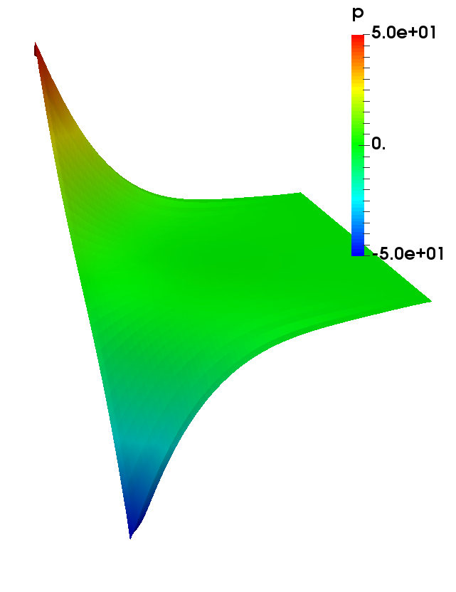
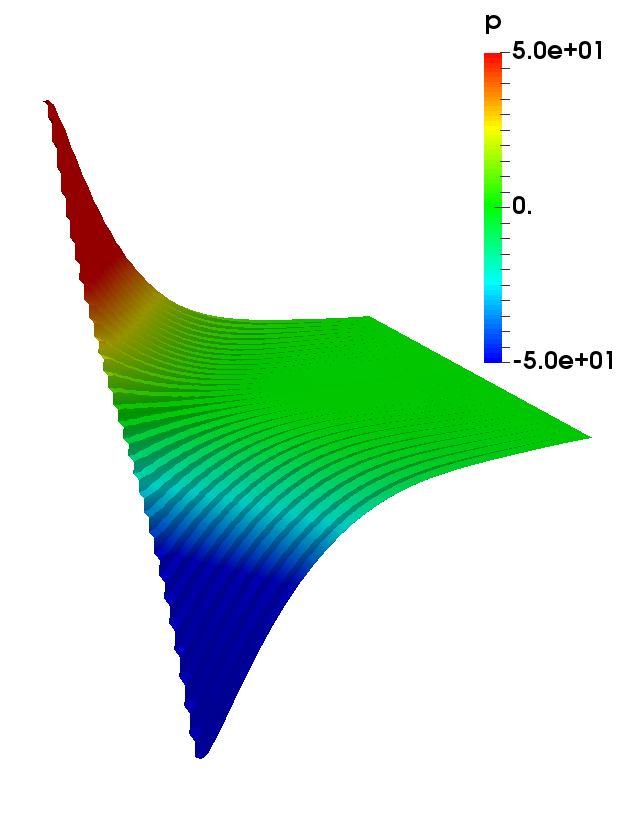
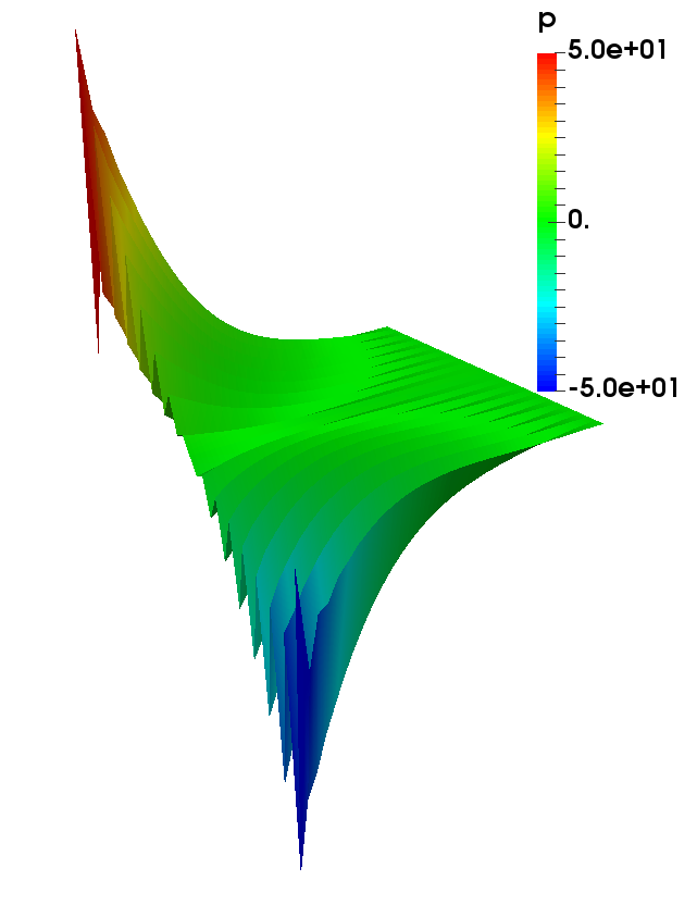
Figure 5: Visualisation of the pressure variable over $\Omega$ for the three different stabilisations $S,S_{2}$ and $S_{cip}$ (from left to right) on the mesh with $H=1/16$.

In Table 1, we show the $L^{2}$ and $H^{1}$-norm errors of the velocities and of pressure on four different meshes. The stabilisation parameter has been chosen $\gamma=10^{-2}$ for $S$ and by a factor of $4$ larger for $S_{2}$ and $S_{cip}$, as on regular cells we have $h_{n}\approx h_{\tau}\approx H/2$. The velocity norm errors do not show significant differences for the different stabilisations. Therefore we show only the values for the anisotropic stabilisation $S$. The convergence rates for the velocities are as expected.

Concerning the pressure approximation the situation is different. We observe only slow convergence for the standard CIP stabilisation $S_{cip}$ in the $L^{2}$-norm of pressure, especially on the finer meshes. Changing the weights from $h_{\tau}$ to $h_{n}$ or $H$ or choosing a larger parameter for $\gamma$ did not lead to considerable improvements.

The anisotropic stabilisations, on the other hand, seem to converge even faster than linearly, which would be expected from the analysis, as the averages are used everywhere ($\Omega_{h}^{\text{aniso}}=\Omega$). On the finer meshes, we see a clear advantage of the weighting used in the analysis ($S$) compared to using local cell sizes ($S_{2}$). For this weighting we observe even convergence in the $H^{1}$-seminorm error of the pressure, which increases for $S_{2}$ and $S_{cip}$.

The reason for the different convergence behaviours becomes clear, when we plot the pressure solution over $\Omega$ for the three stabilisations, see Figure 5 for $H=1/16$. For $S_{cip}$ we observe wild oscillations, which shows that the standard interior penalty stabilisation is not suitable to control the pressure on this anisotropic mesh. Smaller oscillations are visible for the term $S_{2}$, that are due to to wrong scaling of the derivatives. The stabilisation $S$ leads in contrast to a smooth behaviour of $p$.

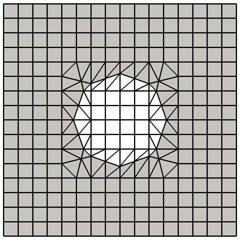
Figure 6: Illustration of the coarsest mesh used for the numerical example of Section 6.2 for $x_{0}=0$. The domain $\Omega_{h,f}$ is visualised in grey.

6.2 Example 2: Different kind of anisotropies within the locally modified finite element method

Next, we show that the proposed pressure stabilisation can be used in combination with the locally modified finite element method to approximate curved boundaries with all kinds of arising anisotropies.

To define the geometry we extract an inner circle of radius $r=0.4$: $\Omega=(-1,1)^{2}\setminus B_{0.4}(x_{0},y_{0})$ from the unit square. The boundary $\partial\Omega$ is a mixture of a polygon and a smooth boundary, such that the theoretical results hold true (cf. Remark 5.5). We discretise the unit square with a uniform patch mesh and resolve the circular boundary by means of the locally modified finite element method. We define the set ${\cal T}_{h}^{\text{aniso}}$ as the union of all patches that are cut by the circle. A sketch of a coarse mesh for $(x_{0},y_{0})=(0,0)$ is given in Figure 6. While this mesh is quite isotropic, strong anisotropies will arise when we change the horizontal position $x_{0}$ of the midpoint of the circle. We use again the manufactured solution (37) and the data and boundary conditions specified in the previous example. Additionally, we impose homogeneous Dirichlet conditions on the boundary of the circle.

First, we consider the case that the midpoint of the circle coincides with the origin $x_{0}=y_{0}=0$. For ease of implementation, we extend $v$ by zero in the inner circle and use a harmonic extension of the pressure there. We use the stabilisation $S$ defined and analysed in this work. As in the previous example, we define a second stabilisation $S_{2}$ that uses the local cell sizes $h_{n}$ and $h_{\tau}$ as weights instead of $H$. Precisely, we define

$$\begin{aligned} S_{2}(p_{h},\psi_{h}):=&\gamma_{i}\sum_{e\in{\cal E}_{h}^{\text{aniso}}}\int_{e}\big{\{}h_{n}(h_{n}^{2}\partial_{n}p_{h}\partial_{n}\psi_{h}+h_{\tau}^{2}\partial_{\tau}p_{h}\partial_{\tau}\psi_{h})\big{\}}_{e}\,do\\ &+\,\gamma_{0}\sum_{e\in{\cal E}_{h}^{0}}\int_{e}\left\{h_{n}\right\}_{e}^{3}[\nabla p_{h}]_{e}\cdot[\nabla\psi_{h}]_{e}\,do.\end{aligned}$$ (38)

Note that for the regular edges in ${\cal E}_{h}^{0}$, it holds $h_{n}\sim H$ and furthermore, the jump of the tangential derivatives vanishes. As discussed in Remark 4.2, we are not able to show stability for this stabilisation on the unstructured anisotropic mesh arising from the locally modified finite element method.

Finally, we remark that in our implementation, we neglect the jump terms over outer patch edges, as they would introduce additional couplings in the system matrix. This is not the case for the mean value terms, which have to be considered on all edges $e\in{\cal E}_{h}^{\text{aniso}}$.

	$\|\nabla v-v_{h}\|_{L^{2}}$		$10^{2}\cdot\|v-v_{h}\|_{L^{2}}$		$\|p-p_{h}\|_{L^{2}}$
$H$	$S$	$S_{2}$	$S$	$S_{2}$	$S$	$S_{2}$
$1/4\;$	$18.05$	$18.04$	$74.7$	$74.5$	$3.33$	$2.82$
$1/8\;$	$9.06$	$9.06$	$18.7$	$18.6$	$1.09$	$0.91$
$1/16$	$4.52$	$4.52$	$4.67$	$4.67$	$0.36$	$0.29$
$1/32$	$2.26$	$2.26$	$1.17$	$1.17$	$0.12$	$0.10$
Estim.	0.99	0.99	1.99	1.99	1.60	1.63
Expect.	1.00		2.00		1.00

Table 2: $L^{2}$- and $H^{1}$-norm of the velocity and $L^{2}$-norm error of the pressure for two different stabilisation variants. We estimated the convergence order by a least squares fit of the function $e(h)=ch^{\alpha}$ and show the expected convergence rates from Theorem 5.1.

In Table 2, we show the $L^{2}$- and the $H^{1}$-norm error of the velocity as well as the $L^{2}$-norm error of the pressure for the two stabilisations on four different meshes. Furthermore, we show an estimated convergence order based on the calculations. The stabilisation parameter is chosen $\gamma_{i}=\gamma_{0}=2.5\cdot 10^{-3}$ for $S$ and again by a factor of 4 larger for $S_{2}$.

While the velocity errors are almost identical for both stabilisations, the pressure error is slightly smaller for $S_{2}$. The convergence behaviour of the velocity norms coincides almost perfectly with the theoretical results for $S$ given above. The $L^{2}-$norm of the pressure converges with a higher order $\alpha\geq 1.5$ for both stabilisations, while we had only shown first order convergence in Theorem 5.1. This can be explained by means of super-convergence effects due the structured grid in the sub-domain $\Omega_{h}^{0}$. The errors seen here are essentially a combination of interpolation errors and the error contribution from the non-consistency of the stabilisation term in $\Omega_{h}^{\text{aniso}}$. For the $L^{2}$-norm of the pressure, the latter is dominant and restricts the convergence order to ${\cal O}(H^{3/2})$.

In order to study the effect of different anisotropies, we move the midpoint of the circle next in intervals of $10^{-3}$ up to $x_{0}=0.249$ to the right. This covers all kinds of anisotropies, as for $x_{0}=0.25$ the midpoint moves by exactly one patch on the coarsest grid. Exemplarily we show in Figure 7 some of the most anisotropic cells that arise, with a maximum aspect ratio of $1893.9$. Moreover, we give some details of the maximum anisotropies for four different positions $x_{0}$ in Table 3.

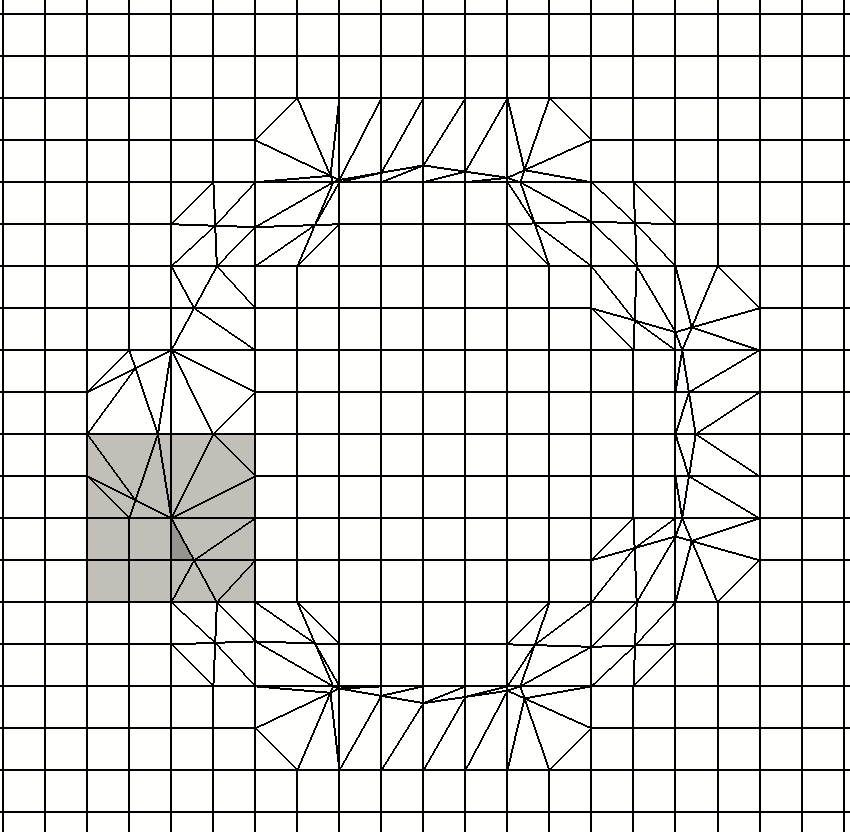
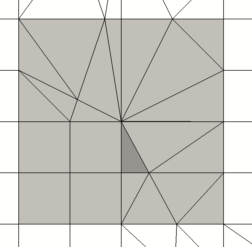
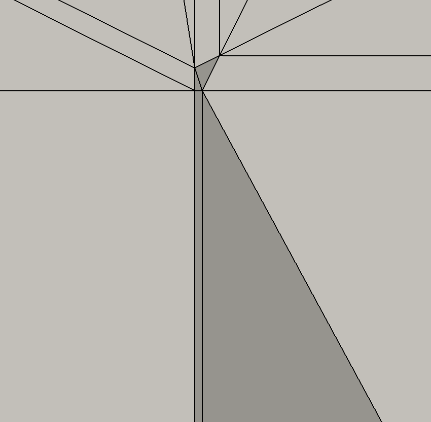
Figure 7: Visualisation of the mesh anisotropy for $H=1/8$ and $x_{0}=0.006$. From left to right, we zoom twice around the light gray and the dark gray area, respectively. The aspect ratio of the vertically stretched gray triangle that is only visible in the second zoom on the right is around $1893.9$.

$x_{0}$	$|K_{\max}|$	$|K_{\min}|$	$\frac{|K_{\max}|}{|K_{\min}|}$	$|e_{\text{max}}|$	$|e_{\text{min}}|$	$\max\limits_{K\in\mathcal{T}_{h}}\varkappa_{K}$
0	$4.99\cdot 10^{-3}$	$2.28\cdot 10^{-5}$	$2.20\cdot 10^{2}$	$1.36\cdot 10^{-1}$	$3.97\cdot 10^{-3}$	$1.58\cdot 10^{1}$
0.006	$5.85\cdot 10^{-3}$	$1.65\cdot 10^{-9}$	$3.55\cdot 10^{6}$	$1.40\cdot 10^{-1}$	$3.30\cdot 10^{-5}$	$1.89\cdot 10^{3}$
0.015	$5.84\cdot 10^{-3}$	$6.98\cdot 10^{-9}$	$8.37\cdot 10^{5}$	$1.45\cdot 10^{-1}$	$7.20\cdot 10^{-5}$	$8.85\cdot 10^{2}$
0.045	$4.93\cdot 10^{-3}$	$1.86\cdot 10^{-4}$	$2.66\cdot 10^{1}$	$1.41\cdot 10^{-1}$	$1.25\cdot 10^{-2}$	$5.12$

Table 3: Properties of the mesh $\mathcal{T}_{h}$ for $H=1/8$ for four different positions $x_{0}$. In columns 2 to 4, we show the area of the largest and the smallest element $|K_{\max}|$ and $|K_{\min}|$ and their ratio; in columns 5 and 6 the size of the largest and smallest edge $|e_{\text{max}}|$ and $|e_{\text{min}}|$. Finally, in column 7 the biggest aspect ratio $\varkappa_{K}=\frac{|e_{K,\text{max}}|}{|e_{K,\text{min}}|}$ of all elements $K\in\mathcal{T}_{h}$ is shown. For $x_{0}=0.006$ and $0.015$, two very anisotropic grids emerge, while for $x_{0}=0.045$ the grid is almost isotropic.

In Figure 8 (left sketch), we plot the $H^{1}$-norm of the pressure over $x_{0}$ for the stabilisation term $S$ and for the four different meshes. The norm increases uniformly when the circle moves to the right as the analytical solution $p$ increases. We do not observe any instabilities on any of the four grids. This shows in particular that the observed convergence behaviour for $x_{0}=0$ in Table 2 is obtained on the more anisotropic grids for $x_{0}>0$ as well.

In the right sketch, we compare the two different stabilisations on the second-coarsest mesh with $H=1/8$. Again, we do not observe any oscillations.

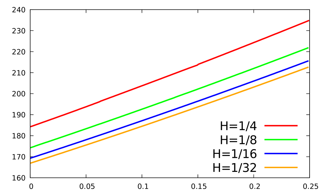
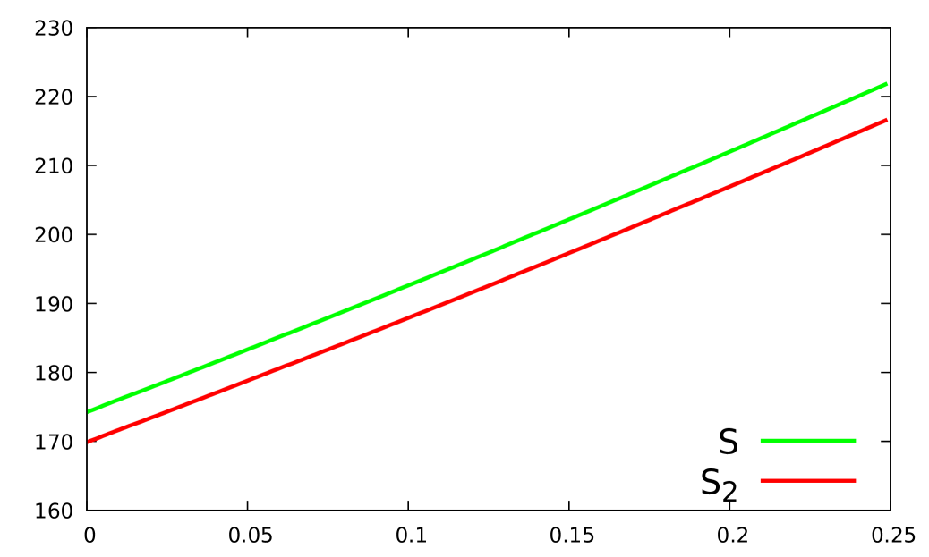
Figure 8: $H^{1}$-norm of the discrete pressure for different positions $(x_{0},0)$ of the midpoint of the circle plotted over $x_{0}$. Left: Stabilisation $S$ on different mesh levels, right: Both stabilisations for the mesh with patch size $H=0.125$.

6.3 Example 3: A non-linear fluid-structure interaction problem

To show the capabilities of the approach, we consider a non-stationary and non-linear fluid-structure interaction problem with moving interface. The overall geometry $\Omega$ is the same as in the previous example, with the difference that the inner ball is now elastic and will be both deformed and moved by the fluid forces. The sub-domains are denoted by $\Omega_{f}(t)$ and $\Omega_{s}(t)$, separated by an interface $\Gamma_{i}(t)$. We consider the incompressible Navier-Stokes equations in the fluid domain $\Omega_{f}(t)$. In the solid domain $\Omega_{s}(t)$, we impose a hyper-elastic non-linear St.Venant Kirchhoff material law. Together with the standard FSI coupling conditions, the complete set of equations for the fluid velocity $v_{f}$, the pressure $p_{f}$, the solid displacement $u_{s}$ and the solid velocity $v_{s}$ reads in Eulerian coordinates

$$\begin{split}\rho_{f}\partial_{t}v_{f}+\rho_{f}(v_{f}\cdot\nabla)v_{f}-\operatorname{div}\sigma_{f}&=\rho_{f}f\\ \operatorname{div}v_{f}&=0\;\end{split}\quad\;\Bigg{\}}\quad\text{in }\;\Omega_{f}(t),$$

$$\begin{split}J\rho^{0}_{s}(\partial_{t}v_{s}+v_{s}\cdot\nabla v_{s})-\operatorname{div}\sigma_{s}&=J\rho_{s}^{0}f\\ \partial_{t}u_{s}+v_{s}\cdot\nabla u_{s}-v_{s}&=0\end{split}\quad\Bigg{\}}\quad\text{in }\;\Omega_{s}(t),$$ (39)

$$\begin{split}v_{f}&=v_{s}\\ \sigma_{f}n&=\sigma_{s}n\;\end{split}\quad\;\,\Bigg{\}}\quad\text{on }\Gamma_{i}(t).$$

Here, $F=\nabla T=I-\nabla u_{s}$ denotes the deformation gradient, $J=\text{det }F$ its determinant and the solid and fluid Cauchy stress tensor are given by

$$\sigma_{s}=JF^{-1}\big{(}2\mu_{s}E_{s}+ \lambda_{s}\text{tr}(E_{s})\big{)}F^{-T},\quad E_{s}=\frac{1}{2}\left(F^{-T}F^{-1}-I\right),\quad\sigma_{f}=\frac{\rho_{f}\nu_{f}}{2}\left(\nabla v_{f}+\nabla v_{f}^{T}\right)-p_{f}I.$$

The boundary conditions for the fluid are a parabolic inflow profile on the left boundary, the do-nothing boundary condition on the right and homogeneous Dirichlet conditions on bottom and top. As material parameters, we use the viscosity $\nu_{f}=1$, the densities $\rho_{f}=\rho_{s}=1000$ and the solid Lamé parameters $\mu_{s}=10^{4}$ and $\lambda_{s}=4\cdot 10^{4}$. We start with zero initial data and increase the inflow profile gradually until at $t=0.1$ the profile $v^{d}(y)=1-y^{2}$ is reached.

To solve the system of equations, we use the monolithic Fully Eulerian approach introduced by  Dunne & Rannacher ²⁰. For time discretisation we use Rothe’s method in combination with a modified dG(0) time-stepping scheme ²⁴. Due to the moving interface the mesh changes from time step to time step. To conserve the incompressibility of the discrete solution, the old velocity is projected onto the new mesh by a Stokes projection after each time step, see Besier & Wollner ⁸. For space discretisation, we use the locally modified finite element method for all variables in combination with the analysed pressure stabilisation technique. A detailed derivation and analysis of the methods can be found in ²².

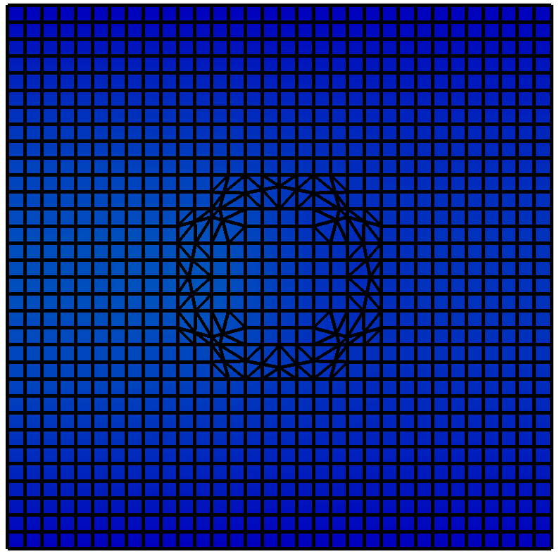
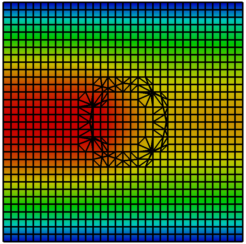
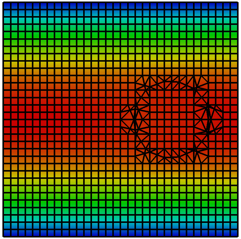
Figure 9: Snapshots of the moving ball on a coarse mesh ($H=1/8$) at times $t=0,0.1$ and $0.5$. The colouring illustrates the horizontal velocity.

We study the effect of the stabilisation terms $S$ and $S_{2}$. The stabilisation parameters are chosen $\gamma_{i}=10^{-4}$ and $\gamma_{0}=10^{-2}$ for $S$ and again by a factor of 4 larger for $S_{2}$. We use the time step $k=10^{-2}$ and patch meshes obtained by 4, 5, 6 and 7 global refinements of the unit square. For refinement level 5, the resulting mesh including the sub-triangulation that resolves the interface are shown in Figure 9 at three different instances of time. First, the ball is compressed at its left boundary ($t=0.1$, middle), then it starts to move to the right. Extremely anisotropic cells occur, as in the previous example.

In Table 4, we show the $L^{2}$-norm and the $H^{1}$-semi-norm of velocity and the $L^{2}$-norm of the pressure over the fluid domain at time $t=0.5$. Again the velocity errors are almost identical for $S$ and $S_{2}$, while we observe small deviations in the values of the pressure norm. All the values converge reasonably well, in most cases even better than predicted. Both pressure stabilisations seem to stabilise similarly well, such that in this example no clear advantage for one of the methods can be given.

	$\|\nabla v_{h}\|_{L^{2}}$		$\|v_{h}\|_{L^{2}}$		$\|p_{h}\|_{L^{2}}$
$H$	$S$	$S_{2}$	$S$	$S_{2}$	$S$	$S_{2}$
$1/4\;$	$2.320$	$2.319$	$1.354$	$1.355$	3813.1	3707.7
$1/8\;$	$2.333$	$2.333$	$1.356$	$1.356$	4608.4	4597.6
$1/16$	$2.335$	$2.335$	$1.355$	$1.355$	4832.8	4832.6
$1/32$	$2.335$	$2.335$	$1.354$	$1.354$	4912.4	4912.1

Table 4: Behaviour of velocity and pressure norms under mesh refinement for the two different stabilisation terms.

Finally, we show a plot of the pressure at time $t=0.5$ on a coarse and a fine mesh in Figure 10 for the stabilisation $S$. We see that on both meshes the pressure is nicely controlled by the stabilisation. On the coarser mesh, however, the fine scale behaviour of the pressure near the interface $\Gamma_{i}$ is significantly disturbed.

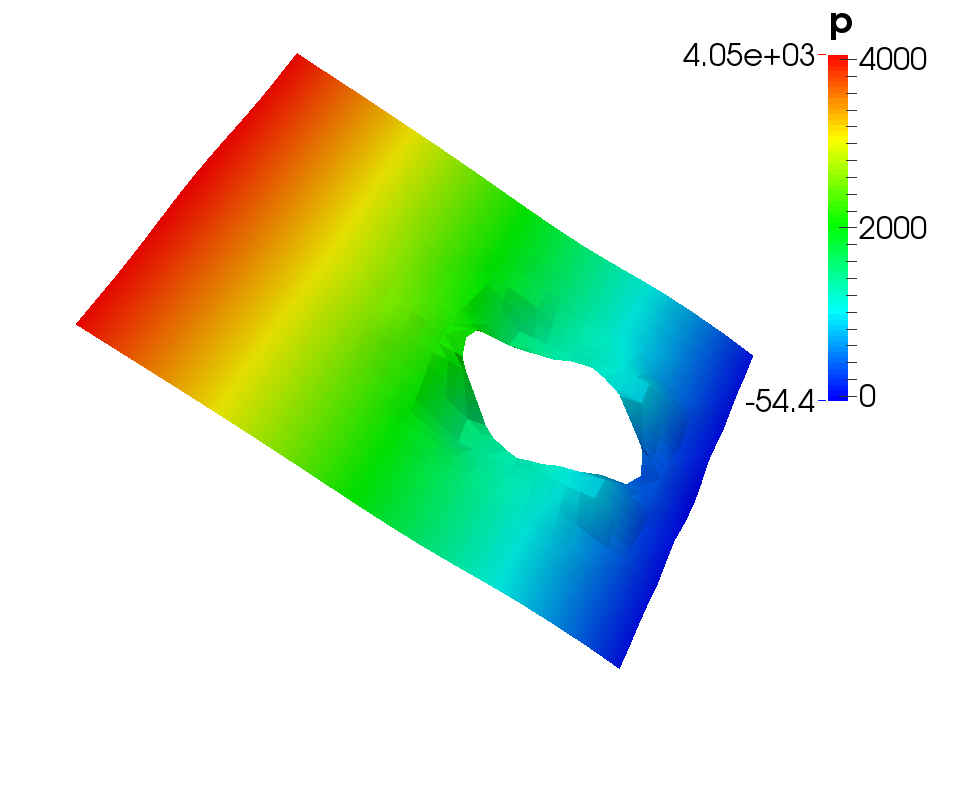
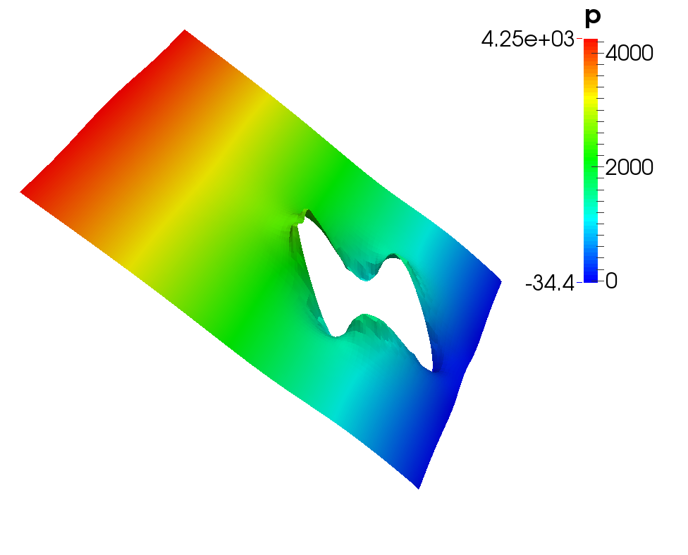
Figure 10: Pressure profiles for stabilisation $S$ at time $t=0.5$ on a coarse mesh $H=1/8$ (left) and a fine mesh $H=1/32$ (right).

7 Conclusion

We have presented a pressure stabilisation scheme that is able to deal with anisotropic grids without bounded change of anisotropy. The approach is especially suitable if only a small part of the mesh is anisotropic, which is typical for interface problems and problems with complex boundaries. Our numerical results show that in contrast to the standard interior penalty pressure stabilisation the proposed method is able to control the pressure on arbitrarily anisotropic meshes without bounded changes in anisotropy. A possible extension of this work includes the stabilisation of convection-dominated convection-diffusion problems.

Moreover, the pressure stabilisation can be extended to three space dimensions using the corresponding stabilisation term on faces instead of edges. The extension of the locally modified finite element method to three space dimensions is in principal also possible. The implementation is however subject to future work.

References

- Acosta and Durán [2000] Gabriel Acosta and Ricardo G Durán. Error estimates for Q1 isoparametric elements satisfying a weak angle condition. SIAM Journal on Numerical Analysis, 38(4):1073–1088, 2000.
- Ainsworth and Coggins [2000] Mark Ainsworth and Patrick Coggins. The stability of mixed hp-finite element methods for stokes flow on high aspect ratio elements. SIAM Journal on Numerical Analysis, 38(5):1721–1761, 2000.
- Apel [1999] Thomas Apel. Anisotropic finite elements: local estimates and applications, volume 3. 1999.
- Apel et al. [2008] Thomas Apel, Tobias Knopp, and Gert Lube. Stabilized finite element methods with anisotropic mesh refinement for the oseen problem. Applied Numerical Mathematics, 58(12):1830–1843, 2008.
- Babuška and Aziz [1976] Ivo Babuška and A Kadir Aziz. On the angle condition in the finite element method. SIAM Journal on Numerical Analysis, 13(2):214–226, 1976.
- Babuška [1970] Ivo Babuška. The finite element method for elliptic equations with discontinuous coefficients. Computing, 5:207–213, 1970.
- Becker and Braack [2001] Roland Becker and Malte Braack. A finite element pressure gradient stabilization for the Stokes equations based on local projections. Calcolo, 38(4):173–199, 2001.
- Besier and Wollner [2012] Michael Besier and Winnifried Wollner. On the pressure approximation in nonstationary incompressible flow simulations on dynamically varying spatial meshes. International Journal for Numerical Methods in Fluids, 69(6):1045–1064, 2012.
- Braack and Richter [2005] Malte Braack and Thomas Richter. Local projection stabilization for the Stokes system on anisotropic quadrilateral meshes. In Bermudez de Castro et al., editor, Enumath, pages 770–778. Springer, 2005.
- Braack et al. [2012] Malte Braack, Gert Lube, and Lars Röhe. Divergence preserving interpolation on anisotropic quadrilateral meshes. Comput. Methods Appl. Math., 12(2):123–138, 2012.
- Bramble and King [1994] James H Bramble and J Thomas King. A robust finite element method for non-homogeneous Dirichlet problems in domains with curved boundaries. Mathematics of Computation, 63:1–17, 1994.
- Burman and Hansbo [2004] Erik Burman and Peter Hansbo. Edge stabilization for Galerkin approximations of convection–diffusion–reaction problems. Computer Methods in Applied Mechanics and Engineering, 193(15):1437–1453, 2004.
- Burman and Hansbo [2006] Erik Burman and Peter Hansbo. Edge stabilization for the generalized Stokes problem: a continuous interior penalty method. Computer Methods in Applied Mechanics and Engineering, 195(19):2393–2410, 2006.
- Burman et al. [2006] Erik Burman, Miguel A Fernández, and Peter Hansbo. Continuous interior penalty finite element method for oseen’s equations. SIAM journal on numerical analysis, 44(3):1248–1274, 2006.
- Castro-Diaz et al. [1997] MJ Castro-Diaz, F Hecht, B Mohammadi, and O Pironneau. Anisotropic unstructured mesh adaption for flow simulations. International Journal for Numerical Methods in Fluids, 25(4):475–491, 1997.
- Ciarlet [1991] Philippe G Ciarlet. Basic error estimates for elliptic problems. In P.G. Ciarlet and J.L. Lions, editors, Handbook of Numerical Analysis, volume 2, pages 17–351. Elsevier, 1991.
- Ciarlet [2002] Philippe G Ciarlet. The finite element method for elliptic problems. SIAM, 2002.
- Clément [1975] Philippe Clément. Approximation by finite element functions using local regularization. RAIRO: Analyse numérique, 9:77–84, 1975.
- Codina and Soto [2004] Ramon Codina and Orlando Soto. Approximation of the incompressible navier–stokes equations using orthogonal subscale stabilization and pressure segregation on anisotropic finite element meshes. Computer Methods in Applied Mechanics and Engineering, 193(15):1403–1419, 2004.
- Dunne and Rannacher [2006] Thomas Dunne and Rolf Rannacher. Adaptive finite element approximation of fluid-structure interaction based on an Eulerian variational formulation. In H.-J. Bungartz and M. Schäfer, editors, Fluid-Structure Interaction: Modeling, Simulation, Optimization, Lecture Notes in Computational Science and Engineering, pages 110–145. Springer, 2006.
- Formaggia et al. [2004] Luca Formaggia, Stefano Micheletti, and Simona Perotto. Anisotropic mesh adaptation in computational fluid dynamics: Application to the advection-diffusion-reaction and the stokes problems. Appl. Numer. Math., 51(4):511–533, 2004. ISSN 0168-9274.
- Frei [2016] Stefan Frei. Eulerian finite element methods for interface problems and fluid-structure interactions. PhD thesis, Heidelberg University, 2016. urn:nbn:de:bsz:16-heidok-215905.
- Frei and Richter [2014] Stefan Frei and Thomas Richter. A locally modified parametric finite element method for interface problems. SIAM Journal on Numerical Analysis, 52(5):2315–2334, 2014.
- Frei and Richter [2017] Stefan Frei and Thomas Richter. A second order time-stepping scheme for parabolic interface problems with moving interfaces. ESAIM: M2AN, 51(4):1539–1560, 2017.
- Frei et al. [2015a] Stefan Frei, Thomas Richter, and Thomas Wick. Eulerian techniques for fluid-structure interactions: Part i-modeling and simulation. In Assyr Abdulle, Simone Deparis, Daniel Kressner, Fabio Nobile, and Marco Picasso, editors, Numerical Mathematics and Advanced Applications - ENUMATH 2013: Proceedings of ENUMATH 2013, pages 745–753. Springer International Publishing, 2015a.
- Frei et al. [2015b] Stefan Frei, Thomas Richter, and Thomas Wick. Eulerian techniques for fluid-structure interactions: Part ii – applications. In Assyr Abdulle, Simone Deparis, Daniel Kressner, Fabio Nobile, and Marco Picasso, editors, Numerical Mathematics and Advanced Applications - ENUMATH 2013: Proceedings of ENUMATH 2013, pages 755–762. Springer International Publishing, 2015b.
- Frei et al. [2016] Stefan Frei, Thomas Richter, and Thomas Wick. Long-term simulation of large deformation, mechano-chemical fluid-structure interactions in ale and fully eulerian coordinates. Journal of Computational Physics, 321:874 – 891, 2016.
- Gangl and Langer [2016] P. Gangl and U. Langer. A Local Mesh Modification Strategy for Interface Problems with Application to Shape and Topology Optimization. ArXiv e-prints, 2016.
- Grossmann et al. [2007] Christian Grossmann, Hans-Görg Roos, and Martin Stynes. Numerical treatment of partial differential equations, volume 154. Springer, 2007.
- Hoffman et al. [2017] Johan Hoffman, Bärbel Holm, and Thomas Richter. The locally adapted parametric finite element method for interface problems on triangular meshes. In S. Frei, B. Holm, T. Richter, T. Wick, and H. Yang, editors, Fluid-Structure Interaction: Modeling, Adaptive Discretization and Solvers, Radon Series on Computational and Applied Mathematics. Walter de Gruyter, Berlin, 2017.
- Hughes et al. [1986] Thomas JR Hughes, Leopoldo P Franca, and Marc Balestra. A new finite element formulation for computational fluid dynamics: V. circumventing the babuška-brezzi condition: a stable petrov-galerkin formulation of the stokes problem accommodating equal-order interpolations. Computer Methods in Applied Mechanics and Engineering, 59(1):85–99, 1986.
- Hughes et al. [1988] TJR Hughes, LP Franca, GM Hulbert, Z Johan, and F Shakib. The galerkin/least-squares method for advective-diffusive equations. In Recent Developments in Computational Fluid Dynamics, pages 75–99, 1988.
- John and Knobloch [2007] Volker John and Petr Knobloch. On spurious oscillations at layers diminishing (sold) methods for convection–diffusion equations: Part i–a review. Computer methods in applied mechanics and engineering, 196(17-20):2197–2215, 2007.
- Knauf et al. [2014] Stefan Knauf, Stefan Frei, Thomas Richter, and Rolf Rannacher. Towards a complete numerical description of lubricant film dynamics in ball bearings. Computational Mechanics, 53(2):239–255, 2014.
- Langer and Yang [2015] Ulrich Langer and Huidong Yang. Numerical simulation of parabolic moving and growing interface problems using small mesh deformation. arXiv preprint arXiv:1507.08784, 2015.
- Linß [2009] Torsten Linß. Layer-adapted meshes for reaction-convection-diffusion problems. Springer, 2009.
- Loseille et al. [2010] Adrien Loseille, Alain Dervieux, and Frédéric Alauzet. Fully anisotropic goal-oriented mesh adaptation for 3d steady euler equations. Journal of computational physics, 229(8):2866–2897, 2010.
- Micheletti and Perotto [2008] Stefano Micheletti and Simona Perotto. Output functional control for nonlinear equations driven by anisotropic mesh adaption: the navier–stokes equations. SIAM Journal on Scientific Computing, 30(6):2817–2854, 2008.
- Micheletti and Perotto [2011] Stefano Micheletti and Simona Perotto. The effect of anisotropic mesh adaptation on pde-constrained optimal control problems. SIAM Journal on Control and Optimization, 49(4):1793–1828, 2011.
- Micheletti et al. [2003] Stefano Micheletti, Simona Perotto, and Marco Picasso. Stabilized finite elements on anisotropic meshes: A priori error estimates for the advection-diffusion and the stokes problems. SIAM Journal on Numerical Analysis, 41(3):1131–1162, 2003.
- Pauli and Behr [2017] L. Pauli and M. Behr. On stabilized space-time fem for anisotropic meshes: Incompressible navier-stokes equations and applications to blood flow in medical devices. International Journal for Numerical Methods in Fluids, 85(3):189–209, 2017.
- Richter [2010] Thomas Richter. A posteriori error estimation and anisotropy detection with the dual-weighted residual method. International journal for numerical methods in fluids, 62(1):90–118, 2010.
- Richter [2017] Thomas Richter. Fluid-structure Interactions: Models, Analysis and Finite Elements, volume 118. Springer, 2017.
- Roos et al. [2008] Hans-Görg Roos, Martin Stynes, and Lutz Tobiska. Robust numerical methods for singularly perturbed differential equations: convection-diffusion-reaction and flow problems, volume 24. Springer Science & Business Media, 2008.
- Scott and Zhang [1990] L Ridgeway Scott and Shangyou Zhang. Finite element interpolation of nonsmooth functions satisfying boundary conditions. 54(190):483–493, 1990.
- Siebert [1996] Kunibert G. Siebert. An a posteriori error estimator for anisotropic refinement. Numerische Mathematik, 73(3):373–398, May 1996.
- Temam [2000] Roger Temam. Navier-Stokes Equations: Theory and Numerical Analysis. American Mathematical Society, 2000.