Efficient Tensor Decomposition with Boolean Factors

Abstract

Tensor decomposition has been extensively used as a tool for exploratory analysis. Motivated by neuroscience applications, we study tensor decomposition with Boolean factors. The resulting optimization problem is challenging due to the non-convex objective and the combinatorial constraints. We propose Binary Matching Pursuit (BMP), a novel generalization of the matching pursuit strategy to decompose the tensor efficiently. BMP iteratively searches for atoms in a greedy fashion. The greedy atom search step is solved efficiently via a MAXCUT-like boolean quadratic program. We prove that BMP is guaranteed to converge sublinearly to the optimal solution and recover the factors under mild identifiability conditions. Experiments demonstrate the superior performance of our method over baselines on synthetic and real datasets. We also showcase the application of BMP in quantifying neural interactions underlying high-resolution spatiotemporal ECoG recordings.

1 Introduction

Tensors, as high-order generalizations of matrices, provide concise representation for multi-way data. Tensor decomposition, with direct connections with latent variable modeling [1], has been a popular tool for exploratory analysis, e.g. [2, 3]. Most tensor decomposition methods assume all the factors are continuous-valued representing a mixture of all latent components. However, Boolean factors indicating the presence or absence of latent components are preferred in certain applications such as molecular genetics [4] and clinic medicine [5]. In neuroscience, for instance, given spatiotemporal neural activities, Boolean factors can better help us answer the “when” and “where” questions regarding the underlying brain network patterns. This motivates the study of tensor decomposition methods with Boolean factors in this paper.

The difficulty of tensor decomposition mainly stems from the fact that the set of low-rank tensors $\{\mathcal{X}|\mathcal{X}\in\mathbb{R}^{d_{1}\times d_{2}\times d_{3}},\text{rank}(\mathcal{X})\leq R\}$ is non-convex and in general not closed. As such, the Maximum Likelihood Estimator (MLE) objective is non-convex and the best rank-R approximation of a tensor may not exist [6]. This difficulty is magnified by the combinatorial constraint of Boolean factors. To bypass the MLE objective, [7, 1, 8, 9] proposed a method of moments estimator, which achieves global guarantees in the average case. However, they rely on the strong distributional assumptions on the latent factors and can be unstable in model mis-specification cases. [10, 11, 12] propose to use nuclear norm as a convex surrogate for the rank constraints, but can be computational challenging for large-scale problems.

To tackle the Boolean constraint, [13] considered the noiseless case and proposed a geometric algorithm, but their method has exponential complexity in the rank of the decomposition. [14] improved the solver using convex relaxation that achieves linear sample complexity w.r.t the rank and the dimensions. Our setting is a special case of Boolean tensor decomposition [15, 5] where the input tensor is also Boolean. [15, 5] proposed algorithms based on alternating least square (ALS) followed by rounding heuristics. However, ALS does not perform well in the presence of highly noisy measurements. [4] studied a Bayesian version of the problem and apply Monte Carlo sampling. The theoretical behavior of these methods are not well understood.

We provide an efficient solution for learning tensor decomposition with Boolean factors. Using atomic norm, we cast the non-convex tensor decomposition problem as a convex program with sparsity constraints, which enjoys tractable relaxations. We propose a novel algorithm, Boolean Matching Pursuit (BMP), to search for atoms of the steepest descent iteratively. Our algorithm enjoys strong theoretical guarantees. It can recover the parameters exactly under identifiability conditions with sublinear convergence. The sample complexity scales only linearly with the rank of the tensor. We validated the superior performance of BMP on synthetic and neural recordings. In summary, our contributions include:

• We study a novel tensor decomposition model with Boolean factors, which is particularly suitable for exploratory analysis of discretized spatiotemporal data.

• We formulate the non-convex problem as an atomic-norm regularized convex program and propose a fast algorithm Binary Matching Pursuit (BMP) to solve the problem efficiently.

• Our algorithm is guaranteed to converge sub-linearly to the optimal solution, with run-time and sample complexity only linear in the number of atoms.

• We experiment extensively on synthetic and real-world ECoG datasets and observe superior performance for denoising and completion tasks. Our algorithm also uncovers the interesting neural mechanism underlying consciousness in brain computer interface (BCI).

2 Related Work

Tensor decomposition.

Tensor decomposition has been the subject of extensive study; please see the review paper by [16] and references therein. Most tensor factorization work focuses on extracting high-order structure with continues-value factors. For instance, [17, 18] proposed orthogonalized ALS to decompose a tensor alternatively but are only limited to orthogonal factors. [19, 20, 3] developed nuclear norm regularization as a convex surrogate and solve the problem using alternating direction method of multipliers (ADMM). But can suffer from high computational costs. [2] designed a non-convex solver based on a greedy algorithm and demonstrate significant speedup. There has also been work on Boolean tensor decomposition where the input tensor has Boolean values [21, 22], which is different from our problem where the learned factors are Boolean. [15, 5] proposed algorithms based on alternating least square (ALS) with rounding heuristics. To the best of our knowledge, our work is the first algorithm for tensor decomposition with Boolean factors with theoretical guarantees.

Boolean constrained latent variable model.

Latent variable model with Boolean constraints is also known as latent feature model (LFM) [23] in statistical learning, where each observation is associated with a set of real-valued latent features and Boolean vector indicating the presence/absence of the features. For the parametric version of the model, [7, 1, 8] propose to use spectral methods to estimate the moments of the distribution at different orders, but can suffer from high sample complexity. Under certain identifiability condition, [13] proposed a convex optimization algorithm by selecting a maximal affine independent subset. However, the selection process in their algorithm has an exponential computational complexity. Perhaps the work that is most related to ours is [14] in which a convex estimator for matrix latent feature models which under certain identifiability conditions achieves a linear sample complexity. LFMs also bear affinity to sparse dictionary learning [24] whereas the representations are real-valued instead of Boolean.

Preliminary

Across the paper, we use calligraphy font for tensors, such as $\mathcal{X},\mathcal{Y}$, bold uppercase for matrices, such as $\mathbf{X},\mathbf{Y}$, and bold lowercase for vectors, such as $\boldsymbol{x},\boldsymbol{y}$. For easy of illustration, we use order-$3$ tensor throughout the paper. Our results directly generalize to high-order cases.

Mode-$n$ Unfolding: For an order-$3$ tensor $\mathcal{X}\in\mathbb{R}^{d_{1}\times d_{2}\times d_{3}}$, a mode-$n$ unfolding is to matricize a tensor along a particular mode $\mathbf{X}=\mathrm{unfold}_{n}(\mathcal{X})$ with $d_{n}$ rows and $\prod_{i}d_{i}/d_{n}$ columns. The mode-$n$ refold $\mathcal{X}=\mathrm{refold}_{n}(\mathbf{X})$ is the reverse operation. The indexing follows the convention in [16].

Tensor Rank: The rank of a tensor is the minimum number of rank-1 components it contains:
$\text{rank}_{\otimes}(\mathcal{X})=:\{\min R|\mathcal{X})=\sum_{r=1}^{R}\boldsymbol{u}_{r}\otimes\boldsymbol{v}_{r}\otimes\boldsymbol{w}_{r}\}$. Multilinear rank is a tuple $(R_{1},R_{2},R_{3})$ such that $R_{n}=\text{rank}(\text{unfold}_{n}(\mathcal{X}))$. We have $R_{n}\leq\min(\text{rank}_{\otimes}(\mathcal{X}),d_{n})$.

3 Tensor Decomposition with Boolean Factors

3.1 Boolean Canonical Polyadic Decomposition

Consider the following tensor decomposition model for an order-$N(N=3)$ tensor $\mathcal{X}\in\mathbb{R}^{d_{1}\times d_{2}\times d_{3}}$:

$$\mathcal{X}=\sum_{n=1}^{N}\sum_{r=1}^{R}\boldsymbol{z}^{r}_{n}\otimes\boldsymbol{u}^{r}_{n}\otimes\boldsymbol{w}^{r}_{n}+\mathcal{E}$$ (1)

where one of the factors is Boolean and the rest are continuous-valued. The noise tensor $\mathcal{E}$ has the same size as $\mathcal{X}$ with i.i.d Gaussian entries of zero mean and variance $\sigma^{2}$. The subscript $n$ indicates the mode with Boolean factors. The dimensions of the factors change accordingly. For instance, if the first mode factors are Boolean, $\boldsymbol{z}^{r}_{1}\in\mathbb{Z}_{2}^{d_{1}}$, $\boldsymbol{u}^{r}_{1}\in\mathbb{R}^{d_{2}}$ and $\boldsymbol{w}^{r}_{1}\in\mathbb{R}^{d_{3}}$.

The tensor decomposition model in (1) generalizes the latent feature model [23] to high-order tensors. Continues-valued factors represent latent features at every mode and Boolean factors indicate the presence/absence of these features. It resembles latent mixture model [20] which models a tensor as a mixture of latent tensors across modes. Latent mixture model assumes all terms to be continuous-valued, whereas our model contains Boolean factors. We name the model (1) Boolean Canonical Polyadic Decomposition.

3.2 Atomic Norm Regularized Convex Program

The estimation problem of the model in (1) is generally intractable due to non-convex optimization objective and combinatorial Boolean constraints. To make the learning tractable, we note that a tensor can be expressed as a linear combination of rank-1 tensors, or atoms. Define a mode-$n$ atomic set as $\mathds{A}_{n}:=\{\mathcal{M}|\mathcal{M}=\boldsymbol{z}^{r}_{n}\otimes\boldsymbol{u}^{r}_{n}\otimes\boldsymbol{w}^{r}_{n}\}$. The union set $\mathds{A}=\bigcup_{n}\mathds{A}_{n}$ contains all the rank-1 tensor with arbitrary Boolean factors, whose size is $\bar{K}\leq 3R$. Then the tensor decomposition problem in  (1) can be reformulated as a sparsity constrained convex program, which enjoys tractable relaxations. In particular, given an observation $\mathcal{X}\in\mathbb{R}^{d_{1}\times d_{2}\times d_{3}}$, we would like to find a sparse representation of $\mathcal{X}$ in the subspace of atoms $\mathds{A}$. We can write down the tensor decomposition problem over the atom set:

$$\min_{\boldsymbol{c},\mathcal{W}} \quad F(\mathcal{W}):=\frac{1}{2}\|\mathcal{X}-\mathcal{W}\|_{F}^{2}\quad\quad\mathrm{s.t.}\quad\mathcal{W}=\sum_{\mathcal{M}_{k}\in\mathds{A}}\boldsymbol{c}_{k}\mathcal{M}_{k},\ \|\boldsymbol{c}\|_{0}\leq\bar{K}$$ (2)

where $\|\mathcal{W}\|_{F}=\sqrt{\sum_{i_{1},\dotsc,i_{L}}\mathcal{W}_{i_{1},\dotsc,i_{L}}^{2}}$ is the tensor Frobenius norm, and $\boldsymbol{c}$ is a vector of coefficients.

The non-convexity of $\ell_{0}$ norm as well as the large number of atoms in $\mathds{A}$ make the problem in  (2) difficult. We can use the $\ell_{1}$ relaxation as a convex surrogate to $\ell_{0}$ norm, we can then utilize the notion of an atomic norm [25] as a key technical device to remedy this problem, which leads to the following tractable formulation given the atomic norm of a tensor $\mathcal{W}$:

$$\min_{\mathcal{W}}\ F(\mathcal{W})+\|\mathcal{W}\|_{\mathds{A}},\quad\|\mathcal{W}\|_{\mathds{A}}=\big{\{}\inf\ \|\boldsymbol{c}\|_{1}:\mathcal{W}=\sum_{\mathcal{M}_{k}\in\mathds{A}}\boldsymbol{c}_{k}\mathcal{M}_{k},\mathcal{M}=\boldsymbol{z}^{r}_{n}\otimes\boldsymbol{u}^{r}_{n}\otimes\boldsymbol{w}^{r}_{n}\big{\}}$$ (3)

which is a convex program with an atomic norm regularizer defined over the subspace of rank-1 tensors. The atomic norm regularized problem (3) is still difficult as the size of the atomic set grows exponentially with the order of the tensor. To avoid exhaustive search in the atomic set, we develop a fast and easy to implement optimization algorithm based on matching pursuit.

3.3 Background in Matching Pursuit

Matching pursuit (MP)  [26, 27] is a sparse approximation procedure that aims to find the “best match” of the data onto a set of atoms. Matching pursuit was initially developed for the continuous-valued vector inputs. Specifically, given an input vector $\boldsymbol{x}\in\mathbb{R}^{d}$, MP approximates $\boldsymbol{x}$ using a linear combination of atoms $\boldsymbol{x}\approx\sum_{k}\boldsymbol{c}_{k}\boldsymbol{m}_{k},\boldsymbol{m}_{k}\in\mathbb{R}^{d}$. At each iteration, MP greedily searches for the atom $\boldsymbol{m}_{k}$ that maximizes the inner product with the residual and update the weights $\boldsymbol{c}$ either incrementally (greedy MP) or fully (orthogonal MP). In this paper, we generalize matching pursuit to solve tensor decomposition problems with Boolean constraints. The main difficulty of the generalization is the greedy atom search in the set of atoms, as each atom in our setting is a rank-1 tensor with a mixture of Boolean and continuous-valued components.

Algorithm 1 BooleanMatchingPursuit

1:  Input: Tensor $\mathcal{X}$

2:  Output: Tensor $\mathcal{W}$

3:  Initialize $\mathcal{W}^{0}\leftarrow 0$ , an active set $\mathds{A}\leftarrow\emptyset$

4:  for $k=0,\dotsc,K-1$ do

5:     $\mathcal{M}_{k}\leftarrow\mathrm{\texttt{GreedyAtomSearch}}(\mathcal{X},\mathcal{W}^{k})$

6:     Add to the active set $\mathds{A}\leftarrow\mathds{A}\cup\{\mathcal{M}_{k}\}$

7:     Adjust coefficients $\boldsymbol{c}$ by solving (9)

8:     Reconstruct $\mathcal{W}^{k+1}\leftarrow\sum_{\mathcal{M}_{k}\in\mathds{A}}\boldsymbol{c}_{k}\mathcal{M}_{k}$

9:  end for

Algorithm 2 GreedyAtomSearch

1:  Input: Tensor $\mathcal{X},\mathcal{W}$

2:  Output: Rank-1 tensor $\mathcal{M}$

3:  for each mode $n=1\,\dots,N$ do

4:     Gradient $G\leftarrow\mathrm{unfold}_{n}(\nabla F(\mathcal{W}))$

5:     Quadratic term $C\leftarrow-GG^{T}$

6:     Solve MAXCUT $\boldsymbol{z}\leftarrow\mathrm{\texttt{MaxCut}}(C)$

7:     Unit vector $\boldsymbol{v}\propto G^{T}\boldsymbol{z}$

8:     Candidate atom $\mathcal{M}_{n}\leftarrow\text{refold}(\boldsymbol{z}_{n}\otimes\boldsymbol{v})$

9:  end for

10:  $\mathcal{M}\leftarrow\operatorname*{arg\,min}_{\mathcal{M}_{n}}\ \big{\langle}\nabla F(\mathcal{W}),\mathcal{M}_{n}\big{\rangle}$.

4 Boolean Matching Pursuit (BMP)

We introduce Boolean Matching Pursuit (BMP), a generalization of orthogonal matching pursuit algorithm to Boolean tensors. We exploit the structure of the Boolean constraint and propose an efficient MAXCUT-like Boolean quadratic solver to greedily search for the atoms.

The high level mechanism of our proposed BMP algorithm is the same as MP. As detailed in Algorithm 1, we maintain an active set of atoms $\mathds{A}$ for the selected atoms. The solution is approximated by a weighted combination of atoms $\mathcal{W}=\sum_{\mathcal{M}_{k}\in\mathds{A}}\boldsymbol{c}_{k}\mathcal{M}_{k}$ iteratively. Every time, the subroutine greedily selects an atom, add this atom to the active set, followed by a full adjustment of weights to minimize the approximation error.

4.1 Greedy Atom Search

We propose an efficient search procedure for atoms with Boolean factors. At iteration $k$, we greedily search for a rank-1 tensor $\mathcal{M}=\boldsymbol{z}_{n}\otimes\boldsymbol{u}_{n}\otimes\boldsymbol{w}_{n}$ that corresponds to the steepest descent (also maximum inner product) direction in the atom set across all modes.

$$\min_{n}\min_{\mathcal{M}\in\mathds{A}_{n}}\ \big{\langle}\nabla F(\mathcal{W}^{k}),\mathcal{M}\big{\rangle}.$$ (4)

Our algorithm is “greedy” both across the modes and within each model of the unfolded tensor. A key algorithmic contribution of this work is a novel solution based on a MAXCUT like Boolean quadratic program to optimize the inner minimization problem efficiently.

Without loss of generality, assume the inner minimization solves for mode-1, we can unfold $\nabla F(\mathcal{W})$ into a $d_{1}\times d_{2}d_{3}$ matrix. Then the minimization problem in  (4) can be written as

$$\min_{\boldsymbol{z}\in\mathbb{Z}_{2}^{d_{1}},\boldsymbol{v}\in\mathbb{R}^{d_{2}d_{3}}}\ \big{\langle}\text{unfold}_{1}(\nabla F(\mathcal{W}^{k})),\boldsymbol{z}\boldsymbol{v}^{T}\big{\rangle}.$$ (5)

Where the vector $\boldsymbol{v}=\text{vec}(\boldsymbol{u}\otimes\boldsymbol{w})$ is normalized and lies in the space of continuous-valued unit vectors, when fixing $\boldsymbol{z}$ and minimizing w.r.t. $\boldsymbol{v}$, we have

$$\boldsymbol{v}^{*}(\boldsymbol{z})=\frac{\text{unfold}_{1}(\nabla F(\mathcal{W}^{k}))^{T}\boldsymbol{z}}{\|\text{unfold}_{1}(\nabla F(\mathcal{W}^{k}))^{T}\boldsymbol{z}\|}$$

Therefore, the joint minimization problem w.r.t. $(\boldsymbol{z},\boldsymbol{v})$ is equivalent to finding $\boldsymbol{z}^{*}$ such that

$$\boldsymbol{z}^{*}=\operatorname*{arg\,min}_{\boldsymbol{z}\in\mathbb{Z}_{2}^{d_{1}}}\ \boldsymbol{z}^{T}\underbrace{\nabla F(\mathcal{W}^{k})\nabla F(\mathcal{W}^{k})^{T}}_{-C}\boldsymbol{z} =\operatorname*{arg\,max}_{\boldsymbol{z}\in\mathbb{Z}_{2}^{d_{1}}}\ \boldsymbol{z}^{T}C\boldsymbol{z}.$$ (6)

which can be solved using a Boolean quadratic solver efficiently.

4.2 Boolean Quadratic Program

With change of variables, the problem in Eqn (6) is a MAXCUT-like problem, which enjoys constant approximation guarantees [14]. Specifically, define a vector $\boldsymbol{y}=2\boldsymbol{z}-1$, then $\boldsymbol{y}\in\{-1,1\}^{d_{1}}$. Augmented with a dummy variable $y_{0}\in\{-1,1\}$, the problem can be rewritten as

$$\max_{[y_{0};\boldsymbol{y}]\in\{-1,1\}^{d_{1}+1}}\ \frac{1}{4}\begin{bmatrix}y_{0}\\ \boldsymbol{y}\end{bmatrix}^{T}\underbrace{\begin{bmatrix}\boldsymbol{1}^{T}C\boldsymbol{1}&\boldsymbol{1}^{T}C\\ C\boldsymbol{1}&C\end{bmatrix}}_{\widetilde{C}}\begin{bmatrix}y_{0}\\ \boldsymbol{y}\end{bmatrix},$$ (7)

which is now in a MAXCUT-like formulation. In general, even if the quadratic factor is positive definite, i.e., $\widetilde{C}\succ 0$, the decision version of the problem is still NP-complete [28]. However, there exist semidefinite programming (SDP) relaxations that has constant factor approximation guarantees for the following problem:

$$\max_{Y\succeq 0} \quad\big{\langle}\widetilde{C},Y\big{\rangle}\quad\mathrm{s.t.}\quad\mathrm{diag}(Y)=\boldsymbol{1},$$ (8)

Rounding of the solution to the above SDP problem guarantees a $3/5$-approximation [29].

Indeed, although the polynomial time complexity of SDPs is already a big saving compared to NP-completeness, it is still impractical to employ a general SDP solver as the subroutine. Fortunately, unlike general SDPs, the SDP of the form (8) has specialized solver  [30], whose time complexity only depends linearly on the number of non-zeros in $\widetilde{C}$. This subroutine is described in Algorithm 2.

With an updated set of atoms $\mathds{A}$, we can adjust the atom weights to reflect changes in the atom set. Fixing the active set, the weight adjustment is a simple least-square problem in terms of $\boldsymbol{c}$ as:

$$\min_{\boldsymbol{c}\in\mathbb{R}^{|\mathds{A}|}} \quad\frac{1}{2}\|\mathcal{X}-\sum_{\mathcal{M}_{k}\in\mathds{A}}\boldsymbol{c}_{k}\mathcal{M}_{k}\|_{F}^{2},$$ (9)

with a closed-form solution: $\boldsymbol{c}=(\mathbf{M}^{t}op\mathbf{M})^{-1}\mathbf{M}^{\top}\mathrm{vec}(\mathcal{X})$ where $\mathbf{M}$ is a matrix of size $d_{1}d_{2}d_{3}\times\bar{K}$, each column of which is a flattened atom $\mathrm{vec}(\mathcal{M})$ in the active set.

5 Theoretical Analysis

5.1 Convergence Analysis

An important property of the Algorithm 1 is that the number of atoms comprising the output tensor $\mathcal{W}^{K}$ is equal to the number of iterations $K$, which leads to a trade-off between optimization error and computation. Assume the optimal solution $\mathcal{W}^{*}\in\mathds{A}$ has $\bar{K}$ number of atoms. By running BMP for $\Omega(\bar{K}/\epsilon)$ iterations, one can achieve a sublinear convergence to the optimal solution.

Theorem 1.

Let $\mathcal{W}^{*}$ be the optimal solution of the problem (3), and $\{\mathcal{W}^{k}\}_{k=1}^{K}$ be the sequence of iterates produced by the BMP Algorithm 1. Assume the loss function $F$ is $\beta$-smooth, then

$$F(\mathcal{W}^{k})-F(\mathcal{W}^{*})\leq\frac{2\beta\|\mathcal{W}^{*}\|_{\mathds{A}}^{2}}{\mu^{2}}\left(\frac{1}{k}\right).$$ (10)

for any $k\in[K]$ and $\mu$ is the approximation ratio for the SDP solver.

Remark: A key ingredient of our analysis is the $\mu=3/5$ constant-approximation guarantee in the greedy step given by the SDP-based MAXCUT solver, where we utilize the following guarantee for the atom $\mathcal{M}^{*}$ picked by Algorithm 2:

$$\langle\nabla F(\mathcal{W}),\mathcal{M}^{*}\rangle\leq\mu\left(\min_{\mathcal{M}\in\mathds{A}}\;\langle\nabla F(\mathcal{W}),\mathcal{M}\rangle\right).$$ (11)

Theorem 1 only establishes an error bound relative to the atomic norm of the optimal solution $\|\mathcal{W}^{*}\|_{\mathds{A}}$. If the loss function $F$ is $\gamma$-strongly convex w.r.t the support set, we have the following additional result that bounds the optimization error directly in the ratio of number of atoms $\bar{K}/K$:

Theorem 2.

Assume the loss function $F$ is $\gamma$-strongly convex w.r.t. the support set. After running $K$ iterations of the BMP Algorithm 1, the solution $\mathcal{W}^{K}$ satisfies

$$F(\mathcal{W}^{K})-F(\mathcal{W}^{*})\leq\frac{2\beta\|\mathcal{X}\|_{F}^{2}}{\gamma\mu^{2}}\left(\frac{\bar{K}}{K}\right)$$ (12)

which shows linear scaling in terms of the ratio of number of atoms $O(\frac{\bar{K}}{K})$, demonstrating the trade-off between the sparsity of the problem and the computation complexity.

5.2 Identifiability and Parameter Recovery

Identifiability is of great importance to applications, where one might be interested in interpreting the latent factors. We provide the conditions for single latent tensor where the results directly apply to the mixture model in (1). A tensor decomposition $\mathcal{W}=\sum_{r=1}^{R}\boldsymbol{z}_{r}\otimes\boldsymbol{u}_{r}\otimes\boldsymbol{w}_{r}$ is unique if for any other decomposition, $\mathcal{W}=\sum_{r=1}^{R}\boldsymbol{z}_{r}^{\prime}\otimes\boldsymbol{u}_{r}^{\prime}\otimes\boldsymbol{w}_{r}^{\prime}$, there exists a permutation $\sigma$ such that

$$\boldsymbol{z}_{r}\otimes\boldsymbol{u}_{r}\otimes\boldsymbol{w}_{r}=\boldsymbol{z}_{\sigma(r)}^{\prime}\otimes\boldsymbol{u}_{\sigma(r)}^{\prime}\otimes\boldsymbol{w}_{\sigma(r)}^{\prime}$$

When tensor $\mathcal{W}$ has a unique decomposition, the set of factors $\boldsymbol{z}$ , $\boldsymbol{u}$ and $\boldsymbol{w}$ are identifiable, up to scalars. Let $\mathbf{Z}$ be the matrix containing $\boldsymbol{z}_{r}$ as its columns. Similarly for matrices $\mathbf{U}$ and $\mathbf{W}$. The following Kruskal’s condition [31] guarantees the uniqueness of generic tensor decomposition:

Condition 1 (Kruskal).

An order-3 rank-R tensor of dimension $d_{1}\times d_{2}\times d_{3}$ is unique if

$$R\leq\frac{1}{2}\left(\text{krank}(\mathbf{Z})+\text{krank}(\mathbf{U})+\text{krank}(\mathbf{W})-2\right)$$

where $\text{krank}(\cdot)$ is the largest value of a matrix such that every subset of columns of the matrix is linearly independent. It is also easy to see that $\text{krank}(\mathbf{Z})\leq\text{rank}(\mathbf{Z})$ for any $\mathbf{Z}$. To guarantee uniqueness of the Boolean factors $\mathbf{Z}$, we need additional conditions on its column vectors.

Condition 2 (Rigidity).

The tensor decomposition problem has unique Boolean factors if any non-trivial combinations of the column vectors $\{\boldsymbol{z}_{r}\}$ would lead to a non-Boolean vector:

$$\forall\boldsymbol{c}\neq\boldsymbol{0},\quad\boldsymbol{c}^{\top}\boldsymbol{Z}\in\mathbb{Z}_{2}\iff\boldsymbol{c}\in\{\boldsymbol{e}_{i}\}$$

which means the linear subspace of $\boldsymbol{Z}$ does not contain any other Boolean vectors that are not already in $\mathbf{Z}^{n}$. This identifiability condition is in nature similar to [13]. The following theorem guarantees the exact recovery of the latent factors from tensor decomposition.

Theorem 3 (Exact Recovery).

Let $\mathcal{X}\in\mathbb{R}^{d_{1}\times d_{2}\times d_{3}}$ be a tensor $\mathcal{X}=\sum_{r=1}^{R}\boldsymbol{z}^{r}\otimes\boldsymbol{u}^{r}\otimes\boldsymbol{w}^{r}$. Under the identifiability conditions, the algorithm can recover the atom parameters $\{\boldsymbol{z}^{r},\boldsymbol{u}^{r},\boldsymbol{w}^{r}\}$ exactly.

Note that the above results are stronger than matrix case as matrix factors are not uniquely defined due to invariance under rotations. The guarantee is deterministic for the noiseless setting.

We also analyze the statistical performance of the estimator for Problem (3). Using the notion of restricted strongly convexity [32], the following theorem guarantees the sample complexity under the Gaussian noise, in which we leverage the properties of the atomic norm.

Theorem 4 (Sample Complexity).

Assume the true model $\mathcal{W}^{*}\in\mathds{A}$, and the loss function satisfies the restricted strongly convex condition. There exists a universal constant $c_{1}$ such that if we choose the regularization parameter $\lambda_{S}=\sigma\sqrt{\frac{d_{1}+d_{2}+d_{3}}{S}}$, the statistical estimator $\hat{\mathcal{W}}$ satisfies:

$$\|\hat{\mathcal{W}}-\mathcal{W}^{*}\|_{F}^{2}\leq\big{(}O_{p}\big{(}c_{1}\frac{\sigma^{2}R(d_{1}+d_{2}+d_{3})}{S}\big{)}$$

where $S$ is the number of samples and $\sigma^{2}$ is the noise variance.

Computational Complexity   Our algorithm BMP is efficient and easy to implement. Assuming $d_{1}\geq d_{2}\geq d_{3}$, the greedy atom search step involves solving continuous-valued factors in $\mathcal{O}(d_{2}d_{3})$ and an efficient Boolean quadratic program whose complexity is $\mathcal{O}(d_{1}^{2})$ at each mode. At $k$-th iteration, the least square step can be solved in $\mathcal{O}(kd_{1}d_{2}d_{3})$ if we maintain a QR decomposition of $\mathbf{M}$, though faster solution is possible if $\mathbf{M}$ is highly structured [33].

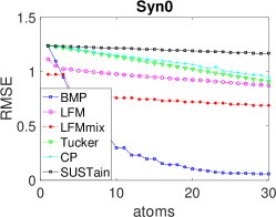
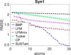
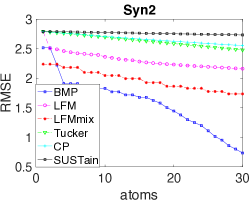
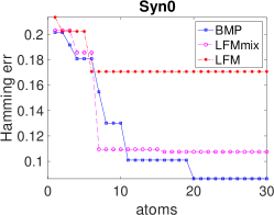
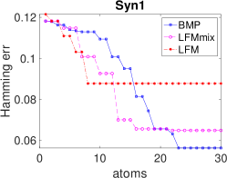
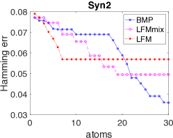
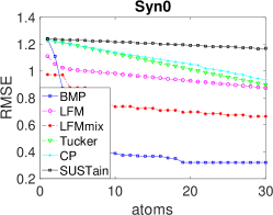
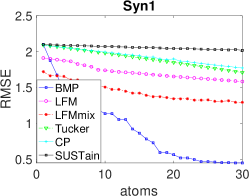
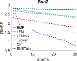
Figure 1: Performance comparison w.r.t number of atoms on synthetic datasets. Top: denoising RMSE between the ground truth and the estimated tensor. Middle: Hamming-error of the recovered Boolean factors. Bottom: completion RMSE between the ground truth and the estimated tensor.

6 Experiments

The evaluate the performance of our algorithm, we experiment with two benchmark tensor decomposition tests: denoising and completion. We compare our method with the following baselines:

• LFM [14]: matrix factorization with Boolean constraints, solved for every mode separately. Results are reported from the best mode.

• LFMmix: a mixture of latent feature matrix factors from LFM.

• Tucker: Tucker tensor decomposition solved with Higher Order SVD [34].

• CP: canonical polyadic tensor decomposition solved with ALS.

• SUSTain [5]: hierarchical ALS tensor decomposition with Boolean projection.

6.1 Synthetic Experiments

We randomly generate tensors according to model (1) of size $(150\times 150\times 150)$. For every atom $r\in[\bar{K}]$ and mode $n$, we generate a binary vector $\boldsymbol{z}^{r}_{n}\in\mathbb{Z}_{2}^{d_{n}}$ from a binomial distribution with probability $0.5$, and vectors $\boldsymbol{u}^{r}_{n},\boldsymbol{w}_{n}^{r}$ from Gaussian. We vary the number of atoms: $\bar{K}\in\{3,9,15\}$, and produce three synthetic datasets Syn0, Syn1, and Syn2.

Tensor denoising aims to estimate the tensor $\mathcal{W}$ from observations $\mathcal{X}$ contaminated by additive Gaussian noise. We synthesize the noise $\mathcal{E}\sim\mathcal{N}(0,\boldsymbol{1})$ and evaluate the root-mean-square error (RMSE) between the ground truth tensor $\mathcal{W}$ and the estimate $\hat{\mathcal{W}}$. Figure  1 top row shows the RMSE comparison of different methods w.r.t number of atoms. BMP significantly outperforms the baselines. We also observe sublinear convergence rate as predicted by Theorem 1.

To validate parameter recovery, we compare the Hamming distance between the estimated Boolean factors $\{\boldsymbol{z}^{r}_{n}\}$ and the ground truth, as shown in Figure 1 middle row. We can see that matrix-based methods LFM and LFMmix get stuck easily, and the recovery error stops decreasing after 10 atoms. In contrast, BMP can successfully recover most of the Boolean factors. Under noise, it is generally not possible to recover all the Boolean factors.

For tensor completion, a tensor $\mathcal{X}$ has missing values and the task is to complete the missing entries solely based on observations. We consider noiseless completion and randomly remove $10$ percent of the entries from the ground truth tensor $\mathcal{X}$. Figure 1 bottom row shows the RMSE between the ground truth $\mathcal{X}$ and the completed tensor $\hat{\mathcal{W}}$ from decomposition. We can see that BMP achieves the lowest completion error with only a few numbers of atoms. On the other hand, SUSTain performs poorly as the rounding step slows down the convergence.

6.2 Decoding Consciousness: Study on Brain Computer Interface

We study the neural mechanism underlying consciousness using large-scale neural activity data recorded via ECoG at high temporal (>1 KHz) and spatial (3 mm) resolution [35] with $128$ electrodes. The data were recorded from the lateral cortex in macaques during rest, anesthetic and recovery conditions. We form the data into a tensor of (space $\times$ time $\times$ trial). Boolean factors indicate whether certain latent features appear at certain spatial locations, temporal positions or trials. We split the spatiotemporal ECoG recordings into 100 bins to simulate trials. Each bin contains measurements over 3000 milliseconds.

We conduct tensor denoising and completion experiments on the ECoG recordings following the same setting as the synthetic experiments. Figure 2 shows the RMSE comparison with varying number of atoms for denoising (top row) and completion (botom row). BMP demonstrates clear advantages in these tasks, especially with only a few number atoms.

Figure 4 shows the bipolar re-referenced ECoG electrode arrays. We visualize the learned Boolean factors (yellow for 1, blue for 0) on the spatial mode in Figure 4. Interestingly, the learned factors have direct correspondence with brain anatomy. For example, In atom 2, Lower visual cortex (LV) is active in rest and deactivated under anesthetic, demonstrating visual consciousness. In atom 4, Temporal cortex (TC) and Higher visual cortex (HV) is deactivated while the monkey is resting. Low-anesthesia and recover share similar patterns. Deep anesthesia deactivates Lateral Prefrontal cortex which is critically involved in broad aspects of executive behavioral control. The results demonstrate the power of our method in discovering underlying neural interactions.

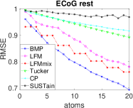
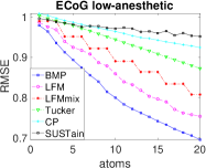
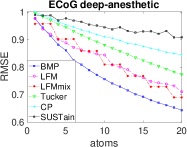
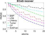
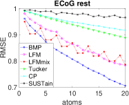
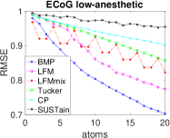
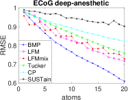
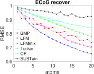
Figure 2: Performance comparison w.r.t number of atoms on real-world ECoG datasets for different methods. Top: denoising RMSE. Bottom: completion RMSE.

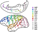
Figure 3: Bipolar ECoG electrode arrays. MP: Medial prefrontal cortex, LP: Lateral prefrontal cortex, PM: Premotor cortex, MS: Primary motor and somatosensory cortices, PC: Parietal cortex, TC: Temporal cortex, HV: Higher visual cortex and LV: Lower visual cortex.

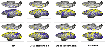
Figure 4: Boolean factors of two atoms: atom 2 (top row) and atom 4 (bottom row) learn from BCI datasets corresponding to different monkey brain consciousness conditions. Factors are color coded (Yellow for 1 and blue for 0), indicating the presence or absence of certain latent features.

7 Conclusion

We proposed an efficient optimization algorithm BMP for solving tensor decomposition with Boolean factors, leveraging atomic norm regularization and Boolean quadratic program. We proved that BMP can achieve sublinear convergence and polynomial run-time and sample complexity. We experimented exhaustively on synthetic and real-world datasets and observed superior performance for both tensor denoising and recovery tasks. When applied to ECoG recording, our method reveals the interesting neural mechanism underlying brain consciousness conditions.

8 Appendix

A. Proof of Theorem 1

Given an atomic set of rank-1 tensors $\mathds{A}=\bigcup\mathds{A}_{n}$, where $\mathds{A}_{n}=\{\mathcal{M}|\mathcal{M}=\boldsymbol{z}^{r}_{n}\otimes\boldsymbol{u}^{r}_{n}\otimes\boldsymbol{w}^{r}_{n}\}$, the span of an atomic set is defined as the linear combination of the atoms in the set:

$$span(\mathds{A})=\{\mathcal{W}\mid\mathcal{W}=\sum_{\mathcal{M}_{k}\in\mathds{A}}\boldsymbol{c}_{k}\mathcal{M}_{k},\;\boldsymbol{c}\in\mathbb{R}^{|\mathds{A}|}\}$$

The orthogonal projection of the set is:

$$\Delta\mathcal{W}_{\bot}:=\mathbf{proj}_{span(\mathds{A})^{\bot}}(\Delta\mathcal{W}),\quad\mathcal{M}_{\bot}:=\mathbf{proj}_{span(\mathds{A})^{\bot}}(\mathcal{M}),$$

to denote projection onto the orthogonal space of the span of the active set of atoms $\mathds{A}$ at the beginning of the iteration. The atomic norm of a tensor $\mathcal{W}$ with arbitrary Boolean factors is:

$$\|\mathcal{W}\|_{\mathds{A}}=\big{\{}\inf\ \|\boldsymbol{c}\|_{1}:\mathcal{W}=\sum_{\mathcal{M}_{k}\in\mathds{A}}\boldsymbol{c}_{k}\mathcal{M}_{k},\mathcal{M}=\boldsymbol{z}^{r}\otimes\boldsymbol{u}^{r}\otimes\boldsymbol{w}^{r}\big{\}}$$

Let $\mathcal{M}^{\star}$ be the atom selected by the Algorithm, the following lemma shows that minimization of a linear function with an atomic-norm regularization is achieved by minimization w.r.t. the greedy atomic direction.

Lemma 1.

Given a tensor $C$ and $\mathcal{W}$, the following equality holds:

$$\min_{\mathcal{W}\in\mathbb{V}}\;\langle C,\mathcal{W}\rangle+\frac{\beta}{2}\|\mathcal{W}\|_{\mathds{A}}^{2}=\min_{\boldsymbol{c}}\;\langle C,\boldsymbol{c}\mathcal{M}^{*}_{\bot}\rangle+\frac{\beta}{2}\|\boldsymbol{c}\mathcal{M}^{*}_{\bot}\|_{\mathds{A}}^{2}$$

where $\mathbb{V}$ is some linear subspace, $\mathcal{M}^{*}_{\bot}=\mathbf{proj}_{\mathbb{V}}(\mathcal{M})$, and $\boldsymbol{c}\in\mathbb{R}^{|\mathds{A}|}$ is the weight vector.

Proof.

The minimization problem with an atomic norm regularization

$$\min_{\mathcal{W}\in\mathbb{V}}\;\langle C,\mathcal{W}\rangle+\frac{\beta}{2}\|\mathcal{W}\|_{\mathds{A}}^{2}$$ (13)

is equivalent to the constrained minimization problem

$$\min_{\mathcal{W}\in\mathbb{V}}\; \langle C,\mathcal{W}\rangle s.t. \|\mathcal{W}\|_{\mathds{A}}\leq\delta$$ (14)

for some constant $\delta$. Since the problem of form (14) involves a linear objective function with a convex constraint, it always has an optimal solution that lies on the boundary of the atomic-norm constraint set. Therefore, there is always a solution to (13) of the form $\mathcal{W}=c\mathcal{M}^{*}_{\bot}$. ∎

Now we state the proof for Theorem 1.

Proof.

Let $F$ be a $\beta$-smooth loss function w.r.t the solution $\mathcal{W}$, its gradient is $\beta$-Lipschitz, we have

$$F(\mathcal{W}^{\prime})-F(\mathcal{W})\leq\langle\nabla F(\mathcal{W}),\mathcal{W}^{\prime}-\mathcal{W}\rangle+\frac{\beta}{2}\|\mathcal{W}^{\prime}-\mathcal{W}\|^{2}_{F}.$$ (15)

At $(k+1)$-th iteration, we greedily add a new atom $\mathcal{M}^{*}\leftarrow\operatorname*{arg\,min}_{n}\langle\nabla F(\mathcal{W}),\mathcal{M}_{n}\rangle$ into the active set $\mathds{A}^{k}$. A key ingredient of our analysis is the $\mu=3/5$ constant-approximation guarantee in the greedy step given by the SDP-based MAXCUT solver, where we have the following guarantee:

$$\langle\nabla F(\mathcal{W}),\mathcal{M}^{*}\rangle\leq\min_{n}\langle\nabla F(\mathcal{W}),\mathcal{M}_{n}\rangle\leq\mu\min_{n}\min_{\mathcal{M}_{n}\in\mathds{A}_{n}}\langle\nabla F(\mathcal{W}),\mathcal{M}_{n}\rangle=\min_{\mathcal{M}\in\mathds{A}}\langle\nabla F(\mathcal{W}),\mathcal{M}\rangle$$

After the fully-corrective weight adjustment in (9), we have

$$F(\mathcal{W}^{k+1})=\min_{\mathcal{W}\in span(\mathds{A}^{k+1})}F(\mathcal{W})\leq\min_{c\in\mathbb{R}}\;F(\mathcal{W}^{k}+c\mathcal{M}_{\bot}^{*})$$

for some constant $c$, given that $\mathcal{W}^{k}+c\mathcal{M}_{\bot}^{*}\in span(\mathds{A}^{k+1})$.

$$F(\mathcal{W}^{k+1})-F(\mathcal{W}^{k})\leq \min_{c\in\mathbb{R}}\;F(\mathcal{W}^{k}+c\mathcal{M}_{\bot}^{*})-F(\mathcal{W}^{k})$$ (16)

$$\leq \min_{c\in\mathbb{R}}\;\langle\nabla F(\mathcal{W}^{k}),c\mathcal{M}_{\bot}^{*}\rangle+\frac{\beta}{2}\|c\mathcal{M}^{*}_{\bot}\|_{\mathds{A}}^{2}$$

By lemma 1, we have

$$\min_{c}\;\langle\nabla F(\mathcal{W}^{k}),c\mathcal{M}^{*}_{\bot}\rangle+\frac{\beta}{2}\|c\mathcal{M}^{*}_{\bot}\|_{\mathds{A}}^{2} =\min_{n}\min_{\Delta\mathcal{W}\in span(\mathds{A}^{k}_{n})^{\bot}}\;\langle\nabla F(\mathcal{W}^{k}),\Delta\mathcal{W}\rangle+\frac{\beta}{2}\|\Delta\mathcal{W}\|_{{\mathds{A}}^{2}_{n}}$$

Note that since $\langle\nabla F(\mathcal{W}^{k}),\Delta\mathcal{W}\rangle=0$ for any $\Delta W\in span(\mathds{A}^{k}_{n})$, we also have

$$\min_{n}\min_{\Delta\mathcal{W}\in span(\mathds{A}^{k}_{n})^{\bot}}\;\langle\nabla F(\mathcal{W}^{k}),\Delta\mathcal{W}\rangle+\frac{\beta}{2}\|\Delta\mathcal{W}\|_{{\mathds{A}}^{2}_{n}}$$

$$=\min_{\Delta\mathcal{W}\in span(\mathds{A})}\;\langle\nabla F(\mathcal{W}^{k}),\Delta\mathcal{W}\rangle+\frac{\beta}{2}\|\Delta\mathcal{W}_{\bot}\|_{\mathds{A}}^{2}.$$

By constraining $\Delta W$ to be of the form $\Delta W=\alpha(\mathcal{W}^{*}-\mathcal{W}^{k})$ , we have

$$\min_{n}\min_{\Delta\mathcal{W}\in span(\mathds{A}_{n})^{\bot}}\;\langle\nabla F(\mathcal{W}^{k}),\Delta\mathcal{W}\rangle+\frac{\beta}{2}\|\Delta\mathcal{W}_{\bot}\|_{{\mathds{A}}^{2}_{n}}$$

$$\leq\min_{\Delta\mathcal{W}=\alpha(\mathcal{W}^{*}-\mathcal{W}^{k}),\alpha\in[0,1]}\;\mu\langle\nabla F(\mathcal{W}^{k}),\Delta\mathcal{W}\rangle+\frac{\beta}{2}\|\Delta\mathcal{W}_{\bot}\|_{\mathds{A}}^{2}$$

$$\leq\min_{\alpha\in[0,1]}\;\alpha\mu(F(\mathcal{W}^{*})-F(\mathcal{W}^{k}))+\frac{\beta\alpha^{2}}{2}\|\mathcal{W}^{*}_{\bot}\|_{\mathds{A}}^{2}$$

where the second inequality is from convexity. Let $F^{*}:=F(\mathcal{W}^{*})$, minimize over $\alpha$, we have

$$(F(\mathcal{W}^{k+1})-F^{*})-(F(\mathcal{W}^{k})-F^{*})$$

$$\leq\min\{\frac{\mu^{2}}{2\beta\|\mathcal{W}^{*}\|_{\mathds{A}}^{2}}(F(\mathcal{W}^{k})-F^{*})^{2},\frac{\mu}{2}(F(\mathcal{W}^{k})-F^{*})\}$$

The recurrence then leads to the convergence result:

$$F(\mathcal{W}^{k})-F^{*}\leq\frac{2\beta\|\mathcal{W}^{*}\|_{\mathds{A}}^{2}}{\mu^{2}}\frac{1}{k}$$

∎

B. Proof of Theorem 2

Proof.

Denote the support set $\bar{A}\subset[\bar{K}]$, meaning $\boldsymbol{c}_{j}=0$ for $j\notin\bar{A}$. Define $\boldsymbol{c}_{\bar{A}}:=\{\boldsymbol{c}_{k}\}_{k\in\bar{A}}$ and $f(\boldsymbol{c}_{\bar{A}}):=F(\sum_{k\in\bar{A}}c_{k}\mathcal{M}_{k}).$ Suppose $f(\boldsymbol{c}_{\bar{A}})$ is strongly convex with respect to $\bar{A}$ with parameter $\gamma$. Since $\boldsymbol{c}^{*}$ is the minimizer of $f(\boldsymbol{c})$, it satisfies $\langle\nabla f(\boldsymbol{c}^{*}),\boldsymbol{c}^{*}\rangle=0$ and thus

$$f(0)-f(\boldsymbol{c}^{*}) =f(0)-f(\boldsymbol{c}^{*})-\langle\nabla f(\boldsymbol{c}^{*}),0-\boldsymbol{c}^{*}\rangle$$

$$\geq\frac{\gamma}{2}\|\boldsymbol{c}^{*}\|^{2}.$$

Since, $f(0)-f(\boldsymbol{c}^{*})\leq\frac{1}{2}\|\mathcal{X}\|_{F}^{2}$, we have

$$\|\mathcal{W}^{*}\|_{\mathds{A}}^{2}=\|\boldsymbol{c}^{*}\|_{1}^{2}\leq\bar{K}\|\boldsymbol{c}^{*}\|_{2}^{2}\leq\frac{\bar{K}\|\mathcal{X}\|_{F}^{2}}{\gamma}.$$ (17)

Substituting (14) into (10) yields the result (12). ∎

C. Proof of Theorem 3

The following Kruskal’s condition [31] guarantees the uniqueness of generic tensor decomposition:

Condition 3 (Kruskal).

An order-3 rank-R tensor of dimension $d_{1}\times d_{2}\times d_{3}$ is unique if

$$R\leq\frac{1}{2}\left(\text{krank}(\mathbf{Z})+\text{krank}(\mathbf{U})+\text{krank}(\mathbf{W})-2\right)$$

where $\text{krank}(\cdot)$ is the largest value of a matrix such that every subset of columns of the matrix is linearly independent. It is also easy to see that $\text{krank}(\mathbf{Z})\leq\text{rank}(\mathbf{Z})$ for any $\mathbf{Z}$.

To guarantee uniqueness of the Boolean factor $\mathbf{Z}$, we need the following condition on its column vectors vectors $\{\boldsymbol{z}_{r}\}$ to hold.

Condition 4.

The tensor decomposition problem has unique Boolean factors if for any non-trivial combinations of the column vectors $\{\boldsymbol{z}_{r}\}$ would lead to a non-Boolean vector:

$$\forall\boldsymbol{c}\neq\boldsymbol{0},\quad\boldsymbol{c}^{\top}\boldsymbol{Z}\in\mathbb{Z}_{2}\iff\boldsymbol{c}\in\{\boldsymbol{e}_{i}\}$$

which means the linear subspace of $\boldsymbol{Z}^{n}$ does not contain any other Boolean vectors that are not already in $\mathbf{Z}^{n}$. This identifiability condition is in nature similar to [13].

A tensor decomposition $\mathcal{W}=\sum_{r=1}^{R}\boldsymbol{z}_{r}\otimes\boldsymbol{u}_{r}\otimes\boldsymbol{w}_{r}$ is said to be unique if for any other decomposition, $\mathcal{W}=\sum_{r=1}^{R}\boldsymbol{z}_{r}^{\prime}\otimes\boldsymbol{u}_{r}^{\prime}\otimes\boldsymbol{w}_{r}^{\prime}$, there exists a permutation $\sigma$ such that

$$\boldsymbol{z}_{r}\otimes\boldsymbol{u}_{r}\otimes\boldsymbol{w}_{r}=\boldsymbol{z}_{\sigma(r)}^{\prime}\otimes\boldsymbol{u}_{\sigma(r)}^{\prime}\otimes\boldsymbol{w}_{r}^{\prime}$$

When tensor $\mathcal{W}$ has a unique decomposition, the set of vectors $\boldsymbol{z}$ , $\boldsymbol{u}$ and $\boldsymbol{w}$ are identifiable, up to scalars. Let $\mathbf{Z}$ be the matrix containing $\boldsymbol{z}_{r}$ as its columns. Similarly for matrices $\mathbf{U}$ and $\mathbf{W}$.

Proof.

Suppose all the continues-valued factors are normalized, with $\|\boldsymbol{u}\|_{2},\|\boldsymbol{w}\|_{2}\leq 1$. The optimization problem of parameter recovery without noise is equivalent to

$$\min_{\boldsymbol{c}}\|\boldsymbol{c}\|_{1}\quad\text{s.t.}\quad\mathcal{X}=\sum_{k=1}^{\bar{K}}\boldsymbol{c}_{k}\mathcal{M}_{k},\mathcal{M}_{k}=\boldsymbol{z}_{k}\otimes\boldsymbol{u}_{k}\otimes\boldsymbol{w}_{k}$$ (18)

where $\bar{K}$ is the size of the atom set $\mathds{A}$. The problem in (18) has a unique solution $\boldsymbol{c}^{\star}$, which selects the true atoms as $\{\mathcal{M}_{k}^{\star}=\boldsymbol{z}_{k}^{\star}\otimes\boldsymbol{u}_{k}^{\star}\otimes\boldsymbol{w}_{k}^{\star}\}$. Under the identifiability conditions, the tensor decomposition is unique up to scalars. For any solution returned by the algorithm $\{\mathcal{M}=\boldsymbol{z}_{k}\otimes\boldsymbol{u}_{k}\otimes\boldsymbol{w}_{k}\}$, there exists a permutation $\sigma$, such that $\boldsymbol{u}^{\star}_{k}=\boldsymbol{u}_{\sigma(k)}$ and $\boldsymbol{w}^{\star}_{k}=\boldsymbol{w}_{\sigma(k)}$. Given that the Boolean factors are unique by Condition (4), $\mathcal{M}_{k}$ is rank-1 and we can recovery $\boldsymbol{u}_{k}$ and $\boldsymbol{w}$ exactly. Therefore, the linear subspace spanned by $\{\boldsymbol{u}_{k}\}$ is the same as that of $\{\boldsymbol{u}^{\star}_{k}\}$, similar for $\{\boldsymbol{w}_{k}\}$.

∎

D. Proof of Theorem 4

Definition 1 (Restricted Strongly Convex (RSC)).

For a given tensor $\mathcal{W}$, we say the loss function $F(\mathcal{W})$ is restricted strongly convex with parameter $\kappa$, if

$$\|\triangledown F(\mathcal{W})\|_{op}\geq\kappa\|\mathcal{W}\|_{F}^{2}$$

where $\|\cdot\|_{2}$ is the spectral norm and $\|\cdot\|_{F}$ is the Frobenius norm.

It is easy to see that given the atomic set of rank-1 tensors, the atomic norm of the tensor $\|\mathcal{W}\|_{\mathds{A}}$ is equivalent to the tensor nuclear norm. Consider the case where the tensor decomposition has orthogonal factors. That is $\mathbf{Z}^{\top}\mathbf{Z}=\mathbf{I}$ $\mathbf{U}^{\top}\mathbf{U}=\mathbf{I}$ and $\mathbf{W}^{\top}\mathbf{W}=\mathbf{I}$ obtained through orthogonalization, we have:

$$\|\mathcal{W}\|_{\mathds{A}}=\{\inf\|\boldsymbol{c}\|_{1}\ |\ \mathcal{W}=\boldsymbol{c}_{k}\boldsymbol{z}_{k}\otimes\boldsymbol{u}_{k}\otimes\boldsymbol{w}_{k}\}=\{\inf_{\boldsymbol{\sigma}}\|\boldsymbol{\sigma}\|_{1}\ |\ \mathcal{W}={\sigma}_{r}\boldsymbol{z}_{k}\otimes\boldsymbol{u}_{k}\otimes\boldsymbol{w}_{k},\langle\boldsymbol{z}_{i},\boldsymbol{z}_{j}\rangle=0\}$$

Given the statistical estimation problem of sample size $S$:

$$\hat{\mathcal{W}}=\min_{\mathcal{W}}\mathbb{E}[\frac{1}{2S}F_{i}(\mathcal{W})+\lambda\|\mathcal{W}\|_{\mathds{A}}]$$

where per sample loss $F_{i}(\mathcal{W})$ is defined as $F_{i}(\mathcal{W})=\|\mathfrak{X}(\mathcal{X}_{i}-\mathcal{W})\|_{F}$. $\mathfrak{X}$ is a linear operator representing vectorization or random sampling. Assume the true low-rank tensor parameter is $\mathcal{W}^{\star}$, the statistical estimation difference $\hat{\Delta}:=\hat{\mathcal{W}}-\mathcal{W}^{\star}$ can be decomposed into two parts: components that are in the span of $\mathds{A}$, denoted as $\Delta$ and the components that are in the complement of $\mathds{A}$, denoted as $\Delta_{\bot}$. As the atomic norm is decomposable w.r.t the subspace of $\mathds{A}$, we have $\hat{\Delta}=\Delta+\Delta_{\bot}$ and $\|\hat{\Delta}\|_{\mathds{A}}=\|\Delta\|_{\mathds{A}}+\|\Delta_{\bot}\|_{\mathds{A}}$. The following lemma relates the atomic norm of these two components.

Lemma 2.

Let the estimation error be $\|\mathfrak{X}(\hat{\Delta})\|_{F}=\|\mathfrak{X}(\hat{\mathcal{W}}-\mathcal{W}^{\star})\|_{F}$ satisfying $\hat{\Delta}=\Delta+\Delta_{\bot}$, where $\Delta=\text{proj}_{\mathds{A}}(\hat{\Delta})$ and $\Delta_{\bot}$ is the projection onto the complement of $\mathds{A}$. If the regularization $\lambda$ satisfy $\lambda\geq 2\|\triangledown F(\mathcal{W})\|_{\mathds{A}}$, we have $\text{rank}(\Delta)\leq 2R$ and $\|\Delta_{\bot}\|_{\mathds{A}}\leq 3\|\Delta\|_{\mathds{A}}$.

Proof.

Since the true model is low-rank $\mathcal{W}^{\star}\in\mathds{A}$ based on our algorithm and the atomic norm $\|\cdot\|_{\mathds{A}}$ is decomposable w.r.t. the rank-1 tensors. Proof follows similarly from Lemma 1 in [32].

By Hölder’s inequality and triangle inequality, we have

$$\frac{1}{2S}\|\mathfrak{X}(\hat{\Delta})\|_{F}^{2}\leq\frac{1}{S}\langle\mathfrak{X}(\mathcal{E}),\hat{\Delta}\rangle+\lambda_{S}\|\hat{\Delta}\|_{\mathds{A}}\leq\frac{1}{S}\|\mathfrak{X}(\mathcal{E})\|_{op}\|\hat{\Delta}\|_{\mathds{A}}+\lambda_{S}\|\hat{\Delta}\|_{\mathds{A}}\leq 2\lambda_{S}\|\hat{\Delta}\|_{\mathds{A}}$$ (19)

With the choice of $\lambda_{S}\geq\|\mathfrak{X}(\mathcal{E})\|_{op}/S$. By Lemma 2, we have

$$\|\hat{\Delta}\|_{\mathds{A}}=\|\Delta\|_{\mathds{A}}+\|\Delta_{\bot}\|_{\mathds{A}}\leq 4\|\Delta_{\bot}\|_{\mathds{A}}\leq 4\|\Delta\|_{F}\sqrt{2R}$$ (20)

By Definition 1, we have the lower bound $\frac{1}{2S}\|\mathfrak{X}(\Delta)\|_{F}^{2}\geq\kappa(\mathfrak{X})\|\Delta\|_{F}^{2}$ with $\kappa(\mathfrak{X})$ as the RSC constant of the linear operator $\mathfrak{X}$. Combining Eqn. (19) and (20), we have $\|\hat{\Delta}\|_{F}\leq 8\lambda_{S}\sqrt{2R}/\kappa$.

For i.i.d Gaussian noise $\mathcal{E}\sim\mathcal{N}(0,\sigma^{2})$, apply concentration bound. There exists a universal constant $c_{1}$ such that:

$$\|\mathfrak{X}(\mathcal{E})\|_{op}^{2}\leq\mathcal{O}_{p}\big{(}c_{1}\sigma^{2}R(d_{1}+d_{2}+d_{3})\big{)}.$$ (21)

Combine Eqn. (19), (20) and (21) together, the following statically bound for the estimation error holds for some constant $c_{1}$ with high probability:

$$\|\mathfrak{X}(\hat{\mathcal{W}}-\mathcal{W}^{\star})\|_{F}^{2}\leq\mathcal{O}_{p}\big{(}c_{1}\frac{\sigma^{2}R(d_{1}+d_{2}+d_{3})}{S}\big{)}$$

which is proportional to the noise variance and the degree of freedom in the tensor model. ∎

References

- [1] Animashree Anandkumar, Rong Ge, Daniel Hsu, Sham M Kakade, and Matus Telgarsky. Tensor decompositions for learning latent variable models. The Journal of Machine Learning Research, 15(1):2773–2832, 2014.
- [2] Rose Yu, Mohammad Taha Bahadori, and Yan Liu. Fast Multivariate Spatio-temporal Analysis via Low Rank Tensor Learning. In NIPS, 2014.
- [3] Alex H Williams, Tony Hyun Kim, Forea Wang, Saurabh Vyas, Stephen I Ryu, Krishna V Shenoy, Mark Schnitzer, Tamara G Kolda, and Surya Ganguli. Unsupervised discovery of demixed, low-dimensional neural dynamics across multiple timescales through tensor component analysis. Neuron, 98(6):1099–1115, 2018.
- [4] Tammo Rukat, Chris Holmes, and Christopher Yau. Probabilistic boolean tensor decomposition. In International conference on machine learning, pages 4410–4419, 2018.
- [5] Ioakeim Perros, Evangelos E Papalexakis, Haesun Park, Richard Vuduc, Xiaowei Yan, Christopher Defilippi, Walter F Stewart, and Jimeng Sun. Sustain: Scalable unsupervised scoring for tensors and its application to phenotyping. In ACM KDD, 2018.
- [6] Vin De Silva and Lek-Heng Lim. Tensor rank and the ill-posedness of the best low-rank approximation problem. SIAM Journal on Matrix Analysis and Applications, 30(3):1084–1127, 2008.
- [7] Hsiao-Yu Tung and Alexander J Smola. Spectral methods for indian buffet process inference. In Advances in Neural Information Processing Systems, pages 1484–1492, 2014.
- [8] Ariel Jaffe, Roi Weiss, Shai Carmi, Yuval Kluger, and Boaz Nadler. Learning binary latent variable models: A tensor eigenpair approach. arXiv preprint arXiv:1802.09656, 2018.
- [9] Rong Ge and Tengyu Ma. On the optimization landscape of tensor decompositions. In Advances in Neural Information Processing Systems, pages 3653–3663, 2017.
- [10] Ryota Tomioka, Taiji Suzuki, Kohei Hayashi, and Hisashi Kashima. Statistical performance of convex tensor decomposition. In Advances in neural information processing systems, pages 972–980, 2011.
- [11] Ming Yuan and Cun-Hui Zhang. On tensor completion via nuclear norm minimization. Foundations of Computational Mathematics, 16(4):1031–1068, 2016.
- [12] Kishan Wimalawarne and Hiroshi Mamitsuka. Efficient convex completion of coupled tensors using coupled nuclear norms. In Advances in Neural Information Processing Systems, pages 6902–6910, 2018.
- [13] Martin Slawski, Matthias Hein, and Pavlo Lutsik. Matrix factorization with binary components. In Advances in Neural Information Processing Systems, pages 3210–3218, 2013.
- [14] Ian En-Hsu Yen, Wei-Cheng Lee, Sung-En Chang, Arun Sai Suggala, Shou-De Lin, and Pradeep Ravikumar. Latent feature lasso. In International Conference on Machine Learning, pages 3949–3957, 2017.
- [15] Saskia Metzler and Pauli Miettinen. Clustering boolean tensors. Data mining and knowledge discovery, 29(5):1343–1373, 2015.
- [16] Tamara G Kolda and Brett W Bader. Tensor decompositions and applications. SIAM review, 51(3):455–500, 2009.
- [17] Prateek Jain and Sewoong Oh. Provable tensor factorization with missing data. In Advances in Neural Information Processing Systems, pages 1431–1439, 2014.
- [18] Vatsal Sharan and Gregory Valiant. Orthogonalized als: A theoretically principled tensor decomposition algorithm for practical use. In Proceedings of the 34th International Conference on Machine Learning-Volume 70, pages 3095–3104. JMLR. org, 2017.
- [19] Silvia Gandy, Benjamin Recht, and Isao Yamada. Tensor completion and low-n-rank tensor recovery via convex optimization. Inverse Problems, 27(2):025010, 2011.
- [20] Ryota Tomioka and Taiji Suzuki. Convex tensor decomposition via structured schatten norm regularization. In Advances in neural information processing systems, pages 1331–1339, 2013.
- [21] Pauli Miettinen. Boolean tensor factorizations. In Data Mining (ICDM), 2011 IEEE 11th International Conference on, pages 447–456. IEEE, 2011.
- [22] Piyush Rai, Changwei Hu, Matthew Harding, and Lawrence Carin. Scalable probabilistic tensor factorization for binary and count data. In IJCAI, pages 3770–3776, 2015.
- [23] Zoubin Ghahramani and Thomas L Griffiths. Infinite latent feature models and the indian buffet process. In Advances in neural information processing systems, pages 475–482, 2006.
- [24] Kenneth Kreutz-Delgado, Joseph F Murray, Bhaskar D Rao, Kjersti Engan, Te-Won Lee, and Terrence J Sejnowski. Dictionary learning algorithms for sparse representation. Neural computation, 15(2):349–396, 2003.
- [25] Venkat Chandrasekaran, Benjamin Recht, Pablo A. Parrilo, and Alan S. Willsky. The Convex Geometry of Linear Inverse Problems. Foundations of Computational Mathematics, 2012.
- [26] Stéphane Mallat and Zhifeng Zhang. Matching pursuit with time-frequency dictionaries. Technical report, Courant Institute of Mathematical Sciences New York United States, 1993.
- [27] Joel A Tropp, Anna C Gilbert, and Martin J Strauss. Algorithms for simultaneous sparse approximation. part i: Greedy pursuit. Signal processing, 86(3):572–588, 2006.
- [28] Michael R Garey and David S Johnson. Computers and intractability, a guide to the theory of np-completness. 1979.
- [29] Yurii Nesterov. Quality of semidefinite relaxation for nonconvex quadratic optimization. Technical report, Université catholique de Louvain, Center for Operations Research and Econometrics (CORE), 1997.
- [30] Po-Wei Wang, Wei-Cheng Chang, and J Zico Kolter. The mixing method: coordinate descent for low-rank semidefinite programming. arXiv preprint arXiv:1706.00476, 2017.
- [31] Joseph B Kruskal. Three-way arrays: rank and uniqueness of trilinear decompositions, with application to arithmetic complexity and statistics. Linear algebra and its applications, 18(2):95–138, 1977.
- [32] Sahand N Negahban, Pradeep Ravikumar, Martin J Wainwright, Bin Yu, et al. A unified framework for high-dimensional analysis of -estimators with decomposable regularizers. Statistical Science, 27(4):538–557, 2012.
- [33] Joel A Tropp and Anna C Gilbert. Signal recovery from random measurements via orthogonal matching pursuit. IEEE Transactions on information theory, 53(12):4655–4666, 2007.
- [34] Lieven De Lathauwer, Bart De Moor, and Joos Vandewalle. A multilinear singular value decomposition. SIAM journal on Matrix Analysis and Applications, 21(4):1253–1278, 2000.
- [35] Toru Yanagawa, Zenas C Chao, Naomi Hasegawa, and Naotaka Fujii. Large-scale information flow in conscious and unconscious states: an ecog study in monkeys. PloS one, 8(11):e80845, 2013.