Non–local interactions in the surrogate method for reactions
Abstract
- Background
-
Single-neutron transfer reactions populating states in the continuum are interesting both for structure and astrophysics. In their description often global optical potentials are used for the nucleon-target interactions, and these interactions are typically local. In our work, we study the effects of nonlocality in reactions populating continuum states. This work is similar to that of [1] but now for transfer to the continuum.
- Purpose
-
A theory for computing cross sections for inclusive processes was explored in [2]. Therein, local optical potentials were used to describe the nucleon-target effective interaction. The goal of the present work is to extend the theory developed in [2] to investigate the effects of including nonlocality in the effective interaction on the relevant reaction observables.
- Method
-
We implement the R–matrix method to solve the non–local equations both for the nucleon wavefunctions and the propagator. We then apply the method to systematically study the inclusive process of on 16O, 40Ca, 48Ca and 208Pb at 10, 20 and 50 MeV. We compare the results obtained when non–local interactions are used with those obtained when local equivalent interactions are included.
- Results
-
We find that nonlocality affects different pieces of the model in complex ways. The competition between the reduction of the propagator and the neutron wavefunction in the region of interest and the increase of the magnitude of the interaction produces varying effects on the cross section. Depending on the beam energy and the target, the non-elastic breakup can either increase or decrease. Effects on the heavier targets can be as large as %.
- Conclusions
-
While the non-elastic transfer cross section for each final spin state can change considerably, the main prediction of the model [2], namely the shape of the spin distributions, remains largely unaltered by nonlocality.
I Motivation
Neutron capture reactions are an essential piece of the puzzle in understanding the formation of nuclei heavier than 56Fe [3]. One of the major efforts in our community is understanding the -process [4] which requires neutron capture rates for short-lived isotopes. Neutron capture reactions are also relevant to new reactor designs and for stockpile stewardship [5, 6]. For many of these applications, the isotopes are sufficiently far from stability that it is impossible to measure directly and indirect methods need to be used.
This work is focused on the use of reactions as a surrogate for . Many of the isotopes in the -process path are unstable but not close to the neutron drip line. For these isotopes, resonant capture is the dominant capture process. In resonant neutron capture, the neutron populates compound excited states in the continuum, and then decays through -ray or particle emission. Any indirect method for assumes that it populates the same compound states. In the surrogate method, it is assumed that the deuteron will transfer its neutron onto the target, forming the same compound nucleus that is formed in the direct , so that, by measuring the -decay following the reaction, one can constrain the neutron capture of interest. However, one does need to rely on reaction theory for a reliable extraction [7, 8, 9, 2, 10].
There are some known complications to the extraction. The model described in [2] relies on a 2-step process, first the deuteron breaks up and then the neutron gets captured (absorbed) by the target. But, in this model, there is some probability that the neutron will not be absorbed, leading to elastic breakup (EB). The EB cross section needs to be subtracted from the total cross section. The remaining component, usually called the non-elastic breakup (NEB), connects with the compound nucleus formation in reactions. One of the most important inputs that theory provides in the analysis of the surrogate data are the spin distributions, essential for correcting the weights of the various final spins to enable a reliable extraction of the cross section. It turns out that the spin distribution obtained through is not the same as that obtained in . An example of a successful application of the method can be found in [11].
Up to now, the models of surrogate reactions [7, 8, 9, 2, 10] have used local nucleon-target optical potentials. However, it is well known that the nucleon-nucleus effective interactions are non–local due to the channel couplings and antisymmetrization of many-body wavefunctions (e.g. [12, 13, 14, 15, 16]). In the last decade, there has been a considerable amount of effort to develop microscopic optical potentials which are intrinsically non–local. An example is the dispersive optical model (DOM) theory which was first introduced by Mahaux and Sartor [17] and has been implemented and applied by the St. Louis group [18]. Another approach is to obtain the optical potential using ab initio methods. An example of a recent effort using Coupled Cluster theory is discussed in [19]. Although the work in [19] demonstrates that ab initio optical potentials are still not of practical use, it is important to incorporate, in the implementation of the reaction theory for surrogates, the capability of dealing with non–local interactions. Furthermore, it is crucial to study the effects of nonlocality in the predictions for the surrogate process to determine whether future analyses need to take this aspect into account.
A study of the effects of nonlocality on reaction observables has a long history, including the well known works of Austern [20, 21] and Fiedeldey [22] (codes like TWOFNR [23] and DWUCK [24] contain such non–local corrections) . This topic has been recently revisited [1, 25]. In [1] nonlocality was only included in the nucleon channels, both in calculating the neutron bound-state wavefunction and the proton distorted wave. Nonlocality had opposing effects on these two wavefunctions. The largest effect was the reduction of the neutron wavefunction in the interior which, due to normalization, produced an increase of the peripheral part. This resulted in an overall increase of the transfer cross section when non–local interactions were included. The method was then generalized to include nonlocality in the deuteron channel [25]. Whether using the distorted wave approximation (DWBA) or the adiabatic wave approximation (ADWA), nonlocality was found to have a considerable effect on transfer angular distributions, mostly affecting the magnitude but sometimes also the shape. Given these results, one might expect similar effects in reactions populating continuum states. Here we will use the non–local optical potential derived by Perey and Buck [26] to make it easier to compare with previous work [1, 25]. However, it is understood that the actual non–local optical potential from nature is not simply of Gaussian form and should still contain some energy dependence [27]. The energy dependence is usually interpreted as a consequence of the coupling with collective states, and it tends to give rise to a longer–range non–locality.
The work performed in [1, 25] made use of an iterative method for solving the non–local Schödinger equation [28]. However this method is not very efficient and this became a serious issue when considering transfer to the continuum which involves the computation of a whole range of neutron scattering final states. For this reason, and in order to complete this project, we implemented a modified R–matrix method following the work by Descouvemont and Baye [29]. Transforming the finite differences problem into a linear algebra problem provided three orders of magnitude improvement in computing time for the calculations involving non–local interactions [30].
Following the systematic study of [1, 25], we study the non-elastic breakup on 16O, 40Ca, 48Ca and 208Pb, at various beam energies (10, 20 and 50 MeV). The results obtained using non–local optical potentials are compared with those obtained using local equivalent potentials (LEP). We look at the direct NEB term (Udagawa term [31]) as well as the non–orthogonality term (Hussein and McVoy term [32]). We also consider the spin distributions in detail.
In section II, we provide a brief theoretical background, including a summary of the formalism of [2] and the details of the R–matrix method as we implemented it. Next, in Section III we provide the numerical details associated with our calculations. This is followed by the results in Section IV. The conclusions are drawn in Section VI.
II Theoretical background
II.1 Inclusive reactions
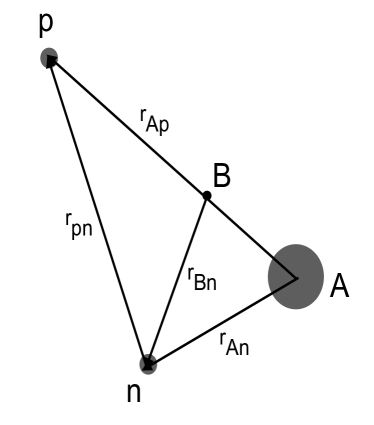
In this work we describe the NEB channels populated in processes within a two–step mechanism. The first step consists in the breaking up of the deuteron due to the action of the neutron–target potential, while, in the second step, the released neutron interacts with the target. We adopt the system of coordinates shown in Fig. 1 where represents a state of the system. The neutron–target interaction is described by the single–particle Green’s function , and results in the population of the elastic breakup and NEB final channels (the superscript opt is meant to indicate that the single–particle operator has been obtained by optical reduction of the many–body propagator , see [2]). For low neutron–target relative energies ( MeV), the compound nucleus formation dominates the NEB processes, and reactions can be used as surrogate for () reactions.
For negative neutron energies, and in the limit of the imaginary part of the neutron–target interaction going to zero, the NEB contribution can be shown to reproduce the standard DWBA with a neutron wavefunction generated by the real part of this interaction [2]. By focusing our attention on the NEB component of the reaction, we can then consider this work as a natural extension of [1] to positive energies, as well as describing the channel of interest for the surrogate method.
The nonelastic-breakup differential cross section can be expressed as [2]
| (1) |
In order to understand the various terms in Eq. (1) it is necessary to introduce some important ingredients of the theory. These include the proton level density:
| (2) |
where describes the kinetic energy of proton, and is the imaginary part of the neutron–target potential, which accounts for all reaction channels. The first term in Eq. (1) describes the direct (Udagawa–Tamura, UT [31]) process, and can be written as
| (3) |
while the second term corresponds to the nonorthogonality (Hussein–McVoy, HM) contribution [32],
| (4) |
The third term corresponds to the interference between the UT and HM contributions, testifying to fact that both terms contribute coherently to the total NEB cross section.
An important element in the theory is the neutron wavefunction, after breakup, in the field of the target:
| (5) |
This is the result of the application of the single–particle Green’s function (the propagator) to the source term
| (6) |
This source term accounts for the direct breakup of the deuteron, the first step in our two–step description. The deuteron distorted wave is generated by the local optical potential , while the proton scattering wavefunction is a positive–energy solution of a Schrödinger equation with the non–local potential (the round bracket on the left indicates integration over the proton coordinates only). Note that the neutron–target interaction is also, in general, non–local.
The non–orthogonality (Hussein–McVoy, HM) function is defined as
| (7) |
and accounts for the fact that, in prior form, there is an additional correction to the Udagawa-Tamura term [31].
In order to derive the Green’s function and the scattering wavefunction with non–local potentials, we have implemented dedicated numerical methods. We will briefly address them in the following sections. An extended description of this method will appear elsewhere [33].
II.2 R–matrix method
The proton scattering wavefunction is obtained by solving the non–local Schrödinger equation
| (8) |
where
| (9) |
and is the –component of the standard partial wave decomposition of . This equation has been solved with an iterative method by Titus et al. [28]. Here, we propose a faster and more robust method based on an R–matrix expansion [29].
The R–matrix method was first introduced by Wigner with the aim of describing resonances [34], and it has been developed and applied widely in atomic and nuclear physics [35, 36, 37]. The basic idea of the R–matrix method is to divide the configuration space into an internal () and an external region by defining a suitable radius . This limiting radius should be large enough so that the nuclear part of the interaction is negligible for . In practice, we check that the results are independent of the choice of . The boundary conditions can be conveniently enforced by defining the Bloch operator
| (10) |
and solving the associated integro–differential equation
| (11) |
The external wavefunction is a Coulomb wave:
| (12) |
where is the phase shift for partial wave , the Sommerfeld parameter, and is the proton wave number. The internal () wave function is expanded in the Lagrange basis:
| (13) |
The Lagrange functions are defined in the interval as
| (14) |
where (x) is a Legendre polynomial of degree , and the points verify
| (15) |
The factor enforces the regular behavior of the basis functions at the origin. The next step is to compute the Hamiltonian matrix in the Lagrange basis,
| (16) |
In the Lagrange basis, the local and non–local matrix elements present in the equation above are particularly easy to compute, without the need to perform any numerical integration (see [29]). The integro–differential equation (11) is thus recast into a linear algebra problem that can be solved for the coefficients of the expansion (13),
| (17) |
It is to be noted that this method can also be used to compute bound states, in which case the Coulomb wave functions enforcing the boundary conditions need be replaced by Whittaker functions.
II.3 Computing the Green’s function
The target–neutron Green’s function G can be written as
| (18) |
where stands for and stands for . Note that the Wronskian is –dependent when the potential is non–local. The function is the regular (irregular) solution of the non–local Schrödinger equation:
| (19) |
The regular solution for positive is obtained as described in the previous section, but taking an outgoing Coulomb wave as the boundary condition. On the other hand, the irregular solution cannot be expanded in the basis (14), since these Lagrange functions are regular at the origin. We use instead the alternative irregular basis defined in the interval ,
| (20) |
where we have dropped the factor , and . The generalization of the R–matrix method to arbitrary intervals with is described in [29], and we take advantage of the fact that the value of the irregular solution is known for small . We thus avoid to deal with the numerical difficulties associated with the divergent behavior of as . As we pointed out in the previous section, the Green’s function can also be computed for bound states by enforcing a Whittaker boundary condition for the regular solution.
III Numerical details
| LEP | ||||||||||
|---|---|---|---|---|---|---|---|---|---|---|
| A=16O | A=40Ca | A=208Pb | ||||||||
| En/ (MeV) | 2.500 | 14.000 | 3.000 | 7.000 | 3.000 | 15.000 | 10.000 | 40.000 | 3.500 | 14.000 |
| Vv (MeV) | 41.500 | 43.971 | 47.441 | 46.040 | 42.902 | 44.311 | 35.100 | 36.881 | 34.451 | 39.100 |
| rv (fm) | 1.340 | 1.311 | 1.271 | 1.291 | 1.270 | 1.290 | 1.261 | 1.271 | 1.250 | 1.253 |
| av (fm) | 0.601 | 0.620 | 0.671 | 0.62 | 0.640 | 0.619 | 0.632 | 0.616 | 0.601 | 0.615 |
| Wd (MeV) | 10.001 | 9.891 | 14.501 | 10.201 | 9.132 | 10.051 | 8.030 | 8.741 | 8.291 | 9.070 |
| rd (fm) | 1.290 | 1.262 | 1.361 | 1.240 | 1.281 | 1.250 | 1.241 | 1.243 | 1.232 | 1.241 |
| ad (fm) | 0.401 | 0.440 | 0.361 | 0.446 | 0.441 | 0.431 | 0.442 | 0.425 | 0.431 | 0.422 |
| Vso (MeV) | 7.180 | 0.000 | 7.180 | 0.000 | 7.180 | 0.000 | 7.180 | 0.000 | 7.180 | 0.000 |
| rso (fm) | 1.220 | — | 1.220 | — | 1.220 | — | 1.220 | — | 1.220 | — |
| aso (fm) | 0.650 | — | 0.650 | — | 0.650 | — | 0.650 | — | 0.650 | — |
| rc (fm) | 1.220 | 1.220 | 1.220 | 1.220 | 1.220 | 1.220 | 1.220 | 1.220 | 1.220 | 1.220 |
We performed a systematic study for on 16O, 40Ca, 48Ca and 208Pb at various beam energies, =10 MeV, 20 MeV and 50 MeV. The optical potential parameterization for and used in final proton and the neutron channel is the non–local Perey-Buck [26]. For the deuteron optical potential we have used a global phenomenological parametrization [38].
As in [1], in order to assess the effects of nonlocality, we compare those results with the calculations obtained using local equivalent potentials (LEP) for and . For each reaction studied (characterized by the target and the deuteron beam energy ), we estimate the neutron and proton energies corresponding to the the peak of the energy distribution of the NEB cross section. For those specific energies, we use sfresco [39] to fit the elastic scattering generated with the Perey-Buck potential, with a local interaction including a real volume Woods-Saxon term and an imaginary surface term (as in [1]). In the fitting, we do not fit the spin-orbit and Coulomb terms; these are fixed as in the Perey-Buck potential. Then, for each reaction, we use for the whole range of energies of the final state, the same LEP parameters as those extracted for neutron and proton at the estimated energies as described above.
The local Wood-Saxon potential is described with the standard parametrization,
| (21) |
where
| (22) |
and is the Coulomb potential generated by a uniformly charged sphere,
| (23) |
where the radius is given by . Here are the parameters for the depth, radius and diffuseness for the real volume term; are the depth, radius and diffuseness for the imaginary surface term, are the depth, radius and diffuseness for the spin-orbit term, and is the Coulomb radius. The resulting LEP parameters can be found in Table 1.
Next, we define the model space needed for converged results. The nucleon scattering waves and the neutron’s Green’s function (, , ) are obtained including Lagrange basis functions in the R–matrix expansion, and using as the matching radius fm. For converged NEB cross sections, we need to include partial waves up to (maximum partial wave number) for the relative motion and =8 (final neutron states) for the relative motion. We restrict (the relative angular momentum between deuteron and target) to a maximum value of =15.
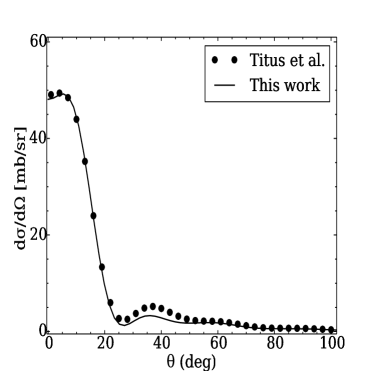
As mentioned before, the effect of non–local interactions in cross sections populating neutron bound states was studied in [1]. The present paper is an extension of this previous work to describe the population of neutron states in the continuum, but the formalism can also make predictions for bound states by considering solutions at negative neutron energy and taking to zero (see [2]). We use this fact to perform a benchmark of the new tools developed in the current study against those developed in [1, 28]. In Fig. 2 we show the angular distribution for the population of the ground state of 49Ca following with =20 MeV. We take the same parameters as [25]. Our results are shown with the solid line and agree well with those from Titus et al. [28]. Due to numerical difficulties associated with the iterative method implemented in [28], the corresponding calculation is not fully converged. This is the origin of the small discrepancies found around 40∘.
IV Predictions for the NEB cross sections
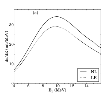
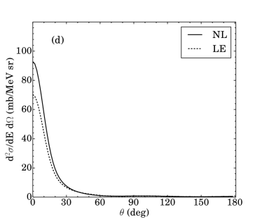
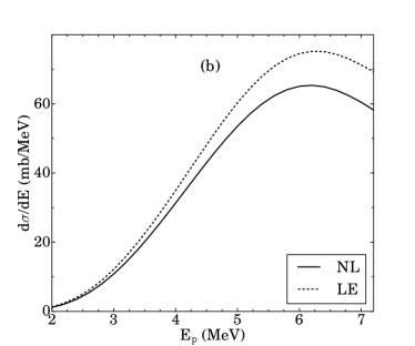
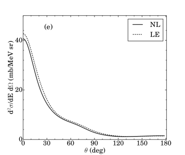
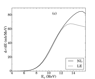
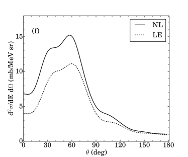
Given the strong interest in for surrogates, and the parallel between the NEB cross section and the transfer cross section to bound states [1], here we focus on the NEB contributions to the cross section. To illustrate the overall effect, we first show in Fig. 3 the energy and angular distributions for 16O at =20 MeV (panels a and d), 40Ca at =10 MeV (panels b and e), and 208Pb at =20 MeV (panels c and f). The plots show the predictions using the non–local interactions, labeled NL (solid lines), and those using the LEP, labeled LE (dotted lines). For all cases, the effects of nonlocality are significant. This overall conclusion is consistent with the studies for bound states [1]. However, given the complexity of the reaction theory, understanding the source for these large effects will prove to be more challenging than in [1].
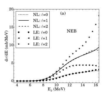
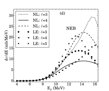
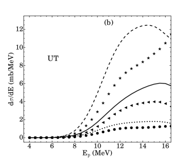
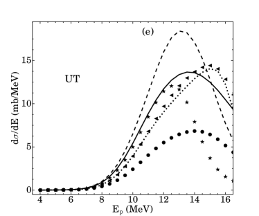
We next consider the contributions to the NEB, UT and HM terms from different partial waves (neutron–target angular momentum ). We remind here that in addition to the UT and HM term, there is also an interference term (see Eq. (1)). In Fig. 4, and for the 208Pb , =20 MeV reaction, we present the energy distributions for each partial wave () when using non–local interactions, and compare them with the corresponding results using LEPs. While for some partial waves, nonlocality has a negligible effect, for others the effect is very large and changes the shape of the distribution. Table 2 contains the partial wave contributions of the NEB cross section for 40Ca for =50 MeV at the peak of the energy distribution. We show results obtained with the LEPs (first row), followed by the percentage difference relative to the local, for the NEB cross sections at the peak of the energy distribution in three different situations: nonlocality is only included in (NL, second row), nonlocality is only included in (NL, third row) and nonlocality is included in both (NL, forth row). The proton energy at which these percentage differences are computed is also provided in the second column of Table 2. We see that for all partial waves, nonlocality in the proton channel reduces the cross section, while nonlocality in the neutron interaction can increase or decrease the cross sections. The competition between these two effects can result in either an increase or a decrease of the cross section.
| (MeV) | =0 | =1 | =2 | =3 | =4 | =5 | =6 | =7 | total (mb/MeV) | |
| LE (mb/MeV) | 26.1 | 0.36 | 1.13 | 2.16 | 2.70 | 5.03 | 5.49 | 2.06 | 0.65 | 19.58 |
| NL () | 26.8 | -11.11 | -14.20 | -10.70 | -10.00 | -8.80 | -12.60 | -15.53 | -16.92 | -11.54 |
| NL () | 27.2 | 30.56 | 6.20 | 31.02 | 24.8 | -3.20 | 23.90 | 42.72 | 27.69 | 19.05 |
| NL () | 27.4 | 33.33 | 0.02 | 29.63 | 18.15 | -10.14 | 16.76 | 31.55 | 12.31 | 12.21 |
| (MeV) | =0 | =1 | =2 | =3 | =4 | =5 | =6 | =7 | total (mb/MeV) | |
| LE (mb/MeV) | 26.1 | 0.18 | 0.46 | 0.96 | 1.55 | 1.62 | 1.55 | 0.55 | 0.09 | 6.96 |
| NL () | 26.8 | -22.20 | -23.90 | -21.90 | -17.40 | -23.50 | -32.90 | -42.27 | -44.44 | -26.15 |
| NL () | 27.2 | -2.20 | -2.20 | -12.50 | 27.10 | 21.60 | -0.70 | 0.00 | -3.33 | 8.95 |
| NL () | 27.4 | 0.01 | -4.35 | 4.17 | 74.19 | 50.01 | -6.45 | -25.45 | -22.22 | 24.71 |
| (MeV) | =0 | =1 | =2 | =3 | =4 | =5 | =6 | =7 | total (mb/MeV) | |
| LE (mb/MeV) | 26.1 | 0.24 | 0.73 | 1.61 | 3.06 | 3.37 | 3.18 | 2.12 | 0.84 | 15.15 |
| NL () | 26.8 | 2.51 | -6.85 | 4.35 | -3.92 | -2.37 | -2.20 | -14.62 | -23.81 | -4.98 |
| NL () | 27.2 | 58.99 | 56.16 | 68.94 | 59.15 | 51.04 | 43.71 | 32.08 | 20.24 | 49.05 |
| NL () | 27.4 | 58.33 | 42.47 | 20.19 | 50.00 | 47.18 | 39.94 | 15.09 | 0.01 | 41.52 |
| (MeV) | =0 | =1 | =2 | =3 | =4 | =5 | =6 | =7 | =8 | total (mb/MeV) | |
| LE (mb/MeV) | 13.6 | 2.34 | 4.44 | 9.19 | 13.86 | 10.00 | 20.01 | 3.64 | 2.62 | 1.37 | 67.47 |
| NL () | 15.0 | 16.67 | -0.90 | 31.96 | -10.46 | 41.00 | -34.98 | -21.43 | -16.03 | -19.71 | -4.13 |
| NL () | 15.5 | 19.23 | 94.37 | -5.88 | 111.98 | -13.70 | -1.50 | 0.55 | -4.58 | 25.55 | 26.47 |
| NL () | 14.7 | 13.68 | 83.33 | -13.06 | 85.43 | -9.00 | 11.44 | 25.27 | 3.05 | 31.39 | 25.92 |
| (MeV) | =0 | =1 | =2 | =3 | =4 | =5 | =6 | =7 | =8 | total (mb/MeV) | |
| LE (mb/MeV) | 13.6 | 1.11 | 3.76 | 8.09 | 6.76 | 13.15 | 9.75 | 1.36 | 1.15 | 0.33 | 45.46 |
| NL () | 15.0 | 1.80 | 4.26 | 13.10 | -6.36 | 9.66 | -62.46 | -2.21 | -21.74 | -27.27 | -9.63 |
| NL () | 15.5 | 49.55 | 43.62 | 42.03 | 96.75 | -17.57 | -1.33 | -44.12 | 36.52 | 121.21 | 21.73 |
| NL() | 14.7 | 63.64 | 54.79 | 53.89 | 105.30 | -1.75 | 46.77 | -32.35 | 55.65 | 127.27 | 42.15 |
| (MeV) | =0 | =1 | =2 | =3 | =4 | =5 | =6 | =7 | =8 | total (mb/MeV) | |
| LE (mb/MeV) | 13.6 | 1.44 | 5.11 | 8.46 | 10.05 | 8.14 | 5.26 | 2.88 | 1.30 | 0.66 | 43.30 |
| NL () | 15.0 | 11.11 | 2.54 | -3.78 | -6.77 | -14.74 | -9.70 | -20.49 | -15.38 | -13.64 | -7.62 |
| NL () | 15.5 | 75.69 | 56.56 | 42.08 | 33.63 | 16.95 | 23.57 | 5.21 | 10.77 | 15.15 | 32.17 |
| NL () | 14.7 | 72.92 | 60.27 | 51.30 | 44.18 | 31.20 | 34.41 | 17.01 | 21.54 | 21.21 | 41.96 |
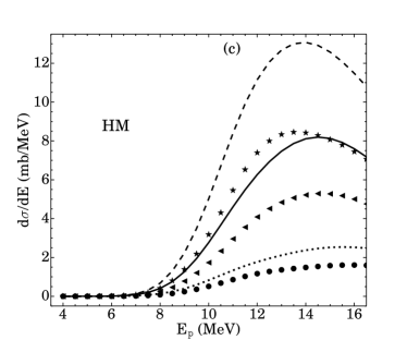
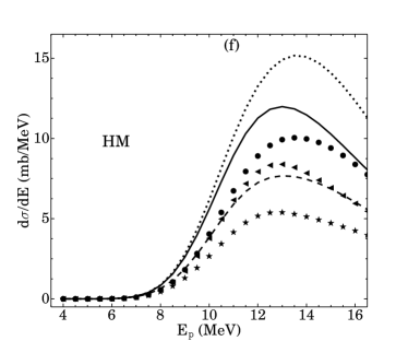
Given that there are three terms composing the total NEB cross section, and in each one of these, nonlocality enters differently (Eq. (1)), it is important to dissect further the results if we want to understand the origins of the overall effects shown in Fig. 3. In Table 2 we present the same partial wave contributions, either for the direct term (UT) or for the non–orthogonality term (HM). For UT, nonlocality in the proton wavefunction produces a strong reduction independently of the partial waves. The inclusion of nonlocality in is more complex, and varies considerably from % reduction to % increase. Most importantly, these effects interfere in such a way that even if both separate NL and NL show a decrease in the cross section, one can end up with a total effect that increases the cross section.
The HM term is somewhat simpler to analyse. Nonlocality in is not very strong, the effects are dominated by the difference in the actual interactions since is different for the LEP and the non–local Perey and Buck interaction (see also Fig. 10).
Moreover, we should note that the effects of nonlocality depend strongly on the reaction studied. As an illustration of this fact, Table 3 contains the same information as Table 2 but now for the reaction 208Pb at 20.0 MeV. The magnitudes and the signs of the percentage differences can change considerably, indicating a complex balance between the various ingredients, and a strongly non-linear effect.
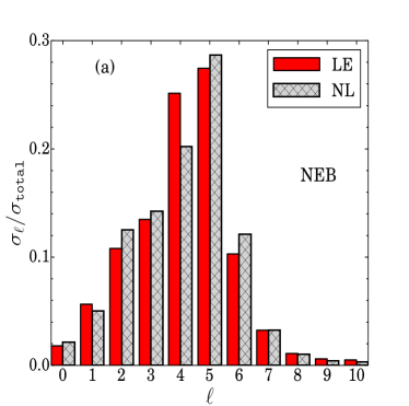
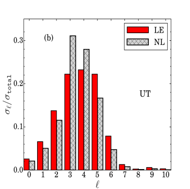
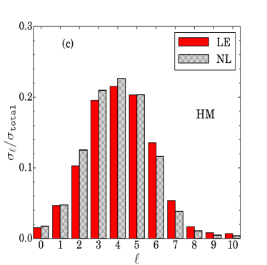
Finally, and keeping in mind that the most important input of this reaction theory for the surrogate method is the cross section distribution as a function of the neutron-target partial wave (so-called spin distributions), we show in Fig. 5 the histograms for the ratio of the cross section corresponding to each neutron partial wave over the total cross section, as a function of , for the results obtained with either the LEPs (red, plain) and the non–local interactions (grey, hatched). In Fig. 5a, we show the NEB cross section while in Fig. 5b (c) we show the UT (HM) contribution. The spin distributions shown in Fig. 5 refer to the reaction 40Ca at 50 MeV.
As we had seen before, nonlocality has a sizable effect in the overall magnitude of the cross section. However, the relative importance of the different values is mostly unchanged. As a consequence, the angular differential cross section conserves its shape when including non–local interactions as demonstrated by Figs. 3 (d), (e), (f).
V Understanding the effects of nonlocality
So far we have shown that nonlocality has large effects on the NEB cross sections, however it is not easy to interpret those effects in terms of specific physical features of the system. To get a better understanding of the effects of nonlocality, we now turn to the essential ingredients that drive the effects we are seeing, namely the sources and the actual interactions. Because the various terms in the NEB cross section relate directly to matrix elements of , the relevant region of space to consider is the surface region.
We first look at the proton vertex functions, which correspond to the source in the equation for calculating the proton distorted waves (see Eq. (8)). The expressions for the local and non–local proton vertex for a specific functions are given by:
| (24) |
In Fig. 6, we compare the non–local (solid line) with the local vertex functions defined in Eq. (V) for + 40Ca (panel a) and +208Pb (panel b), in both cases for . Consistently with previous studies, it is observed that the NL vertex function is reduced in the interior region, and enhanced in the exterior, with respect to the local result.
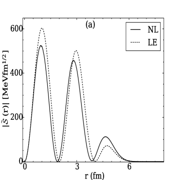
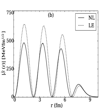
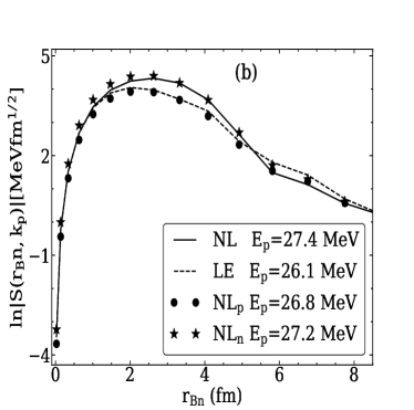
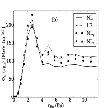
We next consider the two elements needed to calculate the neutron wavefunction , namely the source defined in Eq. (6) and the Green’s function . In Fig. 7 we show the source term for 40Ca at =20 MeV (panel a) and =50 MeV (panel b). Again the results are shown for the case in which we include nonlocality in both the neutron and proton interactions (NL, solid line) and compare to those using the LEPs (LE, dotted line). We also show the result when including nonlocality only in (NL, circles) or only in (NL, stars). The calculations are performed at the proton energy corresponding to the peak of the NEB energy differential cross section, i.e. =27.4 MeV for NL, =27.2 MeV for NL, =26.8 MeV for NL, and =26.1 MeV for LE. Nonlocality in the neutron interaction has the effect of increasing the source term in the nuclear interior (comparing LE with NL), while nonlocality in the proton interaction causes a more modest reduction of the source term in the internal region (comparing LE with NL).
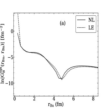
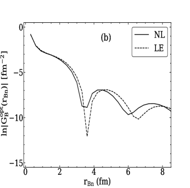
In Fig. 8 we show the diagonal part of the Green’s functions for + 40Ca; =6.74 MeV for LE (6.37 MeV for NL), =3 and =7/2 (panel a) and + 40Ca; =20.43 MeV for LE (19.13 MeV for NL), =2 and =5/2 (panel b) . We show the results obtained including nonlocality in (NL, solid line) and those obtained using the corresponding LEP (LE, dotted line). It can be seen that nonlocality reduces the diagonal part of the Green’s function in the internal region with respect to the LE calculation, and shifts the function at larger distances.
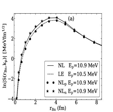
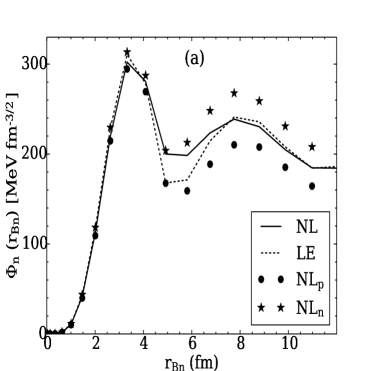
The neutron wavefunction in the field of the target following the breakup of the deuteron is a product of the source and the Green’s function (Eq. (5)). The results corresponding to the cases considered in Figs. 7 and 8 are displayed in Fig. 9. By comparing the results with local interactions (dotted line) with those using non–local interactions (solid line) we find that overall nonlocality reduces the wavefunction in the interior but its effect in the exterior region depends on the beam energy, caused by the radial shift in the Green’s function shown in Fig. 8. Fig. 9 also shows that nonlocality in and have opposite effects: while the neutron wavefunction obtained including nonlocality in only (NL, stars) is larger than the local counterpart (LE), the neutron wavefunction obtained including nonlocality in only (NL, circles) is smaller than the local one.
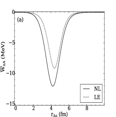
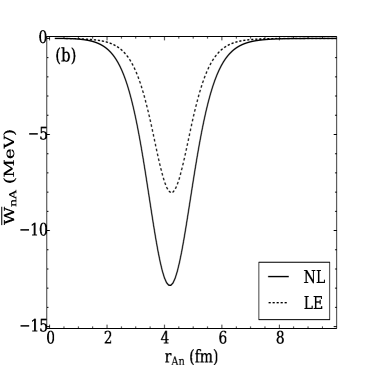
Finally, we look at the imaginary term . In order to be able to compare the non–local potential with the local equivalent (Table 1), we plot the non–local neutron potential after integration over one of the radial variables . We pick the same cases relevant to the examples shown in Fig. 7. In Fig. 10 we show the imaginary potential for the 40Ca+ system for: =6.34 MeV (panel a) and =19.13 MeV (panel b) (these energies correspond to the neutron energies at the peak of the NEB energy distribution for at 20 MeV and 50 MeV respectively). It is apparent that the absolute value of the imaginary term of the non–local potential is larger than the one of the corresponding local equivalent.
By inspecting the various ingredients of the reaction theory, we are now able to justify the varied effects that nonlocality can have on the NEB cross sections. The overall reduction of the neutron wavefunction in the interior competes with the increase of the magnitude of the non–local interaction to produce the complex effects on the cross sections discussed in Section IV.
VI Conclusion
In this work, we explore the effects of nonlocality in reactions populating continuum states in the final nucleus within the model described in [2]. This study is an extension of the study done in [1] for to bound states.
This is a systematic study: we include reactions on 16O, 40Ca, 48Ca and 208Pb at varies beam energies =10 MeV, 20 MeV and 50 MeV. We analyse energy distributions, angular distributions as well as spin distributions. We compare results obtained using non–local and interactions, with those obtained using the corresponding local equivalent potentials.
Our results demonstrate that the importance of the effect of nonlocality on the magnitude and the shape of the distributions is dependent on beam energy, target, and final spin state. Overall, we find that nonlocality has a non-negligible effect on the non-elastic breakup cross sections, the component that is relevant to the surrogate method and to the extraction of the neutron capture cross section. The effect can be as large as 85% in some cases, especially for heavier targets.
Understanding the specific origins of the overall effect on the cross sections is not easy, due to the complexity of the reaction theory used to describe these inclusive processes. Nonlocality acts in such a way that it produces a reduction in the interior of the neutron wavefunction in the field of the target, following the breakup. At the same time, the imaginary term of the neutron optical potential, responsible for the capture of the neutron into the final state increases in absolute value. These two effects compete and can produce large variations on the resulting cross section, including both enhancements and reductions.
Nevertheless, and even if the magnitude of the cross sections can change considerably, the relative weights of the various spin contributions are mostly unaltered with nonlocality. Since this is the most important input to the surrogate method analysis, it is reassuring that previous studies will not be brought into question with the results presented here [10, 11, 2].
Acknowledgement
We gratefully acknowledge I. J. Thompson for useful discussions and comments. This work was supported by the National Science Foundation under Grant PHY-1520929, the U.S. Department of Energy National Nuclear Security Administration under the Stewardship Science Academic Alliances program, NNSA Grant No. DE-NA0000979 and No. DE-FG52- 08NA28552.
References
- [1] L. J. Titus and F. M. Nunes. Testing the Perey effect. Phys. Rev. C, 89:034609, Mar 2014.
- [2] G. Potel, F. M. Nunes, and I. J. Thompson. Establishing a theory for deuteron-induced surrogate reactions. Phys. Rev. C, 92:034611, Sep 2015.
- [3] A Spyrou, A C Larsen, S N Liddick, F Naqvi, B P Crider, A C Dombos, M Guttormsen, D L Bleuel, A Couture, L Crespo Campo, R Lewis, S Mosby, M R Mumpower, G Perdikakis, C J Prokop, S J Quinn, T Renstrøm, S Siem, and R Surman. Neutron-capture rates for explosive nucleosynthesis: the case of . Journal of Physics G: Nuclear and Particle Physics, 44(4):044002, 2017.
- [4] M.R. Mumpower, R. Surman, G.C. McLaughlin, and A. Aprahamian. The impact of individual nuclear properties on r-process nucleosynthesis. Progress in Particle and Nuclear Physics, 86:86 – 126, 2016.
- [5] J.A. Cizewski, R. Hatarik, K.L. Jones, S.D. Pain, J.S. Thomas, M.S. Johnson, D.W. Bardayan, J.C. Blackmon, M.S. Smith, and R.L. Kozub. reactions and the surrogate reaction technique. Nuclear Instruments and Methods in Physics Research Section B: Beam Interactions with Materials and Atoms, 261(1):938 – 940, 2007. The Application of Accelerators in Research and Industry.
- [6] Cizewski, Jolie A., Ratkiewicz, Andrew, Escher, Jutta E., Lepailleur, Alexandre, Pain, Steven D., and Potel, Gregory. Informing neutron capture nucleosynthesis on short-lived nuclei with reactions. EPJ Web Conf., 165:01013, 2017.
- [7] B V Carlson, R Capote, and M Sin. Elastic and inelastic breakup of deuterons with energy below 100 MeV. 2015.
- [8] Jin Lei and Antonio M. Moro. Numerical assessment of post-prior equivalence for inclusive breakup reactions. Phys. Rev. C, 92:061602, Dec 2015.
- [9] Jin Lei and A. M. Moro. Reexamining closed-form formulae for inclusive breakup: Application to deuteron- and -induced reactions. Phys. Rev. C, 92:044616, Oct 2015.
- [10] G. Potel, G. Perdikakis, B. V. Carlson, M. C. Atkinson, W. H. Dickhoff, J. E. Escher, M. S. Hussein, J. Lei, W. Li, A. O. Macchiavelli, A. M. Moro, F. M. Nunes, S. D. Pain, and J. Rotureau. Toward a complete theory for predicting inclusive deuteron breakup away from stability. The European Physical Journal A, 53(9):178, Sep 2017.
- [11] A. Ratkiewicz, J.A. Cizewski, J.E. Escher, G. Potel, J.T. Burke, R.J. Casperson, M. McCleskey, R.A.E. Austin, S. Burcher, R.O. Hughes, B. Manning, S.D. Pain, W.A. Peters, S. Rice, T.J. Ross, N.D. Scielzo, C. Shand, and K. Smith. Neutron capture on exotic nuclei: Demonstrating the reaction as a for . submitted to Phys. Rev. Lett.
- [12] L. Canton, G. Pisent, J. P. Svenne, D. van der Knijff, K. Amos, and S. Karataglidis. Role of the Pauli principle in collective-model coupled-channel calculations. Phys. Rev. Lett., 94:122503, Apr 2005.
- [13] P. Fraser, K. Amos, S. Karataglidis, L. Canton, G. Pisent, and J. P. Svenne. Two causes of nonlocalities in nucleon-nucleus potentials and their effects in nucleon-nucleus scattering. The European Physical Journal A, 35(1):69–80, Jan 2008.
- [14] G. H. Rawitscher, D. Lukaszek, R. S. Mackintosh, and S. G. Cooper. Local representation of the exchange nonlocality in n O scattering. Phys. Rev. C, 49:1621–1629, Mar 1994.
- [15] Herman Feshbach. Unified theory of nuclear reactions. Ann. Phys., 5(4):357 – 390, 1958.
- [16] Herman Feshbach. A unified theory of nuclear reactions. II. Ann. Phys., 19(2):287 – 313, 1962.
- [17] C. Mahaux and R. Sartor. Single-Particle Motion in Nuclei, pages 1–223. Springer US, Boston, MA, 1991.
- [18] M. H. Mahzoon, R. J. Charity, W. H. Dickhoff, H. Dussan, and S. J. Waldecker. Forging the link between nuclear reactions and nuclear structure. Phys. Rev. Lett., 112:162503, Apr 2014.
- [19] J. Rotureau, P. Danielewicz, G. Hagen, F. M. Nunes, and T. Papenbrock. Optical potential from first principles. Phys. Rev. C, 95:024315, Feb 2017.
- [20] N. Austern. Wave functions of nonlocal potentials: The perey effect. Phys. Rev., 137:B752–B757, Feb 1965.
- [21] Norman Austern. Direct nuclear reaction theories. New York : Wiley-Interscience, 1970.
- [22] H. Fiedeldey. The equivalent local potential and the perey effect. Nucl. Phys., 77(1):149 – 156, 1966.
- [23] M. Igarashi, M. Toyama, and N. Kishida. Computer Program TWOFNR.
- [24] P.D. Kunz. Instructions for the use of dwuck: A distorted wave born approximation program.
- [25] L. J. Titus, F. M. Nunes, and G. Potel. Explicit inclusion of nonlocality in transfer reactions. Phys. Rev. C, 93:014604, Jan 2016.
- [26] F. Perey and B. Buck. A non-local potential model for the scattering of neutrons by nuclei. Nuclear Physics, 32:353 – 380, 1962.
- [27] A. E. Lovell, P.-L. Bacq, P. Capel, F. M. Nunes, and L. J. Titus. Energy dependence of nonlocal optical potentials. Phys. Rev. C, 96:051601, Nov 2017.
- [28] L.J. Titus, A. Ross, and F.M. Nunes. Transfer reaction code with nonlocal interactions. Computer Physics Communications, 207:499 – 517, 2016.
- [29] P Descouvemont and D Baye. The R-matrix theory. Reports on Progress in Physics, 73(3):036301, 2010.
- [30] J. Bonitati. Report from research experience for undergraduates. private communication, 2017.
- [31] T. Udagawa and T. Tamura. Breakup-fusion description of massive transfer reactions with emission of fast light particles. Phys. Rev. Lett., 45:1311–1314, Oct 1980.
- [32] M.S. Hussein and K.W. McVoy. Inclusive projectile fragmentation in the spectator model. Nuclear Physics A, 445(1):124 – 139, 1985.
- [33] Weichuan Li, G. Potel, F.M. Nunes, and I.J. Thompson. A method for solving the Dyson equation with non-local interactions. in preparation.
- [34] Eugene P. Wigner. Resonance reactions. Phys. Rev., 70:606–618, Nov 1946.
- [35] A. M. Lane and R. G. Thomas. R-matrix theory of nuclear reactions. Rev. Mod. Phys., 30:257–353, Apr 1958.
- [36] D Baye, M Hesse, J-M Sparenberg, and M Vincke. Analysis of the R-matrix method on Lagrange meshes. Journal of Physics B: Atomic, Molecular and Optical Physics, 31(15):3439, 1998.
- [37] John C. Light and Robert B. Walker. An R matrix approach to the solution of coupled equations for atommolecule reactive scattering. The Journal of Chemical Physics, 65(10):4272–4282, 1976.
- [38] Yinlu Han, Yuyang Shi, and Qingbiao Shen. Deuteron global optical model potential for energies up to 200 mev. Phys. Rev. C, 74:044615, 2006.
- [39] Ian J. Thompson. Coupled reaction channels calculations in nuclear physics. Comput. Phys. Rept., 7:167–212, 1988.