Tight Dimension Independent Lower Bound on the Expected Convergence Rate for Diminishing Step Sizes in SGD

Abstract

We study the convergence of Stochastic Gradient Descent (SGD) for strongly convex objective functions. We prove for all $t$ a lower bound on the expected convergence rate after the $t$-th SGD iteration; the lower bound is over all possible sequences of diminishing step sizes. It implies that recently proposed sequences of step sizes at ICML 2018 and ICML 2019 are universally close to optimal in that the expected convergence rate after each iteration is within a factor $32$ of our lower bound. This factor is independent of dimension $d$. We offer a framework for comparing with lower bounds in state-of-the-art literature and when applied to SGD for strongly convex objective functions our lower bound is a significant factor $775\cdot d$ larger compared to existing work.

1 Introduction

We are interested in solving the following stochastic optimization problem

$$\min_{w\in\mathbb{R}^{d}}\left\{F(w)=\mathbb{E}[f(w;\xi)]\right\},$$ (1)

where $\xi$ is a random variable obeying some distribution $g(\xi)$. In the case of empirical risk minimization with a training set $\{(x_{i},y_{i})\}_{i=1}^{n}$, $\xi_{i}$ is a random variable that is defined by a single random sample $(x,y)$ pulled uniformly from the training set. Then, by defining $f_{i}(w):=f(w;\xi_{i})$, empirical risk minimization reduces to

$$\min_{w\in\mathbb{R}^{d}}\left\{F(w)=\frac{1}{n}\sum_{i=1}^{n}f_{i}(w)\right\}.$$ (2)

Problems of this type arise frequently in supervised learning applications Hastie et al. (2009). The classic first-order methods to solve problem (2) are gradient descent (GD) Nocedal and Wright (2006) and stochastic gradient descent (SGD) Robbins and Monro (1951) algorithms. GD is a standard deterministic gradient method, which updates iterates along the negative full gradient with learning rate $\eta_{t}$ as follows

$$w_{t+1}=w_{t}-\eta_{t}\nabla F(w_{t})=w_{t}-\frac{\eta_{t}}{n}\sum_{i=1}^{n}\nabla f_{i}(w_{t})\ ,\ t\geq 0.$$

We can choose $\eta_{t}=\eta=\operatorname{\mathcal{O}}(1/L)$ and achieve a linear convergence rate for the strongly convex case Nesterov (2004). The upper bound of the convergence rate of GD and SGD has been studied in  Bertsekas (1999); Boyd and Vandenberghe (2004); Nesterov (2004); Schmidt and Roux (2013); Nguyen et al. (2018b, a); Gower et al. (2019).

The disadvantage of GD is that it requires evaluation of $n$ derivatives at each step, which is very expensive and therefore avoided in large-scale optimization. To reduce the computational cost for solving (2), a class of variance reduction methods Le Roux et al. (2012); Defazio et al. (2014); Johnson and Zhang (2013); Nguyen et al. (2017) has been proposed. The difference between GD and variance reduction methods is that GD needs to compute the full gradient at each step, while the variance reduction methods will compute the full gradient after a certain number of steps. In this way, variance reduction methods have less computational cost compared to GD. To avoid evaluating the full gradient at all, SGD generates an unbiased random variable $\xi_{t}$ satisfying

$$\mathbb{E}_{\xi_{t}}[\nabla f(w_{t};\xi_{t})]=\nabla F(w_{t}),$$

and then evaluates gradient $\nabla f(w_{t};\xi_{t})$ for $\xi_{t}$ drawn from a distribution $g(\xi)$. After this, $w_{t}$ is updated as follows

$$w_{t+1}=w_{t}-\eta_{t}\nabla f(w_{t};\xi_{t}).$$ (3)

We focus on the general problem (1) where $F$ is strongly convex. Since $F$ is strongly convex, a unique optimal solution of (1) exists and throughout the paper we denote this optimal solution by $w_{*}$ and are interested in studying the expected convergence rate

$$Y_{t}=\mathbb{E}[\|w_{t}-w_{*}\|^{2}].$$

Algorithm 1 provides a detailed description of SGD. Obviously, the computational cost of a single iteration in SGD is $n$ times cheaper than that of a single iteration in GD. However, as has been shown in literature we need to choose $\eta_{t}=\operatorname{\mathcal{O}}(1/t)$ and the expected convergence rate of SGD is slowed down to $\operatorname{\mathcal{O}}(1/t)$ Bottou et al. (2016), which is a sublinear convergence rate.

Algorithm 1 Stochastic Gradient Descent (SGD) Method

  Initialize: $w_{0}$

  Iterate:

  for $t=0,1,\dots$ do

     Choose a step size (i.e., learning rate) $\eta_{t}>0$.

     Generate a random variable $\xi_{t}$ with probability density $g(\xi_{t})$.

     Compute a stochastic gradient $\nabla f(w_{t};\xi_{t}).$

     Update the new iterate $w_{t+1}=w_{t}-\eta_{t}\nabla f(w_{t};\xi_{t})$.

  end for

Problem Statement and Contributions: We seek to find a tight lower bound on the expected convergence rate $Y_{t}$ with the purpose of showing that the stepsize sequences of Nguyen et al. (2018b) and Gower et al. (2019) for classical SGD is optimal for $\mu$-strongly convex and $L$-smooth respectively expected $L$-smooth objective functions within a small dimension independent constant factor. This is important because of the following reasons:

1. The lower bound tells us that a sequence of stepsizes as a function of only $\mu$ and $L$ cannot beat an expected convergence rate of $O(1/t)$ – this is known general knowledge and was already proven in Agarwal et al. (2009), where a dimension dependent lower bound for a larger class of algorithms that includes SGD was proven. For the class of SGD with diminishing stepsizes as a function of only global parameters $\mu$ and $L$ we show a dimension independent lower bound which is a factor $775\cdot d$ larger.

2. We now understand into what extent the sequence of stepsizes of Nguyen et al. (2018b) and Gower et al. (2019) are optimal in that it leads to minimal expected convergence rates $Y_{t}$ for all $t$: For each $t$ we will show a dimension independent lower bound on $Y_{t}$ over all possible stepsize sequences. This includes the best possible stepsize sequence which minimizes $Y_{t}$ for a given $t$. Our lower bound achieves the upper bound on $Y_{t}$ for the stepsize sequences of Nguyen et al. (2018b) and Gower et al. (2019) within a factor 32 for all $t$. This implies that these stepsize sequences universally minimizes each $Y_{t}$ within factor 32.

3. As a consequence, in order to attain a better expected convergence rate, we need to either assume more specific knowledge about the objective function $F$ so that we can construct a better stepsize sequence for SGD based on this additional knowledge or we need to step away from SGD and use a different kind of algorithm. For example, the larger class of algorithms in Agarwal et al. (2009) may contain a non-SGD algorithm which may get close to the lower bound proved in Agarwal et al. (2009) which is a factor $775\cdot d$ smaller. Since the larger class of algorithms in  Agarwal et al. (2009) contains algorithms such as Adam Kingma and Ba (2014), AdaGrad Duchi et al. (2011), SGD-Momentum Sutskever et al. (2013), RMSProp Zou et al. (2018) we now know that these practical algorithms will at most improve a factor $32\cdot 775\cdot d$ over SGD for strongly convex optimization – this can be significant as this can lead to orders of magnitude less gradient computations. We are the first to make such quantification.

Outline: Section 2 discusses background: First, we discuss the recurrence on $Y_{t}$ used in Nguyen et al. (2018b) for proving their upper bound on $Y_{t}$ – this recurrence plays a central role in proving our lower bound. We discuss the upper bounds of both Nguyen et al. (2018b) and Gower et al. (2019) – the latter holding for a larger class of algorithms. Second, we explain the lower bound of  Agarwal et al. (2009) in detail in order to be able to properly compare with our lower bound. Section 3 introduces a framework for comparing bounds and explains the consequences of our lower bound in detail. Section 4 describes a class of strongly convex and smooth objective functions which is used to derive our lower bound. We also verify our theory by experiments in the supplementary material. Section 5 concludes the paper.

2 Background

We explain the upper bound of Nguyen et al. (2018b); Gower et al. (2019), and lower bound of Agarwal et al. (2009) respectively.

2.1 Upper Bound for Strongly Convex and Smooth Objective Functions

The starting point for analysis is the recurrence first introduced in Nguyen et al. (2018b); Leblond et al. (2018)

$$\mathbb{E}[\|w_{t+1}-w_{*}\|^{2}]\leq(1-\mu\eta_{t})\mathbb{E}[\|w_{t}-w_{*}\|^{2}]+\eta_{t}^{2}N,$$ (4)

where

$$N=2\mathbb{E}[\|\nabla f(w_{*};\xi)\|^{2}]$$

and $\eta_{t}$ is upper bounded by $\frac{1}{2L}$; the recurrence has been shown to hold, see Nguyen et al. (2018b); Leblond et al. (2018), if we assume

1. $F(.)$ is $\mu$-strongly convex,

2. $f(w;\xi)$ is $L$-smooth,

3. $f(w;\xi)$ is convex, and

4. $N$ is finite;

we detail these assumptions below:

Assumption 1 ($\mu$-strongly convex).

The objective function $F:\mathbb{R}^{d}\to\mathbb{R}$ is $\mu$-strongly convex, i.e., there exists a constant $\mu>0$ such that $\forall w,w^{\prime}\in\mathbb{R}^{d}$,

$$F(w)-F(w^{\prime})\geq\langle\nabla F(w^{\prime}),(w-w^{\prime})\rangle+\frac{\mu}{2}\|w-w^{\prime}\|^{2}.$$ (5)

Assumption 2 ($L$-smooth).

$f(w;\xi)$ is $L$-smooth for every realization of $\xi$, i.e., there exists a constant $L>0$ such that, $\forall w,w^{\prime}\in\mathbb{R}^{d}$,

$$\|\nabla f(w;\xi)-\nabla f(w^{\prime};\xi)\|\leq L\|w-w^{\prime}\|.$$ (6)

Assumption 2 implies that $F$ is also $L$-smooth.

Assumption 3.

$f(w;\xi)$ is convex for every realization of $\xi$, i.e., $\forall w,w^{\prime}\in\mathbb{R}^{d}$,

$$f(w;\xi)-f(w^{\prime};\xi)\geq\langle\nabla f(w^{\prime};\xi),(w-w^{\prime})\rangle.$$

Assumption 4.

$N=2\mathbb{E}[\|\nabla f(w_{*};\xi)\|^{2}]$ is finite.

We denote the set of strongly convex objective functions by ${\cal F}_{str}$ and denote the subset of ${\cal F}_{str}$ satisfying Assumptions 1, 2, 3, and 4 by ${\cal F}_{sm}$.

We notice that the earlier established recurrence in Moulines and Bach (2011) under the same set of assumptions

$$\mathbb{E}[\|w_{t+1}-w_{*}\|^{2}] \leq(1-2\mu\eta_{t}+2L^{2}\eta_{t}^{2})\mathbb{E}[\|w_{t}-w_{*}\|^{2}]+\eta_{t}^{2}N$$

is similar, but worse than (4) as it only holds for $\eta_{t}<\frac{\mu}{L^{2}}$ where (4) holds for $\eta_{t}\leq\frac{1}{2L}$. Only for step sizes $\eta_{t}<\frac{\mu}{2L^{2}}$ the above recurrence provides a better bound than (4), i.e., $1-2\mu\eta_{t}+2L^{2}\eta_{t}^{2}\leq 1-\mu\eta_{t}$. In practical settings such as logistic regression $\mu=\operatorname{\mathcal{O}}(1/n)$, $L=\operatorname{\mathcal{O}}(1)$, and $t=\operatorname{\mathcal{O}}(n)$ (i.e. $t$ is at most a relatively small constant number of epochs, where a single epoch represents $n$ iterations resembling the complexity of a single GD computation). See (8) below, for this parameter setting the optimally chosen step sizes are $\gg\frac{\mu}{L^{2}}$. This is the reason we focus in this paper on analyzing recurrence (4) in order to prove our lower bound: For $\eta_{t}\leq\frac{1}{2L}$,

$$\hskip 8.53581ptY_{t+1}\leq(1-\mu\eta_{t})Y_{t}+\eta_{t}^{2}N,$$ (7)

where $Y_{t}=\mathbb{E}[\|w_{t}-w_{*}\|^{2}]$.

Based on the above assumptions (without the so-called bounded gradient assumption) and knowledge of only $\mu$ and $L$ a sequence of step sizes $\eta_{t}$ can be constructed such that $Y_{t}$ is smaller than $\operatorname{\mathcal{O}}(1/t)$ Nguyen et al. (2018b); more explicitly, for the sequence of step sizes

$$\eta_{t}=\frac{2}{\mu t+4L}$$ (8)

we have for all objective functions in ${\cal F}_{sm}$ the upper bound

$$Y_{t}\leq\frac{16N}{\mu}\frac{1}{\mu(t-T^{\prime})+4L}=\frac{16N}{\mu^{2}t}(1+{\cal O}(1/t)),$$ (9)

where

$$t\geq T^{\prime}=\frac{4L}{\mu}\max\{\frac{L\mu Y_{0}}{N},1\}-\frac{4L}{\mu}.$$

We notice that  Gower et al. (2019) studies the larger class, which we denote ${\cal F}_{esm}$, which is defined as ${\cal F}_{sm}$ where expected smoothness is assumed in stead of smoothness and convexity of component functions. We rephrase their assumption for classical SGD as studied in this paper.

Assumption 5.

($L$-smooth in expectation) The objective function $F:\mathbb{R}^{d}\to\mathbb{R}$ is $L$-smooth in expectation if there exists a constant $L>0$ such that, $\forall w\in\mathbb{R}^{d}$,

$$\mathbb{E}[\|\nabla f(w;\xi)-\nabla f(w_{*};\xi)\|^{2}]\leq 2L\|F(w)-F(w_{*})\|.$$ (10)

The results in Gower et al. (2019) assume the above assumption for empirical risk minimization (2). $L$-smoothness, see Nesterov (2004), implies Lipschitz continuity (i.e., $\forall w,w^{\prime}\in\mathbb{R}^{d}$,

$$f(w,\xi)\leq f(w^{\prime},\xi)+\langle\nabla f(w^{\prime},\xi),(w-w^{\prime})\rangle+\frac{L}{2}\|w-w^{\prime}\|^{2}$$

) and together with Proposition A.1 in Gower et al. (2019) this implies $L$-smooth in expectation. This shows that ${\cal F}_{esm}$ defined by Assumptions 1, 4, and 5 is indeed a superset of ${\cal F}_{sm}$.

The step sizes (8) from Nguyen et al. (2018b) for ${\cal F}_{sm}\subseteq{\cal F}_{esm}$ and

$$\eta_{t}=\frac{2t+1}{(t+1)^{2}\mu}\mbox{ for }t>\frac{4L}{\mu}\mbox{ and }\eta_{t}=\frac{1}{2L}\mbox{ for }t\leq\frac{4L}{\mu}$$ (11)

developed for ${\cal F}_{esm}$ in Gower et al. (2019) and  Nguyen et al. (2018b) are equivalent in that they are both $\approx\frac{2}{\mu t}$ for $t$ large enough. Both step size sequences give exactly the same asymptotic upper bound (9) on $Y_{t}$ (in our notation).

In Robbins and Monro (1951), the authors proved the convergence of SGD for the step size sequence $\{\eta_{t}\}$ satisfying conditions $\sum_{t=0}^{\infty}\eta_{t}=\infty\ \text{and}\ \sum_{t=0}^{\infty}\eta_{t}^{2}<\infty$. In Moulines and Bach (2011), the authors studied the expected convergence rates for another class of step sizes of $\mathcal{O}(1/t^{p})$ where $0<p\leq 1$. However, the authors of both Robbins and Monro (1951) and Moulines and Bach (2011) do not discuss about the optimal step sizes among all proposed step sizes which is what is done in this paper.

2.2 Lower Bound for First Order Stochastic Oracles

The authors of Nemirovsky A.S. and IUdin (c1983.) proposed the first formal study on lower bounding the expected convergence rate for a large class of algorithms which includes SGD. The authors of Agarwal et al. (2009) and Raginsky and Rakhlin (2011) independently studied this lower bound using information theory and were able to improve it.

The derivation in Agarwal et al. (2009) is for algorithms including SGD where the sequence of stepsizes is a-priori fixed based on global information regarding assumed stochastic parameters concerning the objective function $F$. Their proof uses the following set of assumptions: First, The assumption of a strongly convex objective function, i.e., Assumption 1 (see Definition 3 in Agarwal et al. (2009)). Second, the objective function is convex Lipschitz:

Assumption 6.

(convex Lipschitz) The objective function $F$ is a convex Lipschitz function, i.e., there exists a bounded convex set $\mathcal{S}\subset\mathbb{R}^{d}$ and a positive number $K$ such that $\forall w,w^{\prime}\in\mathcal{S}\subset\mathbb{R}^{d}$

$$\|F(w)-F(w^{\prime})\|\leq K\|w-w^{\prime}\|.$$

We notice that this assumption implies the assumption on bounded gradients as stated here (and explicitly mentioned in Definition 1 in Agarwal et al. (2009)): There exists a bounded convex set $\mathcal{S}\subset\mathbb{R}^{d}$ and a positive number $\sigma$ such that

$$\mathbb{E}[\|\nabla f(w;\xi)\|^{2}]\leq\sigma^{2}$$ (12)

for all $w\in\mathcal{S}\subset\mathbb{R}^{d}$. This is not the same as the bounded gradient assumption where $\mathcal{S}=\mathbb{R}^{d}$ is unbounded. Clearly, for $w_{*}$, (12) implies a finite $N\leq 2\sigma^{2}$.

We define ${\cal F}_{lip}$ as the set of strongly convex objective functions that satisfy Assumption 6. Classes ${\cal F}_{esm}$ and ${\cal F}_{lip}$ are both subsets of ${\cal F}_{str}$ and differ (are not subclasses of each other) in that they assume expected smoothness and convex Lipschitz respectively.

To prove a lower bound of $Y_{t}$ for ${\cal F}_{lip}$, the authors constructed a class of objective functions $\subseteq{\cal F}_{lip}$ and showed a lower bound of $Y_{t}$ for this class; in terms of the notation used in this paper,

$$\frac{\log(2/\sqrt{e})}{432\cdot d}\frac{N}{\mu^{2}t}.$$ (13)

The authors of Agarwal et al. (2009) prove lower bound (13) for the class ${\cal A}_{stoch}$ of stochastic first order algorithms that can be understood as operating based on information provided by a stochastic first-order oracle, i.e., any algorithm which bases its computation in the $t$-th iteration on $\mu$, $K$ or $L$, $d$, and access to an oracle that provides $f(w_{t};\xi_{t})$ and $\nabla f(w_{t};\xi_{t})$. This class includes ${\cal A}_{SGD}$ defined as SGD with some sequence of diminishing step sizes as a function of global parameters such as $\mu$ and $L$ or $\mu$ and $K$, see Algorithm 1. We notice that ${\cal A}_{stoch}$ also includes practical algorithms such as Adam Kingma and Ba (2014), etc. We revisit their derivation in the supplementary material where we show how their lower bound transforms into (13). Notice that their lower bound depends on dimension $d$.

3 Framework for Upper and Lower Bounds

Let $par(F)$ denote the concrete values of the global parameters of an objective function $F$ such as the values for $\mu$ and $L$ corresponding to objective functions $F$ in ${\cal F}_{sm}$ and ${\cal F}_{esm}$ or $\mu$ and $K$ corresponding to objective functions $F$ in ${\cal F}_{lip}$. When defining a class ${\cal F}$ of objective functions, we also need to explain how ${\cal F}$ defines a corresponding $par(.)$ function. We will use the notation ${\cal F}[p]$ to stand for the subclass $\{F\in{\cal F}\ :\ p=par(F)\}\subseteq{\cal F}$, i.e., the subclass of objective functions of ${\cal F}$ with the same parameters $p$. We assume that parameters of a class are included in the parameters of a smaller subclass: For example, ${\cal F}_{sm}$ is a subset of the class of strongly convex objective functions ${\cal F}_{str}$ with only global parameter $\mu$. This means that for concrete values $\mu$ and $L$ we have ${\cal F}_{sm}[\mu,L]\subseteq{\cal F}_{str}[\mu]$.

For a given objective function $F$, we are interested in the best possible expected convergence rate after the $t$-th iteration among all possible algorithms $A$ in a larger class of algorithms ${\cal A}$. Here, we assume that ${\cal A}$ is a subclass of the larger class ${\cal A}_{stoch,{\cal U}}$ of stochastic first order algorithms where the computation in the $t$-th iteration not only has access to $par(F)$ and access to an oracle that provides $f(w_{t};\xi_{t})$ and $\nabla f(w_{t};\xi_{t})$ but also access to possibly another oracle ${\cal U}$ providing even more information. Notice that ${\cal A}\subseteq{\cal A}_{stoch}\subseteq{\cal A}_{stoch,{\cal U}}$ for any oracle ${\cal U}$. With respect to the expected convergence rate, we want to know which algorithm $A$ in ${\cal A}$ minimizes $Y_{t}$ the most. Notice that for different $t$ this may be a different algorithm $A$. We define for $F\in{\cal F}$ (with associated $par(.)$)

$$\gamma^{F}_{t}({\cal A})=\underset{A\in{\cal A}}{\mathrm{inf}}\ Y_{t}(F,A),$$

where $Y_{t}$ is explicitly shown as a function of the objective function $F$ and choice of algorithm $A$.

Among the objective functions $F\in{\cal F}$ with same global parameters $p=par(F)$ (i.e., $F\in{\cal F}[p]$), we consider the objective function $F$ which has the worst expected convergence rate at the $t$-th iteration. This is of interest to us because algorithms $A$ only have access to $p=par(F)$ as the sole information about objective function $F$, hence, if we prove an upper bound on the expected convergence rate for algorithm $A$, then this upper bound must hold for all $F\in{\cal F}$ with the same parameters $p=par(F)$. In other words such an upper bound must be at least

$$\gamma_{t}({\cal F}[p],{\cal A}) =\underset{F\in\mathcal{F}[p]}{\mathrm{sup}}\ \gamma^{F}_{t}({\cal A})=\underset{F\in\mathcal{F}[p]}{\mathrm{sup}}\ \ \underset{A\in{\cal A}}{\mathrm{inf}}\ Y_{t}(F,A).$$

So, any lower bound on $\gamma_{t}({\cal F}[p],{\cal A})$ gives us a lower bound on the best possible upper bound on $Y_{t}$ that can be achieved. Such a lower bound tells us into what extent the expected convergence rate $Y_{t}$ cannot be improved.

The lower bound (13) and upper bound (9) are not only a function of $\mu$ in $p=par(F)$ but also a function of $N$ which is outside $p=par(F)$ for $F\in{\cal F}_{lip}$ or $F\in{\cal F}_{esm}$. We are really interested in such more fine-grained bounds that are a function of $N$. For this reason we need to consider the subclass of objective functions $F$ in ${\cal F}[p]$ that all have the same $N$. We implicitly understand that $N$ is an auxiliary parameter of an objective function $F$ and we denote this as a function of $F$ as $N(F)$. We define ${\cal F}^{a}[p]=\{F\in{\cal F}[p]\ :\ a=aux(F)\}$ where $aux(.)$ represents for example $N(.)$. This leads to notation like ${\cal F}^{N}_{lip}[\mu,K,d]$. Notice that $p=par(F)$ can be used by an algorithm $A\in{\cal A}$ while $a=aux(F)$ is not available to $A$ through $p=par(F)$ (but may be available through access to an oracle).

If we find a tight lower bound with upper bound up to a constant factor, as in this paper, then we know that the algorithm that achieves the upper bound is close to optimal in that the expected convergence rate cannot be further minimized/improved in a significant way. In practice we are only interested in upper bounds on $Y_{t}$ that can be realized by the same algorithm $A$ (if not, then we need to know a-priori the exact number of iterations $t$ we want to run an algorithm and then choose the best one for that $t$). In this paper we consider the algorithm $A$ for $F$ in ${\cal F}_{sm}$ resp. ${\cal F}_{esm}$ defined as SGD with diminishing step sizes (8) resp. (11) as a function of $par(F)=(\mu,L)$ giving upper bound (9) on expected convergence rate $Y_{t}(F,A)$. We show that $A$ is close to optimal.

Given the above definitions we have

$$\gamma_{t}({\cal F}[p],{\cal A})\leq\gamma_{t}({\cal F}^{\prime}[p^{\prime}],{\cal A}^{\prime})$$ (14)

for ${\cal F}[p]\subseteq{\cal F}^{\prime}[p^{\prime}]$ and ${\cal A}^{\prime}\subseteq{\cal A}$, i.e., the worst objective function in a larger class of objective functions is worse than the worst objective function in a smaller class of objective functions (see the supremum used in defining $\gamma_{t}$) and the best algorithm from a larger class of algorithms is better than the best algorithm from a smaller class of algorithms (see the infinum used in defining $\gamma_{t}$). This implies

$$\gamma_{t}({\cal F}^{N}_{lip}[\mu,K,d],{\cal A}_{stoch}) \leq \gamma_{t}({\cal F}^{N}_{str}[\mu],{\cal A}_{SGD}),$$ (15)

$$\gamma_{t}({\cal F}^{N}_{sm}[\mu,L],{\cal A}_{ExtSGD}) \leq \gamma_{t}({\cal F}^{N}_{esm}[\mu,L],{\cal A}_{SGD})\leq\gamma_{t}({\cal F}^{N}_{str}[\mu],{\cal A}_{SGD}),$$ (16)

where ${\cal A}_{SGD}\subseteq{\cal A}_{ExtSGD}$ is defined as follows:

In our framework we introduce extended SGD as the class ${\cal A}_{ExtSGD}$ of SGD algorithms where the stepsize in the $t$-th iteration can be computed based on global parameters $\mu$, $L$, and access to an oracle ${\cal U}$ that provides additional information $N$, $\nabla F(w_{t})$, and $Y_{t}$. This class also includes SGD with diminishing stepsizes as defined in Algorithm 1, i.e., ${\cal A}_{SGD}\subseteq{\cal A}_{ExtSGD}$. The reason for introducing the larger class ${\cal A}_{ExtSGD}$ is not because it contains practical algorithms different than SGD, on the contrary. The only reason is that it allows us to define one single algorithm $A\in{\cal A}_{ExtSGD}$ which realizes $\gamma_{t}^{F}({\cal A}_{ExtSGD})$ for all $t$ for all $F$ in a to be constructed subclass ${\cal F}\subseteq{\cal F}_{sm}$ – the topic of the next section. This property allows a rather straightforward calculus based proof without needing to use more advanced concepts from information and probability theory as required in the proof of Agarwal et al. (2009). Looking ahead, we will prove in Theorem 1

$$\frac{1}{2}\frac{N}{\mu^{2}t}(1-{\cal O}((\ln t)/t))\leq\gamma_{t}({\cal F}^{N}_{sm}[\mu,L],{\cal A}_{ExtSGD}).$$ (17)

Notice that the construction of $\eta_{t}$ for algorithms in ${\cal A}_{ExtSGD}$ does not depend on knowledge of the stochastic gradient $\nabla f(w_{t};\xi_{t})$. So, we do not consider step sizes that are adaptively computed based on $\nabla f(w_{t};\xi_{t})$.

As a disclaimer we notice that for some objective functions $F\in{\cal F}^{N}_{sm}[\mu,L]$ the expected convergence rate can be much better than what is stated in (17); this is because $\gamma_{t}(\{F\},{\cal A}_{ExtSGD})$ can be much smaller than $\gamma_{t}({\cal F}^{N}_{sm}[\mu,L],{\cal A}_{ExtSGD})$, see (14). This is due to the specific nature of the objective function $F$ itself. However, without knowledge about this nature, one can only prove a general upper bound on the expected convergence rate $Y_{t}$ and any such upper bound must be at least the lower bound (17).

Results (13) and (9) of the previous section combined with (15), (16), and (17) yield

$$\frac{\log(2/\sqrt{e})}{432\cdot d}\frac{N}{\mu^{2}t}\leq\gamma_{t}({\cal F}^{N}_{lip}[\mu,K,d],{\cal A}_{stoch}) \leq \gamma_{t}({\cal F}^{N}_{str}[\mu],{\cal A}_{SGD}),$$ (18)

$$\frac{1}{2}\frac{N}{\mu^{2}t}(1-{\cal O}((\ln t)/t))\leq\gamma_{t}({\cal F}^{N}_{esm}[\mu,L],{\cal A}_{ExtSGD}) \leq \gamma_{t}({\cal F}^{N}_{str}[\mu],{\cal A}_{SGD}),$$ (19)

$$\frac{1}{2}\frac{N}{\mu^{2}t}(1-{\cal O}((\ln t)/t))\leq\gamma_{t}({\cal F}^{N}_{sm}[\mu,L],{\cal A}_{ExtSGD}) \leq \gamma_{t}({\cal F}^{N}_{esm}[\mu,L],{\cal A}_{SGD})$$ (20)

$$\leq \frac{16N}{\mu^{2}t}(1+{\cal O}(1/t)).$$

We conclude the following observations (our contributions):

1. The first inequality (18) is from Agarwal et al. (2009). Comparing (19) to (18) shows that as a lower bound for $\gamma_{t}({\cal F}^{N}_{str}[\mu],{\cal A}_{SGD})$ (SGD for the class of strongly convex objective functions) our lower bound (17) is dimension independent and improves the lower bound (13) of Agarwal et al. (2009) by a factor $775\cdot d$. This is a significant improvement.

2. However, our lower bound does not hold for the larger class ${\cal A}_{stoch}$. This teaches us that if we wish to reach smaller (better) expected convergence rates, then one approach is to step beyond SGD where our lower bound does not hold implying that within ${\cal A}_{stoch}$ there may be an opportunity to find an algorithm leading to at most a factor $32\cdot 775\cdot d$ smaller expected convergence rate compared to upper bound (20). This is the first exact quantification into what extent a better (practical) algorithm when compared to classical SGD can be found. E.g., Adam Kingma and Ba (2014), AdaGrad Duchi et al. (2011), SGD-Momentum Sutskever et al. (2013), RMSProp Zou et al. (2018) are all in ${\cal A}_{stoch}$ and can beat classical SGD by at most a factor $32\cdot 775\cdot d$.

3. When searching for a better algorithm in ${\cal A}_{stoch}$ which significantly improves over SGD, it does not help to take an SGD-like algorithm which uses step sizes that are a function of iteratively computed estimates of $\nabla F(w_{t})$ and $Y_{t}$ as this would keep such an algorithm in ${\cal A}_{ExtSGD}$ for which our lower bound is tight.

4. Another approach to reach smaller expected convergence rates is to stick with SGD but consider a smaller restricted class of objective functions for which more/other information in the form of extra global parameters is available for adaptively computing $\eta_{t}$.

5. For strongly convex and smooth, respectively expected smooth, objective functions the algorithm $A\in{\cal A}_{SGD}$ with stepsizes $\eta_{t}=\frac{2}{\mu t+4L}$, respectively $\eta_{t}=\frac{2t+1}{(t+1)^{2}\mu}$ for $t>\frac{4L}{\mu}$ and $\eta_{t}=\frac{1}{2L}$ for $t\leq\frac{4L}{\mu}$, realizes the upper bound in (20) for all $t$. Inequalities (20) show that this algorithm is close to optimal: For each $t$, the best sequence of diminishing step sizes which minimizes $Y_{t}$ can at most achieve a constant (dimension independent) factor $32$ smaller expected convergence rate.

4 Lower Bound for Extended SGD

In order to prove a lower bound we propose a specific subclass of strongly convex and smooth objective functions $F$ and we show in the extended SGD setting how, based on recurrence (7), to compute the optimal step size $\eta_{t}$ as a function of $\mu$ and $L$ and an oracle ${\cal U}$ with access to $N$, $\nabla F(w_{t})$, and $Y_{t}$, i.e., this step size achieves the smallest $Y_{t+1}$ at the $t$-th iteration.

We consider the following class of objective functions $F$: We consider a multivariate normal distribution of a $d$-dimensional random vector $\xi$, i.e., $\xi\sim\mathcal{N}(m,\Sigma)$, where $m=\mathbb{E}[\xi]$ and $\Sigma=\mathbb{E}[(\xi-m)(\xi-m)^{\mathrm{T}}]$ is the (symmetric positive semi-definite) covariance matrix. The density function of $\xi$ is chosen as

$$g(\xi)=\frac{\exp(\frac{-(\xi-m)^{\mathrm{T}}\Sigma^{-1}(\xi-m)}{2})}{\sqrt{(2\pi)^{d}|\Sigma|}}.$$

We select component functions $f(w;\xi)=s(\xi)\frac{\|w-\xi\|^{2}}{2}$, where function $s(\xi)$ is constructed a-priori according to the following random process:

• With probability $1-\mu/L$, we draw $s(\xi)$ from the uniform distribution over interval $[0,\mu/(1-\mu/L)]$.

• With probability $\mu/L$, we draw $s(\xi)$ from the uniform distribution over interval $[0,L]$.

The following theorem analyses the sequence of optimal step sizes for our class of objective functions and gives a lower bound on the corresponding expected convergence rates. The theorem states that we cannot find a better sequence of step sizes. In other words without any more additional information about the objective function (beyond $\mu,L,N,Y_{0},\dotsc,Y_{t}$ for computing $\eta_{t}$), we can at best prove a general upper bound which is at least the lower bound as stated in the theorem. The proof of the lower bound is presented in the supplementary material:

Theorem 1.

We assume that component functions $f(w;\xi)$ are constructed according to the recipe described above with $\mu<L/18$. Then, the corresponding objective function is $\mu$-strongly convex and the component functions are $L$-smooth and convex.

If we run Algorithm 1 and assume that access to an oracle ${\cal U}$ with access to $N$, $\nabla F(w_{t})$, and $Y_{t}$ is given at the $t$-th iteration (our extended SGD problem setting), then an exact expression for the optimal sequence of stepsizes $\eta_{t}$ based on $\mu,L,N,Y_{0},\dotsc,Y_{t}$ can be given, i.e., this sequence of stepsizes achieves the smallest possible $Y_{t+1}$ at the $t$-th iteration for all $t$. For this sequence of stepsizes,

$$Y_{t}\geq\frac{N}{2\mu}\frac{1}{\mu t+2\mu\ln(t+1)+W},$$ (21)

where

$$W=\frac{L^{2}}{12(L-\mu)}.$$

In the supplementary material we show numerical experiments in agreement with the presented theorem.

5 Conclusion

We have studied the convergence of SGD by introducing a framework for comparing upper bounds and lower bounds and by proving a new lower bound based on straightforward calculus. The new lower bound is dimension independent and improves a factor $775\cdot d$ over previous work Agarwal et al. (2009) applied to SGD, shows the optimality of step sizes in Nguyen et al. (2018b); Gower et al. (2019), and shows that practical algorithms like Adam Kingma and Ba (2014), AdaGrad Duchi et al. (2011), SGD-Momentum Sutskever et al. (2013), RMSProp Zou et al. (2018) for strongly convex objective functions can at most achieve a factor $32\cdot 775\cdot d$ smaller expected convergence rate compared to classical SGD.

Supplementary Material

Appendix A Proof

We extend Theorem 1 with an upper bound used in our numerical experiments.

Theorem 1 We assume that component functions $f(w;\xi)$ are constructed according to the recipe described in Section 4 with $\mu<L/18$. Then, the corresponding objective function is $\mu$-strongly convex and the component functions are $L$-smooth and convex.

If we run Algorithm 1 and assume that access to an oracle ${\cal U}$ with access to $N$, $\nabla F(w_{t})$, and $Y_{t}$ is given at the $t$-th iteration (our extended SGD problem setting), then an exact expression for the optimal sequence of stepsizes $\eta_{t}$ based on $\mu,L,N,Y_{0},\dotsc,Y_{t}$ can be given, i.e., this sequence of stepsizes achieves the smallest possible $Y_{t+1}$ at the $t$-th iteration for all $t$. For this sequence of stepsizes,

$$Y_{t}\geq\frac{N}{2\mu}\frac{1}{\mu t+2\mu\ln(t+1)+W},$$

where $W=\frac{L^{2}}{12(L-\mu)}$ and for $t\geq T^{\prime}=\frac{20L}{\mu}$,

$$Y_{t}\leq\frac{16N}{\mu}\frac{1}{\mu t-16L}.$$ (22)

Proof.

We first restrict oracle ${\cal U}$ to only supply information about $N$ and $Y_{t}$ at the $t$-th iteration. At the end of this proof we show that our arguments generalize to the more powerful oracle ${\cal U}$ which also provides the full gradient $\nabla F(w_{t})$ at the $t$-th iteration.

Clearly, $f(w;\xi)$ is $s(\xi)$-smooth where the maximum value of $s(\xi)$ is equal to $L$. That is, all functions $f(w;\xi)$ are $L$-smooth (and we cannot claim a smaller smoothness parameter). We notice that

$$\mathbb{E}_{\xi}[s(\xi)]=(1-\mu/L)\frac{\mu/(1-\mu/L)}{2}+(\mu/L)\frac{L}{2}=\mu$$

and

$$\mathbb{E}_{\xi}[s(\xi)^{2}] =(1-\mu/L)\frac{(\mu/(1-\mu/L))^{2}}{12}+(\mu/L)\frac{L^{2}}{12}$$

$$=\frac{\mu(L+\frac{\mu}{1-\mu/L})}{12}=\frac{\mu L^{2}}{12(L-\mu)}.$$

With respect to $f(w;\xi)$ and distribution $g(\xi)$ we define

$$F(w)=\mathbb{E}_{\xi}[f(w;\xi)]=\mathbb{E}_{\xi}[s(\xi)\frac{\|w-\xi\|^{2}}{2}].$$

Since $s(\xi)$ only assigns a random variable to $\xi$ which is drawn from a distribution whose description is not a function of $\xi$, random variables $s(\xi)$ and $\xi$ are statistically independent. Therefore, $F(w)=$

$$\mathbb{E}_{\xi}[s(\xi)\frac{\|w-\xi\|^{2}}{2}]=\mathbb{E}_{\xi}[s(\xi)]\mathbb{E}_{\xi}[\frac{\|w-\xi\|^{2}}{2}]=\mu\mathbb{E}_{\xi}[\frac{\|w-\xi\|^{2}}{2}]$$

Notice:

1. $\|w-\xi\|^{2}=\|(w-m)+(m-\xi)\|^{2}=\|w-m\|^{2}+2\langle w-m,m-\xi\rangle+\|m-\xi\|^{2}$.

2. Since $m=\mathbb{E}[\xi]$, we have $\mathbb{E}[m-\xi]=0$.

3. $\mathbb{E}[\|m-\xi\|^{2}]=\sum_{i=1}^{d}\mathbb{E}[(m_{i}-\xi_{i})^{2}]=\sum_{i=1}^{d}\Sigma_{i,i}=\mathrm{Tr}(\Sigma)$.

Therefore, $F(w)=\mu\mathbb{E}_{\xi}[\frac{\|w-\xi\|^{2}}{2}]=\mu\frac{\|w-m\|^{2}}{2}+\mu\frac{\mathrm{Tr}(\Sigma)}{2},$ and this shows $F$ is $\mu$-strongly convex and has minimum $w_{*}=m$.

Since

$$\nabla_{w}[\|w-\xi\|^{2}] =\nabla_{w}[\langle w,w\rangle-2\langle w,\xi\rangle+\langle\xi,\xi\rangle]$$

$$=2w-2\xi=2(w-\xi),$$

we have

$$\nabla_{w}f(w;\xi)=s(\xi)(w-\xi).$$

In our notation

$$N=2\mathbb{E}_{\xi}[\|\nabla f(w_{*};\xi)\|^{2}]=2\mathbb{E}_{\xi}[s(\xi)^{2}\|w_{*}-\xi\|^{2}].$$

By using similar arguments as used above we can split the expectation and obtain

$$N=2\mathbb{E}_{\xi}[s(\xi)^{2}\|w_{*}-\xi\|^{2}]=2\mathbb{E}_{\xi}[s(\xi)^{2}]\mathbb{E}_{\xi}[\|w_{*}-\xi\|^{2}].$$

We already calculated ($w_{*}=m$)

$$\mathbb{E}_{\xi}[\|w_{*}-\xi\|^{2}]=\|w_{*}-m\|^{2}+\mathrm{Tr}(\Sigma)=\mathrm{Tr}(\Sigma)$$

and we know

$$\mathbb{E}_{\xi}[s(\xi)^{2}]=\frac{\mu L^{2}}{12(L-\mu)}.$$

This yields

$$N=2\mathbb{E}_{\xi}[s(\xi)^{2}]\mathbb{E}_{\xi}[\|w_{*}-\xi\|^{2}]=\frac{\mu L^{2}}{6(L-\mu)}\mathrm{Tr}(\Sigma).$$

In the SGD algorithm we compute

$$w_{t+1} =w_{t}-\eta_{t}\nabla f(w_{t};\xi_{t})$$

$$=w_{t}-\eta_{t}s(\xi_{t})(w_{t}-\xi_{t})$$

$$=(1-\eta_{t}s(\xi_{t}))w_{t}+\eta_{t}s(\xi_{t})\xi_{t}.$$

We draw $\xi$ from its distribution and set $w_{0}=\xi$. Therefore,

$$Y_{0}=\mathbb{E}[\|w_{0}-w_{*}\|^{2}]=\mathbb{E}[\|\xi-w_{*}\|^{2}]=\mathrm{Tr}(\Sigma).$$

Let $\mathcal{F}_{t}=\sigma(w_{0},\xi_{0},\dotsc,\xi_{t-1})$ be the $\sigma$-algebra generated by $w_{0},\xi_{0},\dotsc,\xi_{t-1}$. We derive $\mathbb{E}[\|w_{t+1}-w_{*}\|^{2}|\mathcal{F}_{t}]$

$$=\mathbb{E}[\|(1-\eta_{t}s(\xi_{t}))(w_{t}-w_{*})+\eta_{t}s(\xi_{t})(\xi_{t}-w_{*})\|^{2}|\mathcal{F}_{t}]$$

which is equal to

$$\mathbb{E}[(1-\eta_{t}s(\xi_{t}))^{2}\|w_{t}-w_{*}\|^{2}$$

$$+2\eta_{t}s(\xi_{t})(1-\eta_{t}s(\xi_{t}))\langle w_{t}-w_{*},\xi_{t}-w_{*}\rangle$$

$$+\eta_{t}^{2}s(\xi_{t})^{2}\|\xi_{t}-w_{*}\|^{2}|\mathcal{F}_{t}].$$ (23)

Given $\mathcal{F}_{t}$, $w_{t}$ is not a random variable. Furthermore, we can use linearity of taking expectations and as above split expectations:

$$\mathbb{E}[(1-\eta_{t}s(\xi_{t}))^{2}]\|w_{t}-w_{*}\|^{2}$$

$$+\mathbb{E}[2\eta_{t}s(\xi_{t})(1-\eta_{t}s(\xi_{t}))]\langle w_{t}-w_{*},\mathbb{E}[\xi_{t}-w_{*}]\rangle$$

$$+\mathbb{E}[\eta_{t}^{2}s(\xi_{t})^{2}]\mathbb{E}[\|\xi_{t}-w_{*}\|^{2}].$$ (24)

Again notice that $\mathbb{E}[\xi_{t}-w_{*}]=0$ and $\mathbb{E}[\|\xi_{t}-w_{*}\|^{2}]=\mathrm{Tr}(\Sigma)$. So, $\mathbb{E}[\|w_{t+1}-w_{*}\|^{2}|\mathcal{F}_{t}]$ is equal to

$$\mathbb{E}[(1-\eta_{t}s(\xi_{t}))^{2}]\|w_{t}-w_{*}\|^{2}+\eta_{t}^{2}\frac{N}{2}$$

$$= (1-2\eta_{t}\mu+\eta_{t}^{2}\frac{\mu L^{2}}{12(L-\mu)})\|w_{t}-w_{*}\|^{2}+\eta_{t}^{2}\frac{N}{2}$$

$$= (1-\mu\eta_{t}(2-\frac{\eta_{t}}{12}\frac{L^{2}}{L-\mu}))\|w_{t}-w_{*}\|^{2}+\eta_{t}^{2}\frac{N}{2}.$$

In terms of $Y_{t}=\mathbb{E}[\|w_{t}-w_{*}\|^{2}]$, by taking the full expectation (also over $\mathcal{F}_{t}$) we get

$$Y_{t+1}=(1-\mu\eta_{t}(2-\frac{\eta_{t}}{12}\frac{L^{2}}{L-\mu}))Y_{t}+\eta_{t}^{2}\frac{N}{2}.$$ (25)

This is very close to recurrence (4).

Equation (25) expresses $Y_{t+1}$ as a function $Y_{t+1}(\eta_{t},Y_{t})$ of $\eta_{t}$ and $Y_{t}$. Given $Y_{0}$, we want to minimize $Y_{t+1}$ with respect to the step sizes $\eta_{t},\eta_{t-1},\ldots,\eta_{0}$. For $i<t$ we derive

$$\frac{\partial Y_{t+1}}{\partial\eta_{i}}=\frac{\partial Y_{t+1}}{\partial Y_{t}}\frac{\partial Y_{t}}{\partial\eta_{i}}=(1-\mu\eta_{t}(2-\frac{\eta_{t}}{12}\frac{L^{2}}{L-\mu}))\frac{\partial Y_{t}}{\partial\eta_{i}}$$

and for $i=t$ we derive

$$\frac{\partial Y_{t+1}}{\partial\eta_{i}}=-2\mu Y_{t}+2\mu\frac{\eta_{t}}{12}\frac{L^{2}}{L-\mu}Y_{t}+N\eta_{t}.$$ (26)

We reach a stationary point for $Y_{t+1}$ as a function of step sizes $\eta_{t},\eta_{t-1},\ldots,\eta_{0}$ if each of the partial derivatives with respect to $\eta_{i}$ is equal to $0$. We notice that if for all $t$

$$1-\mu\eta_{t}(2-\frac{\eta_{t}}{12}\frac{L^{2}}{L-\mu})>0,$$ (27)

then, for $i<t$, $\frac{\partial Y_{t+1}}{\partial\eta_{i}}=0$ if and only if $\frac{\partial Y_{t}}{\partial\eta_{i}}=0$. This implies that $Y_{t+1}$ has a stationary point if and only if

$$\forall_{0\leq i\leq t}\ \frac{\partial Y_{i+1}}{\partial\eta_{i}}=0.$$

Hence, if a step size sequence satisfies this for all $t$, then it leads to stationary points for all $Y_{t+1}$ as function of $\eta_{t},\eta_{t-1},\ldots,\eta_{0}$. So, such a sequence of step sizes simultaneously achieves stationary points for all $Y_{t+1}$.

For the argument to hold, we need to prove (27). The left hand side of (27) achieves its minimum value

$$1-12\mu\frac{L-\mu}{L^{2}}$$

for $\eta_{t}=12\frac{L-\mu}{L^{2}}$. For $\mu<\frac{L}{12}$, $12\mu(L-\mu)<12\mu L<L^{2}$ implying that this minimum value is larger than zero.

As explained above the optimal step size $\eta_{t}$ in a sequence of optimal step sizes that minimizes all expected convergence rates $Y_{t}$ is computed by taking the derivative of $Y_{t+1}$ with respect to $\eta_{t}$. This derivative is equal to (26) and shows that the minimum is achieved for

$$\eta_{t}=\frac{2\mu Y_{t}}{N+\frac{\mu L^{2}}{6(L-\mu)}Y_{t}}$$ (28)

giving, see (25),

$$Y_{t+1} =Y_{t}-\frac{2\mu^{2}Y_{t}^{2}}{N+\frac{\mu L^{2}}{6(L-\mu)}Y_{t}}$$

$$=Y_{t}-\frac{2\mu^{2}Y_{t}^{2}}{N(1+Y_{t}/\mathrm{Tr}(\Sigma))}.$$ (29)

We note that $Y_{t+1}\leq Y_{t}$ for any $t\geq 0$. We proceed by proving a lower bound on $Y_{t}$. Clearly,

$$Y_{t+1}\geq Y_{t}-\frac{2\mu^{2}Y_{t}^{2}}{N}$$ (30)

Let us define $\gamma=2\mu^{2}/N$. We can rewrite (30) as follows:

$$\gamma Y_{t+1} \geq \gamma Y_{t}(1-\gamma Y_{t})\text{ or}$$

$$(\gamma Y_{t+1})^{-1} \leq 1+(\gamma Y_{t})^{-1}+\frac{1}{(\gamma Y_{t})^{-1}-1}.$$ (31)

In order to make the inequality above correct, we require $1-\gamma Y_{t}>0$ for any $t\geq 0$. Since $Y_{t+1}\leq Y_{t}$, we only need $Y_{0}<\frac{1}{\gamma}$. This is implied by $Y_{0}=\mathrm{Tr}(\Sigma)<\frac{2}{3\gamma}$, a condition which is needed in the next sequence of arguments. This stronger condition means that we need

$$\mathrm{Tr}(\Sigma)<\frac{N}{3\mu^{2}},\ \text{i.e.,}\ \mathrm{Tr}(\Sigma)<\frac{\mu L^{2}}{6(L-\mu)}\frac{\mathrm{Tr}(\Sigma)}{3\mu^{2}}$$

after substituting $N$. This is equivalent to $\mu<\frac{L^{2}}{18(L-\mu)}$ which is true for $\mu<L/18$.

By using induction on $t$, upper bound (31) implies

$$(\gamma Y_{t+1})^{-1}\leq(t+1)+(\gamma Y_{0})^{-1}+\sum_{i=0}^{t}\frac{1}{(\gamma Y_{i})^{-1}-1}.$$ (32)

In order to further upper bound the sum in the right hand side, we first find a lower bound on $(\gamma Y_{i})^{-1}$. We rewrite equation (29) as

$$(\gamma Y_{t+1})=(\gamma Y_{t})(1-\frac{(\gamma Y_{t})}{1+Y_{t}/\mathrm{Tr}(\Sigma)}).$$

Since $Y_{t}\leq Y_{0}=\mathrm{Tr}(\Sigma)$, we have

$$(\gamma Y_{t+1})\leq(\gamma Y_{t})(1-\frac{(\gamma Y_{t})}{2}).$$

This translates into

$$(\gamma Y_{t+1})^{-1} \geq \frac{(\gamma Y_{t})^{-1}}{1-(\gamma Y_{t})/2}=\frac{(\gamma Y_{t})^{-2}}{(\gamma Y_{t})^{-1}-1/2}$$

$$= \frac{1}{2}+(\gamma Y_{t})^{-1}+\frac{1}{4(\gamma Y_{t})^{-1}-2}$$

$$\geq \frac{1}{2}+(\gamma Y_{t})^{-1},$$

where the last inequality follows from $(\gamma Y_{t})^{-1}>(\gamma Y_{0})^{-1}=(\gamma\mathrm{Tr}(\Sigma))^{-1}>1$ making $4(\gamma Y_{t})^{-1}-2$ positive.

The resulting inequality leads to a recurrence and by using induction on $t$ we obtain

$$(\gamma Y_{t+1})^{-1}\geq(t+1)/2+(\gamma Y_{0})^{-1}.$$

Now we are able to upper bound

$$\sum_{i=0}^{t}\frac{1}{(\gamma Y_{i})^{-1}-1} \leq\sum_{i=0}^{t}\frac{1}{i/2+(\gamma Y_{0})^{-1}-1}$$

$$=2\sum_{i=0}^{t}\frac{1}{i+2((\gamma Y_{0})^{-1}-1)}.$$

We showed earlier that $\mu<L/18$ implies $Y_{0}<\frac{2}{3\gamma}$. Substituting this upper bound in our derivation leads to

$$\sum_{i=0}^{t}\frac{1}{(\gamma Y_{i})^{-1}-1}\leq 2\sum_{i=0}^{t}\frac{1}{i+1}\leq 2\ln(t+2).$$

Combining with (32) we have the following inequality:

$$(\gamma Y_{t+1})^{-1} \leq(t+1)+(\gamma Y_{0})^{-1}+2\ln(t+2).$$

Reordering, substituting $\gamma=2\mu^{2}/N$, and replacing $t+1$ by $t$ yields, for $t\geq 0$, the lower bound

$$Y_{t} \geq \frac{N}{2\mu}\frac{1}{\mu t+N/(2\mu Y_{0})+2\mu\ln(t+1)}$$

$$= \frac{N}{2\mu}\frac{1}{\mu t+2\mu\ln(t+1)+W},$$

where

$$W= N/(2\mu Y_{0})=\frac{L^{2}}{12(L-\mu)}.$$

We now extend oracle ${\cal U}$ to also provide information about full gradient $\nabla F(w_{t})$ at the $t$-th iteration. The above proof generalizes to this more powerful oracle. This is because of the reason why we are allowed to transform (23) into (24), i.e., $\eta_{t}$ and $\xi_{t}$ must be independent to get (24) from (23). If the construction of $\eta_{t}$ does not depend on $\xi_{t}$ (or $\nabla f(w_{t};\xi_{t})$), then only $Y_{t}$ is required to construct the optimal stepsize $\eta_{t}$. It implies that the information of $\nabla F(w_{t})$ is not useful and we can borrow the above proof to arrive at the lower bound of this theorem.

The upper bound for $Y_{t}$ comes from the following fact. If we run Algorithm 1 with step size $\eta^{\prime}_{t}=\frac{2}{\mu t+4L}$ for $t\geq 0$ in Nguyen et al. [2018b], then we have from Nguyen et al. [2018b] an expected convergence rate

$$Y^{\prime}_{t}\leq\frac{16N}{\mu}\frac{1}{\mu(t-T^{\prime})+4L}$$

for $t\geq T^{\prime}$, where

$$T^{\prime}=\frac{4L}{\mu}\max\{\frac{L\mu Y_{0}}{N},1\}-\frac{4L}{\mu}.$$

Substituting

$$N=\frac{\mu L^{2}}{6(L-\mu)}\mathrm{Tr}(\Sigma)\ \text{and}\ Y_{0}=\mathrm{Tr}(\Sigma)$$

yields $T^{\prime}\leq\frac{20L}{\mu}$. Since $\eta_{t}$ is the most optimal step size and $\eta^{\prime}_{t}$ is not, $Y_{t}\leq Y^{\prime}_{t}$. I.e., we have for $t\geq\frac{20L}{\mu}\geq T^{\prime}$,

$$Y_{t}\leq\frac{16N}{\mu}\frac{1}{\mu(t-\frac{20L}{\mu})+4L}=\frac{16N}{\mu}\frac{1}{\mu t-16L}.$$

∎

Appendix B Numerical Experiments

We verify our theory by considering simulations with different values of sample size $n$ (1000, 10000, and 100000) and vector size $d$ (10, 100, and 1000). We generate $m\in\mathbb{R}^{d}$ and a diagonal matrix $\Sigma\in\mathbb{R}^{d\times d}$ by drawing each element in $m$ and each element on the diagonal of $\Sigma$ at random from a uniform distribution over $[0,1]$. We have $L=1$ and $\mu=1/n$ where $n$ is the number of samples. Hence the condition number $L/\mu$ is equal to $n$ and represents the number of SGD iterations in a single epoch. We experimented with 10 runs and reported the average results.

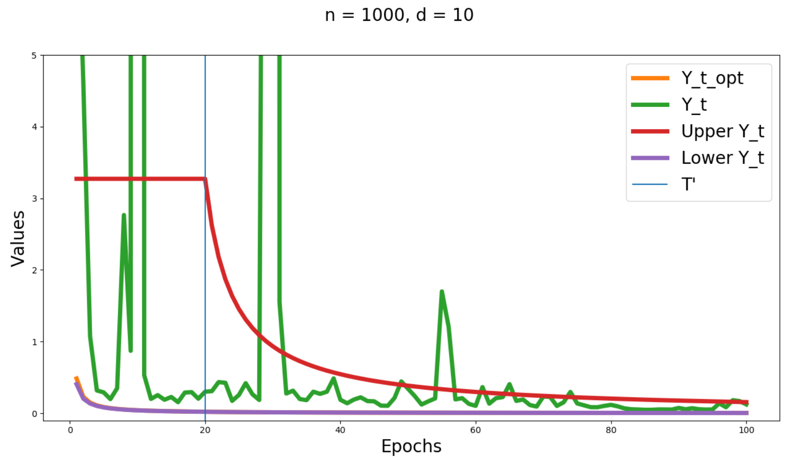
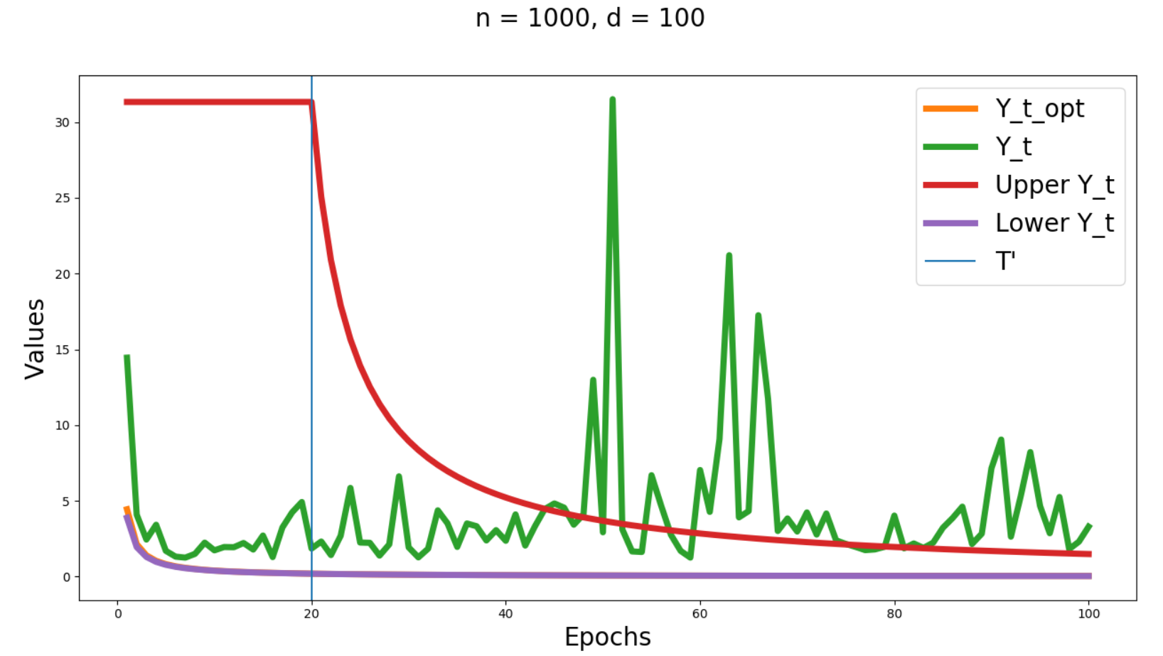
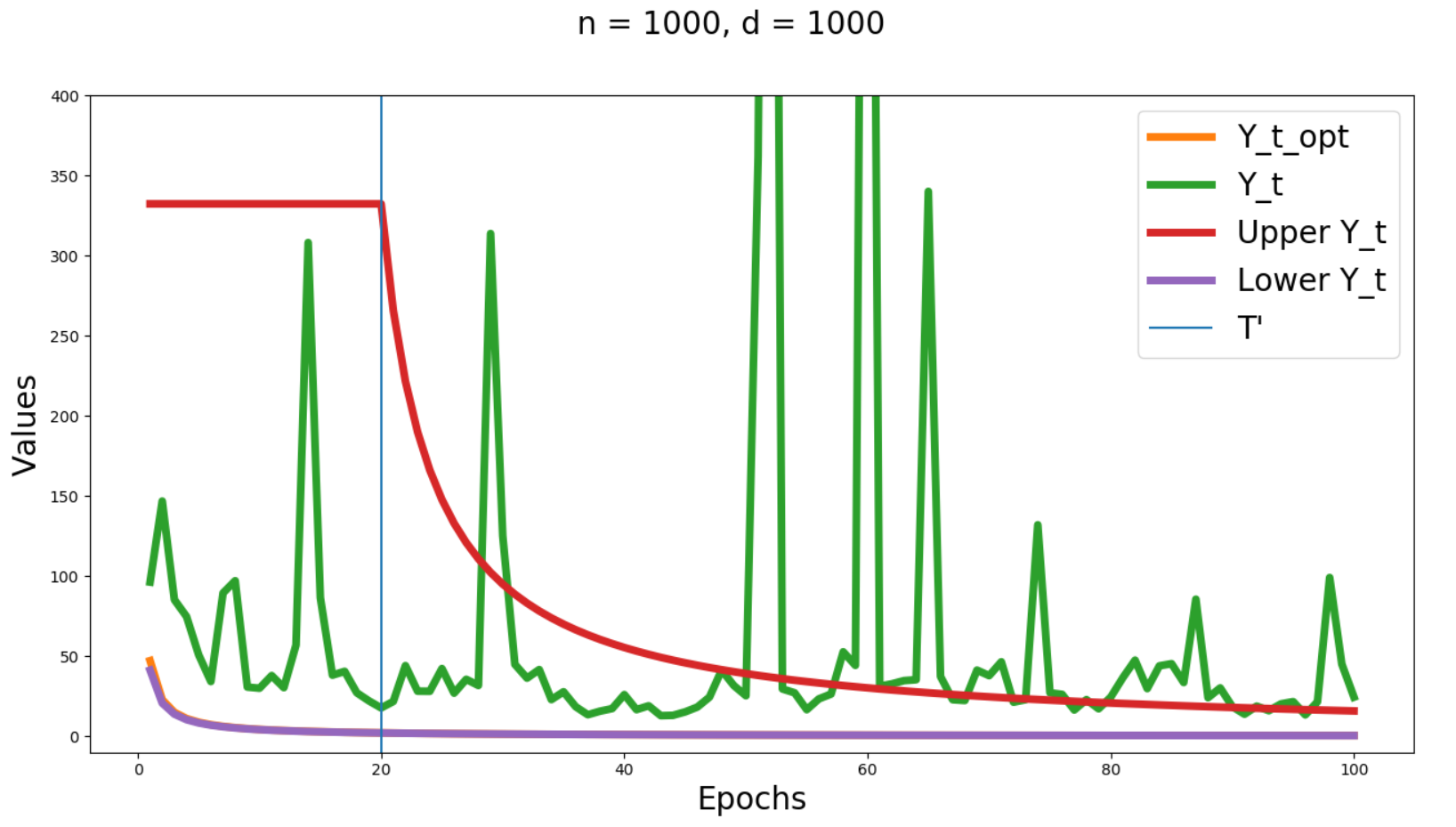
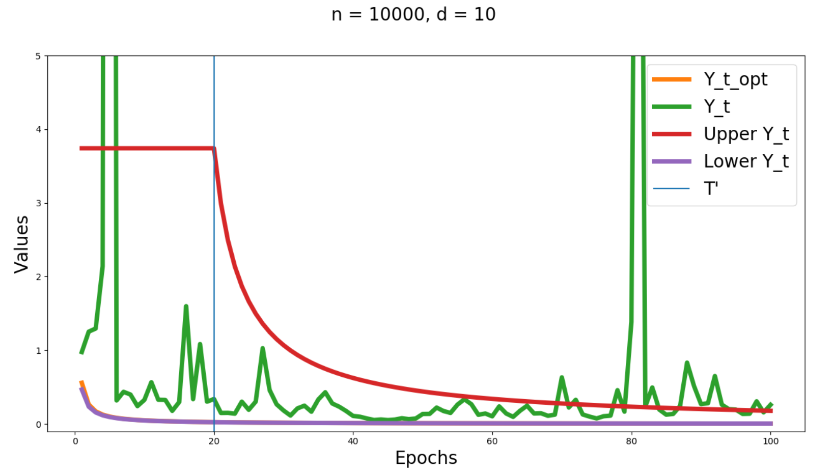
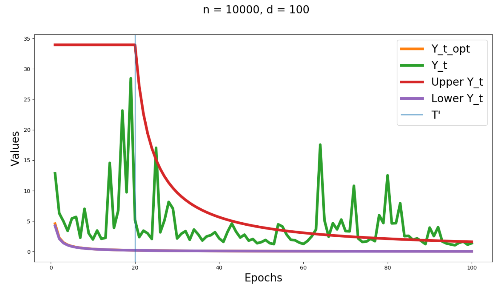
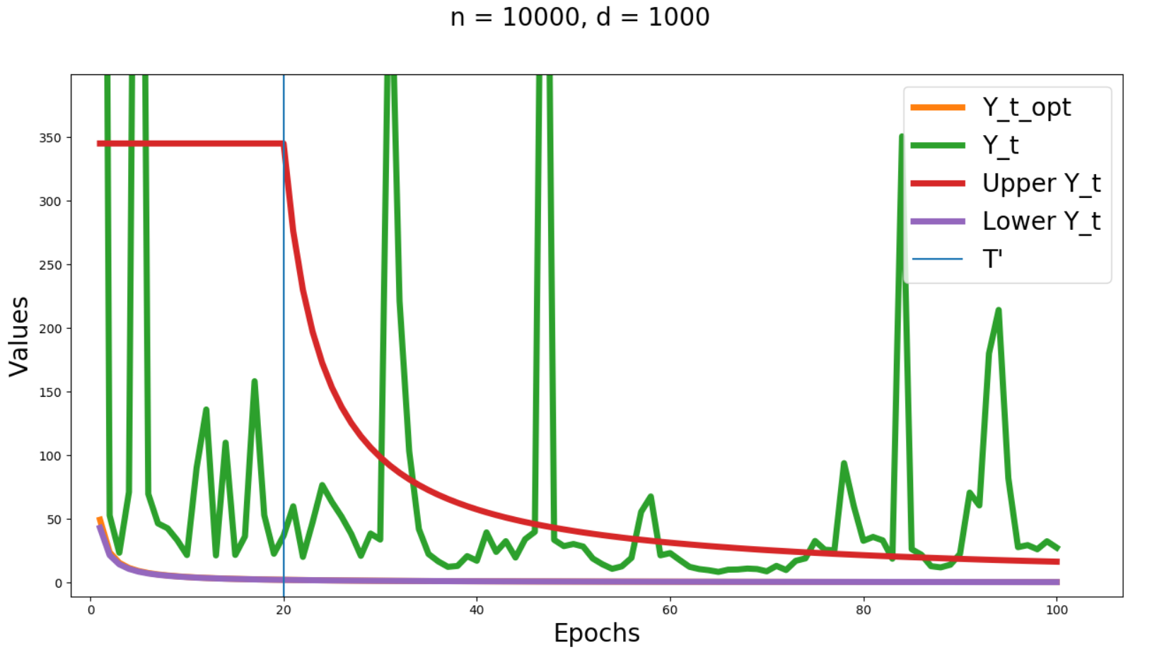
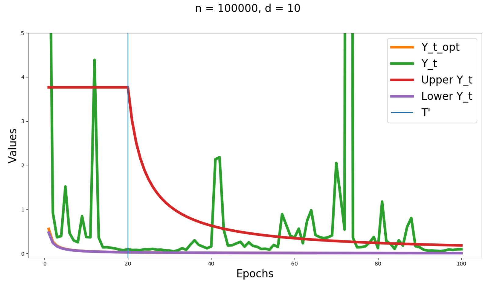
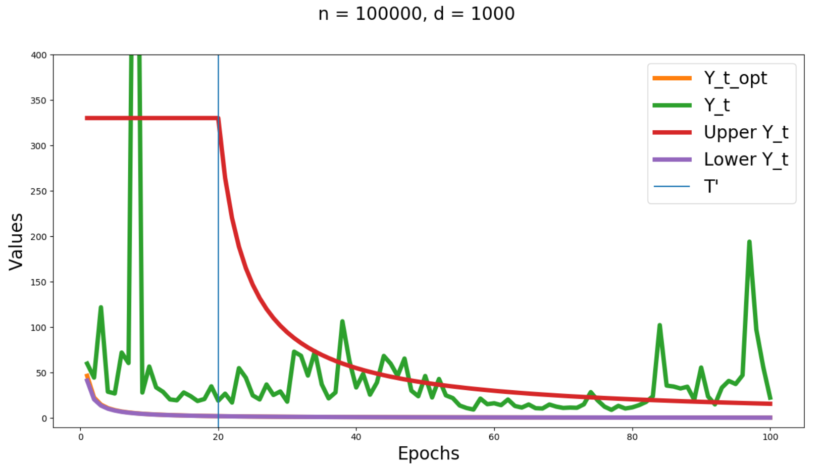
Figure 1: $Y_{t}$ and its upper and lower bounds

We denote the labels “Upper Y$\_$t” (red line) and “Lower Y$\_$t” (violet line) in Figure 1 as the upper and lower bounds of $Y_{t}$ in (22) and (21) respectively (with a vertical line at epoch $20$ because we expect to see the upper bound take effect when $t\geq T^{\prime}=20L/\mu$, see supplemental material A); “Y$\_$t$\_$opt” (orange line) as $Y_{t}$ defined in Theorem 1 computed by using information from oracle ${\cal U}$; “Y$\_$t” (green line) as the squared norm of the difference between $w_{t}$ and $w_{*}$, where $w_{t}$ is generated from Algorithm 1 with learning rate (28). Note that $Y_{t}$ in Figure 1 is computed as average of 10 runs of $\|w_{t}-w_{*}\|^{2}$ (not exactly $\mathbb{E}[\|w_{t}-w_{*}\|^{2}]$).

“Upper Y$\_$t” (red line), “Lower Y$\_$t” (violet line) and “Y$\_$t$\_$opt” (orange line) do not oscillate because they can be correctly computed using formulas (22), (21), and (29), respectively, i.e., they have no variation. The green line “Y$\_$t” for stepsize $\eta_{t}=\frac{2}{\mu t+4L}$ in Figure 1 oscillates because our analysis does not consider the variance of $\|w_{t}-w_{*}\|^{2}$. From (4) we infer that a decrease in $\eta_{t}$ leads to a decrease of the variance of $\|w_{t}-w_{*}\|^{2}$. This fact is reflected in all subfigures in Figure 1. We expect that increasing $d$ and $n$ (the number of dimensions in data and the number of data points) will increase the variance. Hence, it requires larger $t$ to make the variance approach $0$ as shown in Figure 1. For sufficiently large $t$, the optimality of $\eta_{t}=\frac{2}{\mu t+4L}$ is clearly shown in Figure 1 when $n=1000$ and $d=10$, i.e., the green line is in between red line (upper bound) and violet line (lower bound). We note that “Lower Y$\_$t” and “Y$\_$t$\_$opt” are very close to each other in Figure 1 and the difference between them is shown in Figure 2.

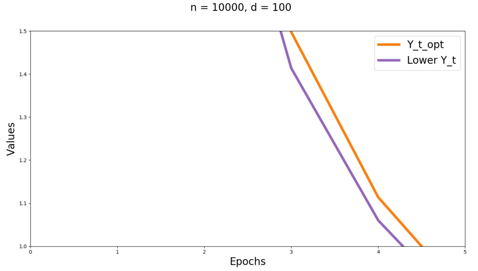
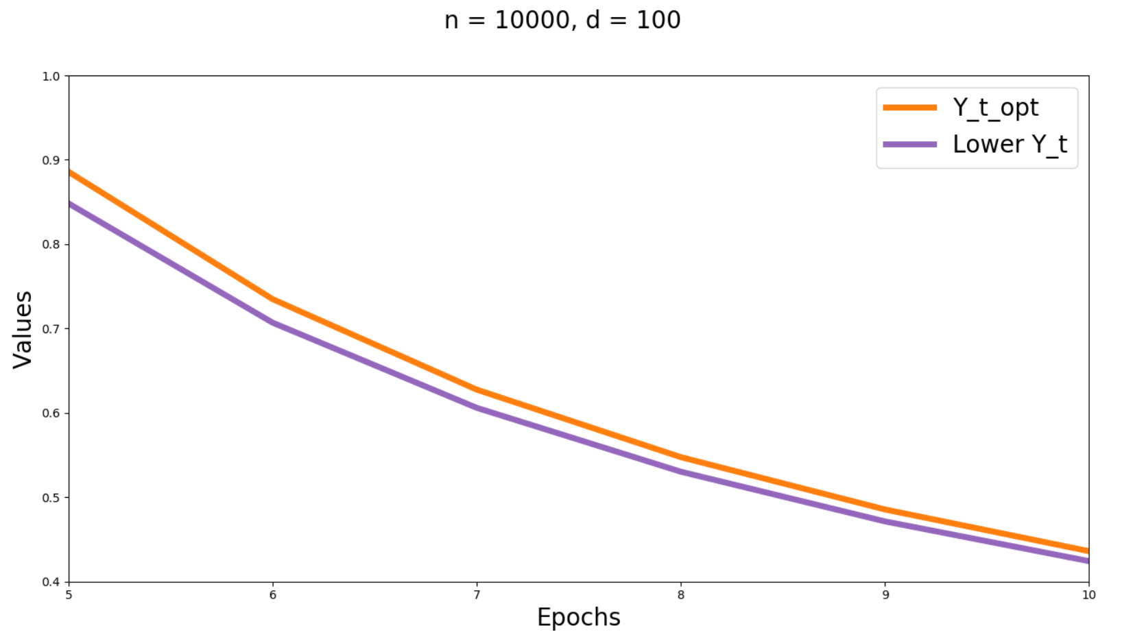
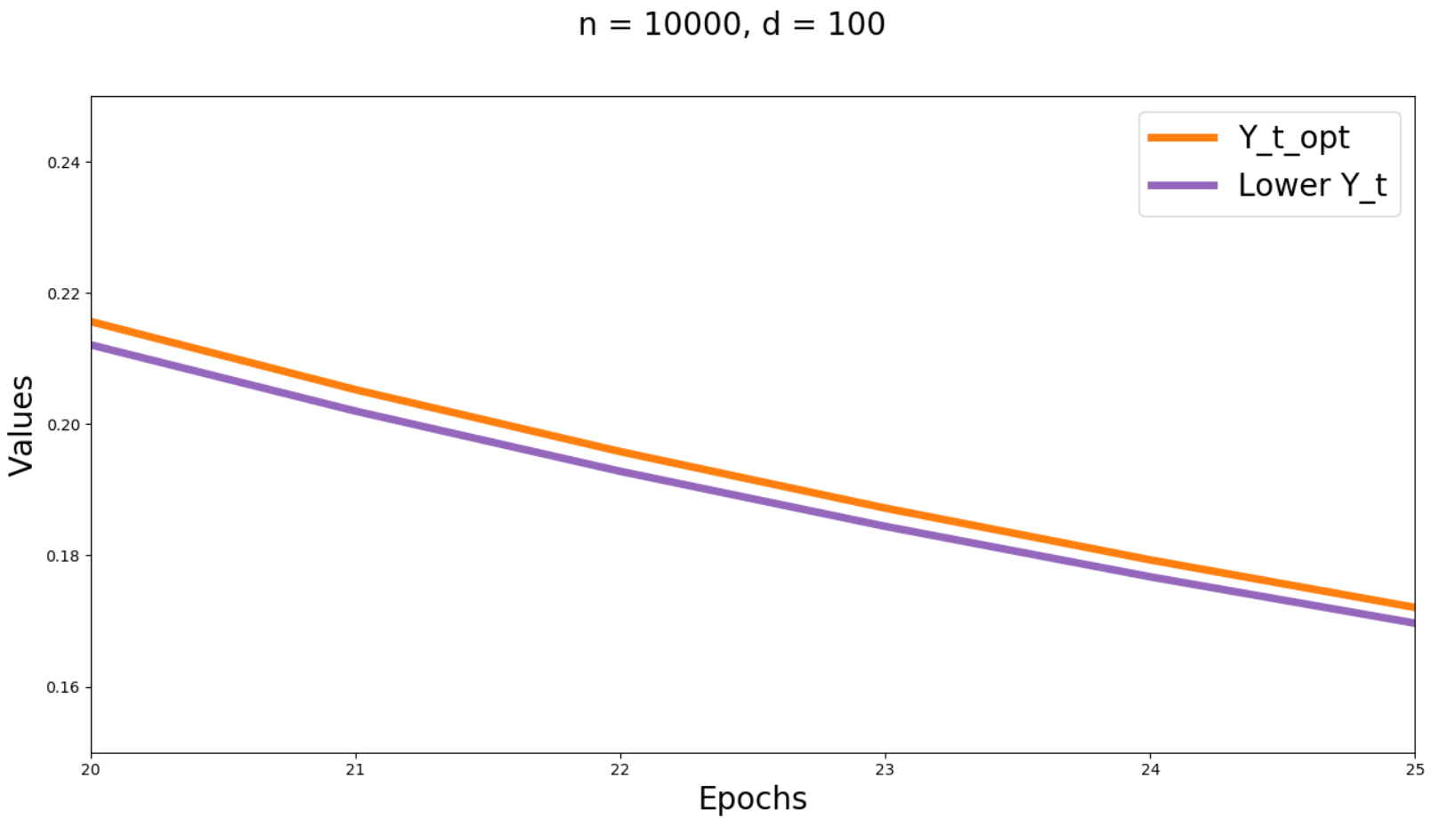
Figure 2: The difference between “Lower Y$\_$t” and “Y$\_$t$\_$opt” ($n=10000$, $d=100$)

Appendix C Related Work

In Agarwal et al. [2009], the authors showed that the lower bound of $Y_{t}$ is $\operatorname{\mathcal{O}}(1/t)$ with bounded gradient assumption for objective function $F$ over a convex set $\mathcal{S}$. To show the lower bound, the authors use the following three assumptions for the objective function $F$:

1. The assumption of a strongly convex objective function, i.e., Assumption 1 (see Definition 3 in Agarwal et al. [2009]).

2. There exists a bounded convex set $\mathcal{S}\subset\mathbb{R}^{d}$ such that

   $$\mathbb{E}[\|\nabla f(w;\xi)\|^{2}]\leq\sigma^{2}$$

   for all $w\in\mathcal{S}\subset\mathbb{R}^{d}$ (see Definition 1 in Agarwal et al. [2009]). Notice that this is not the same as the bounded gradient assumption where $\mathcal{S}=\mathbb{R}^{d}$ is unbounded.

3. The objective function $F$ is a convex Lipschitz function, i.e., there exists a positive number $K$ such that

   $$\|F(w)-F(w^{\prime})\|\leq K\|w-w^{\prime}\|,\forall w,w^{\prime}\in\mathcal{S}\subset\mathbb{R}^{d}.$$

   We notice that this assumption actually implies the assumption on bounded gradients as stated above.

On the existence of the assumption of bounded convex set $\mathcal{S}\subset\mathbb{R}^{d}$ where SGD converges: let us restate the example in Nguyen et al. [2018b], i.e. $F(w)=\frac{1}{2}(f_{1}(w)+f_{2}(w))$ where $f_{1}(w)=\frac{1}{2}w^{2}$ and $f_{2}(w)=w$. It is obvious that $F$ is strongly convex but $f_{1}$ and $f_{2}$ are not. Let $w_{0}=0\in\mathcal{S}$, for any number $t\geq 0$, with probability $\frac{1}{2^{t}}$, the steps of SGD algorithm for all $i<t$ are $w_{i+1}=w_{i}-\eta_{i}$. This implies that $w_{t}=-\sum_{i=1}\eta_{i}$. Since $\sum_{i=1}\eta_{i}=\infty$, $w_{t}$ will escape the set $\mathcal{S}$ when $t$ is sufficiently large. We conclude that in ${\cal F}_{str}$ there are objective functions that can escape any bounded set $\mathcal{S}$ with non-zero probability.

If $\mathcal{S}$ is $\mathbb{R}^{d}$, we have the following results:

On the non-coexistence of the assumption of a bounded gradient over $\mathbb{R}^{d}$ and assumption of having strong convexity: As pointed out in Nguyen et al. [2018b], the assumption of bounded gradient does not co-exist with strongly convex assumption. As shown in Nesterov [2004], Bottou et al. [2016], Assumption 1 on strong convexity implies

$$2\mu[F(w)-F(w_{*})]\leq\|\nabla F(w)\|^{2}\ ,\ \forall w\in\mathbb{R}^{d}.$$ (33)

As shown in Nguyen et al. [2018b], for any $w\in\mathbb{R}^{d}$, we have

$$2\mu[F(w)-F(w_{*})] \overset{(\ref{eq:stronglyconvex})}{\leq}\|\nabla F(w)\|^{2}=\|\mathbb{E}[\nabla f(w;\xi)]\|^{2}$$

$$\leq\mathbb{E}[\|\nabla f(w;\xi)\|^{2}]\leq\sigma^{2}.$$

Therefore,

$$F(w)\leq\frac{\sigma^{2}}{2\mu}+F(w_{*}),\forall w\in\mathbb{R}^{d}.$$

Note that, the from Assumption 1 and $\nabla F(w_{*})=0$, we have

$$F(w)\geq\mu\|w-w_{*}\|^{2}+F(w_{*}),\forall w\in\mathbb{R}^{d}.$$

Clearly, the two last inequalities contradict to each other for sufficiently large $\|w-w_{*}\|^{2}$. Precisely, only when $\sigma$ is equal to $\infty$, then the assumption of bounded gradient and the assumption of strongly convexity of $F$ can co-exist. However, $\sigma$ cannot be $\infty$ and this result implies that there does not exist any objective function $F$ satisfies the assumption of bounded gradients over $\mathbb{R}^{d}$ and the assumption of having a strongly convex objective function at the same time.

On the non-coexistence of the assumption of being convex Lipschitz over $\mathbb{R}^{d}$ and assumption of being strongly convex: Moreover, we can also show that the assumption of convex Lipschitz function does not co-exist with the assumption of being strongly convex. As shown in Section 2.3 in Agarwal et al. [2009], the assumption of Lipschitz function implies that $\|\nabla F(w)\|\leq K,\forall w\in R^{d}$. Hence, by using the same argument from the analysis of the non-coexistence of bounded gradient assumption and assumption of strongly convex, we can conclude that these two assumptions cannot co-exist. In other words, there does not exist an objective function $F$ which satisfies the assumption of convex Lipschitz function and assumption of being strongly convex at the same time.

C.1 Discussion on the usage of Assumptions in Agarwal et al. [2009]

As stated in Section 3 and Section 4.1.1 in Agarwal et al. [2009], the authors construct a class of strongly convex Lipschitz objective function $F$ which has $K=\sigma$. The authors showed that the problem of convex optimization for the constructed class of objective functions $F$ is at least as hard as estimating the biases of $d$ independent coins (i.e., the problem of estimating parameters of Bernoulli variables). As one additional important assumption to prove the lower bound of a first order stochastic algorithm, the authors assume the existence of stepsizes $\eta_{t}$ which make an first order stochastic algorithm converge for a given objective function $F$ under the three aforementioned assumptions (see Lemma 2 in Agarwal et al. [2009]). Note that the proof of the lower bound of $Y_{t}$ is described in Theorem 2 in Agarwal et al. [2009] and Theorem 2 uses their Lemma 2. If their Lemma 2 is not valid, then the proof of the lower bound of $Y_{t}$ in Theorem 2 is also not valid.

Given the proof strategy in Agarwal et al. [2009] of the convergence of a first order stochastic algorithm, one may require that the convex set $\mathcal{S}$ where $F$ has all these nice properties must be $\mathbb{R}^{d}$ as explained above. This, however, will lead to the non-coexistence of bounded gradient assumption and strongly convex assumption and the non-coexistence of Lipschitz function assumption and strongly convex assumption as discussed above. In this case, their Lemma 2 is not valid because of non-existence of an objective function $F$, in which case the proof of lower bound of $Y_{t}$ in Theorem 2 is not correct.

However, we explain why the setup as proposed in Agarwal et al. [2009] may still be acceptable and lead to a proper lower bound: The paper assumes that we only restrict the analysis of SGD in a bounded convex set $\mathcal{S}$ which is not $\mathbb{R}^{d}$, and only in this bounded set $\mathcal{S}$ we assume that objective function acts like a Lipschitz function (implying bounded gradients in ${\cal S}$).

There are two possible cases at the $t$-th iteration a first order stochastic algorithm, the algorithm diverges or converges. Let us define $p_{t}=Pr(w_{t}\notin\mathcal{S})$. Hence, $Pr(w_{t}\in\mathcal{S})=1-p_{t}$. Let

$$Y^{conv}_{t}=\mathbb{E}[\|w_{t}-w_{*}\|^{2}|w_{t}\in\mathcal{S}]$$

and

$$Y^{div}_{t}=\mathbb{E}[\|w_{t}-w_{*}\|^{2}|w_{t}\notin\mathcal{S}].$$

Since $Y_{t}=\mathbb{E}[\|w_{t}-w_{*}\|^{2}$, $Y_{t}$ is equal to

$$Y_{t} =p\cdot Y^{div}_{t}+(1-p)\cdot Y^{conv}_{t}$$

$$\geq p\cdot Y^{conv}_{t}+(1-p)\cdot Y^{conv}_{t}$$

$$\geq Y^{conv}_{t}$$

$$\geq\text{ lower bound in~{}\cite[cite]{\@@bibref{Authors Phrase1YearPhrase2}{AgarwalBartlettRavikumarEtAl}{\@@citephrase{[}}{\@@citephrase{]}}}}.$$

The above derivation hinges on the first inequality where we assume $Y^{div}_{t}\geq Y^{conv}_{t}$. Typically, for strongly convex objective functions and $w_{*},w_{0}\in\mathcal{S}$), it seems always true that $Y^{div}_{t}\geq Y^{conv}_{t}$ because $w_{t}$ gets far from $w_{*}$ for the divergence case and it gets close to $w_{*}$ for the convergence case. Of course a proper proof of this property is still needed in order to rigorously complete the argument leading to the lower bound in Agarwal et al. [2009]. In fact this remains an open problem (one can invent strange corner cases that need extra thought/proof).

The above result is interesting because now we only need to prove the convergence of a first order stochastic algorithm in a certain convex set $\mathcal{S}$ with a certain probability $p$. This is completely different from the proof of convergence of e.g. SGD in the general case as in Moulines and Bach [2011] and Nguyen et al. [2018b], Gower et al. [2019] where we need to prove it with probability 1.

C.2 Setup

We describe the setup of the class of strong convex functions proposed in Agarwal et al. [2009].

As shown in Section 4.1.1 Agarwal et al. [2009], the following two sets are required.

1. Subset $\mathcal{V}\subset\{-1,+1\}^{d}$ and $\mathcal{V}=\{\alpha^{1},\dotsc,\alpha^{M}\}$ with $\Delta_{H}(\alpha^{j},\alpha^{k})\geq\frac{d}{4}$ for all $j\neq k$, where $\Delta_{H}$ denotes the Hamming metric, i.e $\Delta_{H}(\alpha,\beta):=\sum_{i=1}^{d}\mathbb{I}[\alpha_{i}\neq\beta_{i}]$. As discussed by the authors, $|\mathcal{V}|=M\geq(2/\sqrt{e})^{\frac{d}{2}}$.

2. Subset $\mathcal{F}_{base}=\{f^{+}_{i},f^{-}_{i},i=1,\dotsc,d\}$ where $f^{+}_{i},f^{-}_{i}$ will be designed depending on the problem at hand.

Given $\mathcal{V}$, $\mathcal{F}_{base}$ and a constant $\delta\in(0,\frac{1}{4}]$, we define the function class $\mathcal{F}(\delta):=\{F_{\alpha},\alpha\in\mathcal{V}\}$ where

$$F_{\alpha}(w):=\frac{c}{d}\sum_{i=1}^{d}\{(1/2+\alpha_{i}\delta)f^{+}_{i}(w)+(1/2-\alpha_{i}\delta)f^{-}_{i}(w)\}.$$ (34)

The $\mathcal{F}_{base}$ and constant $c$ are chosen in such a way that $\mathcal{F}(\delta)\subset\mathcal{F}$ where $\mathcal{F}$ is the class of strongly convex objective functions defined over set $\mathcal{S}$ and satisfies all the assumptions as mentioned before. In case $\mathcal{F}$ is the class of strongly convex functions, the key idea to compute the lower bound of SGD proposed in Agarwal et al. [2009] by applying Fano’s inequality Yu [1997] and Le Cam’s bound Cover and Thomas [1991], LeCam et al. [1973] is as follows: If an SGD algorithm $\mathcal{M}_{t}$ works well for optimizing a given function $F_{\alpha^{*}},\alpha^{*}\in\mathcal{V}$ with a given oracle $\mathcal{U}$, then there exists a hypothesis test finding $\hat{\alpha}$ such that:

$$\frac{1}{3}\geq\mathrm{Pr}_{\mathcal{U}}[\hat{\alpha}(\mathcal{M}_{t})\neq\alpha]\geq 1-2\frac{16dt\delta^{2}+\log(2)}{d\log(2/\sqrt{e})}.$$ (35)

From (35), we have

$$\frac{16dt\delta^{2}+\log(2)}{d\log(2/\sqrt{e})}\approx\frac{16dt\delta^{2}}{d\log(2/\sqrt{e})}\geq 2/3.$$

Hence,

$$t\geq\frac{\log(2/\sqrt{e})}{48}\frac{1}{\delta^{2}}.$$ (36)

As shown in Section 4.3 Agarwal et al. [2009], to proceed the proof, we set $Y_{t}=\frac{c\delta^{2}r^{2}}{18(1-\theta)}$. Combining with (36) yields

$$Y_{t}\geq\frac{1}{t}\frac{\log(2/\sqrt{e})}{864}\frac{cr^{2}}{1-\theta}.$$ (37)

In addition to the proof of the lower bound, we also need to set $c=\frac{Ld}{rd^{1/p}}$ and $\mu^{2}=\frac{L}{rd^{1/p}}(1-\theta)$ where $\mathcal{S}=\mathrm{B}_{\infty}(r)$. By substituting $c$ and $\mu^{2}$ into (37), we obtain:

$$Y_{t}\geq\frac{1}{t}\frac{\log(2/\sqrt{e})}{864d}\frac{1}{\mu^{2}}c^{2}r^{2}.$$ (38)

To complete the description of the setup in Agarwal et al. [2009], we briefly describe the proposed oracle $\mathcal{U}$ which outputs some information to the SGD algorithm at each iteration for constructing the stepsize $\eta_{t}$. There are two types of oracle $\mathcal{U}$ defined as follows.

1. Oracle $\mathcal{U}_{A}$: 1-dimensional unbiased gradients

   1. Pick an index $i\in{1,\dotsc,d}$ uniformly at random.

   2. Draw $b_{i}\in\{0,1\}$ according to a Bernoulli distribution with parameter $1/2+\alpha_{i}\delta$.

   3. For the given input $x\in\mathcal{S}$, return the value $f_{i}$ and subgradient $\nabla f_{i}$ of the function

      $$f_{i,A}:=c[b_{i}f^{+}_{i}+(1-b_{i})f^{-}_{i}].$$

2. Oracle $\mathcal{U}_{B}$: $d$-dimensional unbiased gradients.

   • For $i=1,\dotsc,d$, draw $b_{i}\in\{0,1\}$ according to a Bernoulli distribution with parameter $1/2+\alpha_{i}\delta$.

   • For the given input $x\in\mathcal{S}$, return the value $f_{i}$ and subgradient $\nabla f_{i}$ of the function

     $$f_{i,B}:=\frac{c}{d}\sum_{i=1}^{d}[b_{i}f^{+}_{i}+(1-b_{i})f^{-}_{i}].$$

C.3 Analysis and Comparison

In this section, we want to compare our lower bound ($\approx\frac{N}{2\mu^{2}t}$) with the one in (38) when $t$ is sufficiently large. In order to do this, we need to compute $N=2\mathbb{E}[\|\nabla f(w^{*};\xi)\|^{2}]$ for the strongly convex function class proposed in Agarwal et al. [2009]. For the strongly convex case, the authors defined the base functions as follows. Given a parameter $\theta\in[0,1)$, we have

$$f^{+}_{i}(w) =r\theta|w_{i}+r|+\frac{1-\theta}{4}(w_{i}+r)^{2},$$

$$f^{-}_{i}(w) =r\theta|w_{i}-r|+\frac{1-\theta}{4}(w_{i}-r)^{2},$$

where $w=(w_{1},\dotsc,w_{d})$. Let $e_{i}$ be $1/2+\alpha_{i}\delta$. Substituting $e_{i}$ in (34) yields $F_{\alpha}(w)=\frac{1}{d}[\sum_{i=1}^{d}f_{\alpha,i}(w)]$ where $f_{\alpha,i}(w)=c[e_{i}f^{+}_{i}(w)+(1-e_{i})f^{-}_{i}(w)]$. Due to the construction of $F_{\alpha}$, the definition of $f_{\alpha,i}(w)$ and the construction of oracle $\mathcal{U}_{A}$ or oracle $\mathcal{U}_{B}$, $w^{*}$ of $F_{\alpha}$ can be found by finding each $w^{*}_{i}$ for each $f_{\alpha,i}(w)$ first. Precisely, we have the following cases:

1. $w_{i}<-r$: we have

   • $f_{\alpha,i}(w)=-r\theta(w_{i}+r)e_{i}+\frac{1-\theta}{4}(w_{i}+r)^{2}e_{i}-r\theta(w_{i}-r)(1-e_{i})+\frac{1-\theta}{4}(w_{i}-r)^{2}(1-e_{i})$.

   • $\nabla f_{\alpha,i}(w)=(1-\theta)e_{i}r-\frac{1+\theta}{2}r+\frac{1-\theta}{2}w_{i}$.

   • $\nabla f_{\alpha,i}(w)=0$ at $w^{-r}_{i}=r[1-2e_{i}+\frac{2\theta}{1-\theta}]$.

2. $-r\leq w_{i}\leq r$: we have

   • $f_{\alpha,i}(w)=r\theta(w_{i}+r)e_{i}+\frac{1-\theta}{4}(w_{i}+r)^{2}e_{i}-r\theta(w_{i}-r)(1-e_{i})+\frac{1-\theta}{4}(w_{i}-r)^{2}(1-e_{i})$.

   • $\nabla f_{\alpha,i}(w)=(1+\theta)e_{i}r-\frac{1+\theta}{2}r+\frac{1-\theta}{2}w_{i}$.

   • $\nabla f_{\alpha,i}(w)=0$ at $w^{[-r,r]}_{i}=r\frac{1+\theta}{1-\theta}(1-2e_{i})$.

3. $r\leq w_{i}\leq\infty$: we have

   • $f_{\alpha,i}(w)=r\theta(w_{i}+r)e_{i}+\frac{1-\theta}{4}(w_{i}+r)^{2}e_{i}+r\theta(w_{i}-r)(1-e_{i})+\frac{1-\theta}{4}(w_{i}-r)^{2}(1-e_{i})$.

   • $\nabla f_{\alpha,i}(w)=(1-\theta)e_{i}r+\frac{3\theta-1}{2}r+\frac{1-\theta}{2}w_{i}$.

   • $\nabla f_{\alpha,i}(w)=0$ at $w^{r}_{i}=r[1-2e_{i}-2\frac{\theta}{1-\theta}]$.

Now, we have five important points $w^{-r}_{i},w^{[-r,r]}_{i},w^{r}_{i},-r$ and $r$ and at these points $F_{\alpha}$ can be minimum. We consider the following cases

1. $\alpha_{i}=-1$ and then $e_{i}=\frac{1}{2}+\alpha_{i}\delta=\frac{1}{2}-\delta$ where $\delta\in[0,1/4)$, we have

   • $w^{-r}_{i}=r[\frac{2\theta}{1-\theta}+2\delta]>-r$.

   • $w^{[-r,r]}_{i}=r\frac{1+\theta}{1-\theta}(2\delta)$. In this case $w^{[-r,r]}_{i}$ may belong $[-r,r]$ or it may be greater than $r$.

   • $w^{r}_{i}=r(2\delta-\frac{2\theta}{1-\theta})<r$ .

   This result implies $F_{\alpha}$ is minimum at $w^{*}_{i}=r$ and $\nabla f_{\alpha,i}(w^{*})=cr[(1-\theta)e_{i}+\theta]=cr[(1-\theta)(1/2-\delta)+\theta]$. Or it can be minimum at $w^{[-r,r]}_{i}$ if $w^{[-r,r]}_{i}\in[-r,r]$ and $\nabla f_{\alpha,i}(w^{*})=0$.

2. $\alpha_{i}=+1$ and then $e_{i}=\frac{1}{2}+\alpha_{i}\delta=\frac{1}{2}+\delta$ where $\delta\in[0,1/4)$, we have

   • $w^{-r}_{i}=r[\frac{2\theta}{1-\theta}-2\delta]$. Since $\frac{2\theta}{1-\theta}-2\delta>-1$ when $\delta\in[0,1/4)$ and $\theta\in[0,1)$. Hence $w^{-r}_{i}>-r$.

   • $w^{[-r,r]}_{i}=r\frac{1+\theta}{1-\theta}(-2\delta)<0$. In this case $w^{[-r,r]}_{i}$ may belong $[-r,r]$ or it may be smaller than $-r$.

   • $w^{r}_{i}=r(-2\delta-\frac{2\theta}{1-\theta})<r$.

   This result implies $F_{\alpha}$ is minimum at $w^{*}_{i}=-r$ and $\nabla f_{\alpha,i}(w^{*})=cr[(1-\theta)e_{i}-1]=cr[(1-\theta)(1/2+\delta)-1]$. Or it can be minimum at $w^{[-r,r]}_{i}$ if $w^{[-r,r]}_{i}\in[-r,r]$ and $\nabla f_{\alpha,i}(w^{*})=0$.

By definition, we have

$$N =2\mathbb{E}[\|\nabla f_{i}(w^{*})\|^{2}]=2\frac{1}{d}\sum_{i=1}^{d}[e_{i}\|c\nabla f^{+}_{i}(w^{*})\|^{2}+(1-e_{i})\|c\nabla f^{-}_{i}(w^{*})\|^{2}]$$

From the analysis above, we have four possible $w^{*}_{i}$, i.e., $-r,r,r\frac{1+\theta}{1-\theta}(-2\delta)$ and $r\frac{1+\theta}{1-\theta}(2\delta)$. If we plug $w^{*}$ which has $w^{*}_{i}=-r$ or $w^{*}_{i}=r$, then we have $[e_{i}\|c\nabla f^{+}_{i}(w^{*})\|^{2}+(1-e_{i})\|c\nabla f^{-}_{i}(w^{*})\|^{2}]=(1/2-\delta)c^{2}r^{2}$. For $w^{*}_{i}$ which has $w^{*}_{i}=r\frac{1+\theta}{1-\theta}(-2\delta)$ or $r\frac{1+\theta}{1-\theta}(2\delta)$, we have $[e_{i}\|c\nabla f^{+}_{i}(w^{*})\|^{2}+(1-e_{i})\|c\nabla f^{-}_{i}(w^{*})\|^{2}]=(1/4-\delta^{2})(1+\theta)^{2}c^{2}r^{2}$. This proves that

$$N=2\beta c^{2}r^{2}$$

with $\beta$ somewhere in the range

$$[(\frac{1}{2}-\delta),(\frac{1}{4}-\delta^{2})(1+\theta)^{2}]\mbox{ or }[(\frac{1}{4}-\delta^{2})(1+\theta)^{2},(\frac{1}{2}-\delta)],$$

where $\delta\in[0,1/4)$ and $\theta\in[0,1)$.

Substituting $N=2\beta c^{2}r^{2}$ into (38) yields

$$Y_{t}\geq\frac{\log(2/\sqrt{e})}{(864\cdot d)(2\beta)}\frac{N}{\mu^{2}t},$$ (39)

which is further minimized by taking

$$\beta=\max\{(\frac{1}{2}-\delta),(\frac{1}{4}-\delta^{2})(1+\theta)^{2}\}.$$

Notice that, given our freedom in choosing $\delta$ and $\theta$, we can minimize $\beta$ as a function of $\delta$ and $\theta$ in order to maximize the lower bound in (39). This gives (in the limit) $\delta=1/4$ with $\theta\leq 2/\sqrt{3}-1=0.155$ leading to $\beta=1/4$. This leads to the final lower bound

$$Y_{t}\geq\frac{\log(2/\sqrt{e})}{432\cdot d}\frac{N}{\mu^{2}t}.$$

Clearly, the lower bound in is much smaller than our lower bound of $\approx\frac{N}{2\mu^{2}t}$ when $t$ is sufficiently large. Moreover, this lower bound depends on $1/d$ and it becomes smaller when $d$ increases.

References

- Agarwal et al. (2009) Alekh Agarwal, Martin J Wainwright, Peter L Bartlett, and Pradeep K Ravikumar. Information-theoretic lower bounds on the oracle complexity of convex optimization. In Advances in Neural Information Processing Systems, pages 1–9, 2009.
- Bertsekas (1999) D.P. Bertsekas. Nonlinear Programming. Athena Scientific, 1999.
- Bottou et al. (2016) Léon Bottou, Frank E Curtis, and Jorge Nocedal. Optimization methods for large-scale machine learning. arXiv:1606.04838, 2016.
- Boyd and Vandenberghe (2004) Stephen Boyd and Lieven Vandenberghe. Convex Optimization. Cambridge University Press, 2004.
- Cover and Thomas (1991) Thomas M. Cover and Joy A. Thomas. Elements of Information Theory. Wiley-Interscience, New York, NY, USA, 1991. ISBN 0-471-06259-6.
- Defazio et al. (2014) Aaron Defazio, Francis Bach, and Simon Lacoste-Julien. SAGA: A fast incremental gradient method with support for non-strongly convex composite objectives. In NIPS, pages 1646–1654, 2014.
- Duchi et al. (2011) John Duchi, Elad Hazan, and Yoram Singer. Adaptive subgradient methods for online learning and stochastic optimization. Journal of Machine Learning Research, 12(Jul):2121–2159, 2011.
- Gower et al. (2019) Robert Mansel Gower, Nicolas Loizou, Xun Qian, Alibek Sailanbayev, Egor Shulgin, and Peter Richtarik. Sgd: General analysis and improved rates. arXiv preprint arXiv:1901.09401, 2019.
- Hastie et al. (2009) Trevor Hastie, Robert Tibshirani, and Jerome Friedman. The Elements of Statistical Learning: Data Mining, Inference, and Prediction. Springer Series in Statistics, 2nd edition, 2009.
- Johnson and Zhang (2013) Rie Johnson and Tong Zhang. Accelerating stochastic gradient descent using predictive variance reduction. In NIPS, pages 315–323, 2013.
- Kingma and Ba (2014) Diederik P Kingma and Jimmy Ba. Adam: A method for stochastic optimization. arXiv preprint arXiv:1412.6980, 2014.
- Le Roux et al. (2012) Nicolas Le Roux, Mark Schmidt, and Francis Bach. A stochastic gradient method with an exponential convergence rate for finite training sets. In NIPS, pages 2663–2671, 2012.
- Leblond et al. (2018) Rémi Leblond, Fabian Pederegosa, and Simon Lacoste-Julien. Improved asynchronous parallel optimization analysis for stochastic incremental methods. arXiv preprint arXiv:1801.03749, 2018.
- LeCam et al. (1973) Lucien LeCam et al. Convergence of estimates under dimensionality restrictions. The Annals of Statistics, 1(1):38–53, 1973.
- Moulines and Bach (2011) Eric Moulines and Francis R Bach. Non-asymptotic analysis of stochastic approximation algorithms for machine learning. In Advances in Neural Information Processing Systems, pages 451–459, 2011.
- Nemirovsky A.S. and IUdin (c1983.) Arkadii Semenovich. Nemirovsky A.S. and D. B. IUdin. Problem complexity and method efficiency in optimization /. Wiley,, Chichester ;, c1983. "A Wiley-Interscience publication.".
- Nesterov (2004) Yurii Nesterov. Introductory lectures on convex optimization : a basic course. Applied optimization. Kluwer Academic Publ., Boston, Dordrecht, London, 2004. ISBN 1-4020-7553-7.
- Nguyen et al. (2018a) Lam Nguyen, Phuong Ha Nguyen, Peter Richtarik, Katya Scheinberg, Martin Takac, and Marten van Dijk. New convergence aspects of stochastic gradient algorithms. arXiv preprint arXiv:1811.12403, 2018a.
- Nguyen et al. (2018b) Lam Nguyen, Phuong Ha Nguyen, Marten van Dijk, Peter Richtarik, Katya Scheinberg, and Martin Takac. SGD and hogwild! Convergence without the bounded gradients assumption. In ICML, 2018b.
- Nguyen et al. (2017) Lam M. Nguyen, Jie Liu, Katya Scheinberg, and Martin Takáč. SARAH: A novel method for machine learning problems using stochastic recursive gradient. In ICML, 2017.
- Nocedal and Wright (2006) Jorge Nocedal and Stephen J. Wright. Numerical Optimization. Springer, New York, 2nd edition, 2006.
- Raginsky and Rakhlin (2011) Maxim Raginsky and Alexander Rakhlin. Information-Based Complexity, Feedback and Dynamics in Convex Programming. IEEE Trans. Information Theory, 57(10):7036–7056, 2011.
- Robbins and Monro (1951) Herbert Robbins and Sutton Monro. A stochastic approximation method. The Annals of Mathematical Statistics, 22(3):400–407, 1951.
- Schmidt and Roux (2013) Mark Schmidt and Nicolas Le Roux. Fast convergence of stochastic gradient descent under a strong growth condition. arXiv preprint arXiv:1308.6370, 2013.
- Sutskever et al. (2013) Ilya Sutskever, James Martens, George Dahl, and Geoffrey Hinton. On the importance of initialization and momentum in deep learning. In International conference on machine learning, pages 1139–1147, 2013.
- Yu (1997) Bin Yu. Assouad, Fano, and Le Cam. In Festschrift for Lucien Le Cam, pages 423–435. Springer, 1997.
- Zou et al. (2018) Fangyu Zou, Li Shen, Zequn Jie, Weizhong Zhang, and Wei Liu. A Sufficient Condition for Convergences of Adam and RMSProp. arXiv preprint arXiv:1811.09358, 2018.