Velocity Dependence from Resonant Self-Interacting Dark Matter
Abstract
The dark matter density distribution in small-scale astrophysical objects may indicate that dark matter is self-interacting, while observations from clusters of galaxies suggest that the corresponding cross section depends on the velocity. Using a model-independent approach, we show that resonant self-interacting dark matter (RSIDM) can naturally explain such a behavior. In contrast to what is often assumed, this does not require a light mediator. We present explicit realizations of this mechanism and discuss the corresponding astrophysical constraints.
Dark matter (DM) makes up more than 80% of the matter in the Universe today and played a crucial role in forming stars and galaxies, and hence us. Yet its nature is unknown. Currently the best pieces of information come from astrophysical observations. N-body simulations of collisionless DM predict astrophysical halos with DM density following a universal profile that scales as in its outskirts but exhibits a central cusp, , with , referred to as the Navarro-Frenk-White (NFW) profile Dubinski:1991bm ; Navarro:1995iw ; Navarro:1996gj . Nevertheless, many studies show hints of a DM mass deficit in the inner regions of certain halos. Notably, observations indicate that numerous dwarf galaxies Moore:1994yx ; Flores:1994gz ; Walker:2011zu and some low-surface-brightness spiral galaxies deBlok:2001hbg ; deBlok:2002vgq ; Simon:2004sr have a shallower central DM density, better described by a core of constant density, i.e., by . This is known as the core-vs-cusp problem. Although it is more pressing in small-scale objects, shallower DM density profiles –with a slope of – have been reported for certain galaxy clusters Sand:2003bp ; Newman:2012nw . Moreover, the DM mass deficit also manifests itself in halos that are less dense than what simulations suggest if they host the galaxies that we observe. This is the too-big-to-fail problem, observed for the subhalos of the Milky Way BoylanKolchin:2011de , Andromeda Tollerud:2014zha and the Local Group Kirby:2014sya .
Several explanations for these discrepancies have been discussed in the literature. The systematic uncertainties introduced in deriving DM distributions from observations of luminous objects are one of them. Most importantly, the motions of HI gas and stars may not be faithful tracers of the DM circular velocity Blok:2002tr ; Rhee:2003vw ; Gentile:2005de ; Spekkens:2005ik ; Valenzuela:2005dh ; Dalcanton:2010bp ; Kormendy:2014ova ; 2016MNRAS.462.3628R ; Maccio:2016egb ; 2017A&A…601A…1P ; Brooks:2017rfe ; Oman:2017vkl ; 2018MNRAS.474.1398G ; Read:2018pft . Baryonic processes are another conceivable explanation for the discrepancies, since the aforementioned simulations only include collisionless DM. Solutions along this line include supernova-driven baryonic winds Navarro:1996bv ; Gelato:1998hb ; Binney:2000zt ; Gnedin:2001ec , DM heating due to star formation Read:2018fxs , infalling baryonic clumps ElZant:2001re ; Weinberg:2001gm ; Ahn:2004xt ; Tonini:2006gwz as well as active galactic nuclei or black holes Martizzi:2011aa . Nonetheless, there is no consensus on why systematic uncertainties or baryonic processes lead to a seemingly universal mass deficit at various scales.
A more exciting possibility consists of considering DM collisions in the inner regions of astrophysical objects Spergel:1999mh . This is known as self-interacting dark matter (SIDM). N-body simulations Dave:2000ar ; Vogelsberger:2012ku ; Rocha:2012jg ; Peter:2012jh ; Elbert:2014bma ; Fry:2015rta confirm that DM scattering processes indeed reduce the central density of DM halos, providing a solution to both problems 111Besides, SIDM can also explain the diversity of galaxy rotation curves Oman:2015xda ; Kamada:2016euw ; Creasey:2016jaq ; Robertson:2017mgj .. For a recent review see Tulin:2017ara .
The observed mass deficit is more appreciable in small-scale halos, where the DM velocity dispersion is relatively low. Therefore, a self-scattering cross section that decreases with the DM velocity can better fit observations Kaplinghat:2015aga , although a constant cross section is certainly not excluded due to the large uncertainties mentioned above. A long-range force induced by a light boson interacting with DM is often invoked to obtain a velocity-dependent cross section Spergel:1999mh ; Feng:2009hw . Other possibilities that do not involve a light mediator include exothermic inelastic scatterings McDermott:2017vyk ; Vogelsberger:2018bok and self-heating DM Kamada:2017gfc ; Chu:2018nki ; Kamada:2018hte .
The essence of this work is to discuss the resonant self-interaction of DM (RSIDM) as another mechanism for achieving the desired velocity dependence of SIDM. Such a resonant behavior was firstly discussed for DM annihilation in Griest:1990kh ; Gondolo:1990dk ; Jungman:1995df ; Feldman:2008xs ; Pospelov:2008jd ; Ibe:2008ye ; MarchRussell:2008tu ; Guo:2009aj ; Ibe:2009dx ; Kakizaki:2005en ; Arina:2014fna , and applied to DM self-scattering in specific scenarios Ibe:2009mk ; Braaten:2013tza ; Duch:2017nbe ; Braaten:2018xuw . Nevertheless, the velocity dependence of resonant self-scattering and its general astrophysical consequences have not been explored in detail. In this letter, we do so in a model-independent way, and show that resonant scattering is able to address the observed DM mass deficit at all astrophysical scales. Concrete DM scenarios and indirect searches are discussed later.
Resonant scattering in DM halos. Numerous studies claim that the density distribution of certain DM halos do not follow a NFW profile in the inner region. In the SIDM hypothesis, this is due to DM collisions that thermalize the DM particles in such a region thereby reducing its average density Spergel:1999mh . Hence the inner profile is closely related to the velocity-averaged scattering cross section per unit of DM mass, , where 222 For resonant scattering, nearly equals the momentum-transfer cross section, , and we do not differentiate between them here.
| (1) |
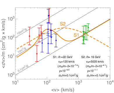
Here, is the relative velocity, which we assume to follow a Maxwell-Boltzmann distribution truncated at the escape velocity, , of the corresponding halo. is a parameter related to the average relative velocity via . Notice that in dwarf galaxies km/s whereas in clusters of galaxies km/s.
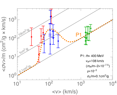
A semi-analytical method has been proposed in Kaplinghat:2015aga to infer the value of for a given DM halo from observational data. The method was applied to five clusters from Newman:2012nw , seven low-surface-brightness spiral galaxies in KuziodeNaray:2007qi and six dwarf galaxies of the THINGS sample Oh:2010ea (also see Elbert:2016dbb ; Valli:2017ktb ). Fig. 1 shows their results in green, blue and red, respectively. The values presented here are for illustrative purpose, and should be taken with caution due to the large uncertainties in extracting the cross sections from kinematical data. See e.g. sokolenko:2018noz for a recent study. Nonetheless, at face value, the figure demonstrates that a cross section independent of the velocity –the ones corresponding to the diagonal lines– can hardly accommodate all points. Notice that the values of at cluster scales are in agreement with observations from the Bullet Cluster giving Randall:2007ph ; Robertson:2016xjh , which is one of the strongest constraints on DM self-interactions.
Barring the uncertainties, the figure suggests that the cross section depends on . In this letter, we propose that this is due to RSIDM. This takes place when there exists an intermediate particle, denoted as , so that the total self-scattering cross section can be cast as a sum of a constant piece, , plus a Breit-Wigner resonance 333Note that the interference term only exists for -wave scattering. For the cases discussed here, that term was found to be negligible with respect to the second term of Eq. (2). Furthermore, it changes its sign from below to above resonance and hence nearly cancels out upon integration over the velocity profile.. More explicitly, for non-relativistic DM,
| (2) |
where the total kinetic energy and symmetry factor read
| and | (3) |
Here, and are the spins of the resonance and the DM particles, respectively. is the reduced mass. If DM has internal degrees of freedom other than its spin, they must be accounted for in . The collision hits the resonance when and hence .
In addition, the width in Eq. (2) can be calculated in terms of the resonance self-energy by means of . This, as well as the denominator in Eq. (2), assumes that the total width is dominated by the process . Besides that, Eq. (2) is completely general as it directly follows from unitarity considerations of the scattering matrix Breit:1936zzb . In perturbative theories, the running width can be written as 444 This can be proven using effective range theory Bethe:1949yr .
| (4) |
Here, is the orbital angular momentum, is the decay rate, and a constant characterizes the coupling between the resonance and DM. The factor accounts for the phase space and possible angular momentum suppression. Then we find , where a dimensionless
| (5) |
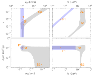
determines the non-trivial velocity-dependence of the resonant self-scattering. For -wave and -wave scatterings, we calculate the best-fit parameter sets S1, S2, and P1 based on the inferred data from Ref. Kaplinghat:2015aga and show them in Fig. 1 555 Using a similar method, has been estimated for eight Milky Way dwarfs Valli:2017ktb . A proper combined fit including those results is beyond the scope of this letter. Nevertheless, since such dwarf galaxies have all approximately the same , a combined fit would not change our conclusions regarding the velocity dependence of . . is fitted with the other parameters for S1 and P1 while for S2 a negligible is taken as a prior. They all lead to , in contrast to for the fit assuming only a constant cross section (we treat errors as uncorrelated). For S1 and P1, we show the 95% C.L. contours in Fig. 2. Many comments are in order.
First, we have numerically checked that a precise knowledge of the escape velocity is not necessary for calculating . This is because Eq. (5) converges quite fast due to the Boltzmann factor. In fact, as shown in the supplementary material, exact solutions exist in the limit , which will be implicitly applied hereafter for simplicity.
Second, to qualitatively understand Figs. 1 and 2, one can use the narrow-width approximation (NWA)
| (6) |
It works very well for because . In this case, we find that scales as at , and as at . In both regions, can not be much larger than one. Therefore, the resonant effect is negligible except for the intermediate region, where the NWA captures the velocity dependence as
| (7) |
Notice that the peak lies at as illustrated by P1 in Fig. 1. The corresponding line actually applies to any , because the dependence on can be absorbed by rescaling . Using Eq. (7) we find that the best-fit parameters at 95% C.L. for are given by
| (8) | |||
| (9) |
Such values for the velocity correspond to . The regions where all this applies are shown in Fig. 2. For -wave scattering, demanding leads to . Moreover, a perturbative around cmg requires sub-GeV DM masses unless . Interestingly, P1 predicts at . In fact, scatterings with can realize small cross sections at very low velocities. Hence, the recent claim based on Draco observations Read:2018pft is consistent with RSIDM.
As long as , the NWA also applies for -wave scattering. For , is proportional to (to ) below (above) , because such large values of broaden the resonance. S1 and S2 illustrate the narrow and the broad width cases, respectively.
In conclusion, resonant scattering is able to address the observed DM mass deficit at all astrophysical scales.
| Scenario | Interaction Lagrangian | |||||
|---|---|---|---|---|---|---|
| I | 0 | 0- | ||||
| IIa | 0 | 0 | 0+ | |||
| IIb | 1 | 0 | 1- | |||
| III | 2 | 0 | 2+ | 5 |
RSIDM Models. Below we illustrate the previous model-independent results in concrete RSIDM scenarios. We first introduce a Lagrangian specifying the coupling of the DM to the resonance (see Table 1) and calculate the cross section and the self-energy. We subsequently corroborate that they can be cast as Eqs. (2) and (4) show. The scenarios are:
I. Fermionic DM with a pseudoscalar mediator. The scattering process is -wave while . The corresponding best fit is thus S2. Notice that a light pseudoscalar mediator does not lead to SIDM because it induces a suppressed Yukawa potential (see e.g. Kahlhoefer:2017umn ). Due to this and because it leads to velocity-suppressed direct-detection rates, this candidate is phenomenologically interesting.
II. Dark mesons. In QCD-like theories, DM can be a dark pion. Analogous to real pions, it can be a triplet , with . If is a dark resonance (IIa), the scattering takes place via the -wave, where we expect GeV DM and . The best fit is thus S2. If is a dark resonance (IIb), the scattering is -wave suppressed. The constant piece of the cross section is given by in perturbation theory, but it is plausible that there are other contributions. We therefore leave as a free parameter. The corresponding best-fit curve is P1. We expect in this case. In the same fashion, minimal QCD-like theories can also lead to spin-1 DM Francis:2018xjd . In all cases, DM can be produced by means of the SIMP Dolgov:1980uu ; Carlson:1992fn ; Hochberg:2014dra ; Yamanaka:2014pva ; Hochberg:2014kqa ; Bernal:2015bla ; Bernal:2015lbl ; Lee:2015gsa ; Choi:2015bya ; Hansen:2015yaa ; Bernal:2015xba ; Kuflik:2015isi ; Hochberg:2015vrg ; Choi:2016hid ; Pappadopulo:2016pkp ; Farina:2016llk ; Choi:2016tkj ; Dey:2016qgf ; Cline:2017tka ; Choi:2017mkk ; Choi:2017zww ; Chu:2017msm ; Choi:2018iit and the freeze-in McDonald:2001vt ; Hall:2009bx ; Bernal:2015ova mechanisms.
III. Tensor resonances. They also arise in strongly-coupled theories. Despite the potential complications of such theories, the generality of our approach allows to describe the scattering induced by a spin-2 resonance 666Not to be confused with the Ricci tensor.. If this couples to the DM energy-momentum tensor with a cut-off scale , and taking scalar DM as an example, we find that the corresponding Feynman rules Han:1998sg indeed lead to a -wave cross section given by Eq. (2). For , we obtain keV DM with . The corresponding best fit is given by P1 in Fig. 1 after rescaling the mass by means of Eq. (9).
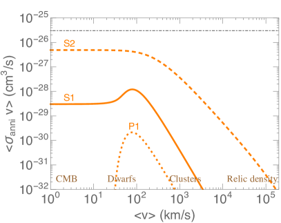
Annihilation vs. Scattering. It is not necessary that the DM annihilates, as e.g. in models of asymmetric DM. Nonetheless, if the resonance decays into a pair of Standard Model (SM) particles , in analogy to Eq. (2), the resonant DM annihilation into has a cross section
| (10) |
where is the decay width for . As above, we assume that the resonance dominantly decays to a pair of DM particles, and thus that the contribution of to the imaginary part of the resonance self-energy, , is subleading. This is different from Ibe:2009mk , in which the resonance dominantly decays into visible particles. As expected for annihilations (but not for elastic scatterings), as long as . Furthermore, for the cases where NWA applies, . In contrast, for broad -wave resonances such as S2, where , gets enhanced by another factor .
The coupling to light charged particles is mostly constrained by Fermi-LAT observations of local satellites Ackermann:2013yva ; Fermi-LAT:2016uux and the Planck data on the cosmic microwave background (CMB) Ade:2015xua ; Liu:2016cnk . For instance, the corresponding Fermi-LAT upper limit on for GeV DM is of the order of . For S2, this leads to an upper limit on the branching ratio, , of about –. This bound is much stronger than that of S1 and P1, due to the enhancement factor mentioned above. Motivated by this, we conservatively fix and calculate the annihilation cross section as a function of for the same parameter sets of Fig. 1. The result is shown in Fig. 3. Therefore, the resonance can only couple feebly to light charged particles, which is why the SIDM candidates with thermal freeze-out from Duch:2017nbe are excluded. Of course this is model-dependent. For instance, if the resonance only couples to neutrinos, the bound on becomes much weaker, and larger are thus allowed.
Furthermore, the strong velocity dependence of suggests that the usual freeze-out can hardly work, as for SIDM with light mediators decaying into visible particles Bringmann:2016din ; Binder:2017lkj ; Hufnagel:2017dgo ; Hufnagel:2018bjp . Nevertheless, the DM abundance might arise from other SIDM production mechanisms Bernal:2015ova . Indeed, for the -wave case, producing the DM abundance with small couplings is possible via freeze-in McDonald:2001vt ; Hall:2009bx or 4-to-2 annihilations Bernal:2015xba , where a scalar (vector) resonance can feebly mix with the Higgs (SM gauge bosons). See Essig:2013lka ; Bernal:2017kxu for reviews.
Discussion. We advocate the resonant scattering as a possible SIDM realization with a velocity-dependent scattering cross section. Instead of a light mediator, this RSIDM scenario requires a near-threshold resonance with ranging from for narrow resonances to for -wave scattering with broad widths. Such resonances exist in Nature. As an example, particles resonantly scatter by means of Be in exactly the same way as described above. In fact, these processes were the main subject of the original article by Breit and Wigner Breit:1936zzb and they may as well occur in the DM sector. Actually, dark nucleons as SIDM have been studied in Braaten:2018xuw 777Their findings suggest that their model is described by S2.. Furthermore, lattice studies suggest that QCD-like theories of DM might possess such states Briceno:2017max .
Conclusions. We find that this RSIDM hypothesis can certainly address the core-vs-cusp and the too-to-big-fail problems while still being in agreement with cluster observations. We have also discussed indirect detection signatures, which are nevertheless model-dependent. Additionally, we would like to emphasize that usual SIMPs –which are often said to be disfavored because their scattering cross section does not vary with velocity– can easily accommodate the mechanism proposed here.
Acknowledgements.
Acknowledgements. We thank Ranjan Laha and Kai Schmidt-Hoberg for interesting discussions. X.C. is supported by the ‘New Frontiers’ program of the Austrian Academy of Sciences. C.G.C. is supported by the ERC Starting Grant NewAve (638528). H.M. thanks the Alexander von Humboldt Foundation for support while this work was completed. H.M. was supported by the NSF grant PHY-1638509, by the U.S. DOE Contract DE-AC02-05CH11231, by the JSPS Grant-in-Aid for Scientific Research (C) (17K05409), MEXT Grant-in-Aid for Scientific Research on Innovative Areas (15H05887, 15K21733), by WPI, MEXT, Japan, and by the Binational Science Foundation (grant No. 2016153).References
- (1) J. Dubinski and R. G. Carlberg, “The Structure of cold dark matter halos,” Astrophys. J. 378 (1991) 496.
- (2) J. F. Navarro, C. S. Frenk, and S. D. M. White, “The Structure of cold dark matter halos,” Astrophys. J. 462 (1996) 563–575, arXiv:astro-ph/9508025.
- (3) J. F. Navarro, C. S. Frenk, and S. D. M. White, “A Universal density profile from hierarchical clustering,” Astrophys. J. 490 (1997) 493–508, arXiv:astro-ph/9611107.
- (4) B. Moore, “Evidence against dissipationless dark matter from observations of galaxy haloes,” Nature 370 (1994) 629.
- (5) R. A. Flores and J. R. Primack, “Observational and theoretical constraints on singular dark matter halos,” Astrophys. J. 427 (1994) L1–4, arXiv:astro-ph/9402004.
- (6) M. G. Walker and J. Penarrubia, “A Method for Measuring (Slopes of) the Mass Profiles of Dwarf Spheroidal Galaxies,” Astrophys. J. 742 (2011) 20, arXiv:1108.2404.
- (7) W. J. G. de Blok, S. S. McGaugh, A. Bosma, and V. C. Rubin, “Mass density profiles of LSB galaxies,” Astrophys. J. 552 (2001) L23–L26, arXiv:astro-ph/0103102.
- (8) W. J. G. de Blok and A. Bosma, “High-resolution rotation curves of low surface brightness galaxies,” Astron. Astrophys. 385 (2002) 816, arXiv:astro-ph/0201276.
- (9) J. D. Simon, A. D. Bolatto, A. Leroy, L. Blitz, and E. L. Gates, “High-resolution measurements of the halos of four dark matter-dominated galaxies: Deviations from a universal density profile,” Astrophys. J. 621 (2005) 757–776, arXiv:astro-ph/0412035.
- (10) D. J. Sand, T. Treu, G. P. Smith, and R. S. Ellis, “The dark matter distribution in the central regions of galaxy clusters: Implications for CDM,” Astrophys. J. 604 (2004) 88–107, arXiv:astro-ph/0309465.
- (11) A. B. Newman, T. Treu, R. S. Ellis, and D. J. Sand, “The Density Profiles of Massive, Relaxed Galaxy Clusters: II. Separating Luminous and Dark Matter in Cluster Cores,” Astrophys. J. 765 (2013) 25, arXiv:1209.1392.
- (12) M. Boylan-Kolchin, J. S. Bullock, and M. Kaplinghat, “Too big to fail? The puzzling darkness of massive Milky Way subhaloes,” Mon. Not. Roy. Astron. Soc. 415 (2011) L40, arXiv:1103.0007.
- (13) E. J. Tollerud, M. Boylan-Kolchin, and J. S. Bullock, “M31 Satellite Masses Compared to LCDM Subhaloes,” Mon. Not. Roy. Astron. Soc. 440 (2014) no. 4, 3511–3519, arXiv:1403.6469.
- (14) E. N. Kirby, J. S. Bullock, M. Boylan-Kolchin, M. Kaplinghat, and J. G. Cohen, “The dynamics of isolated Local Group galaxies,” Mon. Not. Roy. Astron. Soc. 439 (2014) no. 1, 1015–1027, arXiv:1401.1208.
- (15) M. Kaplinghat, S. Tulin, and H.-B. Yu, “Dark Matter Halos as Particle Colliders: Unified Solution to Small-Scale Structure Puzzles from Dwarfs to Clusters,” Phys. Rev. Lett. 116 (2016) no. 4, 041302, arXiv:1508.03339.
- (16) W. J. G. d. Blok, A. Bosma, and S. S. McGaugh, “Simulating observations of dark matter dominated galaxies: towards the optimal halo profile,” Mon. Not. Roy. Astron. Soc. 340 (2003) 657–678, arXiv:astro-ph/0212102.
- (17) G. Rhee, A. Klypin, and O. Valenzuela, “The Rotation curves of dwarf galaxies: A Problem for cold dark matter?,” Astrophys. J. 617 (2004) 1059–1076, arXiv:astro-ph/0311020.
- (18) G. Gentile, A. Burkert, P. Salucci, U. Klein, and F. Walter, “The dwarf galaxy DDO 47 as a dark matter laboratory: testing cusps hiding in triaxial halos,” Astrophys. J. Lett. 634 (2005) L145–L148, arXiv:astro-ph/0506538.
- (19) K. Spekkens and R. Giovanelli, “The Cusp/core problem in Galactic halos: Long-slit spectra for a large dwarf galaxy sample,” Astron. J. 129 (2005) 2119–2137, arXiv:astro-ph/0502166.
- (20) O. Valenzuela, G. Rhee, A. Klypin, F. Governato, G. Stinson, T. R. Quinn, and J. Wadsley, “Is there evidence for flat cores in the halos of dwarf galaxies?: the case of ngc 3109 and ngc 6822,” Astrophys. J. 657 (2007) 773–789, arXiv:astro-ph/0509644.
- (21) J. J. Dalcanton and A. Stilp, “Pressure Support in Galaxy Disks: Impact on Rotation Curves and Dark Matter Density Profiles,” Astrophys. J. 721 (2010) 547–561, arXiv:1007.2535.
- (22) J. Kormendy and K. C. Freeman, “Scaling Laws for Dark Matter Halos in Late-type and Dwarf Spheroidal Galaxies,” Astrophys. J. 817 (2016) no. 2, 84, arXiv:1411.2170.
- (23) J. I. Read, G. Iorio, O. Agertz, and F. Fraternali, “Understanding the shape and diversity of dwarf galaxy rotation curves in CDM,”Mon. Not. Roy. Astron. Soc. 462 (Nov., 2016) 3628–3645, arXiv:1601.05821.
- (24) A. V. Macciò, S. M. Udrescu, A. A. Dutton, A. Obreja, L. Wang, G. R. Stinson, and X. Kang, “NIHAO X: reconciling the local galaxy velocity function with cold dark matter via mock HI observations,” Mon. Not. Roy. Astron. Soc. 463 (2016) no. 1, L69–L73, arXiv:1607.01028.
- (25) E. Papastergis and A. A. Ponomareva, “Testing core creation in hydrodynamical simulations using the HI kinematics of field dwarfs,”Astronomy & Astrophysics 601 (May, 2017) A1, arXiv:1608.05214.
- (26) A. M. Brooks, E. Papastergis, C. R. Christensen, F. Governato, A. Stilp, T. R. Quinn, and J. Wadsley, “How to Reconcile the Observed Velocity Function of Galaxies with Theory,” Astrophys. J. 850 (2017) no. 1, 97, arXiv:1701.07835.
- (27) K. A. Oman, A. Marasco, J. F. Navarro, C. S. Frenk, J. Schaye, and A. Benítez-Llambay, “Apparent cores and non-circular motions in the HI discs of simulated galaxies,” arXiv:1706.07478.
- (28) A. Genina, A. Benítez-Llambay, C. S. Frenk, S. Cole, A. Fattahi, J. F. Navarro, K. A. Oman, T. Sawala, and T. Theuns, “The core-cusp problem: a matter of perspective,””Mon. Not. Roy. Astron. Soc.” 474 (Feb., 2018) 1398–1411.
- (29) J. I. Read, M. G. Walker, and P. Steger, “The case for a cold dark matter cusp in Draco,” arXiv:1805.06934.
- (30) J. F. Navarro, V. R. Eke, and C. S. Frenk, “The cores of dwarf galaxy halos,” Mon. Not. Roy. Astron. Soc. 283 (1996) L72–L78, arXiv:astro-ph/9610187.
- (31) S. Gelato and J. Sommer-Larsen, “On ddo154 and cold dark matter halo profiles,” Mon. Not. Roy. Astron. Soc. 303 (1999) 321–328, arXiv:astro-ph/9806289.
- (32) J. Binney, O. Gerhard, and J. Silk, “The Dark matter problem in disk galaxies,” Mon. Not. Roy. Astron. Soc. 321 (2001) 471, arXiv:astro-ph/0003199.
- (33) O. Y. Gnedin and H. Zhao, “Maximum feedback and dark matter profiles of dwarf galaxies,” Mon. Not. Roy. Astron. Soc. 333 (2002) 299, arXiv:astro-ph/0108108.
- (34) J. I. Read, M. G. Walker, and P. Steger, “Dark matter heats up in dwarf galaxies,” arXiv:1808.06634.
- (35) A. El-Zant, I. Shlosman, and Y. Hoffman, “Dark halos: the flattening of the density cusp by dynamical friction,” Astrophys. J. 560 (2001) 636, arXiv:astro-ph/0103386.
- (36) M. D. Weinberg and N. Katz, “Bar-driven dark halo evolution: a resolution of the cusp-core controversy,” Astrophys. J. 580 (2002) 627–633, arXiv:astro-ph/0110632.
- (37) K.-J. Ahn and P. R. Shapiro, “Formation and evolution of the self-interacting dark matter halos,” Mon. Not. Roy. Astron. Soc. 363 (2005) 1092–1124, arXiv:astro-ph/0412169.
- (38) C. Tonini and A. Lapi, “Angular momentum transfer in dark matter halos: erasing the cusp,” Astrophys. J. 649 (2006) 591–598, arXiv:astro-ph/0603051.
- (39) D. Martizzi, R. Teyssier, B. Moore, and T. Wentz, “The effects of baryon physics, black holes and AGN feedback on the mass distribution in clusters of galaxies,” Mon. Not. Roy. Astron. Soc. 422 (2012) 3081, arXiv:1112.2752.
- (40) D. N. Spergel and P. J. Steinhardt, “Observational evidence for selfinteracting cold dark matter,” Phys. Rev. Lett. 84 (2000) 3760–3763, arXiv:astro-ph/9909386.
- (41) R. Dave, D. N. Spergel, P. J. Steinhardt, and B. D. Wandelt, “Halo properties in cosmological simulations of selfinteracting cold dark matter,” Astrophys. J. 547 (2001) 574–589, arXiv:astro-ph/0006218.
- (42) M. Vogelsberger, J. Zavala, and A. Loeb, “Subhaloes in Self-Interacting Galactic Dark Matter Haloes,” Mon. Not. Roy. Astron. Soc. 423 (2012) 3740, arXiv:1201.5892.
- (43) M. Rocha, A. H. G. Peter, J. S. Bullock, M. Kaplinghat, S. Garrison-Kimmel, J. Onorbe, and L. A. Moustakas, “Cosmological Simulations with Self-Interacting Dark Matter I: Constant Density Cores and Substructure,” Mon. Not. Roy. Astron. Soc. 430 (2013) 81–104, arXiv:1208.3025.
- (44) A. H. G. Peter, M. Rocha, J. S. Bullock, and M. Kaplinghat, “Cosmological Simulations with Self-Interacting Dark Matter II: Halo Shapes vs. Observations,” Mon. Not. Roy. Astron. Soc. 430 (2013) 105, arXiv:1208.3026.
- (45) O. D. Elbert, J. S. Bullock, S. Garrison-Kimmel, M. Rocha, J. Oñorbe, and A. H. G. Peter, “Core formation in dwarf haloes with self-interacting dark matter: no fine-tuning necessary,” Mon. Not. Roy. Astron. Soc. 453 (2015) no. 1, 29–37, arXiv:1412.1477.
- (46) A. B. Fry, F. Governato, A. Pontzen, T. Quinn, M. Tremmel, L. Anderson, H. Menon, A. M. Brooks, and J. Wadsley, “All about baryons: revisiting SIDM predictions at small halo masses,” Mon. Not. Roy. Astron. Soc. 452 (2015) no. 2, 1468–1479, arXiv:1501.00497.
- (47) S. Tulin and H.-B. Yu, “Dark Matter Self-interactions and Small Scale Structure,” Phys. Rept. 730 (2018) 1–57, arXiv:1705.02358.
- (48) J. L. Feng, M. Kaplinghat, and H.-B. Yu, “Halo Shape and Relic Density Exclusions of Sommerfeld-Enhanced Dark Matter Explanations of Cosmic Ray Excesses,” Phys. Rev. Lett. 104 (2010) 151301, arXiv:0911.0422.
- (49) S. D. McDermott, “Is Self-Interacting Dark Matter Undergoing Dark Fusion?,” Phys. Rev. Lett. 120 (2018) no. 22, 221806, arXiv:1711.00857.
- (50) M. Vogelsberger, J. Zavala, K. Schutz, and T. R. Slatyer, “Evaporating the Milky Way halo and its satellites with inelastic self-interacting dark matter,” arXiv:1805.03203.
- (51) A. Kamada, H. J. Kim, H. Kim, and T. Sekiguchi, “Self-Heating Dark Matter via Semiannihilation,” Phys. Rev. Lett. 120 (2018) no. 13, 131802, arXiv:1707.09238.
- (52) X. Chu and C. Garcia-Cely, “Core formation from self-heating dark matter,” JCAP 1807 (2018) no. 07, 013, arXiv:1803.09762.
- (53) A. Kamada, H. J. Kim, and H. Kim, “Self-heating of Strongly Interacting Massive Particles,” Phys. Rev. D98 (2018) no. 2, 023509, arXiv:1805.05648.
- (54) K. Griest and D. Seckel, “Three exceptions in the calculation of relic abundances,” Phys. Rev. D43 (1991) 3191–3203.
- (55) P. Gondolo and G. Gelmini, “Cosmic abundances of stable particles: Improved analysis,” Nucl. Phys. B360 (1991) 145–179.
- (56) G. Jungman, M. Kamionkowski, and K. Griest, “Supersymmetric dark matter,” Phys. Rept. 267 (1996) 195–373, arXiv:hep-ph/9506380.
- (57) D. Feldman, Z. Liu, and P. Nath, “PAMELA Positron Excess as a Signal from the Hidden Sector,” Phys. Rev. D79 (2009) 063509, arXiv:0810.5762.
- (58) M. Pospelov and A. Ritz, “Astrophysical Signatures of Secluded Dark Matter,” Phys. Lett. B671 (2009) 391–397, arXiv:0810.1502.
- (59) M. Ibe, H. Murayama, and T. T. Yanagida, “Breit-Wigner Enhancement of Dark Matter Annihilation,” Phys. Rev. D79 (2009) 095009, arXiv:0812.0072.
- (60) J. D. March-Russell and S. M. West, “WIMPonium and Boost Factors for Indirect Dark Matter Detection,” Phys. Lett. B676 (2009) 133–139, arXiv:0812.0559.
- (61) W.-L. Guo and Y.-L. Wu, “Enhancement of Dark Matter Annihilation via Breit-Wigner Resonance,” Phys. Rev. D79 (2009) 055012, arXiv:0901.1450.
- (62) M. Ibe, Y. Nakayama, H. Murayama, and T. T. Yanagida, “Nambu-Goldstone Dark Matter and Cosmic Ray Electron and Positron Excess,” JHEP 04 (2009) 087, arXiv:0902.2914.
- (63) M. Kakizaki, S. Matsumoto, Y. Sato, and M. Senami, “Significant effects of second KK particles on LKP dark matter physics,” Phys. Rev. D71 (2005) 123522, arXiv:hep-ph/0502059.
- (64) C. Arina, T. Bringmann, J. Silk, and M. Vollmann, “Enhanced Line Signals from Annihilating Kaluza-Klein Dark Matter,” Phys. Rev. D90 (2014) no. 8, 083506, arXiv:1409.0007.
- (65) M. Ibe and H.-b. Yu, “Distinguishing Dark Matter Annihilation Enhancement Scenarios via Halo Shapes,” Phys. Lett. B692 (2010) 70–73, arXiv:0912.5425.
- (66) E. Braaten and H. W. Hammer, “Universal Two-body Physics in Dark Matter near an S-wave Resonance,” Phys. Rev. D88 (2013) 063511, arXiv:1303.4682.
- (67) M. Duch and B. Grzadkowski, “Resonance enhancement of dark matter interactions: the case for early kinetic decoupling and velocity dependent resonance width,” JHEP 09 (2017) 159, arXiv:1705.10777.
- (68) E. Braaten, D. Kang, and R. Laha, “Production of dark-matter bound states in the early universe by three-body recombination,” arXiv:1806.00609.
- (69) R. Kuzio de Naray, S. S. McGaugh, and W. J. G. de Blok, “Mass Models for Low Surface Brightness Galaxies with High Resolution Optical Velocity Fields,” Astrophys. J. 676 (2008) 920–943, arXiv:0712.0860.
- (70) S.-H. Oh, W. J. G. de Blok, E. Brinks, F. Walter, and R. C. Kennicutt, Jr, “Dark and luminous matter in THINGS dwarf galaxies,” Astron. J. 141 (2011) 193, arXiv:1011.0899.
- (71) O. D. Elbert, J. S. Bullock, M. Kaplinghat, S. Garrison-Kimmel, A. S. Graus, and M. Rocha, “A Testable Conspiracy: Simulating Baryonic Effects on Self-Interacting Dark Matter Halos,” Astrophys. J. 853 (2018) no. 2, 109, arXiv:1609.08626.
- (72) M. Valli and H.-B. Yu, “Dark matter self-interactions from the internal dynamics of dwarf spheroidals,” arXiv:1711.03502.
- (73) A. Sokolenko, K. Bondarenko, T. Brinckmann, J. Zavala, M. Vogelsberger, T. Bringmann, and A. Boyarsky, “Towards an improved model of self-interacting dark matter haloes,” arXiv:1806.11539.
- (74) S. W. Randall, M. Markevitch, D. Clowe, A. H. Gonzalez, and M. Bradac, “Constraints on the Self-Interaction Cross-Section of Dark Matter from Numerical Simulations of the Merging Galaxy Cluster 1E 0657-56,” Astrophys. J. 679 (2008) 1173–1180, arXiv:0704.0261.
- (75) A. Robertson, R. Massey, and V. Eke, “What does the Bullet Cluster tell us about self-interacting dark matter?,” Mon. Not. Roy. Astron. Soc. 465 (2017) no. 1, 569–587, arXiv:1605.04307.
- (76) G. Breit and E. Wigner, “Capture of Slow Neutrons,” Phys. Rev. 49 (1936) 519–531.
- (77) F. Kahlhoefer, K. Schmidt-Hoberg, and S. Wild, “Dark matter self-interactions from a general spin-0 mediator,” JCAP 1708 (2017) no. 08, 003, arXiv:1704.02149.
- (78) A. Francis, R. J. Hudspith, R. Lewis, and S. Tulin, “Dark Matter from Strong Dynamics: The Minimal Theory of Dark Baryons,” arXiv:1809.09117.
- (79) A. D. Dolgov, “ON CONCENTRATION OF RELICT THETA PARTICLES. (IN RUSSIAN),” Yad. Fiz. 31 (1980) 1522–1528.
- (80) E. D. Carlson, M. E. Machacek, and L. J. Hall, “Self-interacting dark matter,” Astrophys. J. 398 (1992) 43–52.
- (81) Y. Hochberg, E. Kuflik, T. Volansky, and J. G. Wacker, “Mechanism for Thermal Relic Dark Matter of Strongly Interacting Massive Particles,” Phys. Rev. Lett. 113 (2014) 171301, arXiv:1402.5143.
- (82) N. Yamanaka, S. Fujibayashi, S. Gongyo, and H. Iida, “Dark matter in the hidden gauge theory,” arXiv:1411.2172.
- (83) Y. Hochberg, E. Kuflik, H. Murayama, T. Volansky, and J. G. Wacker, “Model for Thermal Relic Dark Matter of Strongly Interacting Massive Particles,” Phys. Rev. Lett. 115 (2015) no. 2, 021301, arXiv:1411.3727.
- (84) N. Bernal, C. Garcia-Cely, and R. Rosenfeld, “WIMP and SIMP Dark Matter from the Spontaneous Breaking of a Global Group,” JCAP 1504 (2015) no. 04, 012, arXiv:1501.01973.
- (85) N. Bernal, C. Garcia-Cely, and R. Rosenfeld, “ WIMP and SIMP Dark Matter from a Global U(1) Breaking,” Nucl. Part. Phys. Proc. 267-269 (2015) 353–355.
- (86) H. M. Lee and M.-S. Seo, “Communication with SIMP dark mesons via Z’ -portal,” Phys. Lett. B748 (2015) 316–322, arXiv:1504.00745.
- (87) S.-M. Choi and H. M. Lee, “SIMP dark matter with gauged symmetry,” JHEP 09 (2015) 063, arXiv:1505.00960.
- (88) M. Hansen, K. Langæble, and F. Sannino, “SIMP model at NNLO in chiral perturbation theory,” Phys. Rev. D92 (2015) no. 7, 075036, arXiv:1507.01590.
- (89) N. Bernal and X. Chu, “ SIMP Dark Matter,” JCAP 1601 (2016) 006, arXiv:1510.08527.
- (90) E. Kuflik, M. Perelstein, N. R.-L. Lorier, and Y.-D. Tsai, “Elastically Decoupling Dark Matter,” Phys. Rev. Lett. 116 (2016) no. 22, 221302, arXiv:1512.04545.
- (91) Y. Hochberg, E. Kuflik, and H. Murayama, “SIMP Spectroscopy,” JHEP 05 (2016) 090, arXiv:1512.07917.
- (92) S.-M. Choi and H. M. Lee, “Resonant SIMP dark matter,” Phys. Lett. B758 (2016) 47–53, arXiv:1601.03566.
- (93) D. Pappadopulo, J. T. Ruderman, and G. Trevisan, “Dark matter freeze-out in a nonrelativistic sector,” Phys. Rev. D94 (2016) no. 3, 035005, arXiv:1602.04219.
- (94) M. Farina, D. Pappadopulo, J. T. Ruderman, and G. Trevisan, “Phases of Cannibal Dark Matter,” JHEP 12 (2016) 039, arXiv:1607.03108.
- (95) S.-M. Choi, Y.-J. Kang, and H. M. Lee, “On thermal production of self-interacting dark matter,” JHEP 12 (2016) 099, arXiv:1610.04748.
- (96) U. K. Dey, T. N. Maity, and T. S. Ray, “Light Dark Matter through Assisted Annihilation,” arXiv:1612.09074.
- (97) J. Cline, H. Liu, T. Slatyer, and W. Xue, “Enabling Forbidden Dark Matter,” arXiv:1702.07716.
- (98) S.-M. Choi, H. M. Lee, and M.-S. Seo, “Cosmic abundances of SIMP dark matter,” JHEP 04 (2017) 154, arXiv:1702.07860.
- (99) S.-M. Choi, Y. Hochberg, E. Kuflik, H. M. Lee, Y. Mambrini, H. Murayama, and M. Pierre, “Vector SIMP dark matter,” arXiv:1707.01434.
- (100) X. Chu and C. Garcia-Cely, “Self-interacting Spin-2 Dark Matter,” Phys. Rev. D96 (2017) no. 10, 103519, arXiv:1708.06764.
- (101) S.-M. Choi, H. M. Lee, P. Ko, and A. Natale, “Resolving phenomenological problems with strongly-interacting-massive-particle models with dark vector resonances,” Phys. Rev. D98 (2018) no. 1, 015034, arXiv:1801.07726.
- (102) J. McDonald, “Thermally generated gauge singlet scalars as selfinteracting dark matter,” Phys. Rev. Lett. 88 (2002) 091304, arXiv:hep-ph/0106249.
- (103) L. J. Hall, K. Jedamzik, J. March-Russell, and S. M. West, “Freeze-In Production of FIMP Dark Matter,” JHEP 03 (2010) 080, arXiv:0911.1120.
- (104) N. Bernal, X. Chu, C. Garcia-Cely, T. Hambye, and B. Zaldivar, “Production Regimes for Self-Interacting Dark Matter,” JCAP 1603 (2016) no. 03, 018, arXiv:1510.08063.
- (105) T. Han, J. D. Lykken, and R.-J. Zhang, “On Kaluza-Klein states from large extra dimensions,” Phys. Rev. D59 (1999) 105006, arXiv:hep-ph/9811350.
- (106) Fermi-LAT, M. Ackermann et al., “Dark matter constraints from observations of 25 Milky Way satellite galaxies with the Fermi Large Area Telescope,” Phys. Rev. D89 (2014) 042001, arXiv:1310.0828.
- (107) DES, Fermi-LAT, A. Albert et al., “Searching for Dark Matter Annihilation in Recently Discovered Milky Way Satellites with Fermi-LAT,” Astrophys. J. 834 (2017) no. 2, 110, arXiv:1611.03184.
- (108) Planck, P. A. R. Ade et al., “Planck 2015 results. XIII. Cosmological parameters,” Astron. Astrophys. 594 (2016) A13, arXiv:1502.01589.
- (109) H. Liu, T. R. Slatyer, and J. Zavala, “Contributions to cosmic reionization from dark matter annihilation and decay,” Phys. Rev. D94 (2016) no. 6, 063507, arXiv:1604.02457.
- (110) T. Bringmann, F. Kahlhoefer, K. Schmidt-Hoberg, and P. Walia, “Strong constraints on self-interacting dark matter with light mediators,” Phys. Rev. Lett. 118 (2017) no. 14, 141802, arXiv:1612.00845.
- (111) T. Binder, M. Gustafsson, A. Kamada, S. M. R. Sandner, and M. Wiesner, “Reannihilation of self-interacting dark matter,” Phys. Rev. D97 (2018) no. 12, 123004, arXiv:1712.01246.
- (112) M. Hufnagel, K. Schmidt-Hoberg, and S. Wild, “BBN constraints on MeV-scale dark sectors. Part I. Sterile decays,” JCAP 1802 (2018) 044, arXiv:1712.03972.
- (113) M. Hufnagel, K. Schmidt-Hoberg, and S. Wild, “BBN constraints on MeV-scale dark sectors. Part II. Electromagnetic decays,” arXiv:1808.09324.
- (114) R. Essig et al., “Working Group Report: New Light Weakly Coupled Particles,” in Proceedings, 2013 Community Summer Study on the Future of U.S. Particle Physics: Snowmass on the Mississippi (CSS2013): Minneapolis, MN, USA, July 29-August 6, 2013. 2013. arXiv:1311.0029. http://www.slac.stanford.edu/econf/C1307292/docs/IntensityFrontier/NewLight-17.pdf.
- (115) N. Bernal, M. Heikinheimo, T. Tenkanen, K. Tuominen, and V. Vaskonen, “The Dawn of FIMP Dark Matter: A Review of Models and Constraints,” Int. J. Mod. Phys. A32 (2017) no. 27, 1730023, arXiv:1706.07442.
- (116) R. A. Briceno, J. J. Dudek, and R. D. Young, “Scattering processes and resonances from lattice QCD,” Rev. Mod. Phys. 90 (2018) no. 2, 025001, arXiv:1706.06223.
- (117) K. A. Oman et al., “The unexpected diversity of dwarf galaxy rotation curves,” Mon. Not. Roy. Astron. Soc. 452 (2015) no. 4, 3650–3665, arXiv:1504.01437.
- (118) A. Kamada, M. Kaplinghat, A. B. Pace, and H.-B. Yu, “How the Self-Interacting Dark Matter Model Explains the Diverse Galactic Rotation Curves,” Phys. Rev. Lett. 119 (2017) no. 11, 111102, arXiv:1611.02716.
- (119) P. Creasey, O. Sameie, L. V. Sales, H.-B. Yu, M. Vogelsberger, and J. Zavala, “Spreading out and staying sharp creating diverse rotation curves via baryonic and self-interaction effects,” Mon. Not. Roy. Astron. Soc. 468 (2017) no. 2, 2283–2295, arXiv:1612.03903.
- (120) A. Robertson et al., “The diverse density profiles of galaxy clusters with self-interacting dark matter plus baryons,” Mon. Not. Roy. Astron. Soc. 476 (2018) no. 1, L20–L24, arXiv:1711.09096.
- (121) H. A. Bethe, “Theory of the Effective Range in Nuclear Scattering,” Phys. Rev. 76 (1949) 38–50.
Appendix A Supplementary Material
Here we solve Eq. (5) of the main text for . In the narrow width approximation, i.e. when the second term in the denominator is much smaller than the first one, we can do the replacement
| (11) |
This leads to
| (12) |
which is valid for . If , which is the region of interest in this work, this approximation is very good for any . We have corroborated this numerically. For , such an approximation does not always work. That is however not a problem because there is an exact formula in terms of the exponential integral function, Ei, defined by the principal value of .
For this, let us first notice that when one can rearrange the denominator of Eq. (5) of the main text in terms of the integrals
| (13) |
which are defined for and real. Specifically
| (14) | ||||
where the plus sign applies for and the negative one for . (For simplicity, we do not report the expression for the narrow range ). Finally, can be calculated by means of
| (15) | ||||
Moreover, by analytically extending the previous expression, we can calculate the other integral. This is
| (16) | ||||
As a check, one can take the limit and recover the narrow width approximation of Eq. (12).