A direct approach to imaging in a waveguide with perturbed geometry

Abstract

We introduce a direct, linear sampling approach to imaging in an acoustic waveguide with sound hard walls. The waveguide terminates at one end and has unknown geometry due to compactly supported wall deformations. The goal of imaging is to determine these deformations and to identify localized scatterers in the waveguide, using a remote array of sensors that emits time harmonic probing waves and records the echoes. We present a theoretical analysis of the imaging approach and illustrate its performance with numerical simulations.

1 Introduction and formulation of the problem

Sensor array imaging in waveguides has applications in underwater acoustics [34, 3], nondestructive evaluation of slender structures [16, 27], imaging of and in tunnels [29, 21, 4], etc. It is a particular inverse wave scattering problem that has been studied extensively for waveguides with known and simple geometry. The wave equation in such empty waveguides can be solved with separation of variables and the wave field is a superposition of propagating, evanescent and possibly radiating modes that do not interact with each other. A sample of the existing mathematical literature is [17, 12, 23, 24, 10, 31, 32] and examples of imaging with experimental validation are in [25, 26].

The problem is more difficult when the waveguide has variable and unknown geometry. Studies of wave propagation in waveguides with random boundary [2, 5, 20, 8, 6] show that even small amplitude fluctuations of the walls can have a significant scattering effect (i.e., mode coupling) over long distances of propagation, manifested by the randomization of the wave field. While experiments like time reversal [18, 5] take advantage of such net scattering, the uncertainty of the boundary poses a serious impediment to imaging that has lead to proposals of new data processing and measurement setups [9, 19, 5, 1, 7].

Here we consider a different type of wall deformations, with larger amplitude but compact support, and pursue a linear-sampling approach for estimating these deformations and localized scatterers in the waveguide. Motivated by the application of imaging in tunnels, we consider a waveguide that terminates, as illustrated in Figure 1. For simplicity, we limit the study to acoustic waves and to sound hard walls, but the linear sampling approach can be extended to other boundary conditions and to electromagnetic and elastic waves. We refer to [11, 13, 35] for linear sampling imaging in waveguides with elastic waves and to [35] for imaging with electromagnetic waves.

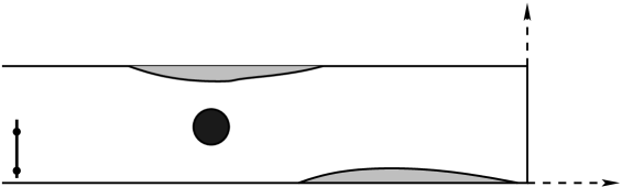
Fig. 1: Illustration of the imaging setup in a terminating waveguide. The system of coordinates is $\vec{{{\itbf x}}}=(x,{{\itbf x}}^{\perp})$ with range $x$ measured from the end wall and cross-range ${{\itbf x}}^{\perp}$ in the cross-section $\mathfrak{X}$ of the waveguide. The wall deformation of the waveguide is modeled by the boundary $\Gamma$ of the domain $\mathcal{D}$ drawn in gray. A localized scatterer supported in $\Omega$ is drawn in black. The array of sensors lies in the set $\mathcal{A}$. The source and receiver locations are denoted by $\vec{{{\itbf x}}}_{s}$ and $\vec{{{\itbf x}}}_{r}$.

Let us denote by $\mathcal{W}_{o}$ the ideal waveguide with unperturbed walls modeled by the boundary $\partial\mathcal{W}_{o}$, and use the system of coordinates $\vec{{{\itbf x}}}=(x,{{\itbf x}}^{\perp})\in\mathbb{R}^{d}$ shown in Figure 1, with range $x$ measured along the axis of $\mathcal{W}_{o}$, starting from the end wall. The cross-range coordinates ${{\itbf x}}^{\perp}$ lie in the cross-section of $\mathcal{W}_{o}$, denoted by $\mathfrak{X}\subset\mathbb{R}^{d-1}$. This is a compact Lipschitz domain when $d=3$, or an interval of finite length $|\mathfrak{X}|$ when $d=2$. In our system of coordinates we have

$$\mathcal{W}_{o}=(-\infty,0)\times\mathfrak{X},\qquad\partial\mathcal{W}_{o}=\Big{(}(-\infty,0)\times\partial\mathfrak{X}\Big{)}\cup\Big{(}\{0\}\times\mathfrak{X}\Big{)},$$ (1.1)

and we model the unknown waveguide by

$$\mathcal{W}=\mathcal{W}_{o}\cap(\mathbb{R}^{d}\setminus\overline{\mathcal{D}}),$$ (1.2)

where $\mathcal{D}$ is a Lipschitz domain compactly supported in the sector $(-x_{\star},0)\times\mathfrak{X}$ of $\mathcal{W}_{o}$, with part of the boundary $\partial\mathcal{D}$ lying in $\partial\mathcal{W}_{o}$. We denote this part by $\Gamma_{o}$ and model the unknown waveguide walls by

$$\Gamma=\partial\mathcal{D}\setminus\overline{\Gamma}_{o}\subset\mathcal{W}_{o},$$ (1.3)

where the bar denotes the closure of $\Gamma_{o}$. The waveguide is filled with a homogeneous medium (e.g. air) but it may contain one or more impenetrable or penetrable scatterers supported in the compact set $\Omega$, satisfying

$$\Omega\subset\mathcal{W}\cap\Big{(}(-x_{\star},0)\times\mathfrak{X}\Big{)}.$$ (1.4)

This is a Lipschitz domain or the union of a few disjoint such domains.

The imaging problem is to estimate $\Gamma$ and $\Omega$ using data gathered by an array of $J_{{}_{\mathcal{A}}}$ sensors located in the set

$$\mathcal{A}\subseteq\{x_{{}_{\mathcal{A}}}\}\times\mathfrak{X},\quad x_{{}_{\mathcal{A}}}<x_{\star}<0,$$ (1.5)

called the array aperture. The array probes the waveguide by emitting a time harmonic wave from one of the sensors, at location $\vec{{{\itbf x}}}_{s}$, and measures the echoes $u(\vec{{{\itbf x}}}_{r},\vec{{{\itbf x}}}_{s})$ at all the sensors $\{\vec{{{\itbf x}}}_{r}\}_{r=1,\ldots,J_{{}_{\mathcal{A}}}}$. Although $s$ and $r$ are indexes in the set $\{1,\ldots,J_{{}_{\mathcal{A}}}\}$, we use them consistently to distinguish between the source and receiver. The data gathered successively, with one source at a time, form the $J_{{}_{\mathcal{A}}}\times J_{{}_{\mathcal{A}}}$ response matrix $\big{(}u(\vec{{{\itbf x}}}_{r};\vec{{{\itbf x}}}_{s})\big{)}_{1\leq r,s\leq J_{{}_{\mathcal{A}}}}$. The goal is to show with analysis and numerical simulations how the linear sampling approach estimates $\Gamma$ and $\Omega$ from this matrix.

The paper is organized as follows: We begin in Section 2 with the estimation of $\Gamma$. The estimation of both $\Gamma$ and $\Omega$ is considered in Section 3. The assessment with numerical simulations is in Section 4. We end with a summary in section 5.

2 Imaging wall deformations

We define in Section 2.1 the Green’s function in the unperturbed waveguide, which models the incident wave emitted by a source in the array. The model of the scattered wave measured at the array is given in Section 2.2. The linear sampling approach is analyzed in Section 2.3, for the case of a full aperture array. Imaging with a partial aperture array is described in Section 2.4.

2.1 The incident wave field

Let us denote by $G(\vec{{{\itbf x}}},\vec{{{\itbf y}}})$ the Green’s function in the ideal waveguide $\mathcal{W}_{o}$, for an arbitrary source location $\vec{{{\itbf y}}}=(y,{{\itbf y}}^{\perp})\in\mathcal{W}_{o}$. The model of the incident wave emitted by the source at location $\vec{{{\itbf x}}}_{s}\in\mathcal{A}$ is then

$$u^{{\rm inc}}(\vec{{{\itbf x}}},\vec{{{\itbf x}}}_{s})=G(\vec{{{\itbf x}}},\vec{{{\itbf x}}}_{s}).$$ (2.6)

The Green’s function satisfies the Helmholtz equation

$$\big{(}\Delta_{\vec{{{\itbf x}}}}+k^{2}\big{)}G(\vec{{{\itbf x}}},\vec{{{\itbf y}}})=-\delta(\vec{{{\itbf x}}}-\vec{{{\itbf y}}}),\quad\vec{{{\itbf x}}}\in\mathcal{W}_{o},$$ (2.7)

where $\Delta_{\vec{{{\itbf x}}}}$ is the Laplacian with respect to $\vec{{{\itbf x}}}$ and $k$ is the wavenumber. At the sound hard walls $\partial\mathcal{W}_{o}$ we have the boundary condition

$$\frac{\partial G(\vec{{{\itbf x}}},\vec{{{\itbf y}}})}{\partial\vec{\bm{\nu}}_{{}_{\vec{{{\itbf x}}}}}}=0,\quad\vec{{{\itbf x}}}\in\partial W_{o},$$ (2.8)

where $\vec{\bm{\nu}}_{{}_{\vec{{{\itbf x}}}}}$ denotes the outer unit normal at $\vec{{{\itbf x}}}$, and for $\vec{{{\itbf x}}}\in\mathcal{W}_{o}$ with range coordinate $x<y$ we impose the radiation condition formulated precisely in Definition 1, which states that $G(\vec{{{\itbf x}}},\vec{{{\itbf y}}})$ is a bounded and outgoing wave.

Due to the simple geometry of $\mathcal{W}_{o}$, the Green’s function can be written explicitly using the eigenfunctions $\{\psi_{j}({{\itbf x}}^{\perp})\}_{j\geq 0}$ of the Laplacian $\Delta_{{{\itbf x}}^{\perp}}$ in $\mathfrak{X}$, satisfying

$$-\Delta_{{{\itbf x}}^{\perp}}\psi_{j}({{\itbf x}}^{\perp}) =\lambda_{j}\psi_{j}({{\itbf x}}^{\perp}),\qquad{{\itbf x}}^{\perp}\in\mathfrak{X},$$

$$\frac{\partial\psi_{j}({{\itbf x}}^{\perp})}{\partial\nu_{{{{\itbf x}}^{\perp}}}} =0,\quad{{\itbf x}}^{\perp}\in\partial\mathfrak{X},$$ (2.9)

where $\nu_{{{{\itbf x}}^{\perp}}}$ is the outer normal at ${{\itbf x}}^{\perp}$, in the plane of $\mathfrak{X}\subset\mathbb{R}^{d-1}$. The spectral theorem for compact self-adjoint linear operators [22, Theorem 2.36] implies that these eigenfunctions form a complete orthonormal basis of $L^{2}(\mathfrak{X})$ and that the eigenvalues $\lambda_{j}$ are real and non-negative. The first eigenvalue $\lambda_{o}=0$ is simple and corresponds to the constant eigenfunction $\psi_{0}({{\itbf x}}^{\perp})={1}/\sqrt{|\mathfrak{X}|}$. The other eigenvalues satisfy

$$0=\lambda_{o}<\lambda_{1}\leq\lambda_{2}\leq\ldots,\qquad\lim_{j\to\infty}\lambda_{j}=\infty.$$ (2.10)

The expression of the Green’s function is

$$G(\vec{{{\itbf x}}},\vec{{{\itbf y}}})=\sum_{j=0}^{\infty}\frac{i}{2\beta_{j}}\psi_{j}({{\itbf y}}^{\perp})\psi_{j}({{\itbf x}}^{\perp})\Big{(}e^{i\beta_{j}|x-y|}+e^{i\beta_{j}|x+y|}\Big{)},$$ (2.11)

where

$$\beta_{j}=\left\{\begin{array}[]{ll}\sqrt{k^{2}-\lambda_{j}},&j=0,1,\ldots,J,\\ \\ i\sqrt{\lambda_{j}-k^{2}},&j>J,\end{array}\right.$$ (2.12)

and $J$ is the largest index $j$ such that $\lambda_{j}\leq k^{2}$.

Note that at points $\vec{{{\itbf x}}}=(x,{{\itbf x}}^{\perp})\in\mathcal{W}_{o}$ between the source at $\vec{{{\itbf y}}}=(y,{{\itbf y}}^{\perp})$ and the end wall i.e., for range $x\in(y,0)$, the expression (2.11) consists of $J+1$ propagating modes $\{\psi_{j}({{\itbf x}}^{\perp})e^{\pm i\beta_{j}x}\}_{0\leq j\leq J}$ and infinitely many growing and decaying (evanescent) modes $\{\psi_{j}({{\itbf x}}^{\perp})e^{\pm\beta_{j}x}\}_{j>J}$ with complex amplitudes that depend on $\vec{{{\itbf y}}}$. The propagating modes can be understood as superpositions of plane waves with wave vector $(\pm\beta_{j},\bm{\kappa}_{j})$, where $\bm{\kappa}_{j}\in\mathbb{R}^{d-1}$ has the square Euclidian norm $\lambda_{j}$. These waves propagate forward and backward in the range direction, at group speed

$$c\Big{(}\frac{d\beta_{j}}{dk}\Big{)}^{-1}=c\frac{\beta_{j}}{k},\qquad j=0,\ldots,J,$$

where $c$ is the wave speed in the homogeneous medium that fills the waveguide. The fastest mode indexed by $j=0$ propagates at speed $c$. The slowest mode corresponds to $j=J$ and we assume that $\lambda_{J}<k^{2}$, so that $\beta_{J}\neq 0$. The wavenumber is imaginary for indexes $j>J$ and the modes grow or decay exponentially in range.

At points $\vec{{{\itbf x}}}$ with range coordinate $x<y$, the expression (2.11) consists of $J+1$ outgoing (backward) propagating modes $\{\psi_{j}({{\itbf x}}^{\perp})e^{-i\beta_{j}x}\}_{0\leq j\leq J}$ and infinitely many decaying (evanescent) modes $\{\psi_{j}({{\itbf x}}^{\perp})e^{\beta_{j}x}\}_{j>J}$. This is the explicit statement of the radiation condition for the Green’s function.

2.2 The array response matrix

The scattered field $u(\vec{{{\itbf x}}},\vec{{{\itbf x}}}_{s})$ due to the incident wave (2.6) is the function in $H_{{\rm loc}}^{1}(\mathcal{W})$ satisfying the Helmholtz equation

$$\big{(}\Delta_{\vec{{{\itbf x}}}}+k^{2}\big{)}u(\vec{{{\itbf x}}},\vec{{{\itbf x}}}_{s})=0,\qquad\vec{{{\itbf x}}}\in\mathcal{W},$$ (2.13)

with the Neumann boundary conditions

$$\frac{\partial u(\vec{{{\itbf x}}},\vec{{{\itbf x}}}_{s})}{\partial\vec{\bm{\nu}}_{{}_{\vec{{{\itbf x}}}}}} =0,\quad\partial W_{o}\setminus\overline{\Gamma}_{o},$$ (2.14)

$$\frac{\partial u(\vec{{{\itbf x}}},\vec{{{\itbf x}}}_{s})}{\partial\vec{\bm{\nu}}_{{}_{\vec{{{\itbf x}}}}}} =-\frac{\partial G(\vec{{{\itbf x}}},\vec{{{\itbf x}}}_{s})}{\partial\vec{\bm{\nu}}_{{}_{\vec{{{\itbf x}}}}}},\qquad\vec{{{\itbf x}}}\in\Gamma,$$ (2.15)

at the sound hard walls, and the radiation condition at points $\vec{{{\itbf x}}}\in\mathcal{W}$ with range coordinate $x<x_{\star}$. Due to the assumption that the wall deformation is supported in the range interval $(x_{\star},0)$, with $x_{{}_{\mathcal{A}}}<x_{\star}$, the radiation condition is as in the previous section:

Definition 1.

The radiation condition at points $\vec{{{\itbf x}}}=(x,{{\itbf x}}^{\perp})\in\mathcal{W}$ with $x<x_{\star}$ means that $u(\vec{{{\itbf x}}},\vec{{{\itbf x}}}_{s})$ is a superposition of $J+1$ backward going modes and infinitely many decaying modes,

$$u(\vec{{{\itbf x}}},\vec{{{\itbf x}}}_{s})=\sum_{j=0}^{\infty}\alpha_{j}(\vec{{{\itbf x}}}_{s},\Gamma)\psi_{j}({{\itbf x}}^{\perp})e^{-i\beta_{j}x},\qquad\vec{{{\itbf x}}}=(x,{{\itbf x}}^{\perp}),~{}~{}x<x_{\star}.$$ (2.16)

Each term (mode) in the sum is a special solution of the Helmoltz equation in the sector $(-\infty,x_{\star})\times\mathfrak{X}$ of $\mathcal{W}$. The complex amplitudes $\alpha_{j}$ depend on $\vec{{{\itbf x}}}_{s}$ and $\Gamma$.

The array is located far from the wall deformation, so the response matrix can be modeled as

$$u(\vec{{{\itbf x}}}_{r},\vec{{{\itbf x}}}_{s})\approx\sum_{j=0}^{J}\alpha_{j}(\vec{{{\itbf x}}}_{s},\Gamma)e^{-i\beta_{j}x_{{}_{\mathcal{A}}}}\psi_{j}({{\itbf x}}^{\perp}_{r}),\qquad\forall\,\vec{{{\itbf x}}}_{r},\vec{{{\itbf x}}}_{s}\in\mathcal{A},$$ (2.17)

where we neglect the evanescent waves.

2.3 The linear sampling approach

In this section we show how to use the linear sampling approach to estimate $\Gamma$ from the array response matrix with entries (2.17). In the analysis we assume that the sensors are located very close together in the array and we replace sums over the sensor indexes by integrals over $\mathcal{A}$. Although we keep the notation $\vec{{{\itbf x}}}_{s}$ and $\vec{{{\itbf x}}}_{r}$ for the source and receiver locations, these are now vectors that vary continuously in $\mathcal{A}$. We begin with the case of full array aperture

$$\mathcal{A}=\{x_{{}_{\mathcal{A}}}\}\times\mathfrak{X},$$ (2.18)

and postpone until the next section the discussion for partial aperture. However we remark that the theoretical justification of the linear sampling method for partial aperture remains unchanged.

2.3.1 Analysis of the linear sampling approach

Let us introduce the so-called near field integral operator $N:L^{2}(\mathcal{A})\to L^{2}(\mathcal{A})$ defined by

$$Ng(\vec{{{\itbf x}}}_{r})=\int_{\mathcal{A}}dS_{\vec{{{\itbf x}}}_{s}}\,u(\vec{{{\itbf x}}}_{r},\vec{{{\itbf x}}}_{s})g(\vec{{{\itbf x}}}_{s}),\qquad\forall g\in L^{2}(\mathcal{A}),~{}~{}\vec{{{\itbf x}}}_{r}\in\mathcal{A},$$ (2.19)

where we note that the assumption (2.18) implies that the cross-range components of $\vec{{{\itbf x}}}_{r},\vec{{{\itbf x}}}_{s}$ lie in $\mathfrak{X}$. By linear superposition, the function $Ng(\vec{{{\itbf x}}}_{r})$ represents the scattered wave received at $\vec{{{\itbf x}}}_{r}$, due to an illumination $g(\vec{{{\itbf x}}}_{s})$ from all the source points $\vec{{{\itbf x}}}_{s}\in\mathcal{A}$. The linear sampling method uses this $g(\vec{{{\itbf x}}}_{s})$ as a control at the array, which focuses the wave at a point $\vec{{{\itbf z}}}$ in the imaging domain, so that the received wave $Ng(\vec{{{\itbf x}}}_{r})$ equals $G(\vec{{{\itbf x}}}_{r},\vec{{{\itbf z}}})$. It turns out that the control function $g$ is not physical (i.e., it is not bounded in $L^{2}(\mathcal{A})$) if $\vec{{{\itbf z}}}\notin\mathcal{D}$, and this leads to the linear sampling imaging approach.

Our analysis of the linear sampling method is based on the following factorization of the near field operator, proved in appendix A:

Lemma 2.

The operator $N$ defined in (2.19) has the factorization

$$N=T^{\Gamma\to\mathcal{A}}T^{\mathcal{A}\to\Gamma},$$ (2.20)

where $T^{\mathcal{A}\to\Gamma}:L^{2}(\mathcal{A})\to H^{-\frac{1}{2}}(\Gamma)$ is the operator

$$T^{\mathcal{A}\to\Gamma}g(\vec{{{\itbf z}}})=\partial_{\vec{\bm{\nu}}_{{}_{\vec{{{\itbf z}}}}}}\int_{\mathcal{A}}dS_{\vec{{{\itbf x}}}_{s}}\,G(\vec{{{\itbf z}}},\vec{{{\itbf x}}}_{s})g(\vec{{{\itbf x}}}_{s}),\qquad\forall g\in L^{2}(\mathcal{A}),~{}\vec{{{\itbf z}}}\in\Gamma,$$ (2.21)

and $T^{\Gamma\to\mathcal{A}}:H^{-\frac{1}{2}}(\Gamma)\to L^{2}(\mathcal{A})$ is the operator defined by the trace $T^{\Gamma\to\mathcal{A}}f=w|_{\mathcal{A}}$ of the solution of

$$\big{(}\Delta_{\vec{{{\itbf x}}}}+k^{2}\big{)}w(\vec{{{\itbf x}}}) =0,\qquad\vec{{{\itbf x}}}\in\mathcal{W},$$ (2.22)

$$\frac{\partial w(\vec{{{\itbf x}}})}{\partial\vec{\bm{\nu}}_{{}_{\vec{{{\itbf x}}}}}} =0,\quad\vec{{{\itbf x}}}\in\partial W_{o}\setminus\overline{\Gamma}_{o},$$ (2.23)

$$\frac{\partial w(\vec{{{\itbf x}}})}{\partial\vec{\bm{\nu}}_{{}_{\vec{{{\itbf x}}}}}} =-f(\vec{{{\itbf x}}}),\qquad\vec{{{\itbf x}}}\in\Gamma,$$ (2.24)

satisfying a radiation condition as in Definition 1.

We conclude from the factorization (2.20) that

$$\mbox{range}\big{(}N\big{)}\subset\mbox{range}\big{(}T^{\Gamma\to\mathcal{A}}\big{)}\subset L^{2}(\mathcal{A}).$$ (2.25)

We also see from (2.22)–(2.24) that the range of $T^{\Gamma\to\mathcal{A}}$ consists of traces on $\mathcal{A}$ of functions that satisfy Helmholtz’s equation in $\mathcal{W}$ with homogeneous Neumann boundary conditions on ${\partial W_{o}\setminus\overline{\Gamma}_{o}}$ and the radiation condition. An example of such a function is $G(\vec{{{\itbf x}}},\vec{{{\itbf z}}})$ for any $\vec{{{\itbf z}}}\in\mathcal{D}$. The next lemma, proved in appendix A, uses this observation to distinguish between points inside and outside $\mathcal{D}$.

Lemma 3.

Let $\vec{{{\itbf z}}}$ be a search point in $\mathcal{W}_{o}$, between the array and the end wall. Then, $\vec{{{\itbf z}}}\in\mathcal{D}$ if and only if $G(\cdot,\vec{{{\itbf z}}})|_{\mathcal{A}}\in\mbox{range}\big{(}T^{\Gamma\to\mathcal{A}}\big{)}$.

Since $T^{\Gamma\to\mathcal{A}}$ is unknown, we cannot determine the support of $\mathcal{D}$ directly from Lemma 3. We only know the near field operator (2.19) with range satisfying (2.25). While $G(\cdot,\vec{{{\itbf z}}})|_{\mathcal{A}}\in\mbox{range}\big{(}T^{\Gamma\to\mathcal{A}}\big{)}$ implies the existence of $f\in H^{-\frac{1}{2}}(\Gamma)$ such that $T^{\Gamma\to\mathcal{A}}f=G(\cdot,\vec{{{\itbf z}}})|_{\mathcal{A}}$, it is not clear that $f$ is in $\mbox{range}\big{(}T^{\mathcal{A}\to\Gamma}\big{)}$. The next lemma, proved in appendix A, shows that $f$ can be approximated arbitrarily well by some $\widetilde{f}\in\mbox{range}\big{(}T^{\mathcal{A}\to\Gamma}\big{)}$ and, furthermore, that $N\widetilde{f}\approx G(\cdot,\vec{{{\itbf z}}})|_{\mathcal{A}}$.

Lemma 4.

The linear operator $T^{\mathcal{A}\to\Gamma}$ is bounded and has dense range in $H^{-\frac{1}{2}}(\Gamma)$. The linear operator $T^{\Gamma\to\mathcal{A}}$ is compact and has dense range in $L^{2}(\mathcal{A})$.

Gathering the results in Lemmas 2–4, we can now prove the following result for the linear sampling approach:

Theorem 5.

Let $\vec{{{\itbf z}}}$ be a search point in $\mathcal{W}_{o}$, between the array and the end wall. For any $\varepsilon>0$ let $g_{\vec{{{\itbf z}}}}^{\varepsilon}\in L^{2}(\mathcal{A})$ satisfy

$$\|Ng_{\vec{{{\itbf z}}}}^{\varepsilon}-G(\cdot,\vec{{{\itbf z}}})\|_{L^{2}(\mathcal{A})}<\varepsilon.$$ (2.26)

(which obviously exists since the range of $N$ is dense in $L^{2}(\mathcal{A})$).

There are two possibilities:

1. If $\vec{{{\itbf z}}}\in\mathcal{D}$, there exists a $g_{\vec{{{\itbf z}}}}^{\varepsilon}$ satisfying (2.26) such that the norm $\|T^{\mathcal{A}\to\Gamma}g_{\vec{{{\itbf z}}}}^{\varepsilon}\|_{H^{-\frac{1}{2}}(\Gamma)}$ remains bounded as $\varepsilon\to 0$.

2. If $\vec{{{\itbf z}}}\notin\mathcal{D}$, for any $g_{\vec{{{\itbf z}}}}^{\varepsilon}$ satisfying (2.26), $\displaystyle\lim_{\varepsilon\to 0}\|T^{\mathcal{A}\to\Gamma}g_{\vec{{{\itbf z}}}}^{\varepsilon}\|_{H^{-\frac{1}{2}}(\Gamma)}=\infty$.

This theorem says that it is possible to estimate the support of $\mathcal{D}$ and therefore the deformed walls $\Gamma$, from the magnitude of $\|T^{\mathcal{A}\to\Gamma}g_{\vec{{{\itbf z}}}}^{\varepsilon}\|_{H^{-\frac{1}{2}}(\Gamma)}$. However, this norm cannot be computed, because we do not know $\Gamma$ and therefore $T^{\mathcal{A}\to\Gamma}$. To obtain an imaging method, we use instead the norm $\|g_{\vec{{{\itbf z}}}}^{\varepsilon}\|_{L^{2}(\mathcal{A})}.$ Recalling from Lemma 4 that $T^{\mathcal{A}\to\Gamma}$ is a bounded linear operator, we have

$$\|g_{\vec{{{\itbf z}}}}^{\varepsilon}\|_{L^{2}(\mathcal{A})}\geq\frac{\|T^{\mathcal{A}\to\Gamma}g_{\vec{{{\itbf z}}}}^{\varepsilon}\|_{H^{-\frac{1}{2}}(\Gamma)}}{\|T^{\mathcal{A}\to\Gamma}\|},$$ (2.27)

so if $z\notin\mathcal{D}$, we conclude from case 2. of Theorem 5 that $\displaystyle\lim_{\varepsilon\to 0}\|g_{\vec{{{\itbf z}}}}^{\varepsilon}\|_{L^{2}(\mathcal{A})}=\infty$. However, if $z\in\mathcal{D}$ we cannot guarantee that $\|g_{\vec{{{\itbf z}}}}^{\varepsilon}\|_{L^{2}(\mathcal{A})}$ remains bounded, because there may be large components of $g_{\vec{{{\itbf z}}}}^{\varepsilon}$ in the null space of $T^{\mathcal{A}\to\Gamma}$. Nevertheless, we can control such components by searching for the minimum norm solution $g_{\vec{{{\itbf z}}}}^{\varepsilon}$ of (2.26) or, similarly, by minimizing $\|Ng-G(\cdot,\vec{{{\itbf z}}})\|_{L^{2}(\mathcal{A})}$ using Tikhonov regularization, as explained in section 2.3.2.

Proof of Theorem 5: Let us begin with case 1., for search point $\vec{{{\itbf z}}}\in\mathcal{D}$. By Lemma 3, we conclude that $\exists\,f_{\vec{{{\itbf z}}}}\in H^{-\frac{1}{2}}(\Gamma)$ such that

$$T^{\Gamma\to\mathcal{A}}f_{\vec{{{\itbf z}}}}(\vec{{{\itbf x}}})=G(\vec{{{\itbf x}}},\vec{{{\itbf z}}})|_{\mathcal{A}}.$$ (2.28)

By Lemma 4, since $\mbox{range}\big{(}{T^{\mathcal{A}\to\Gamma}}\big{)}$ is dense in $H^{-\frac{1}{2}}(\Gamma)$, for any $\varepsilon>0$ there exists $g_{\vec{{{\itbf z}}}}^{\varepsilon}\in L^{2}(\mathcal{A})$ such that

$$\|T^{\mathcal{A}\to\Gamma}g_{\vec{{{\itbf z}}}}^{\varepsilon}-f_{\vec{{{\itbf z}}}}\|_{H^{-\frac{1}{2}}(\Gamma)}<\frac{\varepsilon}{\|T^{\Gamma\to\mathcal{A}}\|},$$ (2.29)

where we used that $T^{\Gamma\to\mathcal{A}}$ is bounded, per Lemma 4. Then, the factorization in Lemma 2 and (2.28) give that this $g_{\vec{{{\itbf z}}}}^{\varepsilon}$ satisfies

$$\|Ng_{\vec{{{\itbf z}}}}^{\varepsilon}-G(\cdot,\vec{{{\itbf z}}})\|_{L^{2}(\mathcal{A})}=\big{\|}T^{\Gamma\to\mathcal{A}}\big{(}T^{\mathcal{A}\to\Gamma}g_{\vec{{{\itbf z}}}}^{\varepsilon}-f_{\vec{{{\itbf z}}}}\big{)}\|_{L^{2}(\mathcal{A})}<\varepsilon.$$ (2.30)

We also have using the triangle inequality in (2.29) that

$$\|T^{\mathcal{A}\to\Gamma}g_{\vec{{{\itbf z}}}}^{\varepsilon}\|_{H^{-\frac{1}{2}}(\Gamma)}\leq\frac{\varepsilon}{\|T^{\Gamma\to\mathcal{A}}\|}+\|f_{\vec{{{\itbf z}}}}\|_{H^{-\frac{1}{2}}(\Gamma)}\to\|f_{\vec{{{\itbf z}}}}\|_{H^{-\frac{1}{2}}(\Gamma)}~{}~{}\mbox{ as }~{}\varepsilon\to 0.$$

This proves case 1. of the theorem.

For case 2., let $\vec{{{\itbf z}}}\notin\mathcal{D}$ and conclude from Lemmma 3 that $\forall f\in H^{-\frac{1}{2}}(\Gamma)$,

$$\|T^{\Gamma\to\mathcal{A}}f-G(\cdot,\vec{{{\itbf z}}})\|_{L^{2}(\mathcal{A})}>0.$$ (2.31)

Nevertheless, since $G(\vec{{{\itbf x}}},\vec{{{\itbf z}}})\in L^{2}(\mathcal{A})$ for $\vec{{{\itbf z}}}\notin\mathcal{A}$ and $\mbox{range}\big{(}T^{\Gamma\to\mathcal{A}}\big{)}$ is dense in $L^{2}(\mathcal{A})$ by Lemma 4, we can construct a sequence $\{f_{n}\}_{n\geq 1}$ in $H^{-\frac{1}{2}}(\Gamma)$ such that

$$\|T^{\Gamma\to\mathcal{A}}f_{n}-G(\cdot,\vec{{{\itbf z}}})\|_{L^{2}(\mathcal{A})}<\frac{1}{n},\qquad n\geq 1.$$ (2.32)

Lemma 4 also states that $\mbox{range}\big{(}{T^{\mathcal{A}\to\Gamma}}\big{)}$ is dense in $H^{-\frac{1}{2}}(\Gamma)$, so we can construct a sequence $\{g_{n}\}_{n\geq 1}$ in $L^{2}(\mathcal{A})$ satisfying

$$\|T^{\mathcal{A}\to\Gamma}g_{n}-f_{n}\|_{H^{-\frac{1}{2}}(\Gamma)}<\frac{1}{n},\qquad n\geq 1.$$ (2.33)

These results, the triangle inequality and Lemma 2 give

$$\|Ng_{n}-G(\cdot,\vec{{{\itbf z}}})\|_{L^{2}(\mathcal{A})} =\|T^{\Gamma\to\mathcal{A}}T^{\mathcal{A}\to\Gamma}g_{n}-G(\cdot,\vec{{{\itbf z}}})\|_{L^{2}(\mathcal{A})}$$

$$\leq\big{\|}T^{\Gamma\to\mathcal{A}}\big{(}T^{\mathcal{A}\to\Gamma}g_{n}-f_{n})\big{\|}_{L^{2}(\mathcal{A})}+\|T^{\Gamma\to\mathcal{A}}f_{n}-G(\cdot,\vec{{{\itbf z}}})\|_{L^{2}(\mathcal{A})}$$

$$<\frac{\|T^{\Gamma\to\mathcal{A}}\|+1}{n}.$$ (2.34)

By the Archimedian property of real numbers, $\forall\,\varepsilon>0$, there exists a natural number $N$ such that $\big{(}\|T^{\Gamma\to\mathcal{A}}\|+1\big{)}/n<\varepsilon$, for all $n>N$, so we have shown that (2.26) holds.

It remains to prove that the sequence $\Big{\{}\|T^{\mathcal{A}\to\Gamma}g_{n}\|_{H^{-\frac{1}{2}}(\Gamma)}\Big{\}}_{n\geq 1}$ cannot be bounded. We argue by contradiction: Suppose that this sequence were bounded. Then, we obtain from (2.33) that $\{\|f_{n}\|_{H^{-\frac{1}{2}}(\Gamma)}\}_{n\geq 1}$ is a bounded sequence, so there exists a subsequence $\{f_{n_{m}}\}_{m\geq 1}$ that converges weakly to some $f\in H^{-\frac{1}{2}}(\Gamma)$. By (2.33) this means

$$T^{\mathcal{A}\to\Gamma}g_{n_{m}}\to f,\qquad\mbox{weakly in }H^{-\frac{1}{2}}(\Gamma),$$ (2.35)

and since $T^{\Gamma\to\mathcal{A}}$ is compact by Lemma 4, we have

$$Ng_{n_{m}}=T^{\Gamma\to\mathcal{A}}T^{\mathcal{A}\to\Gamma}g_{n_{m}}\to T^{\Gamma\to\mathcal{A}}f,\qquad\mbox{strongly in }L^{2}(\mathcal{A}).$$ (2.36)

But (2.32) implies that $T^{\Gamma\to\mathcal{A}}f=G(\cdot,\vec{{{\itbf z}}})\big{|}_{\mathcal{A}}$, which contradicts (2.31). This proves that the sequence $\Big{\{}\|T^{\mathcal{A}\to\Gamma}g_{n}\|_{H^{-\frac{1}{2}}(\Gamma)}\Big{\}}_{n\geq 1}$ cannot be bounded, as stated in the theorem.

Remark 1.

The statement of Theorem 5, which is based on the validity of Lemmas 2–4, holds for any wave number $k\in\mathbb{R}$ with the exception of a discrete set of isolated values. These exceptional points correspond to either $-k^{2}$ being a Neuman eigenvalue of the Laplacian in $\mathcal{D}$ or to values of $k^{2}$ at which the forward problem (2.13)–(2.16) is not uniquely solvable. More details are in appendix A.

2.3.2 The imaging algorithm

Suppose that the imaging region is the sector $(x_{{}_{I}},0)\times\mathfrak{X}$ of $\mathcal{W}_{o}$, with $x_{{}_{I}}>x_{{}_{\mathcal{A}}}$ satisfying

$$x_{{}_{I}}-x_{{}_{\mathcal{A}}}>\frac{1}{|\beta_{J+1}|},$$ (2.37)

so that we can neglect all the evanescent modes. Using the mode decomposition of the scattered wave, we can rewrite (2.26) as a linear least squares problem for a $(J+1)\times(J+1)$ linear system of equations. Indeed, by linear superposition, we can decompose the scattered field as

$$u(\vec{{{\itbf x}}}_{r},\vec{{{\itbf x}}}_{s})=\sum_{j=0}^{\infty}u_{j}(\vec{{{\itbf x}}}_{r})\psi_{j}({{\itbf x}}^{\perp}_{s}),$$ (2.38)

where $u_{j}(\vec{{{\itbf x}}})$ solves (2.13)–(2.16), with $G(\vec{{{\itbf x}}},\vec{{{\itbf x}}}_{s})$ replaced in (2.15) by

$$G_{j}(\vec{{{\itbf x}}})=\int_{\mathfrak{X}}d{{\itbf x}}^{\perp}_{s}\,G(\vec{{{\itbf x}}},\vec{{{\itbf x}}}_{s})\psi_{j}({{\itbf x}}^{\perp}_{s}).$$

Furthermore, we can represent the array response (2.17) by the $(J+1)\times(J+1)$ matrix ${\bf U}=\big{(}U_{j,j^{\prime}}\big{)}_{0\leq j\leq J}$ with entries

$$U_{j,j^{\prime}}=\int_{\mathfrak{X}}d{{\itbf x}}^{\perp}_{r}\int_{\mathfrak{X}}d{{\itbf x}}^{\perp}_{s}\,u(\vec{{{\itbf x}}}_{s},\vec{{{\itbf x}}}_{r})\psi_{j}({{\itbf x}}^{\perp}_{r})\psi_{j^{\prime}}({{\itbf x}}^{\perp}_{s}),$$ (2.39)

where we recall the assumption (2.18).

Neglecting the evanescent modes, we obtain from the definition (2.19) of the near field operator that

$$u(\vec{{{\itbf x}}}_{r},\vec{{{\itbf x}}}_{s})\approx\sum_{j,j^{\prime}=0}^{J}U_{j,j^{\prime}}\psi_{j}({{\itbf x}}^{\perp}_{r})\psi_{j^{\prime}}({{\itbf x}}^{\perp}_{s}),$$ (2.40)

and

$$Ng(\vec{{{\itbf x}}}_{r})\approx\sum_{j=0}^{J}\psi_{j}({{\itbf x}}^{\perp}_{r})\sum_{j^{\prime}=0}^{J}U_{j,j^{\prime}}g_{j^{\prime}}=\sum_{j=0}^{J}\psi_{j}({{\itbf x}}^{\perp}_{r})\big{(}{\bf U}{\bf g}\big{)}_{j},\qquad\forall\,\vec{{{\itbf x}}}_{r}\in\mathcal{A},$$ (2.41)

where ${\bf g}=(g_{o},\ldots,g_{J})^{T}$ is the $J+1$ column vector with components

$$g_{j}=\int_{\mathfrak{X}}d{{\itbf x}}^{\perp}_{s}\,\psi_{j}({{\itbf x}}^{\perp}_{s})g(\vec{{{\itbf x}}}_{s}).$$ (2.42)

Moreover, using the assumption (2.37),

$$G(\vec{{{\itbf x}}}_{r},\vec{{{\itbf z}}})\approx\sum_{j=0}^{J}b_{j,\vec{{{\itbf z}}}}\,\psi_{j}({{\itbf x}}^{\perp}_{r}),$$ (2.43)

with

$$b_{j,\vec{{{\itbf z}}}}=\int_{\mathfrak{X}}d{{\itbf x}}^{\perp}\,\psi_{j}({{\itbf x}}^{\perp})G(\vec{{{\itbf x}}},\vec{{{\itbf z}}}),\qquad\vec{{{\itbf x}}}=(x_{{}_{\mathcal{A}}},{{\itbf x}}^{\perp})\in\mathcal{A}.$$ (2.44)

Letting ${\bf b}_{\vec{{{\itbf z}}}}$ be the $J+1$ column vector with components (2.44), we obtain that

$$Ng(\vec{{{\itbf x}}}_{r})-G(\vec{{{\itbf x}}}_{r},\vec{{{\itbf z}}})\approx\sum_{j=0}^{J}\psi_{j}({{\itbf x}}^{\perp}_{r})\Big{(}{\bf U}{\bf g}-{\bf b}_{\vec{{{\itbf z}}}}\big{)}_{j},\qquad\forall\,\vec{{{\itbf x}}}_{r}\in\mathcal{A}.$$ (2.45)

The eigenfunction are orthonormal, so we can write

$$\|Ng-G(\cdot,\vec{{{\itbf z}}})\|_{L^{2}(\mathcal{A})}\approx\|{\bf U}{\bf g}-{\bf b}_{\vec{{{\itbf z}}}}\|_{2},$$ (2.46)

where $\|\cdot\|_{2}$ is the Euclidian norm. The summary of the linear sampling algorithm for estimating $\Gamma$ is as follows:

Algorithm 6.

Input: The $(J+1)\times(J+1)$ matrix ${\bf U}$ and the imaging mesh.

Processing steps:

1. For a user defined small $\varepsilon>0$, and for all $\vec{{{\itbf z}}}$ on the imaging mesh, solve the normal equations

   $$\big{(}{\bf U}^{\star}{\bf U}+\alpha^{\varepsilon}{\bf I}\big{)}{\bf g}_{\vec{{{\itbf z}}}}={\bf U}^{\star}{\bf b}_{\vec{{{\itbf z}}}},$$ (2.47)

   where ${\bf U}^{\star}$ is the Hermitian adjoint of ${\bf U}$, ${\bf I}$ is the $(J+1)\times(J+1)$ identity matrix and $\alpha^{\varepsilon}$ is a positive Tikhonov regularization parameter chosen according to the Morozov principle, so that

   $$\|{\bf U}{\bf g}_{\vec{{{\itbf z}}}}-{\bf b}_{\vec{{{\itbf z}}}}\|_{2}=\varepsilon\|{\bf g}_{\vec{{{\itbf z}}}}\|_{2}.$$

2. Calculate the indicator function

   $${\cal J}(\vec{{{\itbf z}}})=\frac{1}{\|{\bf g}_{\vec{{{\itbf z}}}}\|_{2}}.$$ (2.48)

Output: The estimate of the support of $\mathcal{D}$ is determined by the set of points $\vec{{{\itbf z}}}$ where ${\cal J}(\vec{{{\itbf z}}})$ exceeds a user defined threshold. The estimated wall deformation $\Gamma$ is the part of the boundary of $\mathcal{D}$ contained in $\mathcal{W}_{o}$.

2.4 Imaging with a partial aperture array

If the array does not cover the entire cross-section of the waveguide,

$$\mathcal{A}=\{x_{{}_{\mathcal{A}}}\}\times\mathfrak{X}_{\mathcal{A}},\qquad\mathfrak{X}_{\mathcal{A}}\subset\mathfrak{X},$$ (2.49)

we can calculate the analogue of (2.39), the $(J+1)\times(J+1)$ matrix ${\bf U}^{\mathcal{A}}=({U}^{\mathcal{A}}_{j,j^{\prime}})_{0\leq j,j^{\prime}\leq J}$ with entries

$$U^{\mathcal{A}}_{j,j^{\prime}}=\int_{\mathfrak{X}_{\mathcal{A}}}d{{\itbf x}}^{\perp}_{r}\int_{\mathfrak{X}_{\mathcal{A}}}d{{\itbf x}}^{\perp}_{s}\,u(\vec{{{\itbf x}}}_{s},\vec{{{\itbf x}}}_{r})\psi_{j}({{\itbf x}}^{\perp}_{r})\psi_{j^{\prime}}({{\itbf x}}^{\perp}_{s}),\qquad j,j^{\prime}=0,\ldots,J.$$ (2.50)

This is related to ${\bf U}$ by

$${\bf U}^{\mathcal{A}}\approx{\bf M}{\bf U}{\bf M},$$ (2.51)

where we used the approximation (2.40) and introduced the symmetric, positive semidefinite Gram matrix ${\bf M}=(M_{j,j^{\prime}})_{0\leq j,j^{\prime}\leq J}$ with entries

$$M_{j,j^{\prime}}=\int_{\mathfrak{X}_{\mathcal{A}}}d{{\itbf x}}^{\perp}\,\psi_{j}({{\itbf x}}^{\perp})\psi_{j^{\prime}}({{\itbf x}}^{\perp}),\qquad j,j^{\prime}=0,\ldots,J.$$ (2.52)

While ${\bf M}$ equals the identity when the array has full aperture, at partial aperture it is poorly conditioned. Thus, we cannot calculate ${\bf U}$ from (2.51) by inverting the Gramian ${\bf M}$. If we let

$${\bf M}={\bf V}\mbox{diag}(\sigma_{0},\ldots,\sigma_{J}){\bf V}^{T},$$ (2.53)

be the eigenvalue decomposition of ${\bf M}$, with ${\bf V}=({{\itbf v}}_{j})_{0\leq j\leq J}$ the orthogonal matrix of eigenvectors ${{\itbf v}}_{j}$, and with the eigenvalues in decreasing order $\sigma_{o}\geq\sigma_{1}\geq\ldots\geq\sigma_{J}\geq 0,$ then we expect that

$$0\leq\sigma_{j}\ll 1,\qquad J_{M}<j\leq J,$$ (2.54)

for some $J_{M}<J$. Then, we approximate ${\bf U}$ by

$$\widetilde{{\bf U}}={\bf M}^{\dagger}{\bf U}^{\mathcal{A}}{\bf M}^{\dagger}\approx{\bf M}^{\dagger}{\bf M}{\bf U}{\bf M}{\bf M}^{\dagger},$$ (2.55)

with

$${\bf M}^{\dagger}={\bf V}\mbox{diag}(\sigma_{0}^{-1},\ldots,\sigma_{J_{M}}^{-1},0,\ldots,0){\bf V}^{T}.$$ (2.56)

Note that ${\bf M}^{\dagger}{\bf M}$ is the orthogonal projection on $\mbox{span}({{\itbf v}}_{o},\ldots,{{\itbf v}}_{J_{M}})$.

The imaging algorithm is almost the same as Algorithm 6, except that the input matrix is replaced by $\widetilde{\bf U}$, which we can compute, and ${\bf b}_{\vec{{{\itbf z}}}}$ is replaced by

$$\widetilde{\bf b}_{\vec{{{\itbf z}}}}={\bf M}^{\dagger}{\bf M}{\bf b}_{\vec{{{\itbf z}}}}.$$ (2.57)

To give a more concrete explanation of the effect of the aperture, let us use definition (2.39) and equation (2.55) to relate $\widetilde{\bf U}$ to the full aperture response

$$\widetilde{\bf U}=\sum_{j,j^{\prime}=0}^{J_{M}}{{\itbf v}}_{j}{{\itbf v}}_{j^{\prime}}^{T}\int_{\mathfrak{X}}d{{\itbf x}}^{\perp}_{r}\,p_{j}({{\itbf x}}^{\perp}_{s})\int_{\mathfrak{X}}d{{\itbf x}}^{\perp}_{s}\,p_{j^{\prime}}({{\itbf x}}^{\perp}_{s})u(\vec{{{\itbf x}}}_{r},\vec{{{\itbf x}}}_{s}),$$ (2.58)

where now $\vec{{{\itbf x}}}_{r},\vec{{{\itbf x}}}_{s}\in\{x_{{}_{\mathcal{A}}}\}\times\mathfrak{X}$ and

$$p_{j}({{\itbf x}}^{\perp})=\sum_{l=0}^{J}v_{l,j}\psi_{l}({{\itbf x}}^{\perp}).$$ (2.59)

The vector (2.57) is

$$\widetilde{\bf b}_{\vec{{{\itbf z}}}}=\sum_{j=0}^{J_{M}}{{\itbf v}}_{j}\int_{\mathfrak{X}}d{{\itbf x}}^{\perp}_{r}\,p_{j}({{\itbf x}}^{\perp}_{r})G\big{(}\vec{{{\itbf x}}}_{r},\vec{{{\itbf z}}}\big{)},$$ (2.60)

and if we use ${\bf g}$ defined in (2.42), we obtain

$$\|\widetilde{\bf U}{\bf g}-\widetilde{\bf b}_{\vec{{{\itbf z}}}}\|_{2}^{2}=\sum_{j=0}^{J_{M}} \left|\int_{\mathfrak{X}}d{{\itbf x}}^{\perp}_{r}p_{j}({{\itbf x}}^{\perp}_{r})\left[\int_{\mathfrak{X}}d{{\itbf x}}^{\perp}_{s}\,u(\vec{{{\itbf x}}}_{r},\vec{{{\itbf x}}}_{s})\widetilde{g}\big{(}\vec{{{\itbf x}}}_{s})-G\big{(}\vec{{{\itbf x}}}_{r},\vec{{{\itbf z}}}\big{)}\right]\right|^{2},$$ (2.61)

with

$$\widetilde{g}(\vec{{{\itbf x}}}_{s})=\sum_{j=0}^{J_{M}}p_{j}({{\itbf y}}^{\perp}){{\itbf v}}_{j}^{T}{\bf g}=\sum_{j=0}^{J_{M}}p_{j}({{\itbf x}}^{\perp}_{s})\int_{\mathfrak{X}}d{{\itbf x}}^{\perp}\,p_{j}({{\itbf x}}^{\perp})g\big{(}(x_{{}_{\mathcal{A}}},{{\itbf x}}^{\perp})\big{)}.$$ (2.62)

We can also define the analogue of (2.40)

$$\widetilde{u}(\vec{{{\itbf x}}},\vec{{{\itbf y}}}) =\sum_{l,l^{\prime}=0}^{J}\widetilde{U}_{l,l^{\prime}}\psi_{l}({{\itbf x}}^{\perp})\psi_{l^{\prime}}({{\itbf y}}^{\perp})$$

$$=\sum_{j,j^{\prime}=0}^{J_{M}}p_{j}({{\itbf x}}^{\perp})p_{j^{\prime}}({{\itbf y}}^{\perp})\int_{\mathfrak{X}}d{{\itbf x}}^{\perp}_{r}\,p_{j}({{\itbf x}}^{\perp})\int_{\mathfrak{X}}d{{\itbf x}}^{\perp}_{s}\,p_{j^{\prime}}({{\itbf x}}^{\perp}_{s})u(\vec{{{\itbf x}}}_{r},\vec{{{\itbf x}}}_{s}),$$ (2.63)

for all $\vec{{{\itbf x}}},\vec{{{\itbf y}}}\in\{x_{{}_{\mathcal{A}}}\}\times\mathfrak{X}.$

Note that $\{p_{j}({{\itbf x}}^{\perp})\}_{0\leq j\leq J}$ is an orthogonal set in $\mbox{span}\{\psi_{j}({{\itbf x}}^{\perp}),~{}0\leq j\leq J\}$, satisfying

$$\int_{\mathfrak{X}}d{{\itbf x}}^{\perp}\,p_{j}({{\itbf x}}^{\perp})p_{j^{\prime}}({{\itbf x}}^{\perp})=\delta_{j,j^{\prime}},\qquad\int_{\mathfrak{X}_{\mathcal{A}}}d{{\itbf x}}^{\perp}\,p_{j}({{\itbf x}}^{\perp})p_{j^{\prime}}({{\itbf x}}^{\perp})=\sigma_{j}\delta_{j,j^{\prime}}.$$ (2.64)

Therefore, $\widetilde{u}$, $\widetilde{\bf b}_{\vec{{{\itbf z}}}}$ and $\widetilde{g}$ are projections of their continuum aperture counterparts on the subspace $\mbox{span}\{p_{j}({{\itbf x}}^{\perp}),~{}0\leq j\leq J_{M}\}$. The second relation in (2.64) shows that $\sigma_{j}\in[0,1]$ and we must have

$$p_{j}({{\itbf x}}^{\perp})\approx 0~{}~{}\mbox{in}~{}\mathfrak{X}_{\mathcal{A}},~{}~{}\mbox{for}~{}~{}j=J_{M}+1,\ldots,J,$$ (2.65)

and

$$p_{j}({{\itbf x}}^{\perp})\approx 0~{}~{}\mbox{in}~{}\mathfrak{X}\setminus\mathfrak{X}_{\mathcal{A}},~{}~{}\mbox{for}~{}~{}\sigma_{j}\approx 1.$$ (2.66)

We verify in the next section, for a two dimensional waveguide, that $\sigma_{j}\approx 1$ for $0<j<J_{M}$, where $J_{M}=\lfloor J{|\mathfrak{X}_{\mathcal{A}}|}/{|\mathfrak{X}|}\rfloor$ and $|\mathfrak{X}_{\mathcal{A}}|$, $|\mathfrak{X}|$ are the lengths of the aperture and cross-section of the waveguide. Thus, the projection limits the support of the functions to the array aperture $\mathcal{A}$.

2.4.1 Illustration in a two dimensional waveguide

In two dimensions, the cross-section of the waveguide is the interval $\mathfrak{X}=(0,|\mathfrak{X}|)$ of length $|\mathfrak{X}|$. Suppose that the array aperture is

$$\mathcal{A}=\{x_{{}_{\mathcal{A}}}\}\times\mathfrak{X}_{\mathcal{A}},\qquad\mathfrak{X}_{\mathcal{A}}=(0,|\mathfrak{X}_{\mathcal{A}}|),\qquad|\mathfrak{X}_{\mathcal{A}}|<|\mathfrak{X}|.$$

Then, using the eigenfunctions (2.9) of the Laplacian

$$\psi_{0}({{\itbf x}}^{\perp})=\frac{1}{\sqrt{|\mathfrak{X}|}},\qquad\psi_{j}({{\itbf x}}^{\perp})=\sqrt{\frac{2}{|\mathfrak{X}|}}\cos\left(\frac{\pi j{{\itbf x}}^{\perp}}{|\mathfrak{X}|}\right),\qquad j\geq 1,$$ (2.67)

we obtain that the Gram matrix ${\bf M}$ is

$$M_{j,j^{\prime}}=\left\{\begin{array}[]{ll}\frac{|\mathfrak{X}_{\mathcal{A}}|}{|\mathfrak{X}|},&j=j^{\prime}=0,\\ \frac{|\mathfrak{X}_{\mathcal{A}}|}{|\mathfrak{X}|}\sqrt{2}\,\mbox{sinc}\left(\pi j^{\prime}\frac{|\mathfrak{X}_{\mathcal{A}}|}{|\mathfrak{X}|}\right),&j=0,~{}1\leq j^{\prime}\leq J,\\ \frac{|\mathfrak{X}_{\mathcal{A}}|}{|\mathfrak{X}|}\sqrt{2}\,\mbox{sinc}\left(\pi j\frac{|\mathfrak{X}_{\mathcal{A}}|}{|\mathfrak{X}|}\right),&j^{\prime}=0,~{}1\leq j\leq J,\\ \frac{|\mathfrak{X}_{\mathcal{A}}|}{|\mathfrak{X}|}\left[\mbox{sinc}\left(\pi(j-j^{\prime})\frac{|\mathfrak{X}_{\mathcal{A}}|}{|\mathfrak{X}|}\right)+\mbox{sinc}\left(\pi(j+j^{\prime})\frac{|\mathfrak{X}_{\mathcal{A}}|}{|\mathfrak{X}|}\right)\right],&1\leq j,j^{\prime},\leq J.\end{array}\right.$$ (2.68)

The eigenvalues of ${\bf M}$ are related to the eigenvalues of the $(2J+1)\times(2J+1)$ prolate matrix [33, 30], which is symmetric and Toeplitz

$${\bf T}=\begin{pmatrix}t_{0}&t_{1}&t_{2}&\ldots&t_{2J}\\ t_{1}&t_{0}&t_{1}&\ldots&t_{2J-1}\\ t_{2}&t_{1}&\ddots&\ddots&\vdots\\ \vdots&&\ddots&\ddots&t_{1}\\ t_{2J}&\ldots&\ldots&t_{1}&t_{0}.\end{pmatrix},\qquad t_{j}=\frac{|\mathfrak{X}_{\mathcal{A}}|}{|\mathfrak{X}|}\mbox{sinc}\left(\pi j\frac{|\mathfrak{X}_{\mathcal{A}}|}{|\mathfrak{X}|}\right).$$ (2.69)

To make the connection to ${\bf M}$, we rewrite ${\bf T}$ as the matrix

$${T}_{j,j^{\prime}}=\frac{|\mathfrak{X}_{\mathcal{A}}|}{|\mathfrak{X}|}\mbox{sinc}\left(\pi(j-j^{\prime})\frac{|\mathfrak{X}_{\mathcal{A}}|}{|\mathfrak{X}|}\right),\qquad-J\leq j,j^{\prime}\leq J,$$ (2.70)

using that $t_{j-j^{\prime}}=T_{j,j^{\prime}}$, for $-J\leq j^{\prime}\leq j\leq J$. This matrix has $J$ odd eigenvectors $\{\bm{\tau}_{j}^{o}\}_{1\leq j\leq J}$ for eigenvalues $\{\sigma_{j}^{o}\}_{1\leq j\leq J}$ and $J+1$ even eigenvectors $\{\bm{\tau}_{j}^{e}\}_{0\leq j\leq J}$ for eigenvalues $\{\sigma_{j}^{e}\}_{0\leq j\leq J}$. Odd and even means that the components $\tau_{l,j}^{o}$ and $\tau_{l,j}^{e}$ of the eigenvectors satisfy

$$\tau_{-l,j}^{o}=-\tau_{l,j}^{o},\qquad\tau_{-l,j}^{e}=\tau_{l,j}^{e},\qquad l=1,\ldots,J.$$

We are interested in the even spectrum of ${\bf T}$, which determines the eigenvalues $\sigma_{j}=\sigma_{j}^{e}$ of ${\bf M}$, with the eigenvectors given by

$${{\itbf v}}_{j}=(v_{0,j},\ldots,v_{J,j})^{T},\qquad v_{l,j}=\left\{\begin{array}[]{ll}\sqrt{2}\,\tau_{0,j}^{e},&l=0\\ \tau_{l,j}^{e},&1\leq l\leq J.\end{array}\right.$$ (2.71)

Then, we conclude from the known properties [30] of the spectrum of ${\bf T}$ that $\sigma_{j}\approx 1$ for $0\leq j<J_{M}=\left\lfloor J\frac{|\mathfrak{X}_{\mathcal{A}}|}{|\mathfrak{X}|}\right\rfloor,$ and that $\sigma_{j}\approx 0$ for $j>J_{M}.$ Moreover, the orthogonal functions $p_{j}({{\itbf x}}^{\perp})$ defined in (2.59) are trigonometric polynomials supported in $\mathfrak{X}_{\mathcal{A}}$ for $0\leq j<J_{M}$ and in $\mathfrak{X}\setminus\mathfrak{X}_{\mathcal{A}}$ for $j>J_{M}$, as stated in the previous section. At the threshold index $j=J_{M}$, the polynomial $p_{J_{M}}({{\itbf x}}^{\perp})$ is sharply peaked at the end of the interval $\mathfrak{X}_{\mathcal{A}}$ [30].

3 Imaging inside the waveguide with wall deformations

The analysis of the linear sampling method for estimating both the support $\Omega$ of scatterers in the waveguide and the wall deformation $\Gamma$ is very similar to that in the previous section, so we do not include it here and state directly the results.

The near field operator is defined as in (2.19), using the scattered wave $u(\vec{{{\itbf x}}}_{r},\vec{{{\itbf x}}}_{s})$ at the array, and its factorization is similar to (2.20)

$$N=T^{\Gamma,\Omega\to\mathcal{A}}T^{\mathcal{A}\to\Gamma,\Omega},$$ (3.72)

where the operators $T^{\Gamma,\Omega\to\mathcal{A}}$ and $T^{\mathcal{A}\to\Gamma,\Omega}$ are the analogues of $T^{\Gamma\to\mathcal{A}}$ and $T^{\mathcal{A}\to\Gamma}$ defined in Lemma 2.

In the case of an impenetrable scatterer, the field $u(\vec{{{\itbf x}}},\vec{{{\itbf x}}}_{s})$ satisfies

$$\big{(}\Delta_{\vec{{{\itbf x}}}}+k^{2}\big{)}u(\vec{{{\itbf x}}},\vec{{{\itbf x}}}_{s}) =0,\qquad\vec{{{\itbf x}}}\in\mathcal{W}\setminus{\overline{\Omega}},$$ (3.73)

$$\frac{\partial u(\vec{{{\itbf x}}},\vec{{{\itbf x}}}_{s})}{\partial\vec{\bm{\nu}}_{{}_{\vec{{{\itbf x}}}}}} =0,\quad\vec{{{\itbf x}}}\in{\partial W_{o}\setminus\overline{\Gamma}_{o}},$$ (3.74)

$$\frac{\partial u(\vec{{{\itbf x}}},\vec{{{\itbf x}}}_{s})}{\partial\vec{\bm{\nu}}_{{}_{\vec{{{\itbf x}}}}}} =-\frac{\partial G(\vec{{{\itbf x}}},\vec{{{\itbf x}}}_{s})}{\partial\vec{\bm{\nu}}_{{}_{\vec{{{\itbf x}}}}}},\qquad\vec{{{\itbf x}}}\in\Gamma,$$ (3.75)

$$\mathcal{B}u(\vec{{{\itbf x}}},\vec{{{\itbf x}}}_{s}) =-\mathcal{B}G(\vec{{{\itbf x}}},\vec{{{\itbf x}}}_{s}),\qquad\vec{{{\itbf x}}}\in\partial\Omega,$$ (3.76)

and the radiation condition in Definition 1, where $\mathcal{B}u=u$ if the scatterer is sound soft and $\mathcal{B}u=\partial_{\vec{\bm{\nu}}_{{}_{\vec{{{\itbf x}}}}}}u$ if it is sound hard (or more generally $\mathcal{B}u$ maybe be a combination of Robin type).

For a penetrable scatterer, modeled by the square $n^{2}(\vec{{{\itbf x}}})$ of the index of refraction, with positive real part $\Re(n^{2})>0$ and non-negative imaginary part $\Im(n^{2})\geq 0$, and with support of $n^{2}(\vec{{{\itbf x}}})-1$ in $\Omega$, the scattered field satisfies

$$\big{(}\Delta_{\vec{{{\itbf x}}}}+k^{2}n^{2}(\vec{{{\itbf x}}})\big{)}u(\vec{{{\itbf x}}},\vec{{{\itbf x}}}_{s}) =-k^{2}\big{(}n^{2}(\vec{{{\itbf x}}})-1)G(\vec{{{\itbf x}}},\vec{{{\itbf x}}}_{s}),\qquad\vec{{{\itbf x}}}\in\mathcal{W},$$ (3.77)

$$\frac{\partial u(\vec{{{\itbf x}}},\vec{{{\itbf x}}}_{s})}{\partial\vec{\bm{\nu}}_{{}_{\vec{{{\itbf x}}}}}} =0,\quad\vec{{{\itbf x}}}\in{\partial W_{o}\setminus\overline{\Gamma}_{o}},$$ (3.78)

$$\frac{\partial u(\vec{{{\itbf x}}},\vec{{{\itbf x}}}_{s})}{\partial\vec{\bm{\nu}}_{{}_{\vec{{{\itbf x}}}}}} =-\frac{\partial G(\vec{{{\itbf x}}},\vec{{{\itbf x}}}_{s})}{\partial\vec{\bm{\nu}}_{{}_{\vec{{{\itbf x}}}}}},\qquad\vec{{{\itbf x}}}\in\Gamma,$$ (3.79)

and the radiation condition in Definition 1.

The operators $T^{\Gamma,\Omega\to\mathcal{A}}$ and $T^{\mathcal{A}\to\Gamma,\Omega}$ are defined as in Lemma 2, with $\Gamma$ replaced by $\Gamma\cup\partial\Omega$, when the scatterer is sound hard.

For a sound soft scatterer we define $T^{\mathcal{A}\to\Gamma,\Omega}:L^{2}(\mathcal{A})\to H^{-\frac{1}{2}}(\Gamma)\times H^{\frac{1}{2}}(\partial\Omega)$ by

$$T^{\mathcal{A}\to\Gamma,\Omega}g(\vec{{{\itbf z}}},\vec{{{\itbf z}}}^{\prime})=\left(\partial_{\vec{\bm{\nu}}_{{}_{\vec{{{\itbf z}}}}}}\int_{\mathcal{A}}dS_{\vec{{{\itbf x}}}_{s}}\,G(\vec{{{\itbf z}}},\vec{{{\itbf x}}}_{s})g(\vec{{{\itbf x}}}_{s}),\int_{\mathcal{A}}dS_{\vec{{{\itbf x}}}_{s}}\,G(\vec{{{\itbf z}}}^{\prime},\vec{{{\itbf x}}}_{s})g(\vec{{{\itbf x}}}_{s})\right),$$ (3.80)

for arbitrary points $\vec{{{\itbf z}}}\in\Gamma$ and $\vec{{{\itbf z}}}^{\prime}\in\partial\Omega$ and for arbitrary $g\in L^{2}(\mathcal{A})$. The operator $T^{\Gamma,\Omega\to\mathcal{A}}:H^{-\frac{1}{2}}(\Gamma)\times H^{\frac{1}{2}}(\partial\Omega)\to L^{2}(\mathcal{A})$ takes arbitrary functions $f_{\Gamma}\in H^{-\frac{1}{2}}(\Gamma)$ and $f_{\partial\Omega}\in H^{\frac{1}{2}}(\partial\Omega)$ and returns the trace $T^{\Gamma,\Omega\to\mathcal{A}}(f_{\Gamma},f_{\partial\Omega})=w\big{|}_{\mathcal{A}}$ of the solution of

$$\big{(}\Delta_{\vec{{{\itbf x}}}}+k^{2}\big{)}w(\vec{{{\itbf x}}}) =0,\qquad\vec{{{\itbf x}}}\in\mathcal{W}\setminus{\overline{\Omega}},$$ (3.81)

$$\frac{\partial w(\vec{{{\itbf x}}})}{\partial\vec{\bm{\nu}}_{{}_{\vec{{{\itbf x}}}}}} =0,\quad\vec{{{\itbf x}}}\in{\partial W_{o}\setminus\overline{\Gamma}_{o}},$$ (3.82)

$$\frac{\partial w(\vec{{{\itbf x}}})}{\partial\vec{\bm{\nu}}_{{}_{\vec{{{\itbf x}}}}}} =-f_{\Gamma}(\vec{{{\itbf x}}}),\qquad\vec{{{\itbf x}}}\in\Gamma,$$ (3.83)

$$w(\vec{{{\itbf x}}}) =-f_{\partial\Omega}(\vec{{{\itbf x}}}),\qquad\vec{{{\itbf x}}}\in\partial\Omega,$$ (3.84)

satisfying the radiation condition as in Definition 1.

For a penetrable scatterer, the operator $T^{\mathcal{A}\to\Gamma,\Omega}:L^{2}(\mathcal{A})\to H^{-\frac{1}{2}}(\Gamma)\times H^{1}(\Omega)$ is

$$T^{\mathcal{A}\to\Gamma,\Omega}g(\vec{{{\itbf z}}},\vec{{{\itbf z}}}^{\prime})=\left(\partial_{\vec{\bm{\nu}}_{{}_{\vec{{{\itbf z}}}}}}\int_{\mathcal{A}}dS_{\vec{{{\itbf x}}}_{s}}\,G(\vec{{{\itbf z}}},\vec{{{\itbf x}}}_{s})g(\vec{{{\itbf x}}}_{s}),\int_{\mathcal{A}}dS_{\vec{{{\itbf x}}}_{s}}\,G(\vec{{{\itbf z}}}^{\prime},\vec{{{\itbf x}}}_{s})g(\vec{{{\itbf x}}}_{s})\right),$$ (3.85)

for arbitrary points $\vec{{{\itbf z}}}\in\Gamma$, $\vec{{{\itbf z}}}^{\prime}\in\Omega$ and functions $g\in L^{2}(\mathcal{A})$. Moreover, the operator $T^{\Gamma,\Omega\to\mathcal{A}}:H^{-\frac{1}{2}}(\Gamma)\times H^{1}(\Omega)\to L^{2}(\mathcal{A})$ is defined by the trace $T^{\Gamma,\Omega\to\mathcal{A}}(f_{\Gamma},f_{\Omega})=w\big{|}_{\mathcal{A}}$ of the solution of the boundary value problem

$$\big{(}\Delta_{\vec{{{\itbf x}}}}+k^{2}n^{2}(\vec{{{\itbf x}}})\big{)}w(\vec{{{\itbf x}}}) =-k^{2}\big{(}n^{2}(\vec{{{\itbf x}}})-1\big{)}f_{\Omega}(\vec{{{\itbf x}}}),\qquad\vec{{{\itbf x}}}\in\mathcal{W},$$ (3.86)

$$\frac{\partial w(\vec{{{\itbf x}}})}{\partial\vec{\bm{\nu}}_{{}_{\vec{{{\itbf x}}}}}} =0,\quad\vec{{{\itbf x}}}\in{\partial W_{o}\setminus\overline{\Gamma}_{o}},$$ (3.87)

$$\frac{\partial w(\vec{{{\itbf x}}})}{\partial\vec{\bm{\nu}}_{{}_{\vec{{{\itbf x}}}}}} =-f_{\Gamma}(\vec{{{\itbf x}}}),\qquad\vec{{{\itbf x}}}\in\Gamma,$$ (3.88)

satisfying a radiation condition as in Definition 1, for arbitrary $f_{\Gamma}\in H^{-\frac{1}{2}}(\Gamma)$ and $f_{\Omega}\in H^{1}(\Omega)$.

The analogue of Theorem 5 is:

Theorem 7.

Let $\vec{{{\itbf z}}}$ be a search point in $\mathcal{W}_{o}$, between the array and the end wall. For any $\varepsilon>0$ let $g_{\vec{{{\itbf z}}}}^{\varepsilon}\in L^{2}(\mathcal{A})$ satisfy

$$\|Ng_{\vec{{{\itbf z}}}}^{\varepsilon}-G(\cdot,\vec{{{\itbf z}}})\|_{L^{2}(\mathcal{A})}<\varepsilon.$$ (3.89)

Let $H$ denote $H^{-\frac{1}{2}}(\Gamma\cup\partial\Omega)$ in the case of a sound hard scatterer, or $H^{-\frac{1}{2}}(\Gamma)\cup H^{\frac{1}{2}}(\partial\Omega)$ for a sound soft scatterer, or $H^{-\frac{1}{2}}(\Gamma)\cup H^{1}(\Omega)$ for a penetrable scatterer. There are two possibilities:

1. If $\vec{{{\itbf z}}}\in\mathcal{D}\cup\Omega$, there exists a $g_{\vec{{{\itbf z}}}}^{\varepsilon}$ satisfying (3.89), such that $\|T^{\mathcal{A}\to\Gamma,\Omega}g_{\vec{{{\itbf z}}}}^{\varepsilon}\|_{H}$ remains bounded as $\varepsilon\to 0$.

2. If $\vec{{{\itbf z}}}\notin\mathcal{D}\cup\Omega$, for any $g_{\vec{{{\itbf z}}}}^{\varepsilon}$ satisfying (3.89), $\displaystyle\lim_{\varepsilon\to 0}\|T^{\mathcal{A}\to\Gamma,\Omega}g_{\vec{{{\itbf z}}}}^{\varepsilon}\|_{H}=\infty$.

Remark 2.

The statement of Theorem 7 also holds for any wave number $k\in\mathbb{R}$ with the exception of a discrete set of isolated values. In this case, in addition to the exceptional wave numbers in Remark 1, one has to exclude the values of $k$ for which $-k^{2}$ is an eigenvalue of the Laplacian in $\Omega$ with the respective boundary condition in the case of impenetrable scatterer or a transmission eigenvalue in $\Omega$ in the case of penetrable scatterer (for the latter see [15]).

As in the previous section, the imaging is based on the indicator function ${1}/{\|{\bf g}_{\vec{{{\itbf z}}}}\|_{2}}$, which is expected to be very small for points $\vec{{{\itbf z}}}\notin\mathcal{D}\cup\Omega$. Algorithm 6 remains unchanged, which is useful because in practice it is not known if the waveguide is empty or not. The case of a partial aperture array is handled the same way as in section 2.4.

4 Numerical results

We assess the performance of the linear sampling algorithm using numerical simulations in a two dimensional waveguide. All the coordinates are scaled by the width $|\mathfrak{X}|$ of the waveguide, and we vary the wavelength to get a smaller or larger number of propagating modes

$$J+1=\left\lfloor k\frac{|\mathfrak{X}|}{\pi}\right\rfloor+1.$$

The array data $u(\vec{{{\itbf x}}}_{r},\vec{{{\itbf x}}}_{s})$ are obtained by solving the wave equation in the sector $(-8|\mathfrak{X}|,0)\times(0,|\mathfrak{X}|)$ of the waveguide, using the high performance multi-physics finite element software Netgen/NGSolve [28] and a perfectly matched layer at the left end of the domain. The separation between the sensors is of the order of the wavelength, more precisely: $\frac{\mathfrak{X}}{25}$ in the case of $10$ and $20$ propagating modes, and $\frac{\mathfrak{X}}{55}$ in the case of $50$ propagating modes. The matrices ${\bf U}$ and ${\bf U}^{\mathcal{A}}$ are calculated as in (2.39) and (2.50), by approximating the integrals with Simpson’s quadrature rule. The data are contaminated with 2% multiplicative noise, meaning that the $ij$-th entry of the contaminated matrix is ${U}_{ij}(1+0.02\delta\ )$ where $\delta$ is a uniformly distributed random number between $0$ and $1$.

The imaging region is $(-4|\mathfrak{X}|,0)\times(0,|\mathfrak{X}|)$ and the array is at range $x_{{}_{\mathcal{A}}}=-5|\mathfrak{X}|$. The images are obtained with Algorithm 6 in the case of a full aperture $\mathcal{A}=\{x_{{}_{\mathcal{A}}}\}\times(0,|\mathfrak{X}|)$ or its modification explained in section 2.4 in the case of partial aperture $\mathcal{A}=\{x_{{}_{\mathcal{A}}}\}\times(0,|\mathfrak{X}_{\mathcal{A}}|)$, with $|\mathfrak{X}_{\mathcal{A}}|<|\mathfrak{X}|$. For better visualization we display the logarithm of the indicator function (2.48).

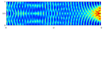
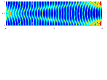
Fig. 2: Reconstruction of wall deformations shown with a solid black line. The abscissa is range and the ordinate is cross-range scaled by $|\mathfrak{X}|$. Full aperture data and $J+1=10$.

The first results, in Fig. 2–4 are obtained with a full aperture. In Fig. 2 we show the reconstruction of wall deformations near the end of the waveguide, for a lower frequency probing wave corresponding to $J+1=10$ propagating modes. The resolution improves at higher frequencies, as illustrated in Fig. 3, where we show reconstructions of wall deformations using $J+1=10$, $20$ and $50$ propagating modes.

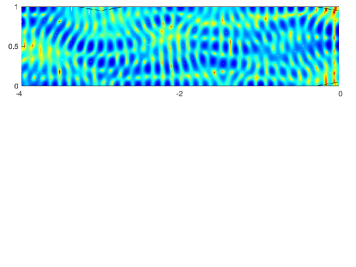
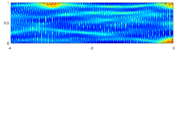
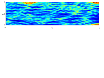
Fig. 3: Reconstruction of wall deformations shown with a solid black line. The abscissa is range and the ordinate is cross-range, scaled by $|\mathfrak{X}|$. Full aperture data and from top to bottom: $J+1=10$, $20$ and $50$.

In Fig. 4 we display images in a waveguide with wall deformations and a scatterer inside. The waveguide supports $50$ propagating modes. The scatterer is impenetrable, with sound soft boundary in the top plot, and it is penetrable in the bottom plot.

The effect of the aperture is illustrated in Fig. 5, in the waveguide considered in the top plot of Fig. 2, but this time the number of propagating modes is increased to $20$. As expected, the image is better for the larger aperture, but even when $|\mathfrak{X}_{\mathcal{A}}|/|\mathfrak{X}|=0.4$, the wall deformation is clearly seen.

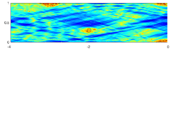
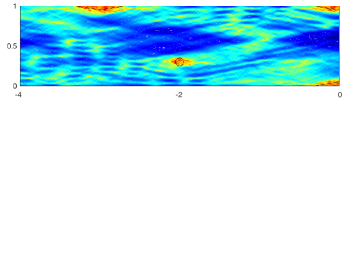
Fig. 4: Reconstruction of wall deformations and a scatterer shown with a solid black line. The abscissa is range and the ordinate is cross-range, scaled by $|\mathfrak{X}|$. Full aperture array data and $J+1=50$. Top: sound-soft scatterer. Bottom: penetrable scatterer.

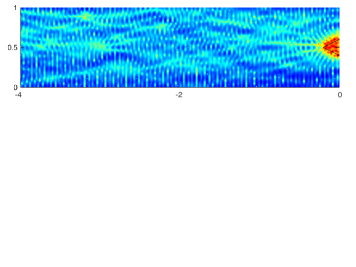
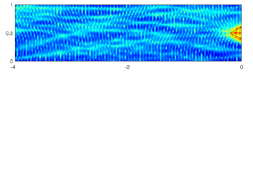
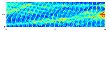
Fig. 5: Reconstruction of wall deformations shown with a solid black line. The abscissa is range and the ordinate is cross-range, scaled by $|\mathfrak{X}|$. Waveguide with $J+1=20$. From top to bottom: $90\%$, $60\%$ and $40\%$ aperture.

5 Summary

We analyzed a direct approach to imaging in a waveguide with reflecting walls and perturbed geometry. The perturbation consists of localized wall deformations that are unknown and are to be determined as part of the imaging. The waveguide may be empty or it may contain some localized, unknown scatterers. The data are gathered by an array of sensors that emits time harmonic probing waves and measures the scattered waves. Ideally, the array spans the entire cross-section of the waveguide, but we also consider partial aperture arrays. Starting from first principles, we established a mathematical foundation of the imaging algorithm. We also assessed its performance using numerical simulations in a two dimensional waveguide.

Appendix A Proofs of Lemmas 2–4

We analyze first in Section A.1 the forward problem (2.13)–(2.16) for the scattered wave field. Then we prove the Lemmas 2–4 in Sections A.2–A.4.

A.1 Forward problem

Let us introduce the truncated waveguide

$$\mathcal{W}_{L}=\mathcal{W}\cap(x_{L},0)\times\mathfrak{X},\qquad x_{L}<x_{{}_{\mathcal{A}}}<0,$$ (A.90)

between the wall at $x=0$ and the truncation boundary

$$\mathcal{L}=\{x_{L}\}\times\mathfrak{X},$$ (A.91)

and show that solving the problem (2.13)–(2.16) in the unbounded $\mathcal{W}$ is equivalent to solving the following boundary value problem in $\mathcal{W}_{L}$:

$$\big{(}\Delta_{\vec{{{\itbf x}}}}+k^{2}\big{)}u(\vec{{{\itbf x}}},\vec{{{\itbf x}}}_{s}) =0,\qquad\vec{{{\itbf x}}}\in\mathcal{W}_{L},$$ (A.92)

$$\frac{\partial u(\vec{{{\itbf x}}},\vec{{{\itbf x}}}_{s})}{\partial\vec{\bm{\nu}}_{{}_{\vec{{{\itbf x}}}}}} =0,\qquad\vec{{{\itbf x}}}\in{\partial\mathcal{W}_{L}\setminus\overline{\Gamma}_{o}},$$ (A.93)

$$\frac{\partial u(\vec{{{\itbf x}}},\vec{{{\itbf x}}}_{s})}{\partial\vec{\bm{\nu}}_{{}_{\vec{{{\itbf x}}}}}} =-\frac{\partial G(\vec{{{\itbf x}}},\vec{{{\itbf x}}}_{s})}{\partial\vec{\bm{\nu}}_{{}_{\vec{{{\itbf x}}}}}},\qquad\vec{{{\itbf x}}}\in\Gamma,$$ (A.94)

$$\frac{\partial u(\vec{{{\itbf x}}},\vec{{{\itbf x}}}_{s})}{\partial\vec{\bm{\nu}}_{{}_{\vec{{{\itbf x}}}}}} =\Lambda_{k}u(\vec{{{\itbf x}}},\vec{{{\itbf x}}}_{s}),\qquad\vec{{{\itbf x}}}\in\mathcal{L}.$$ (A.95)

Here we introduced the Dirichlet to Neumann map

$$\Lambda_{k}:\widehat{H}^{\frac{1}{2}}(\mathcal{L})\to\widehat{H}^{-\frac{1}{2}}(\mathcal{L}),\qquad\Lambda_{k}g(\vec{{{\itbf x}}})\big{|}_{\mathcal{L}}=\sum_{j=0}^{\infty}i\beta_{j}g_{j}\psi_{j}({{\itbf x}}^{\perp}),$$ (A.96)

defined for all $g\in\widehat{H}^{\frac{1}{2}}(\mathcal{L})$, with components

$$g_{j}=\int_{\mathfrak{X}}d{{\itbf x}}^{\perp}\,\psi_{j}({{\itbf x}}^{\perp})g((x_{L},{{\itbf x}}^{\perp})).$$ (A.97)

The subspaces $\widehat{H}^{\frac{m}{2}}(\mathcal{L})$ of $H^{\frac{m}{2}}(\mathcal{L})$ for $m=\pm 1$ correspond to functions that satisfy Neumann boundary conditions,

$$\widehat{H}^{\frac{m}{2}}(\mathcal{L})=\mbox{closure}\Big{\{}v({{\itbf x}}^{\perp})\in\mbox{span}\{\psi_{j}({{\itbf x}}^{\perp}),~{}j\geq 0\}~{}\mbox{s.t.}~{}\sum_{j=0}^{\infty}(1+\lambda_{j})^{\frac{m}{2}}|v_{j}|^{2}<\infty\Big{\}},$$ (A.98)

where

$$v_{j}=\int_{\mathfrak{X}}d{{\itbf x}}^{\perp}\,\psi_{j}({{\itbf x}}^{\perp})v({{\itbf x}}^{\perp}).$$ (A.99)

The norm in $\widehat{H}^{\frac{m}{2}}(\mathcal{L})$ is

$$\|v\|_{\widehat{H}^{\frac{m}{2}}(\mathcal{L})}=\Big{[}\sum_{j=0}^{\infty}(1+\lambda_{j})^{\frac{m}{2}}|v_{j}|^{2}\Big{]}^{\frac{1}{2}}$$ (A.100)

and the duality pairing between $\widehat{H}^{-\frac{m}{2}}(\mathcal{L})$ and $\widehat{H}^{\frac{m}{2}}(\mathcal{L})$ is

$$\left<v,w\right>=\sum_{j=0}^{\infty}v_{j}^{\star}w_{j},\qquad\forall v\in\widehat{H}^{-\frac{m}{2}}(\mathcal{L}),~{}~{}\forall w\in\widehat{H}^{\frac{m}{2}}(\mathcal{L}),$$ (A.101)

where the star denotes complex conjugate.

Lemma 8.

The map $\Lambda_{k}$ is bounded for any $k$. The map $\Lambda_{i}$ is negative definite and the map $\Lambda_{k}-\Lambda_{i}$ is compact.

Proof: We have by the definition (A.96) that

$$\|\Lambda_{k}g\|^{2}_{\widehat{H}^{-\frac{1}{2}}(\mathcal{L})}=\sum_{j=0}^{\infty}(1+\lambda_{j})^{-\frac{1}{2}}|\beta_{j}g_{j}|^{2}=\sum_{j=0}^{\infty}(1+\lambda_{j})^{\frac{1}{2}}|g_{j}|^{2}\frac{|\beta_{j}|^{2}}{1+\lambda_{j}}\leq C\|g\|^{2}_{\widehat{H}^{\frac{1}{2}}(\mathcal{L})},$$

where we used definition (2.12) of $\beta_{j}$ to obtain the bound

$$\frac{|\beta_{j}|^{2}}{1+\lambda_{j}}=\frac{|k^{2}-\lambda_{j}|}{1+\lambda_{j}}\leq C,$$

with constant $C>0$ independent of $j$. This shows that $\Lambda_{k}$ is bounded, for any $k$.

Using the duality pairing (A.101), the definition (2.12) with $k$ replaced by $i$ so that $\beta_{j}$ becomes $i(1+\lambda_{j})^{\frac{1}{2}},$ and

$$\Lambda_{i}g(\vec{{{\itbf x}}})\big{|}_{\mathcal{L}}=-\sum_{j=0}^{\infty}(1+\lambda_{j})^{\frac{1}{2}}g_{j}\psi_{j}({{\itbf x}}^{\perp}),\qquad\forall\,g\in\widehat{H}^{\frac{1}{2}}(\mathcal{L}),$$ (A.102)

we have for all $g\in\widehat{H}^{\frac{1}{2}}(\mathcal{L})$ that

$$\left<\Lambda_{i}g,g\right>=-\sum_{j=0}^{\infty}(1+\lambda_{j})^{\frac{1}{2}}|g_{j}|^{2}=-\|g\|^{2}_{\widehat{H}^{\frac{1}{2}}(\mathcal{L})},$$

so $\Lambda_{i}$ is negative definite.

We also have from (A.96) and (A.102) that

$$(\Lambda_{k}-\Lambda_{i})g(\vec{{{\itbf x}}})\big{|}_{\mathcal{L}}=\sum_{j=0}^{\infty}\big{[}i\beta_{j}+(1+\lambda_{j})^{\frac{1}{2}}\big{]}g_{j}\psi_{j}({{\itbf x}}^{\perp}),\qquad\forall\,g\in\widehat{H}^{\frac{1}{2}}(\mathcal{L}),$$ (A.103)

and we now show that in fact $(\Lambda_{k}-\Lambda_{i})g\in\widehat{H}^{\frac{1}{2}}(\mathcal{L})$. Then, the compact embedding of $\widehat{H}^{\frac{1}{2}}(\mathcal{L})$ in $\widehat{H}^{-\frac{1}{2}}(\mathcal{L})$ gives that $\Lambda_{k}-\Lambda_{i}$ is compact.

Indeed, we have

$$\big{\|}(\Lambda_{k}-\Lambda_{i})g\big{\|}^{2}_{\widehat{H}^{\frac{1}{2}}(\mathcal{L})} =\sum_{j=0}^{\infty}(1+\lambda_{j})^{\frac{1}{2}}\big{|}i\beta_{j}+(1+\lambda_{j})^{\frac{1}{2}}\big{|}^{2}|g_{j}|^{2}$$

$$=\sum_{j=0}^{\infty}(1+\lambda_{j})^{-\frac{1}{2}}|g_{j}|^{2}\left|\Big{(}i\beta_{j}+\sqrt{1+\lambda_{j}}\Big{)}\sqrt{1+\lambda_{j}}\right|^{2}$$

$$\leq C\|g\|^{2}_{\widehat{H}^{-\frac{1}{2}}(\mathcal{L})},$$ (A.104)

for some positive constant $C$, because

$$\Big{|}\Big{(}i\beta_{j}+\sqrt{1+\lambda_{j}}\Big{)}\sqrt{1+\lambda_{j}}\Big{|}\leq C_{1},\qquad 0\leq j\leq J,$$ (A.105)

and

$$\Big{(}i\beta_{j}+\sqrt{1+\lambda_{j}}\Big{)}\sqrt{1+\lambda_{j}} =\Big{(}\sqrt{1+\lambda_{j}}-\sqrt{\lambda_{j}-k^{2}}\Big{)}\sqrt{1+\lambda_{j}}$$

$$=\frac{k^{2}+1}{1+\sqrt{\lambda_{j}-k^{2}}/\sqrt{\lambda_{j}+1}}$$

$$\leq C_{2},\qquad j>J,$$ (A.106)

where $C_{1}$ and $C_{2}$ are positive constants. Thus, (A.104) holds with $C=\max\{C_{1}^{2},C_{2}^{2}\}$.

A.1.1 Connection between the scattering problems in $\mathcal{W}$ and $\mathcal{W}_{L}$

Since problem (2.13)–(2.16) is stated in the infinite domain $\mathcal{W}$ and problem (A.92)–(A.95) is stated in the truncated domain $\mathcal{W}_{L}$, we need the following lemma to make the connection:

Lemma 9.

Consider an arbitrary $f\in\widehat{H}^{\frac{1}{2}}(\mathcal{L})$ with the decomposition

$$f(\vec{{{\itbf x}}})\big{|}_{\mathcal{L}}=\sum_{j=0}^{\infty}f_{j}\psi_{j}({{\itbf x}}^{\perp}).$$ (A.107)

There exists a unique solution $w\in H^{1}_{\rm loc}\big{(}(-\infty,x_{L})\times\mathfrak{X}\big{)}$ of the problem

$$\big{(}\Delta_{\vec{{{\itbf x}}}}+k^{2}\big{)}w(\vec{{{\itbf x}}}) =0,\qquad\vec{{{\itbf x}}}\in(-\infty,x_{L})\times\mathfrak{X},$$ (A.108)

$$\frac{\partial w(\vec{{{\itbf x}}})}{\partial\vec{\bm{\nu}}_{{}_{\vec{{{\itbf x}}}}}} =0,\qquad\vec{{{\itbf x}}}\in(-\infty,x_{L})\times\partial\mathfrak{X}$$ (A.109)

$$w(\vec{{{\itbf x}}}) =f(\vec{{{\itbf x}}}),\qquad\vec{{{\itbf x}}}\in\mathcal{L},$$ (A.110)

that satisfies a radiation condition as in Definition 1.

Proof: From the radiation condition we know that $w$ is an outgoing and bounded wave that has the decomposition

$$w(\vec{{{\itbf x}}})=\sum_{j=0}^{\infty}\gamma_{j}e^{-i\beta_{j}x}\psi_{j}({{\itbf x}}^{\perp}),\qquad\forall\,\vec{{{\itbf x}}}=(x,{{\itbf x}}^{\perp}),~{}~{}x<x_{L},~{}{{\itbf x}}^{\perp}\in\mathfrak{X}.$$ (A.111)

This is a solution of (A.108)–(A.110) if

$$\gamma_{j}=f_{j}e^{i\beta_{j}x_{L}},\qquad j\geq 0,$$ (A.112)

so the expression (A.111) becomes

$$w(\vec{{{\itbf x}}})=\sum_{j=0}^{\infty}f_{j}e^{-i\beta_{j}(x-x_{L})}\psi_{j}({{\itbf x}}^{\perp}).$$ (A.113)

Let us check that this is a function in $H^{1}_{\rm loc}\big{(}(-\infty,x_{L})\times\mathfrak{X}\big{)}$.

We have, for any $\xi<x_{L}$, by the orthonormality of the eigenbasis $\{\psi_{j}\}_{j\geq 0}$ that

$$\|w\|^{2}_{\big{(}(-\xi,x_{L})\times\mathfrak{X}\big{)}} =\int_{\xi}^{x_{L}}dx\int_{\mathfrak{X}}d{{\itbf x}}^{\perp}|w(\vec{{{\itbf x}}})|^{2}$$

$$=(x_{L}-\xi)\sum_{j=0}^{J}|f_{j}|^{2}+\sum_{j=J+1}^{\infty}|f_{j}|^{2}\int_{\xi}^{x_{L}}dx\,e^{2|\beta_{j}|(x-x_{L})}$$

$$\leq C\sum_{j=0}^{\infty}|f_{j}|^{2}=C\|f\|^{2}_{L^{2}(\mathcal{L})}\leq C\|f\|_{\widehat{H}^{\frac{1}{2}}(\mathcal{L})}^{2},$$ (A.114)

where $C$ is a positive constant that depends on $\xi$. Furthermore, using

$$\nabla_{\vec{{{\itbf x}}}}w(\vec{{{\itbf x}}})=\sum_{j=0}^{\infty}f_{j}e^{-i\beta_{j}(x-x_{L})}\Big{(}-i\beta_{j}\psi_{j}({{\itbf x}}^{\perp}),\nabla\psi_{j}({{\itbf x}}^{\perp})\Big{)},$$ (A.115)

the orthogonality relation

$$\int_{\mathfrak{X}}d{{\itbf x}}^{\perp}\,\nabla\psi_{j}({{\itbf x}}^{\perp})\cdot\nabla\psi_{j^{\prime}}({{\itbf x}}^{\perp})=\lambda_{j}\delta_{j,j^{\prime}},$$

and definition (2.12) of the mode wavenumbers, we obtain

$$\|\nabla_{\vec{{{\itbf x}}}}w\|^{2}_{\big{(}(-\xi,x_{L})\times\mathfrak{X}\big{)}} =\int_{\xi}^{x_{L}}dx\Big{[}\sum_{j=0}^{J}(\beta_{j}^{2}+\lambda_{j})|f_{j}|^{2}+\sum_{j=J+1}^{\infty}(|\beta_{j}|^{2}+\lambda_{j})|f_{j}|^{2}e^{2|\beta_{j}|(x-x_{L})}\Big{]}$$

$$=(x_{L}-\xi)k^{2}\sum_{j=0}^{J}|f_{j}|^{2}+2\sum_{j=J+1}^{\infty}(1+\lambda_{j})^{\frac{1}{2}}|f_{j}|^{2}\frac{\big{[}1-e^{-2|\beta_{j}|(x_{L}-\xi)}\big{]}(\lambda_{j}-\frac{k^{2}}{2})}{\sqrt{(\lambda_{j}-k^{2})(\lambda_{j}+1)}}$$

$$\leq C^{\prime}\|f\|_{\widehat{H}^{\frac{1}{2}}(\mathcal{L})}^{2},$$ (A.116)

for another positive constant $C^{\prime}$ that depends on $\xi$. The bounds (A.114)–(A.116) and $f\in\widehat{H}^{\frac{1}{2}}(\mathcal{L})$ imply that $w\in H^{1}_{\rm loc}\big{(}(-\infty,x_{L})\times\mathfrak{X}\big{)}$.

It remains to prove the uniqueness of the solution. If both $w$ and $w^{\prime}$ were solutions, then $w-w^{\prime}$ would also be a solution, for $f$ replaced by $0$ in (A.95). Then, the estimates (A.114)–(A.116) give that $w-w^{\prime}=0$, so the solution is unique.

Theorem 10.

The scattering problem (2.13)–(2.16) is equivalent to the problem (A.92)–(A.95).

Proof: Suppose that $u\in H^{1}_{\rm{loc}}(\mathcal{W})$ satisfies (2.13)–(2.16). Then, it has the mode expansion

$$u(\vec{{{\itbf x}}},\vec{{{\itbf x}}}_{s})=\sum_{j=0}^{\infty}\alpha_{j}\psi_{j}({{\itbf x}}^{\perp})e^{-i\beta_{j}x},\qquad\forall\,\vec{{{\itbf x}}}\in(-\infty,x_{L})\times\mathfrak{X},$$ (A.117)

where we suppressed the dependence of $\alpha_{j}$ on $\vec{{{\itbf x}}}_{s}$ in the notation. We conclude that

$$u(\vec{{{\itbf x}}},\vec{{{\itbf x}}}_{s})\big{|}_{\mathcal{L}}=\sum_{j=0}^{\infty}\alpha_{j}\psi_{j}({{\itbf x}}^{\perp})e^{-i\beta_{j}x_{L}}$$ (A.118)

is in $\widehat{H}^{\frac{1}{2}}(\mathcal{L})$ and using definition (A.96),

$$\Lambda_{k}u(\vec{{{\itbf x}}},\vec{{{\itbf x}}}_{s})\big{|}_{\mathcal{L}}=-\partial_{x_{L}}u(\vec{{{\itbf x}}},\vec{{{\itbf x}}}_{s})\big{|}_{\mathcal{L}}=\sum_{j=0}^{\infty}i\beta_{j}\alpha_{j}\psi_{j}({{\itbf x}}^{\perp})e^{-i\beta_{j}x_{L}},$$ (A.119)

as in (A.95). Thus, $u$ satisfies (A.92)–(A.95).

Conversely, if $u\in H^{1}_{\rm{loc}}(\mathcal{W}_{L})$ solves (A.92)–(A.95), we can extend it to $(-\infty,x_{L})\times\mathfrak{X}$ using the Dirichlet to Neumann map (A.96) which is defined taking into consideration the radiation condition.

A.1.2 Variational formulation and Fredholm alternative

Let $v\in H^{1}(\mathcal{W}_{L})$ be arbitrary. Multiplying equation (A.92) by its complex conjugate $v^{\star}$, integrating by parts and using the boundary conditions (A.93)–(A.95), we obtain

$$\int_{\mathcal{W}_{L}}d\vec{{{\itbf x}}}\,\Big{[}\nabla_{\vec{{{\itbf x}}}}u(\vec{{{\itbf x}}},\vec{{{\itbf x}}}_{s})\cdot\nabla_{\vec{{{\itbf x}}}}v^{\star}(\vec{{{\itbf x}}})-k^{2}u(\vec{{{\itbf x}}},\vec{{{\itbf x}}}_{s})v^{\star}(\vec{{{\itbf x}}})\Big{]}-\int_{\mathcal{L}}dS_{\vec{{{\itbf x}}}}v^{\star}(\vec{{{\itbf x}}})\Lambda_{i}w(\vec{{{\itbf x}}})$$

$$=-\int_{\Gamma}dS_{\vec{{{\itbf x}}}}\frac{\partial G(\vec{{{\itbf x}}},\vec{{{\itbf x}}}_{s})}{\partial\vec{\bm{\nu}}_{{}_{\vec{{{\itbf x}}}}}}v^{\star}(\vec{{{\itbf x}}}).$$

Now let us introduce the sesquilinear forms $a(\cdot,\cdot)$ and $h(\cdot,\cdot)$ on $H^{1}(\mathcal{W}_{L})\times H^{1}(\mathcal{W}_{L})$ and the antilinear form $\ell(\cdot)$ on $H^{1}(\mathcal{W}_{L})$, defined by

$$a(w,v) =\int_{\mathcal{W}_{L}}d\vec{{{\itbf x}}}\,\Big{[}\nabla_{\vec{{{\itbf x}}}}w(\vec{{{\itbf x}}})\cdot\nabla_{\vec{{{\itbf x}}}}v^{\star}(\vec{{{\itbf x}}})+w(\vec{{{\itbf x}}})v^{\star}(\vec{{{\itbf x}}})\Big{]}-\int_{\mathcal{L}}dS_{\vec{{{\itbf x}}}}v^{\star}(\vec{{{\itbf x}}})\Lambda_{i}w(\vec{{{\itbf x}}}),$$

$$h(w,v) =-(k^{2}+1)\int_{\mathcal{W}_{L}}d\vec{{{\itbf x}}}\,w(\vec{{{\itbf x}}})v^{\star}(\vec{{{\itbf x}}})-\int_{\mathcal{L}}dS_{\vec{{{\itbf x}}}}v^{\star}(\vec{{{\itbf x}}})(\Lambda_{k}-\Lambda_{i})w(\vec{{{\itbf x}}}),$$

$$\ell(v) =-\int_{\Gamma}dS_{\vec{{{\itbf x}}}}\frac{\partial G(\vec{{{\itbf x}}},\vec{{{\itbf x}}}_{s})}{\partial\vec{\bm{\nu}}_{{}_{\vec{{{\itbf x}}}}}}v^{\star}(\vec{{{\itbf x}}}),\qquad\forall\,w,v\in H^{1}(\mathcal{W}_{L}).$$

The variational formulation of (A.92)–(A.95) is: Find $u(\cdot,\vec{{{\itbf x}}}_{s})\in H^{1}(\mathcal{W}_{L})$ such that

$$a\big{(}u(\cdot,\vec{{{\itbf x}}}_{s}),v)+h\big{(}u(\cdot,\vec{{{\itbf x}}}_{s}),v)=\ell(v),\qquad\forall\,v\in H^{1}(\mathcal{W}_{L}).$$ (A.120)

From Lemma 8 we know that $\Lambda_{i}$ is negative definite, so it is easy to see that $a(\cdot,\cdot)$ is coercive. We also know from Lemma 8 that $\Lambda_{k}-\Lambda_{i}$ is compact, so $h(\cdot,\cdot)$ introduces a compact perturbation of $a(\cdot,\cdot)$. By Fredholm’s alternative, the solvability of (A.120) is equivalent to the uniqueness of the solution. Moreover, we have continuous dependence of $u$ on the incident field at $\Gamma$.

Theorem 11.

Let $k\in\mathbb{R}$ be a positive wavenumber such that

$$\big{(}\Delta_{\vec{{{\itbf x}}}}+k^{2}\big{)}w(\vec{{{\itbf x}}}) =0,\qquad\vec{{{\itbf x}}}\in\mathcal{W}_{L},$$ (A.121)

$$\frac{\partial w(\vec{{{\itbf x}}})}{\partial\vec{\bm{\nu}}_{{}_{\vec{{{\itbf x}}}}}} =0,\qquad\vec{{{\itbf x}}}\in{\partial\mathcal{W}_{L}\setminus\overline{\mathcal{L}}},$$ (A.122)

$$\frac{\partial w(\vec{{{\itbf x}}})}{\partial\vec{\bm{\nu}}_{{}_{\vec{{{\itbf x}}}}}} =\Lambda_{k}w(\vec{{{\itbf x}}}),\qquad\vec{{{\itbf x}}}\in\mathcal{L}=\{x_{L}\}\times\mathfrak{X},$$ (A.123)

has only the trivial solution $w=0$ in $H^{1}(\mathcal{W}_{L})$. Then, there is a unique solution to (A.92)–(A.95), and by Theorem 10 to (2.13)–(2.16), and it satisfies

$$\|u(\cdot,\vec{{{\itbf x}}}_{s})\|_{H^{1}(\mathcal{W}_{L})}\leq C_{L}\left\|\frac{\partial G(\cdot,\vec{{{\itbf x}}}_{s})}{\partial\vec{\bm{\nu}}_{{}_{\vec{{{\itbf x}}}}}}\right\|_{H^{-\frac{1}{2}}(\Gamma)},$$ (A.124)

where $C_{L}$ is a positive constant that depends on $x_{L}$.

A.2 Proof of Lemma 2

Now that we proved the solvability of the forward problem (2.13)–(2.16), we can use the definition of $T^{\Gamma\to\mathcal{A}}$ in Lemma 2 to write

$$u(\vec{{{\itbf x}}}_{r},\vec{{{\itbf x}}}_{s})=\left[T^{\Gamma\to\mathcal{A}}\frac{\partial G(\cdot,\vec{{{\itbf x}}}_{s})}{\partial\vec{\bm{\nu}}_{{}_{\vec{{{\itbf x}}}}}}\Big{|}_{\Gamma}\right](\vec{{{\itbf x}}}_{r}),\qquad\vec{{{\itbf x}}}_{r}\in\mathcal{A}.$$ (A.125)

Substituting in the expression (2.19) of $N$ we get

$$Ng(\vec{{{\itbf x}}}_{r})=\int_{\mathcal{A}}dS_{\vec{{{\itbf x}}}_{s}}\left[T^{\Gamma\to\mathcal{A}}\frac{\partial G(\cdot,\vec{{{\itbf x}}}_{s})}{\partial\vec{\bm{\nu}}_{{}_{\vec{{{\itbf x}}}}}}\Big{|}_{\Gamma}\right](\vec{{{\itbf x}}}_{r})g(\vec{{{\itbf x}}}_{s}),\qquad\forall\,g\in L^{2}(\mathcal{A}).$$ (A.126)

The integrand is smooth, so we can pull out of the integral $T^{\Gamma\to\mathcal{A}}$ and the normal derivative and obtain

$$Ng(\vec{{{\itbf x}}}_{r})=T^{\Gamma\to\mathcal{A}}\left[\partial\vec{\bm{\nu}}_{{}_{\vec{{{\itbf x}}}}}\int_{\mathcal{A}}dS_{\vec{{{\itbf x}}}_{s}}G(\cdot,\vec{{{\itbf x}}}_{s})\Big{|}_{\Gamma}g(\vec{{{\itbf x}}}_{s})\right](\vec{{{\itbf x}}}_{r})=T^{\Gamma\to\mathcal{A}}T^{\mathcal{A}\to\Gamma}g(\vec{{{\itbf x}}}_{r}),$$ (A.127)

where we used the definition of $T^{\mathcal{A}\to\Gamma}$ in Lemma 2.

A.3 Proof of Lemma 3

Suppose first that $\vec{{{\itbf z}}}\in\mathcal{D}$ and let $w(\vec{{{\itbf x}}})$ satisfy (2.22)–(2.24) with

$$f(\vec{{{\itbf x}}})=-\frac{\partial G(\vec{{{\itbf x}}},\vec{{{\itbf z}}})}{\partial\vec{\bm{\nu}}_{{}_{\vec{{{\itbf x}}}}}},\qquad\vec{{{\itbf x}}}\in\Gamma,$$

and the radiation condition as in Definition 1. Then,

$$v(\vec{{{\itbf x}}})=w(\vec{{{\itbf x}}})-G(\vec{{{\itbf x}}},\vec{{{\itbf z}}})$$

solves (2.22)–(2.24) with $f=0$. By Theorem 11, this means that $v=0$ so taking its trace on $\mathcal{A}$ we get

$$v(\vec{{{\itbf x}}})=0=w(\vec{{{\itbf x}}})-G(\vec{{{\itbf x}}},\vec{{{\itbf z}}}),\quad\vec{{{\itbf x}}}\in\mathcal{A}.$$

But $w\big{|}_{\mathcal{A}}=T^{\Gamma\to\mathcal{A}}f$, so we have shown that

$$T^{\Gamma\to\mathcal{A}}f(\vec{{{\itbf x}}})=G(\vec{{{\itbf x}}},\vec{{{\itbf z}}}),\qquad\vec{{{\itbf x}}}\in\mathcal{A},$$

or, equivalently, that $G(\vec{{{\itbf x}}},\vec{{{\itbf z}}})\big{|}_{\mathcal{A}}\in\mbox{range}(T^{\Gamma\to\mathcal{A}})$.

Now let $\vec{{{\itbf z}}}\notin\mathcal{D}$ and suppose for a contradiction argument that $G(\vec{{{\itbf x}}},\vec{{{\itbf z}}})\big{|}_{\mathcal{A}}$ is in $\mbox{range}(T^{\Gamma\to\mathcal{A}})$. Then, there must exist $f\in H^{-\frac{1}{2}}(\Gamma)$ such that

$$T^{\Gamma\to\mathcal{A}}f(\vec{{{\itbf x}}})=w(\vec{{{\itbf x}}})=G(\vec{{{\itbf x}}},\vec{{{\itbf z}}}),\qquad\vec{{{\itbf x}}}\in\mathcal{A},$$

where $w(\vec{{{\itbf x}}})$ satisfies (2.22)–(2.24) and the radiation condition. Define

$$v(\vec{{{\itbf x}}})=w(\vec{{{\itbf x}}})-G(\vec{{{\itbf x}}},\vec{{{\itbf z}}})$$

and note that it satisfies

$$\big{(}\Delta_{\vec{{{\itbf x}}}}+k^{2}\big{)}v(\vec{{{\itbf x}}}) =0,\qquad\vec{{{\itbf x}}}\in(-\infty,x_{{}_{\mathcal{A}}})\times\mathfrak{X},$$

$$\frac{\partial v(\vec{{{\itbf x}}})}{\partial\vec{\bm{\nu}}_{{}_{\vec{{{\itbf x}}}}}} =0,\qquad\vec{{{\itbf x}}}\in(-\infty,x_{{}_{\mathcal{A}}})\times\partial\mathfrak{X},$$

$$v(\vec{{{\itbf x}}}) =0,\quad\vec{{{\itbf x}}}\in\mathcal{A},$$

and the radiation condition. This problem is as in Lemma 9, with $f=0$ and $x_{L}$ replaced by $x_{{}_{\mathcal{A}}}$. Thus, it has the unique solution $v=0$ in $H^{1}_{\rm loc}\big{(}(-\infty,x_{{}_{\mathcal{A}}})\times\mathfrak{X}\big{)}$. By unique continuation, we can extend it to $v=0$ in $\mathcal{W}\setminus\{\vec{{{\itbf z}}}\}$. However, this means that $w(\vec{{{\itbf x}}})=G(\vec{{{\itbf x}}},\vec{{{\itbf z}}})$ which contradicts that $w\in H^{1}_{\rm loc}(\mathcal{W}),$ due to the singularity of the Green’s function at $\vec{{{\itbf x}}}=\vec{{{\itbf z}}}\in\mathcal{W}$.

A.4 Proof of Lemma 4

Since $\Gamma$ is only part of the boundary $\partial\mathcal{W}$ and $\partial\mathcal{D}$, we introduce the following Sobolev spaces on $\Gamma$. Suppose that $\Gamma$, $\overline{\Gamma}\cap(\partial\mathcal{D}\backslash\Gamma)$ and $\partial\mathcal{D}\backslash\overline{\Gamma}$ are Lipschitz dissections of the boundary $\partial\mathcal{D}$. Following the notations in [22], with $\mathfrak{D}(\partial\mathcal{D})$ denoting the space of $C^{\infty}(\partial\mathcal{D})$ functions with compact support, let

$$\mathfrak{D}(\Gamma)=\{\phi\in\mathfrak{D}(\partial\mathcal{D}):\,\mbox{supp}~{}\phi\subset\Gamma_{D}\}.$$

Then, we define

$$H^{s}(\Gamma) = \{\phi|_{\Gamma}:\,\phi\in H^{s}(\partial\mathcal{D})\},$$

$$\widetilde{H}^{s}(\Gamma) = \mbox{closure of }\,\,\mathfrak{D}(\Gamma)\,\mbox{ in }\,H^{s}(\partial\mathcal{D}),$$

for $s=\pm\frac{1}{2}$, where the dual of $H^{s}(\Gamma)$ is $\widetilde{H}^{-s}(\Gamma)$.

Let us begin with the proof that $T^{\mathcal{A}\to\Gamma}$ is bounded. Because $G(\vec{{{\itbf x}}},\vec{{{\itbf x}}}_{s})$ is smooth for $\vec{{{\itbf x}}}\notin\mathcal{A}$, we have that

$$v(\vec{{{\itbf x}}})=\int_{\mathcal{A}}dS_{\vec{{{\itbf x}}}_{s}}G(\vec{{{\itbf x}}},\vec{{{\itbf x}}}_{s})g(\vec{{{\itbf x}}}_{s}),\qquad\forall g\in L^{2}(\mathcal{A}),$$

is in $H^{1}\big{(}(x_{{}_{\mathcal{A}}},0)\times\mathfrak{X}\big{)}$. Moreover,

$$\Delta_{\vec{{{\itbf x}}}}v(\vec{{{\itbf x}}})=\int_{\mathcal{A}}dS_{\vec{{{\itbf x}}}_{s}}\Delta_{\vec{{{\itbf x}}}}G(\vec{{{\itbf x}}},\vec{{{\itbf x}}}_{s})g(\vec{{{\itbf x}}}_{s})=-k^{2}\int_{\mathcal{A}}dS_{\vec{{{\itbf x}}}_{s}}G(\vec{{{\itbf x}}},\vec{{{\itbf x}}}_{s})g(\vec{{{\itbf x}}}_{s}),$$

so we can bound

$$|\Delta_{\vec{{{\itbf x}}}}v(\vec{{{\itbf x}}})|\leq k^{2}\int_{\mathcal{A}}dS_{\vec{{{\itbf x}}}_{s}}|G(\vec{{{\itbf x}}},\vec{{{\itbf x}}}_{s})g(\vec{{{\itbf x}}}_{s})|\leq C\|g\|_{L^{2}(\mathcal{A})},$$

with some positive constant $C$. Here we used the Cauchy-Schwartz inequality and that $G(\vec{{{\itbf x}}},\vec{{{\itbf x}}}_{s})$ is bounded for $\vec{{{\itbf x}}}\notin\mathcal{A}$. Then, we conclude from [22, Theorem 5.7] or [14, Lemma 4.3] that $T^{\mathcal{A}\to\Gamma}g\in H^{-\frac{1}{2}}(\Gamma)$ and its norm is bounded by the $\|g\|_{L^{2}(\mathcal{A})}$. This shows that the linear operator $T^{\mathcal{A}\to\Gamma}$ is bounded.

To prove that $T^{\mathcal{A}\to\Gamma}$ has dense range in $H^{-\frac{1}{2}}(\Gamma)$, we show that $h\in\widetilde{H}^{\frac{1}{2}}(\Gamma)$ must be zero if

$$(T^{\mathcal{A}\to\Gamma}g,h)=0,\qquad\forall g\in L^{2}(\mathcal{A}),$$

where $(\cdot,\cdot)$ denotes the duality pairing. Indeed if

$$(T^{\mathcal{A}\to\Gamma}g,h)=\int_{\Gamma}dS_{\vec{{{\itbf z}}}}\,h^{\star}(\vec{{{\itbf z}}})\frac{\partial}{\partial\vec{\bm{\nu}}_{{}_{\vec{{{\itbf z}}}}}}\int_{\mathcal{A}}dS_{\vec{{{\itbf x}}}_{s}}G(\vec{{{\itbf z}}},\vec{{{\itbf x}}}_{s})g(\vec{{{\itbf x}}}_{s})=0,$$

for all $g\in L^{2}(\mathcal{A})$ and $h^{\star}$ is the conjugate of $h$, then by the reciprocity relation $G(\vec{{{\itbf z}}},\vec{{{\itbf x}}}_{s})=G(\vec{{{\itbf x}}}_{s},\vec{{{\itbf z}}})$ and Fubini’s theorem we conclude

$$\int_{\Gamma}dS_{\vec{{{\itbf z}}}}\,h^{\star}(\vec{{{\itbf z}}})\frac{\partial G(\vec{{{\itbf x}}}_{s},\vec{{{\itbf z}}})}{\partial\vec{\bm{\nu}}_{{}_{\vec{{{\itbf z}}}}}}=0,\qquad\forall\vec{{{\itbf x}}}_{s}\in\mathcal{A}.$$

Let us define

$$w(\vec{{{\itbf x}}})=\int_{\Gamma}dS_{\vec{{{\itbf z}}}}\,h^{\star}(\vec{{{\itbf z}}})\frac{\partial G(\vec{{{\itbf x}}},\vec{{{\itbf z}}})}{\partial\vec{\bm{\nu}}_{{}_{\vec{{{\itbf z}}}}}},$$

and consider first $\vec{{{\itbf x}}}\in(-\infty,x_{{}_{\mathcal{A}}})\times\mathfrak{X}$. By Lemma 9, with $\mathcal{L}$ replaced by $\mathcal{A}$ and right hand side in (A.110) replaced by $0$, we conclude that $w=0$ in $(-\infty,x_{{}_{\mathcal{A}}})\times\mathfrak{X}$. Then, unique continuation yields that

$$w(\vec{{{\itbf x}}})=\int_{\Gamma}dS_{\vec{{{\itbf z}}}}\,h^{\star}(\vec{{{\itbf z}}})\frac{\partial G(\vec{{{\itbf x}}},\vec{{{\itbf z}}})}{\partial\vec{\bm{\nu}}_{{}_{\vec{{{\itbf z}}}}}}=0,\qquad\forall\vec{{{\itbf x}}}\in\mathcal{W}.$$

Since the Green function $G(\vec{{{\itbf x}}},\vec{{{\itbf z}}})$ has the same regularity properties as the Green function for free space [12], by the continuity of the double-layer potential [22] we conclude that $w$ satisfies

$$\Delta_{\vec{{{\itbf x}}}}w(\vec{{{\itbf x}}})+k^{2}w(\vec{{{\itbf x}}}) =0,\qquad\vec{{{\itbf x}}}\in\mathcal{D},$$

$$\frac{\partial w(\vec{{{\itbf x}}})}{\partial\vec{\bm{\nu}}_{{}_{\vec{{{\itbf x}}}}}} =0,\qquad\vec{{{\itbf x}}}\in\partial\mathcal{D},$$

Assuming that $-k^{2}$ is not an eigenvalue of the Laplacian in $\mathcal{D}$, we conclude that $w=0$ in $D$. Then, from the jump relations for double-layer potentials (see for instance [22])

$$h^{\star}(\vec{{{\itbf z}}})=w^{+}(\vec{{{\itbf z}}})-w^{-}(\vec{{{\itbf z}}})=0,\qquad\forall\,\vec{{{\itbf z}}}\in\Gamma.$$

This concludes the proof that $T^{\mathcal{A}\to\Gamma}$ has dense range in $H^{-\frac{1}{2}}(\Gamma)$.

Now let us study the operator $T^{\Gamma\to\mathcal{A}}$ defined in Lemma 2. For all $g\in\widetilde{H}^{\frac{1}{2}}(\Gamma)$ let

$$w_{g}(\vec{{{\itbf x}}})=\int_{\Gamma}dS_{\vec{{{\itbf z}}}}\,\frac{\partial G(\vec{{{\itbf x}}},\vec{{{\itbf z}}})}{\partial\vec{\bm{\nu}}_{{}_{\vec{{{\itbf z}}}}}}g(\vec{{{\itbf z}}}),\qquad\vec{{{\itbf x}}}\in\mathcal{W},$$

and use the jump relations of double layer potentials to define

$$f_{g}(\vec{{{\itbf x}}})=-\frac{\partial}{\partial\vec{\bm{\nu}}_{{}_{\vec{{{\itbf x}}}}}}\int_{\Gamma}dS_{\vec{{{\itbf z}}}}\,\frac{\partial G(\vec{{{\itbf x}}},\vec{{{\itbf z}}})}{\partial\vec{\bm{\nu}}_{{}_{\vec{{{\itbf z}}}}}}g(\vec{{{\itbf z}}}),\qquad\vec{{{\itbf x}}}\in\Gamma.$$

Since $w_{g}$ satisfies (2.22)–(2.24) and the radiation condition, we can write

$$T^{\Gamma\to\mathcal{A}}f_{g}(\vec{{{\itbf x}}})=w_{g}(\vec{{{\itbf x}}}),\qquad\vec{{{\itbf x}}}\in\mathcal{A}.$$

To prove that $\mbox{range}(T^{\Gamma\to\mathcal{A}})$ is dense in $L^{2}(\mathcal{A})$, we show that $h\in L^{2}(\mathcal{A})$, satisfying

$$(T^{\Gamma\to\mathcal{A}}f_{g},h)=0,\qquad\forall g\in\widetilde{H}^{\frac{1}{2}}(\Gamma),$$

must be zero. Here $(\cdot,\cdot)$ denotes the $L^{2}(\mathcal{A})$ inner product. Indeed, if

$$(T^{\Gamma\to\mathcal{A}}f_{g},h)=\int_{\mathcal{A}}dS_{\vec{{{\itbf x}}}}\,h^{\star}(\vec{{{\itbf x}}})\int_{\Gamma}dS_{\vec{{{\itbf z}}}}\frac{\partial G(\vec{{{\itbf x}}},\vec{{{\itbf z}}})}{\partial\vec{\bm{\nu}}_{{}_{\vec{{{\itbf z}}}}}}g(\vec{{{\itbf z}}})=0,\quad\forall\,g\in\widetilde{H}^{\frac{1}{2}}(\Gamma),$$

then, by the reciprocity relation $G(\vec{{{\itbf x}}},\vec{{{\itbf z}}})=G(\vec{{{\itbf z}}},\vec{{{\itbf x}}})$ and by Fubini’s theorem we have that

$$\int_{\mathcal{A}}dS_{\vec{{{\itbf x}}}}\,h^{\star}(\vec{{{\itbf x}}})\frac{\partial G(\vec{{{\itbf z}}},\vec{{{\itbf x}}})}{\partial\vec{\bm{\nu}}_{{}_{\vec{{{\itbf z}}}}}}=0,\qquad\forall\vec{{{\itbf z}}}\in\Gamma.$$ (A.128)

Let

$$v(\vec{{{\itbf z}}})=\int_{\mathcal{A}}dS_{\vec{{{\itbf x}}}}\,h^{\star}(\vec{{{\itbf x}}})G(\vec{{{\itbf z}}},\vec{{{\itbf x}}}),\qquad\vec{{{\itbf z}}}\in\mathcal{W}\setminus\overline{\mathcal{A}}.$$

Since $\mathcal{A}$ and $\Gamma$ do not intersect, we have from (A.128) that

$$\frac{\partial v(\vec{{{\itbf z}}})}{\partial\vec{\bm{\nu}}_{{}_{\vec{{{\itbf z}}}}}}=0,\qquad\vec{{{\itbf z}}}\in\Gamma.$$

Furthermore, from the definition of the Green’s function,

$$\Delta_{\vec{{{\itbf z}}}}v(\vec{{{\itbf z}}})+k^{2}v(\vec{{{\itbf z}}}) =0,\qquad\vec{{{\itbf z}}}\in\mathcal{D},$$

$$\frac{\partial v(\vec{{{\itbf z}}})}{\partial\vec{\bm{\nu}}_{{}_{\vec{{{\itbf z}}}}}} =0,\qquad\vec{{{\itbf z}}}\in\partial\mathcal{D}.$$

Assuming that $-k^{2}$ is not an eigenvalue of the Lapacian in $\mathcal{D}$, we conclude that $v=0$ in $\mathcal{D}$. Unique continuation yields further that $v=0$ in $\mathcal{W}\cap(x_{{}_{\mathcal{A}}},0)\times\mathfrak{X}$ and from the jump relations of the single-layer potential we get that $v=0$ in $H^{\frac{1}{2}}(\mathcal{A}).$ Then, it follows from Lemma 9 that $v=0\in(-\infty,x_{{}_{\mathcal{A}}})\times\mathfrak{X}$. The function $h$ is obtained from the jump relations for the single layer potentials

$${h}^{\star}(\vec{{{\itbf x}}})=\frac{\partial v^{+}(\vec{{{\itbf x}}})}{\partial\vec{\bm{\nu}}_{{}_{\vec{{{\itbf x}}}}}}-\frac{\partial v^{-}(\vec{{{\itbf x}}})}{\partial\vec{\bm{\nu}}_{{}_{\vec{{{\itbf x}}}}}}=0,\qquad\forall\,\vec{{{\itbf x}}}\in\mathcal{A}.$$

This proves that $T^{\Gamma\to\mathcal{A}}$ has dense range in $L^{2}(\mathcal{A})$.

Finally, from the properties of the solution of (2.22)–(2.24) and the radiation condition we have that

$$\|w|_{\mathcal{A}}\|_{H^{\frac{1}{2}}(\mathcal{A})}=\|T^{\Gamma\to\mathcal{A}}f_{g}\|_{{{H^{\frac{1}{2}}(\mathcal{A})}}}\leq C\|f_{g}\|_{H^{-\frac{1}{2}}(\Gamma)}.$$

The compact embedding of $H^{\frac{1}{2}}(\mathcal{A})$ in $L^{2}(\mathcal{A})$ gives that $T^{\Gamma\to\mathcal{A}}$ is compact.

References

- [1] S Acosta, R Alonso, and L Borcea. Source estimation with incoherent waves in random waveguides. Inverse Problems, 31(3):035013, 2015.
- [2] R Alonso, L Borcea, and J Garnier. Wave propagation in waveguides with random boundaries. Communications in Mathematical Sciences, 11(1):233–267, 2012.
- [3] AB Baggeroer, WA Kuperman, and PN Mikhalevsky. An overview of matched field methods in ocean acoustics. IEEE Journal of Oceanic Engineering, 18(4):401–424, 1993.
- [4] MD Bedford and GA Kennedy. Modeling microwave propagation in natural caves passages. IEEE Transactions on Antennas and Propagation, 62(12):6463–6471, 2014.
- [5] L Borcea and J Garnier. Paraxial coupling of propagating modes in three-dimensional waveguides with random boundaries. Multiscale Modeling & Simulation, 12(2):832–878, 2014.
- [6] L Borcea and J Garnier. Pulse reflection in a random waveguide with a turning point. Multiscale Modeling & Simulation, 15(4):1472–1501, 2017.
- [7] L Borcea and J Garnier. A ghost imaging modality in a random waveguide. arXiv preprint arXiv:1804.00549, 2018.
- [8] L Borcea, J Garnier, and D Wood. Transport of power in random waveguides with turning points. Communications in Mathematical Science, 15(8):2327–2371, 2017.
- [9] L Borcea, L Issa, and C Tsogka. Source localization in random acoustic waveguides. Multiscale Modeling & Simulation, 8(5):1981–2022, 2010.
- [10] L Borcea and DL Nguyen. Imaging with electromagnetic waves in terminating waveguides. Inverse problems and imaging, 10:915–941, 2016.
- [11] L Bourgeois, F Le Louër, and E Lunéville. On the use of lamb modes in the linear sampling method for elastic waveguides. Inverse Problems, 27(5):055001, 2011.
- [12] L Bourgeois and E Lunéville. The linear sampling method in a waveguide: a modal formulation. Inverse problems, 24(1):015018, 2008.
- [13] L Bourgeois and E Lunéville. On the use of the linear sampling method to identify cracks in elastic waveguides. Inverse Problems, 29(2):025017, 2013.
- [14] F Cakoni and D Colton. Qualitative Approach to Inverse Scattering Theory. Springer, 2016.
- [15] F Cakoni, D Colton, and H Haddar. Inverse scattering theory and transmission eigenvalues, volume 88 of CBMS-NSF Regional Conference Series in Applied Mathematics. SIAM, Philadelphia, PA, 2016.
- [16] VK Chillara and CJ Lissenden. Review of nonlinear ultrasonic guided wave nondestructive evaluation: theory, numerics, and experiments. Optical Engineering, 55(1):011002, 2015.
- [17] S Dediu and JR McLaughlin. Recovering inhomogeneities in a waveguide using eigensystem decomposition. Inverse Problems, 22(4):1227, 2006.
- [18] J Garnier and G Papanicolaou. Pulse propagation and time reversal in random waveguides. SIAM Journal on Applied Mathematics, 67(6):1718–1739, 2007.
- [19] C Gomez. Loss of resolution for the time reversal of wave in underwater acoustic random channels. Math. Mod. Meth. App. Sci., 23(11):2065–2210, 2013.
- [20] C Gomez. Wave propagation in underwater acoustic waveguides with rough boundaries. Communications in Mathematical Science, 13:2005–2052, 2015.
- [21] A Haack, J Schreyer, and G Jackel. State-of-the-art of non-destructive testing methods for determining the state of a tunnel lining. Tunnelling and Underground Space Technology incorporating Trenchless Technology Research, 10(4):413–431, 1995.
- [22] W McLean. Strongly elliptic systems and boundary integral equations. Cambridge university press, 2000.
- [23] P Monk and V Selgas. Sampling type methods for an inverse waveguide problem. Inverse Problems and Imaging, 6(4):709–747, 2012.
- [24] P Monk and V Selgas. An inverse acoustic waveguide problem in the time domain. Inverse Problems, 32(5):055001, 2016.
- [25] N Mordant, C Prada, and M Fink. Highly resolved detection and selective focusing in a waveguide using the dort method. The Journal of the Acoustical Society of America, 105(5):2634–2642, 1999.
- [26] FD Philippe, C Prada, J de Rosny, D Clorennec, JG Minonzio, and M Fink. Characterization of an elastic target in a shallow water waveguide by decomposition of the time-reversal operator. The Journal of the Acoustical Society of America, 124(2):779–787, 2008.
- [27] P Rizzo, A Marzani, J Bruck, et al. Ultrasonic guided waves for nondestructive evaluation/structural health monitoring of trusses. Measurement science and technology, 21(4):045701, 2010.
- [28] J Schöberl. Netgen an advancing front 2d/3d-mesh generator based on abstract rules. Computing and visualization in science, 1(1):41–52, 1997.
- [29] T Schultz, D Bowen, G Unger, and RH Lyon. Remote acoustical reconstruction of cave and pipe geometries. The Journal of the Acoustical Society of America, 121(5):3155–3155, 2007.
- [30] D Slepian. Prolate spheroidal wave functions, fourier analysis, and uncertainty—v: The discrete case. Bell System Technical Journal, 57(5):1371–1430, 1978.
- [31] C Tsogka, DA Mitsoudis, and S Papadimitropoulos. Selective imaging of extended reflectors in two-dimensional waveguides. SIAM Journal on Imaging Sciences, 6(4):2714–2739, 2013.
- [32] C Tsogka, DA Mitsoudis, and S Papadimitropoulos. Imaging extended reflectors in a terminating waveguide. arXiv preprint arXiv:1711.10593, 2017.
- [33] JM Varah. The prolate matrix. Linear algebra and its applications, 187:269–278, 1993.
- [34] A Wirgin. Special section: Inverse problems in underwater acoustics. Inverse Problems, 16:1619, 2000.
- [35] F Yang. Scattering and inverse scattering in the presence of complex background media. PhD thesis, University of Delaware, 2015.