A newly discovered double-double candidate microquasar in NGC 300

Abstract

We present the discovery of a powerful candidate microquasar in NGC 300, associated with the S 10 optical nebula (previously classified as a supernova remnant). Chandra images show four discrete X-ray knots aligned in the plane of the sky over a length of $\approx$150 pc. The X-ray emission from the knots is well fitted with a thermal plasma model at a temperature of $\approx$0.6 keV and a combined 0.3–8 keV luminosity of $\approx$10³⁷ erg s^-1. The X-ray core, if present at all, does not stand out above the thermal emission of the knots: this suggests that the accreting compact object is either currently in a dim state or occulted from our view. We interpret the emission from the knots as the result of shocks from the interaction of a jet with the interstellar medium (possibly over different epochs of enhanced activity). Cooler shock-heated gas is likely the origin also of the optical bubble and lobes near the X-ray structure, detected in images from the Hubble Space Telescope and the Very Large Telescope. In the radio bands, we observed the region with the Australia Telescope Compact Array, and discovered an elongated radio nebula (about 170 $\times$ 55 pc in size) with its major axis aligned with the chain of Chandra sources. The radio nebula has an integrated $5.5$ GHz radio luminosity of $\approx$10${}^{34}\,\text{erg s${}^{-1}$}$ for a distance of 1.88 Mpc. The morphology, size and luminosity of the extended X-ray, optical and radio structure suggest that NGC 300-S 10 belongs to the same class of powerful ($P_{\rm jet}>10^{39}$ erg s^-1) microquasars as SS 433, Ho II X-1 and NGC 7793-S 26.

1 Introduction

Collimated jets can carry away as kinetic energy a significant fraction of the total accretion power of a compact object (e.g.,  Livio, 1999; Fender et al., 2004; Allen et al., 2006; King et al., 2013; Ghisellini et al., 2014). This energy is imparted into the surrounding gas, and often creates large-scale structures such as bubbles, lobes and hotspots, detected both around supermassive black holes (e.g.,  Perley et al., 1984; Begelman et al., 1984; Hardcastle et al., 1998; Kataoka & Stawarz, 2005) and around off-nuclear (stellar-mass) compact objects (e.g.,  Mirabel et al., 1992; Dubner et al., 1998; Mirabel & Rodríguez, 1999; Corbel et al., 2002; Gallo et al., 2005; Pakull et al., 2010). In the case of supermassive systems, the injection of mechanical power has substantial feedback effects on the evolution of the host galaxy and the growth of the black hole itself (e.g.,  Fabian, 2012; McNamara & Nulsen, 2012; Morganti et al., 2013; King & Pounds, 2015). In stellar-mass systems (often referred to as “microquasars”), jets may not be powerful enough to affect the global structure of their host galaxy; however, they still impart significant kinetic energy into the interstellar medium (ISM) and their cumulative effect can influence the evolution of galactic magnetic fields (Fender et al., 2005; Heinz et al., 2008). Thus, the most powerful microquasars in the Milky Way and nearby galaxies are excellent laboratories for studies of how jets impact their surroundings. An advantage of microquasars is that, among them, we find the nearest examples of steady, highly super-Eddington accretion in the local universe (Fabrika, 2004; Poutanen et al., 2007; Soria et al., 2014). Instead, most nuclear supermassive black holes grow at or below the Eddington limit (e.g.,  Steinhardt & Elvis, 2010; King, 2010; Lusso et al., 2012) except perhaps during the heavily obscured early phase of quasar growth (e.g.,  King, 2003; Madau et al., 2014; Volonteri et al., 2015; Trakhtenbrot et al., 2017), or during transient episodes of tidal disruption events (e.g.,  Strubbe & Quataert, 2009; Coughlin & Begelman, 2014; Alexander et al., 2016).

There is both observational and theoretical evidence for jets from candidate super-Eddington compact accretors in ultraluminous X-ray sources (ULXs: Feng & Soria 2011; Kaaret et al. 2017). Magneto-hydrodynamic (MHD) simulations (e.g.,  Ohsuga et al., 2005; Ohsuga & Mineshige, 2011; Jiang et al., 2014; Sa̧dowski & Narayan, 2015; Kitaki et al., 2017; Narayan et al., 2017) indicate that powerful outflows are launched from the inner part of the super-critical disk, where radiation pressure forces dominate over gravitational forces; the outflows generate a lower-density polar funnel, inside which a relativistic jet is collimated and accelerated. However, it is unclear whether or not this polar funnel and associated jets are a necessary component of every system in the super-critical regime (regardless of the mass, spin, magnetic field and nature of the compact object) or instead there are alternative solutions with and without a relativistic jet. For example, if the super-critical accretor is a strongly magnetized neutron star, the inner disk may be truncated at the magnetospheric radius and the thick outflow funnel may not form (Mushtukov et al., 2015). It is also still actively debated (Narayan & McClintock, 2012; Steiner et al., 2013; Russell et al., 2013b; Middleton et al., 2014) whether jets are primarily powered by the spin-down of the compact object via a Blandford-Znajek process (Blandford & Znajek, 1977; Tchekhovskoy et al., 2011; McKinney et al., 2015) or instead by the accretion power released in the disk (Blandford & Payne, 1982).

One example of a super-Eddington source with collimated jets is Ho II X-1. This jetted ULX ($L_{x}>10^{40}\,\text{erg s${}^{-1}$}$) has a distinct triple radio structure: two outer knots from a previous outburst of expanding ejecta and a third inner knot resulting from a more recent ($\lesssim 10\,\text{yr}$) ejection event (Cseh et al., 2014, 2015). The inner central knot also appears variable, fading by a factor of at least 7.3 over $1.5\,\text{yr}$ (Cseh et al., 2015). There must be significant energy being imparted into the ISM to inflate the Ho II X-1 radio nebula (Cseh et al., 2012). Cseh et al. (2015) argue that the Ho II X-1 radio nebula is inflated by flaring events from a transient jet, rather than a continuous jet. In several other cases, ULXs are surrounded by large ($\approx$100–300 pc in diameter) bubbles of shock-ionized gas (Pakull & Mirioni, 2002; Pakull & Grisé, 2008), but there is no direct evidence to attribute the mechanical power to a collimated jet rather than a broad outflow.

At slightly lower radiative luminosities, we have the candidate super-Eddington microquasar M 83-MQ1 (Soria et al., 2014). Unlike Ho II X-1, the X-ray emission from the central source ($L_{X}\approx 7\times 10^{37}\,\text{erg s${}^{-1}$}$) is not sufficient enough to exceed the ULX threshold ($L_{X}\sim 10^{39}\,\text{erg s${}^{-1}$}$ and above). However, the mechanical power output ($P_{\rm jet}\approx 3\times 10^{40}\,\text{erg s${}^{-1}$}$), inferred from optical and infrared diagnostic emission lines, places the source in the super-Eddington regime.

Another example of a powerful (candidate super-Eddington) off-nuclear microquasar with even lower core radiative luminosity, is S 26 in the nearby galaxy NGC 7793 (Pakull et al., 2010; Soria et al., 2010). S 26 consists of a hard non-thermal X-ray core, two radio and X-ray hotspots, radio lobes, and a radio/optical cocoon with a projected size of $\approx$300 $\times$ 150 pc. The hotspots are thought to be termination shocks as the jet impacts the ISM, with the X-ray emission (thermal plasma) and radio emission (synchrotron) coming from different physical processes (Soria et al., 2010). While the core X-ray luminosity ($L_{X}\approx 6\times 10^{36}\,\text{erg s${}^{-1}$}$) is relatively low, Pakull et al. (2010) find a time-averaged mechanical power output of $P_{\rm jet}\sim$ a few $\times 10^{40}\,\text{erg s${}^{-1}$}$, suggesting that super-Eddington accretion is indeed taking place, for a stellar-mass accretor ($\lesssim 100\,{\rm M}_{\odot}$). Clearly, for sources like S 26 and M 83-MQ1, the impact on their surroundings is longer-lived than their radiative powers.

Both S 26 and M83-MQ1 are likely more powerful analogues of the Galactic microquasar SS 433 ($L_{X}\sim 10^{36}\,\text{erg s${}^{-1}$}$), whose powerful jet ($P_{\rm jet}\gtrsim 10^{39}\,\text{erg s${}^{-1}$}$; Zealey et al. 1980; Fabrika 2004; Brinkmann et al. 2007; Goodall et al. 2011; Farnes et al. 2017) is observed interacting with the surrounding bubble, W50, inflating the radio ‘ears’ (Dubner et al., 1998) and creating X-ray hotspots (Brinkmann et al., 2007). In all three of these sources the mechanical power dominates over the observed radiative power, although it is possible that most of the directly emitted X-ray photons are occulted from our view by optically thick material in the disk plane, if the sources are seen at high inclination. These microquasars, along with the ULX Ho II X-1, are all distinct jet sources and it is currently unclear what properties of the central source and ISM leads to such a diverse range of observables. A larger sample of super-Eddington microquasars is required to understand how these objects impart their mechanical energy into the surrounding medium, what fraction of such sources have collimated jets, how the jet depends on compact object type/mass, and how the jet properties relate to those of jets in sub-Eddington microquasars.

Based on our early optical observational efforts to understand the nature of ultraluminous X-ray sources in nearby galaxies (Pakull & Mirioni, 2002, 2003) we noted that several ULX nebulae had indeed previously been catalogued (e.g., Blair & Long 1997; Matonick & Fesen 1997; Matonick et al. 1997) as unusually extended optically selected candidates for supernova remnants. Some outstanding examples previously reported or presently studied by the Strasbourg members of the present collaboration include Holmberg IX X-1 (Miller, 1995; Grisé et al., 2011), M81 X-6 (SNR #22/23, Matonick & Fesen 1997; Pakull & Mirioni 2003), NGC 5585 X-1 (SNR #1, Matonick & Fesen 1997; Soria et al in prep), NGC 2403 X-1 (SNR #14/15, Matonick et al. 1997; Pakull et al. in prep) and microquasar S26 in NGC 7793 (Blair & Long, 1997; Pakull et al., 2010; Soria et al., 2010). As mentioned earlier, the latter source is not ultraluminous in X-rays, but emits ultraluminous mechanical power. Moreover, the microquasar S 26 displays a linear triple X-ray source morphology reminiscent of a much larger radio galaxy like Cyg A with its central black hole and (facing) X-ray/radio hot spots. We recall here that also the Galactic jet-source SS 433 and its radio/X-ray nebula W 50 would display such a triple point-like source morphology (e.g., Goodall et al. 2011) if observed at a distance of $\sim$ a few Mpc.

Searching for additional S 26/SS 433-type microquasars among supernova remnant candidates in nearby galaxies we noticed an intriguing source previously identified as a bright optical SNR by D’Odorico et al. (1980) (listed as source number 2 in their Table 3; see also the finding chart in their Fig. 3). It is located in the nearby, late-type spiral NGC 300, at a distance of $1.88\pm 0.05$ Mpc (Gieren et al., 2005). The same optical source was observed and studied in more detail by Blair & Long (1997), who list it as NGC 300 S 10 = DDB2. In both studies, the SNR identification is based on the high ratio between [S ii]$\lambda\lambda$6716,6732 and H$\alpha$ line emission; line ratios [S ii]:H$\alpha$ $\gtrsim 0.4$ are indicative of shock-ionized gas (Mathewson & Clarke, 1973; D’Odorico et al., 1978). What is striking about S 10 is that we found four X-ray sources spatially resolved by Chandra, aligned in the plane of the sky and associated with the shock-ionized H$\alpha$ emission (Figure 1). This is very unusual for an SNR; instead, we interpret the X-ray appearance as an unambiguous signature of a jet. Henceforth, we refer to those four X-ray sources as knots 1 through 4 (Figure 1). Spurred by this discovery, we then observed the field in the radio band with the Australia Telescope Compact Array (ATCA). Previous studies reported associated radio emission (Pannuti et al., 2000; Payne et al., 2004). With our new ATCA data, we found a bright, elongated radio nebula, overlapping with the X-ray jet (Figure 2). This is further evidence for the presence of collimated, relativistic ejections.

In this paper, we report on those discoveries, and analyse the multiband properties of S 10, using a combination of archival and new data to probe the connection between the X-ray jet, radio nebula and accretion phases of the central engine. In Section 2 we outline our data reduction techniques; in Section 3 we present our X-ray, radio and optical results; and in Section 4 we discuss the energetics of S 10 and compare it to super- and sub-Eddington jet sources.

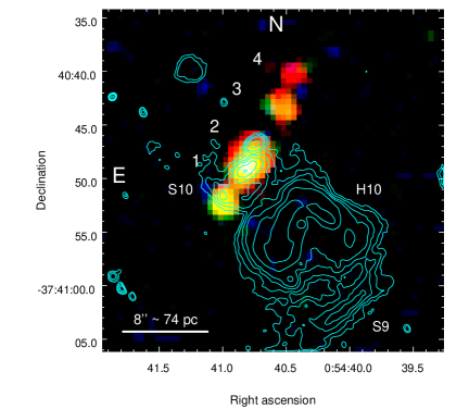
Figure 1: Stacked Chandra ACIS-I image of NGC 300 S 10, showing 4 aligned sources; we refer to those sources as “knots” 1–4, throughout this paper, as labelled in this image. Red represents 0.3–1.0 keV, green 1–2 keV, and blue 2–7 keV. The image has been adaptively smoothed with a Gaussian kernel of $\sigma=1$ pixel and has a pixel size of 0$.^{\prime\prime}$492. Cyan contours show the smoothed VLT continuum-subtracted H$\alpha$ intensity map; contour levels are arbitrary and for visualisation purposes. The complex structure of the H$\alpha$ emission can be divided into the shock-ionized S 10 region (associated with the X-ray knots), a photo-ionized H II region (H 10 in Blair & Long 1997) to the south-west of S 10, and another (smaller) shock-ionized region (the S 9 SNR in Blair & Long 1997) at the southernmost end, without an X-ray counterpart. The alignment of X-ray knots and shock-ionized optical line emission in S 10 is strongly suggestive of a jet.

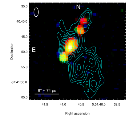
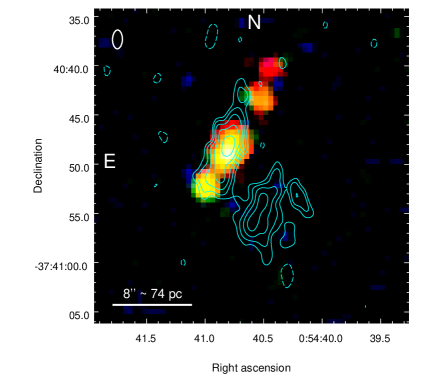
Figure 2: Top panel: Stacked Chandra ACIS-I image of NGC 300 S 10. Red represents 0.3–1.0 keV, green 1–2 keV, and blue 2–7 keV. The image has been adaptively smoothed with a Gaussian kernel of $\sigma=1$ pixel and has a pixel size of 0$.^{\prime\prime}$492. Cyan contours show the ATCA 5.5 GHz map; contour levels are $2\sigma\times\sqrt{2}^{n}$, where $\sigma=2.72\text{$\mu$}\text{Jy}$$\,{\rm beam}^{-1}$. The beam size is 2$.^{\prime\prime}$91 $\times$ 1$.^{\prime\prime}$47. Similarly to the H$\alpha$ emission (Figure 1), the radio emission consists of a component associated and aligned with the X-ray knots in the S 10 region, plus a component associated with the H 10 H II region (Blair & Long, 1997) and another component corresponding to the S 9 SNR (Blair & Long, 1997). Bottom panel: Same as top panel, but the contours are now from the ATCA 9 GHz map; contour levels are $2\sigma\times\sqrt{2}^{n}$, where $\sigma=2.78\text{$\mu$}\text{Jy}$$\,{\rm beam}^{-1}$. The beam size is 1$.^{\prime\prime}$91 $\times$ 1$.^{\prime\prime}$01. The radio emission at S 10 is spatially resolved both along the direction of the jet, and in the transverse direction, both at 5.5 GHz and at 9 GHz.

2 Data Analysis

2.1 X-ray observations

NGC 300 has been observed by Chandra a total of five times. However, in one of those observations (ID 9883) the candidate microquasar target of our study does not fall on any of the chips. A second short observation (ID 7072), taken with HRC-I, does not have the sensitivity required to detect the source. Thus, we only used three of the five observations for our X-ray data analysis (Table 1): ACIS-I observations 12238, 16028 and 16029. We downloaded the data from the public archive, and reprocessed them using standard tasks from the Chandra Interactive Analysis of Observations (ciao) Version 4.9 software package (Fruscione et al., 2006). We filtered out high particle background intervals. For our imaging analysis, we used HEASARC’s DS9 visualisation package. After we identified a number of discrete X-ray sources associated with the target of our study (as discussed in Section 3.1), we used the ciao task specextract to extract the background-subtracted spectrum for each source, in each observation. For the two southernmost sources (knots 1 and 2), we extracted the source counts from circular regions of radius $3^{\prime\prime}$; for the other two sources (knots 3 and 4), we used elliptical regions of axes $3^{\prime\prime}\times 2^{\prime\prime}$ (position angle $=330^{\circ}$), to avoid contamination from the brighter, neighbouring sources. A local background region was selected, approximately 3 times larger than the source regions. Spectral fitting was performed using XSPEC version 12.9.1 (Arnaud, 1996). Because of the low number of counts for each source, to test the goodness of our fits we used XSPEC’s implementation of W-statistics, which is Cash statistics (Cash, 1979) modified for a background-subtracted spectrum.

Table 1: Observations used for this work. The exposure time for the radio observations refers to the total time on source.

Telescope	Obs ID/Filter/$\nu$	Obs Date	Exposure
Chandra/ACIS-I	12238	2010-09-24	63.00 ks
	16028	2014-05-16	64.24 ks
	16029	2014-11-17	61.27 ks
	Total		188.51 ks
HST/ACS	F814W	2006-11-09	1542 s
	F606W	2006-11-09	1515 s
	F475W	2006-11-09	1488 s
VLT/FORS2	H$\alpha$	2010-07-10	180 s∗
	H$\alpha$/4500	2010-07-10	180 s∗
ATCA	5.5/9 GHz	2015-10-21	4.53 hr
	5.5/9.0 GHz	2015-10-22	10.75 hr
	5.5/9.0 GHz	2015-10-23	10.32 hr
	5.5/9.0 GHz	2016-08-25	9.95 hr
	5.5/9.0 GHz	2016-08-26	9.86 hr
	Total		45.41 hr

^∗ Stack of two 90 s exposures

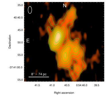
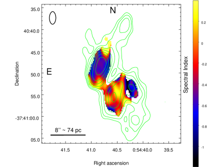
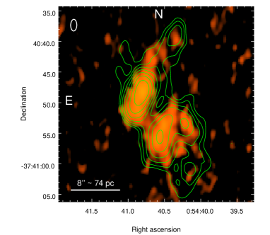
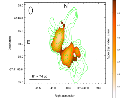
Figure 3: Top left panel: ATCA 5.5 GHz image. Contours levels are $2\sigma\times\sqrt{2}^{n}$, where $\sigma=2.72\text{$\mu$}\text{Jy}$$\,{\rm beam}^{-1}$. Bottom left panel: ATCA 9 GHz image with 5.5 GHz contours for reference. In both images, the radio nebula is aligned with the X-ray knots, which suggests that both are the result of a jet. Top right panel: Spectral index map made from the ATCA 5.5 and 9 GHz images. The 9 GHz image was convolved with the 5.5 GHz beam. We mask values below 3$\sigma$ in their respective 5.5 and 9 GHz images. Bottom right panel: Error values for our spectral index map. We find that the central source has a steep spectral index ($\alpha=-0.4\pm 0.2$), consistent with optically-thin synchrotron emission. To the southwest we see the Hii region, H 10 (Blair & Long, 1997), which, as expected, has a flatter spectral index ($\alpha\sim-0.1-0.3\pm 0.3$) than S 10.

2.2 Radio observations

NGC 300 S 10 was observed with the ATCA over three consecutive nights, starting on 2015 October 21 (proposal ID C3050). A total integration time on source of 25.6 hours was achieved. We then re-observed NGC 300 one year later, this time for two consecutive nights, 2016 August 25–26 (proposal ID C3120). For the 2015 observations, S 10 was the target and hence at the phase centre, while the follow-up observations were offset to observe another source in the same field, with the phase centre at RA $=00^{h}$55^m02$.^{s}$5, Dec $=-37^{\circ}$40^′10$.^{\prime\prime}$5, approximately 4$.^{\prime}$5 from S 10. For both observation sets, two 2048 MHz bands were observed simultaneously, centred at 5.5 GHz and 9.0 GHz, using the Compact Array Broadband Backend (CABB; Wilson et al., 2011). The telescope was in its extended 6A configuration during all of the observations, resulting in a maximum baseline of 5938.8 m. B1934$-$638 was used as both a bandpass and flux calibrator. We used B0104$-$408 as the phase calibrator. The bandpass/flux calibrator was observed at the start of the observation for 10 minutes while the phase calibrator was observed for 1 minute every 15-minute block.

We used the MIRIAD package (Sault et al., 1995) for gain and phase calibration. The data were then imaged with the Common Astronomy Software Application (CASA; McMullin et al., 2007) software package, with the CLEAN algorithm. All three nights (two nights for the 2016 observing run) of observations were stacked for each frequency and we imaged the data with Briggs weighting at a robust value of one. Finally, we combined the two observing runs to create a single mosaic image for each frequency. The cleaned, primary-beam-corrected images for both frequencies are shown in Figure 3. The 5.5 GHz image has a Gaussian restoring beam of 2$.^{\prime\prime}$91 $\times$ 1$.^{\prime\prime}$47 (position angle $-0.^{\circ}6$ East of North) and an rms noise level of $2.72\,\mu$Jy$\,{\rm beam}^{-1}$at the location of S 10. The 9 GHz image has a Gaussian restoring beam of 1$.^{\prime\prime}$91 $\times$ 1$.^{\prime\prime}$01 (position angle $-1.^{\circ}2$ East of North) and a local rms noise level of $2.78\,\mu$Jy$\,{\rm beam}^{-1}$.

In order to construct a spectral index map (Figure 3, right), we first convolved the 9 GHz image with the beam of the 5.5 GHz image. The 5.5 GHz image was then re-gridded to match the 9 GHz image, with the CASA task imregrid. We then created a two-point spectral index map (Figure 3, top right), along with a corresponding error map (Figure 3, bottom right). Both data sets were masked to their respective 3$\sigma$ thresholds prior to use.

2.3 Optical observations

2.3.1 HST imaging

We downloaded publicly available Hubble Space Telescope (HST) data for NGC 300 from the Hubble Legacy Archive. The observations (proposal ID 10915) were taken on 2006 November 9 with the Wide Field Channel (WFC) of the Advanced Camera for Surveys (ACS). We used the broadband filters F475W, F606W and F814W, with exposure times 1488 s, 1515 s and 1542 s respectively. We created a three-colour image using the F475W, F606W and F814W bands (Figure 4).

We performed aperture photometry on potential optical counterparts to the X-ray knots. Source count rates for each filter were extracted from $0.15$ arcsec (3 pixels) circular regions. We selected nearby backgrounds at least three times larger than the source regions. We used the encircled energy fractions of Sirianni et al. (2005) to determine the aperture correction and calculate the source count rates at infinite aperture. Finally, we converted count rates to physical magnitudes using the zeropoint tables for ACS-WFC.

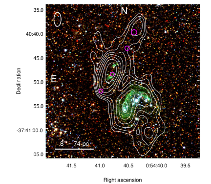
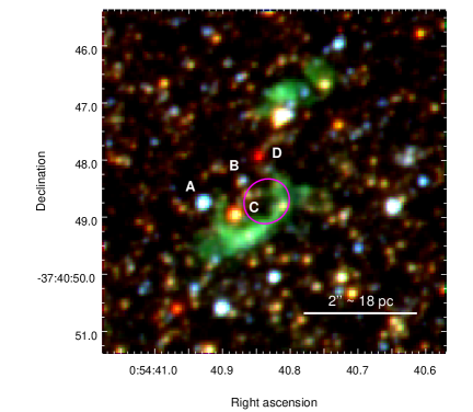
Figure 4: Top panel: HST/ACS-WFC RGB colour image of S 10. Red represents the F814W band, green is the F606W band and blue is the F475W band. Overlaid are the ATCA 5.5 GHz contours in white and, in magenta, the 95% confidence Chandra error circles (Section 2.4) for the peak-emission location of each knot. There is nebular emission (likely H$\alpha$ plus [N II], which are covered by the F606W bandpass) coincident with X-ray knot 2 and the peak radio emission. The star-forming region and photoionized nebula H 10 (Blair & Long, 1997) is to the south-west. Bottom panel: Zoomed-in image of the inner part of the S 10 complex around the extended X-ray knot 2, more clearly showing the two separate nebulae (in green). The magenta circle represents the 95% confidence Chandra central position of the brightest knot (Section 3.3.2). Letters indicate potential optical counterparts for the accreting compact object, origin of the jet. The distinct morphology of the line-emitting nebula around the peak X-ray and radio emission could be a result of anisotropic ejecta from a progenitor SN or it could be gas shock-ionized by the jet and the counterjet.

2.3.2 VLT imaging

Finally, from the ESO Science Archive Facility, we downloaded publicly available Very Large Telescope (VLT) data to better study the narrow-band H$\alpha$ emission. NGC 300 S 10 was observed on 2010 July 10 with two consecutive FORS2 90 s exposures (with the first exposure starting at Universal Time 09:54:45) with the “H_Alpha+83” interference filter. The filter has a central wavelength of 6563 Å and a full width at half maximum (FWHM) of 61 Å; thus, it also includes the [N ii]$\lambda\lambda$6548,6583 lines. The collimator was in standard resolution. The seeing was $\approx$0$.^{\prime\prime}$6 and the airmass 1.03. This was followed by two consecutive 90 s exposures with the “H_Alpha/4500+61” interference filter, centred at 6665 Å, for continuum subtraction.

We stacked the two 90 s H$\alpha$ exposures and the corresponding continuum exposures using the Image Reduction and Analysis (iraf) software Version 2.16 (Tody, 1993) package imcombine. We aligned the stacked H$\alpha$ and continuum images with the iraf package ccmap, relying on $\approx 30$ common bright sources. Finally, we subtracted the continuum using the iraf package imarith. The resulting image is displayed in Figure 5. We used the continuum-subtracted image for flux measurements (Section 3.3).

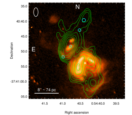
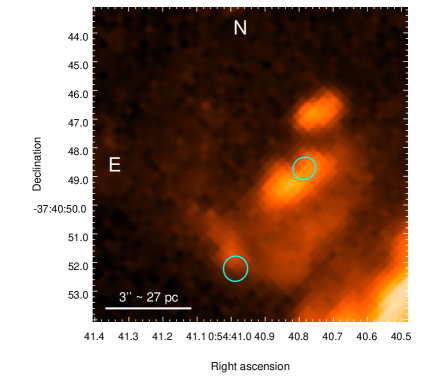
Figure 5: Top panel: smoothed VLT/FORS2 continuum-subtracted H$\alpha$ image of S 10 with the Chandra 95% error circles for the four X-ray knots in cyan and 5.5 GHz ATCA contours overlaid in green. As already noted in the HST image (Figure 4), the two regions with the strongest H$\alpha$ emission are located on either side of X-ray knot 2. However, the VLT image also shows a larger H$\alpha$ nebula, extending south as far as X-ray knot 1. Bottom: Zoomed-in view of the core region, from the continuum-subtracted VLT/FORS2 image. The cyan circles mark the position of X-ray knots 1 and 2.

2.4 Astrometric alignment

The default Chandra/ACIS-I astrometry is known to be accurate within $\approx$0$.^{\prime\prime}$75 for 90% of the observations. To improve on this value, we aligned the stacked Chandra image to the DR1 Gaia astrometric frame (Lindegren et al., 2016; Gaia Collaboration et al., 2016b, a), which has a mean uncertainty $\sigma\approx 0.3$ mas. Because of the low number of X-ray sources, we were only able to find five common, bright point sources suitable for frame alignment. After alignment, we find position error residuals of $\approx$0$.^{\prime\prime}$1–0$.^{\prime\prime}$2. We determined the central position of each X-ray source using the ciao task wavdetect on the stacked Chandra/ACIS-I image. To estimate their respective confidence error circles, we calculated the 95% statistical uncertainty for the central position of each source using Eq. (5) from Hong et al. (2005); we then combined (in quadrature) those statistical uncertainties and the Chandra/Gaia alignment residuals. We also aligned our HST images in the F475W, F606W and F814W bands and our VLT H$\alpha$/4500 and H$\alpha$ bands onto the Gaia astrometric frame, using $>100$ common, bright, non-saturated sources. This provides a positional accuracy within 0$.^{\prime\prime}$009 for the HST images and 0$.^{\prime\prime}$03 for the VLT images. We assume that the radio and Gaia astrometric frames are consistent with each other, within the relative uncertainties.

Table 2: Central position of each X-ray knot; knot 2 is spatially resolved, while knots 1, 3 and 4 are unresolved.

	RA (J2000)	Dec (J2000)
Knot 1	00h54m40$.^{s}$99 $(\pm 0.^{\prime\prime}44)$	$-37^{\circ}$40′52$.^{\prime\prime}$2 $(\pm 0.^{\prime\prime}42)$
Knot 2	00h54m40$.^{s}$79 $(\pm 0.^{\prime\prime}41)$	$-37^{\circ}$40′48$.^{\prime\prime}$7 $(\pm 0.^{\prime\prime}38)$
Knot 3	00h54m40$.^{s}$53 $(\pm 0.^{\prime\prime}48)$	$-37^{\circ}$40′43$.^{\prime\prime}$3 $(\pm 0.^{\prime\prime}45)$
Knot 4	00h54m40$.^{s}$41 $(\pm 0.^{\prime\prime}57)$	$-37^{\circ}$40′40$.^{\prime\prime}$0 $(\pm 0.^{\prime\prime}55)$

3 Results

3.1 X-ray results

3.1.1 X-ray knots

The Chandra data reveal the presence of four X-ray sources that appear linearly aligned with a total projected length of $\approx 17^{\prime\prime}\approx 150\,\text{pc}$ (Figure 2). No other X-ray sources are detected within a circle of radius $\approx 1^{\prime}$. Additionally, we only expect $\approx 4\times 10^{-3}$ extragalactic sources (Lehmer et al., 2012) with $0.5-2.0\,\text{keV}$ fluxes greater than $f_{0.5-2.0\,\text{keV}}=1.9\times 10^{-15}\,\text{erg cm${}^{-2}$ s${}^{-1}$}$ (the flux of the dimmest source, knot 4) within a region equivalent to the projected area of the radio bubble (i.e.,  $19^{\prime\prime}\times 6^{\prime\prime}\approx 8.80\times 10^{-6}$ deg²); therefore a physical connection between those aligned sources is highly likely. We shall refer to those four visually distinct X-ray sources as knots 1 to 4 (starting from the southernmost one). The central positions of those four knots are listed in Table 2.

Of those four sources, knot 2 appears, at first sight, spatially extended (Figure 2) and larger than the other three. We quantified this visual impression with the MARX simulation software. Using the task simulate_psf, we simulated 1000 point-spread functions (PSFs) at the location of S 10 on the ACIS-I chip during ObsID 16028. For this ensemble of simulated PSFs, the average encircled energy fraction as a function of radius was determined with the ciao task ecf_calc. We compared this value to the observed encircled energy fraction of knot 2 during ObsID 16028. The results are displayed in Figure 6. The shape of the PSF does not match that observed for knot 2 and proves that knot 2 is indeed extended. It is consistent with two point-like sources separated by $\approx$1$.^{\prime\prime}$2 and oriented roughly along the same direction defined by the other knots.

There are insufficient counts to do meaningful spectral analysis on the individual X-ray knots for individual epochs. However, we can investigate source variability and evolution of the hardness ratios from the three epochs spaced over $\approx$4 years. For the hardness ratios, we defined the soft band as $0.3$–$1.2\,\text{keV}$ (by analogy with the combined ultra-soft and soft bands in the Chandra Source Catalogue; Evans et al. 2010), and $1.2$–$7.0\,\text{keV}$ for the hard band. Since the ACIS-I detector has lost sensitivity over the years, especially in the soft band, we must correct the count rates measured in ObsID 12338 (Cycle 11) to make them comparable with the count rates measured in Cycle 15 (ObsIDs 16028 and 16029). We did that using the online tool pimms version 4.8e. For knot 1, we assumed a thermal plasma model with temperature $kT\approx 0.8\,\text{keV}$, while for knots 2, 3 and 4 we assumed a temperature of $kT\approx 0.4\,\text{keV}$. These assumptions are based on our spectral fitting after we combined the spectra from all three Chandra epochs, as described later in this section. The cycle-corrected hard and soft count rates are displayed in Table 3. We find no significant variability for any of the knots, in either band, over all three epochs. The corresponding hardness ratios are displayed in Table 4. While knots 2, 3 and 4 all have similar spectral hardnesses, knot 1 appears harder. As with the count rates, no significant variability is detected across all four knots and all three epochs.

In order to conduct spectral modelling of the knots, we stacked the three Chandra epochs. Each of the knots has insufficient counts for $\chi^{2}$ statistics and so w-statistics were used. We first attempted to fit each of the knots with a simple absorbed power-law model (TBabs $\times$ po). However all power-law fits yielded unphysically high absorption and photon indices. For example, fitting knot 2 with an absorbed power-law model yields a best-fit photon index $\Gamma\approx 10$ and column density $n_{\rm H}=10^{22}\,\text{c}\text{m}^{-2}$, for a w-statistic of 87.7 and 72 degrees of freedom. Instead, we find (Table 5) that all four knots are well described by thermal plasma models, such as mekal (Mewe et al., 1985; Mewe et al., 1986) (Figure 7). No additional intrinsic absorption is required, and thus we use a single TBabs component fixed to the line-of-sight column density towards NGC 300 ($N_{\rm H}=3\times 10^{20}\,\text{c}\text{m}^{-2}$; Dickey & Lockman 1990; Kalberla et al. 2005). As expected from the hardness ratios (Table 4), knot 1 appears hotter than the rest. The unabsorbed X-ray luminosities of the knots ranges from $\approx$1 $\times 10^{36}\,\text{erg s${}^{-1}$}$ for the dimmest knot (knot 4) to $\approx$7 $\times 10^{36}\,\text{erg s${}^{-1}$}$ for the brightest (knot 2). For the spectrum of the combined emission of all knots, we find a best-fitting thermal plasma temperature $T\approx 0.6\,\text{keV}$ and an unabsorbed bolometric luminosity $L\approx 1.1\times 10^{37}\,\text{erg s${}^{-1}$}$. The model for this best-fitting thermal plasma is shown in Figure 7 with the fit parameters displayed in Table 5. While the spectrum is well fitted by thermal plasma alone, we also try a thermal plasma plus power-law model. We fix the power-law photon index to $\Gamma=1.7$, typical of X-ray binaries with X-ray luminosities similar to the core of S 10 (see Sections 3.1.2 and 4.4 for more details). However, we find no statistically significant improvement to the fit, with a maximum power-law contribution of $L<2\times 10^{36}\,\text{erg s${}^{-1}$}$ at the 90% confidence level. Thus, by Occam’s razor, our preferred model is the simple best-fitting thermal plasma model.

The normalisation constant for the mekal component (at zero redshift) is defined as $K=10^{-14}\,\int(n_{e}\,n_{\rm H}\,dV)/(4\pi d^{2})\approx 10^{-14}\,n_{e}^{2}\,V/(4\pi d^{2})$, where $V$ is the volume of the emitting region, $n_{e}$ is the electron density, $n_{\rm H}$ is the nuclear density and $d$ is the distance. We approximate the X-ray structure as five spherical sources (two of them corresponding to knot 2) with radii similar to or smaller than the Chandra resolution, $\approx$0$.^{\prime\prime}$4 $\approx 1.1\times 10^{19}\,\text{c}\text{m}$; this corresponds to a total volume $V\lesssim 3\times 10^{58}\,\text{c}\text{m}^{3}$ for the emitting plasma region. Thus, for the best-fitting normalisation $K\approx 9\times 10^{-6}$ in our spectral model (Table 5), we estimate a lower limit to the density of the hot plasma component, $n_{e}\gtrsim 4\,\text{c}\text{m}^{-3}$.

Table 3: Chandra/ACIS-I count rates for the hard (1.2–7.0 keV) and soft (0.3–1.2 keV) bands. Chandra Obs 12238 (Cycle 11) has been scaled to match the Chandra sensitivity of the other observations (Cycle 15). Count rates are in units of $10^{-4}$ count s^-1.

Obs ID	Knot 1		Knot 2		Knot 3		Knot 4		Combined
	Hard	Soft	Hard	Soft	Hard	Soft	Hard	Soft	Hard	Soft
12238	$1.8\pm 0.6$	$2.3\pm 0.6$	$2.7\pm 0.7$	$9.5\pm 1.1$	$\leq 0.4$	$2.4\pm 0.5$	$0.4\pm 0.3$	$0.7\pm 0.3$	$5.0\pm 1.0$	$15.6\pm 1.4$
16028	$2.4\pm 0.6$	$1.9\pm 0.5$	$2.5\pm 0.7$	$10.9\pm 1.3$	$0.5\pm 0.4$	$2.3\pm 0.6$	$\leq 0.6$	$1.4\pm 0.5$	$6.0\pm 1.0$	$17.0\pm 1.6$
16029	$1.5\pm 0.5$	$3.9\pm 0.8$	$1.9\pm 0.6$	$7.0\pm 1.1$	$0.7\pm 0.4$	$1.3\pm 0.5$	$0.4\pm 0.1$	$0.3\pm 0.2$	$4.6\pm 0.9$	$12.9\pm 1.5$
Total	$2.1\pm 0.3$	$3.0\pm 0.4$	$2.4\pm 0.4$	$10.2\pm 0.7$	$0.5\pm 0.2$	$2.4\pm 0.4$	$0.3\pm 0.2$	$0.9\pm 0.2$	$5.2\pm 0.6$	$16.7\pm 0.9$

Table 4: Hardness ratios corresponding to the count rates listed in Table 3. The hardness ratios are defined as (1.2–7.0 keV)/(0.3–1.2 keV).

Obs ID	Knot 1	Knot 2	Knot 3	Knot 4	Combined
12238	$0.78\pm 0.33$	$0.28\pm 0.08$	$\leq 0.17$	$0.57\pm 0.49$	$0.32\pm 0.07$
16028	$1.27\pm 0.50$	$0.23\pm 0.07$	$0.22\pm 0.16$	$\leq 0.41$	$0.35\pm 0.07$
16029	$0.38\pm 0.16$	$0.27\pm 0.09$	$0.50\pm 0.33$	$1.1\pm 0.8$	$0.36\pm 0.08$
Total	$0.70\pm 0.15$	$0.23\pm 0.04$	$0.19\pm 0.08$	$0.28\pm 0.18$	$0.31\pm 0.04$

3.1.2 X-ray core

If, as we suggest, S 10 is a powerful microquasar within NGC 300, then we expect to find a hard X-ray source at its core, a signature of accretion. However, we do not observe this; all the knots are best-fitted with soft thermal plasma models, with the majority of emission being $<2\,\text{keV}$. We do find a marginal detection of $6^{+8}_{-5}$ net counts in the 2–7 keV band, near the central position of the brightest knot (knot 2). However, this is also consistent with the $\approx$5.8 net counts expected from a thermal plasma at a temperature of $0.53\,\text{keV}$, fitted to the spectrum of knot 2. From that, we estimate a 90% upper limit of $\approx$6 $\times 10^{-5}$ net ct s^-1 from a point-like power-law core (in addition to the soft thermal emission). For an assumed photon index $\Gamma=1.7$, this corresponds to a luminosity $L_{0.3-8}\approx 10^{36}$ erg s^-1. No other knots have significant 2–7 keV emission, and thus, regardless of where the central source is, we can take this value as the upper limit of the current accretion luminosity of the central engine.

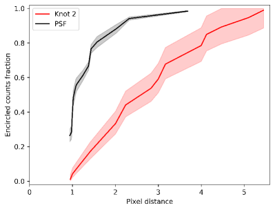
Figure 6: Enclosed ACIS-I count fraction as a function of distance from the centre of a source. The black points represent the PSF of Chandra/ACIS-I, from a 1000-iteration Monte Carlo simulation, at the location of S 10, for ObsID 16028. The red points represent the measured extent of knot 2 from the same observation. Shaded regions indicate 1-sigma errors. At the distance of 1.88 Mpc, 1 ACIS-I pixel corresponds to $\approx$4.5 pc. The comparison shows that the source is significantly extended.

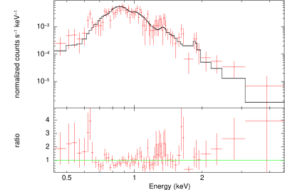
Figure 7: Chandra/ACIS-I stacked spectrum of the combined knots emission from observations 12238, 16028 and 16029, fitted with a thermal plasma model; the best-fitting plasma temperature is $kT=(0.6\pm 0.1)\,\text{keV}$. See Table 5 for the fit parameters.

In the absence of a well-resolved, point-like hard source, we can use indirect arguments to constrain the possible location of the candidate microquasar core. Spatially resolved X-ray jets comprising a series of bright knots are seen in some AGN: most famously, in M 87 (Wilson & Yang, 2002; Marshall et al., 2002a) and NGC 5128 (Kraft et al., 2002; Hardcastle et al., 2003). In those cases, the active nucleus is generally located at one end of the string of X-ray knots, because the jet coming towards us is much brighter than the (usually undetected) counter-jet. In the NGC 300 candidate microquasar, this would correspond to knot 1 (which is also the one with the hardest X-ray colours and hottest mekal fit temperatures). However, the lobe-like morphology of the inner knot of H$\alpha$ emission (pointing towards the south-east: Figure 4), and the shape of the larger H$\alpha$ bubble (Figure 5) suggest that knot 1 is unlikely to be the origin of the jet, and that the core is most likely associated with knot 2 (the most luminous part of the system in X-rays, radio and H$\alpha$). We have already shown that knot 2 is extended (Figure 6), and suggest that it likely consists of two sources separated by $\approx$1.2$\arcsec$ and also aligned in the general direction of the other knots. Thus, we suggest that knot 2 consists of a pair of ejecta or hot spots from the approaching and receding jet and that the core resides somewhere between the two.

Table 5: Best-fitting parameters for the spectra of the individual knots and for the combined spectrum, from the merged Chandra/ACIS-I observations 12238, 16028 and 16029, fitted with TBabs $\times$ mekal. We fixed the absorbing column density $N_{\rm H}$ to the Galactic line-of-sight value; adding intrinsic local absorption does not produce statistically significant improvements. Errors are 90% confidence limits for one interesting parameter. We report the observed fluxes and de-absorbed luminosities.

Model	Parameter	Knot 1	Knot 2	Knot 3	Knot 4	Combined
	Net Counts (0.3–7.0 keV)	99	234	58	26	432
TBabs	$N_{\rm H}\Big{(}10^{22}\,\text{c}\text{m}^{-2}\Big{)}$	[0.03]	[0.03]	[0.03]	[0.03]	[0.03]
Mekal	$k_{e}T$ (keV)	$0.80_{-0.14}^{+0.15}$	$0.53_{-0.10}^{+0.07}$	$0.37_{-0.08}^{+0.15}$	$0.28_{-0.07}^{+0.31}$	$0.57_{-0.06}^{+0.05}$
	K $\Big{(}10^{-6}\Big{)}$	$2.1_{-0.3}^{+0.4}$	$5.8_{-0.8}^{+1.3}$	$1.8_{-0.6}^{+0.9}$	$1.2_{-0.7}^{+1.3}$	$9.2_{-0.9}^{+1.0}$
	$f_{0.3-8.0}$ $\Big{(}10^{-15}\text{erg cm${}^{-2}$ s${}^{-1}$}\Big{)}$	$4.7_{-0.8}^{+0.8}$	$14.4_{-1.9}^{+1.9}$	$3.8_{-1.1}^{+1.1}$	$2.1_{-1.3}^{+1.3}$	$22.9_{-2.2}^{+2.2}$
	$L_{0.3-8.0}$ $\Big{(}10^{36}\,\text{erg s${}^{-1}$}\Big{)}$	$2.2_{-0.4}^{+0.4}$	$6.9_{-0.9}^{+0.9}$	$1.9_{-0.6}^{+0.6}$	$1.1_{-0.7}^{+0.7}$	$11.0_{-1.1}^{+1.0}$
	w-statistic/d.o.f.	79.3/55	64.2/73	37.6/37	14.1/15	115.8/108

3.2 Radio results

From the ATCA images, we discovered a bright, resolved and elongated radio structure aligned along the axis of the X-ray knots (Figure 2). The majority of the radio emission comes from a region coincident with the first and second X-ray knots, with the radio peak coincident with X-ray knot 2. In the 5.5 GHz image, we also detect a region of enhanced radio emission, which we refer to as a ‘radio node’, north-west of the bright, central radio component, near X-ray knot 4; the same radio node is a marginal detection at 9 GHz. From the 5.5 GHz image, we measure a total size of the elongated radio bubble as $19^{\prime\prime}\times 6^{\prime\prime}\approx 170\times 55\,\text{pc}$ (for a distance of 1.88 Mpc). This emitting region is clearly resolved both along and across the jet direction, because the beam size is only $\approx$26 $\times$ 13 pc (Section 2.2).

We find total integrated flux densities of $f_{5.5\,\text{GHz}}=520\pm 15\,\text{$\mu$}\text{Jy}$ and $f_{9\,\text{GHz}}=380\pm 20\,\text{$\mu$}\text{Jy}$ for the 5.5 and 9 GHz bands, respectively. This equates to a 5.5 GHz radio luminosity of $L_{\rm 5.5\,\text{GHz}}\approx 1.2\times 10^{34}\,\text{erg s${}^{-1}$}$. We fitted a 2-dimensional Gaussian profile to the central, and brightest, region of S 10 using the CASA task imfit, to estimate the flux density coming from the core. We find peak intensities of $87.8\pm 2.7\,\text{$\mu$}\text{Jy}$$\,{\rm beam}^{-1}$and $35.0\pm 2.8\,\text{$\mu$}\text{Jy}$$\,{\rm beam}^{-1}$at 5.5 and $9\,\text{GHz}$ respectively, and integrated flux densities of $429\pm 30\,\text{$\mu$}\text{Jy}$ and $371\pm 29\,\text{$\mu$}\text{Jy}$. We also used a 2-dimensional Gaussian profile fit in the 5.5 GHz map to measure the integrated flux of the radio node to the northwest of the core; we find a flux density of $79.5\pm 5.3\,\text{$\mu$}\text{Jy}$. The knot is only marginally detected in the 9 GHz image, with an integrated flux density of $17.9\pm 4.4\text{$\mu$}\text{Jy}$. Our measured radio fluxes are summarised in Table 6.

The spectral index $\alpha$ (defined as $f_{\nu}\propto\nu^{\alpha}$) ranges from about $-0.7$ to about $-0.4$ near the central region (where the radio emission is strongest), at the location of X-ray knot 2 (Figure 3). This is consistent with optically-thin synchrotron emission. There are also hints of a flattening of the spectral index towards the edges (near X-ray knots 1 and 3). We also measured the spectral index of the radio node at the north-west end of the bubble, finding $\alpha=-1.3\pm 0.9$ there. It is unclear whether this radio node is associated with the X-ray knot 4, as the peak radio emission (in the 5.5 GHz band) of the radio node appears to be slightly offset to the north-west of the X-ray knot (Figure 2, top panel).

We also detect radio emission from the nearby, possibly unassociated Hii region H 10 (Blair & Long, 1997), south-west of S 10 (Figure 3). The spectral index in this region is much flatter than in the candidate microquasar bubble (Figure 3), as expected for the spectral index of an Hii region. At $5.5\,\text{GHz}$, the peak flux density of the Hii region is $(52.6\pm 2.7)\,\text{$\mu$}\text{Jy}$$\,{\rm beam}^{-1}$and the integrated flux density is $(511\pm 15)\,\text{$\mu$}\text{Jy}$. At $9\,\text{GHz}$, the peak flux density is $(30.1\pm 2.8)\,\text{$\mu$}\text{Jy}$$\,{\rm beam}^{-1}$and the integrated flux density is $(302\pm 24)\,\text{$\mu$}\text{Jy}$. A few arcsec further to the south-west, another region with steep spectral index corresponds to the supernova remnant catalogued as S 9 in Blair & Long (1997). A study of H 10 and S 9 is beyond the scope of this work.

3.3 Optical results

3.3.1 Diffuse emission

Blair & Long (1997) used CCD imaging and spectroscopic data taken in 1987 with the 2.5-m du Pont telescope to measure H$\alpha$ and [S ii] fluxes of optical SNR candidates in NGC 300. Their source S 10 = DDB2 corresponds to the X-ray and radio structures discussed in this paper. S 10 is listed in the catalogue of Blair & Long (1997) with a line ratio [S ii]:(H$\alpha$ plus [N ii]) $\approx 0.67$, indicative of shock-ionized gas, and with an H$\alpha$ flux $F_{\rm H\alpha}\approx 8.3\times 10^{-15}\,\text{erg cm${}^{-2}$ s${}^{-1}$}$ (Blair & Long, 1997, from the average surface brightness and size, in their Table 3A). This value has already been corrected for spectral contamination from [N ii]$\lambda\lambda$6548,6583, which Blair & Long (1997) assumed to be 25% of the H$\alpha$ emission, based on an average value over their sample of SNR candidates in NGC 300. In fact, individual long-slit spectra of S 10 also from Blair & Long (1997) show a slightly larger [N ii] contribution of $\sim$35%, implying an H$\alpha$ flux $F_{\rm H\alpha}\approx 7.7\times 10^{-15}\,\text{erg s${}^{-1}$}$. The diameter of this line-emitting region was reported by Blair & Long (1997) as only $\approx$14 pc. This is much smaller than the size of the H$\alpha$ structure we see for example in the VLT images (Figure 5). We suspect that the S 10 measurements of Blair & Long (1997) refer only to the brightest core of the nebula, near X-ray knot 2, not to the larger structure around it. Thus, we expect the total H$\alpha$ flux from the whole region to be a few times larger.

In 2006, follow-up spectroscopic observations of NGC 300 by Millar et al. (2011), with the 2.3-m Advanced Technology Telescope at Siding Spring Observatory, indicated a slightly lower [Sii]:H$\alpha$ ratio of $0.35\pm 0.15$ for S 10, although the source was still classified as an SNR based on its multiband properties. More importantly, Millar et al. (2011) found that the S 10 emission region is significantly larger (diameter of $\approx$56 pc) than originally reported, and an order of magnitude more luminous ($F_{\rm H\alpha}=(10.5\pm 1.4)\times 10^{-14}\,\text{erg cm${}^{-2}$ s${}^{-1}$}$). This flux value was based on the extrapolation to the whole nebula of the integrated line flux measured from a long-slit observation; such extrapolations are fraught with uncertainties. Moreover, at the average seeing of Siding Spring Observatory, S 10 is inevitably contaminated by emission from the nearby H 10 Hii region, which may explain the lower value of [Sii]:H$\alpha$ measured by Millar et al. (2011). Size and flux discrepancies for several other NGC 300 sources between Blair & Long (1997) and Millar et al. (2011) are also discussed in the latter paper.

To improve on those previous two studies and resolve their discrepancies, we investigated the diffuse optical emission at S 10 using archival HST/ACS images in the F475W, F606W and F814W filters (Figure 4). This is possible because the broadband filter F606W also includes the wavelengths around H$\alpha$; therefore, we expect regions of strong H$\alpha$ emission to show up in green, in a true-colour image from those three bands. There are indeed two bright regions of H$\alpha$ emission (Figure 4, bottom panel), separated by a distance of $\approx$20 pc, on either side of the central location of X-ray knot 2. The southern H$\alpha$ source has a lobe-like structure, which suggests that the gas has been shocked by some kind of fast ejection: either a microquasar jet or collimated ejecta during a SN explosion. The lobe-like source has a diameter of $\approx$0$.^{\prime\prime}$8, corresponding to $\approx$15 pc; it is aligned along the same direction defined by the string of X-ray knots and by the elongated radio source. This is most likely the source identified and measured by Blair & Long (1997, their Fig. 3).

To investigate the presence of fainter, much more extended H$\alpha$ emission, and to measure its flux, we used the continuum-subtracted VLT image. Although at lower spatial resolution, we clearly recover (Figure 5) the two innermost H$\alpha$ emission regions already seen in the broadband HST image. Additionally, we see an extended bubble, stretching between and around X-ray knots 1 and 2 (characteristic size of $\approx$60 pc), with a brighter spot almost coincident with X-ray knot 1 (Figure 5). The emission region is bounded on its southern side by a slightly brighter rim. We speculate that this H$\alpha$-emitting bubble has been inflated by a source of kinetic power probably located near X-ray knot 2: the same source of kinetic power responsible for the radio and X-ray emission.

To measure the flux of the extended H$\alpha$ region, we defined suitable source and background regions in the continuum-subtracted VLT image (Figure 5), with the imaging and photometry tool DS9. We then used the VLT FORS2 Exposure Time Calculator in Imaging Mode to convert from the measured net count rate to a physical line emission flux. We assumed a contribution of [N ii]$\lambda\lambda$6548,6583 equal to $(30\pm 5)$% of the H$\alpha$ flux. This choice is based on the line ratios measured directly for S 10 by Blair & Long (1997) and Millar et al. (2011), and takes also into account the small fraction of [N ii] flux that falls outside the VLT filter passband. We obtain a flux $F_{\rm H\alpha}=(4.1\pm 0.5)\times 10^{-14}\,\text{erg cm${}^{-2}$ s${}^{-1}$}$. The error is the quadrature sum of the uncertainty on the [N ii]$\lambda\lambda$6548,6583 contribution and a rough estimate of the range of values we obtained for slightly different choices of the outer boundary of the S 10 bubble. We also verified this flux estimate by estimating the ratio (a factor of 5) between the H$\alpha$ counts in the whole bubble and in the bright core, for which Blair & Long (1997) had reported a flux of $\approx$8$\times 10^{-15}\,\text{erg cm${}^{-2}$ s${}^{-1}$}$. Finally, we confirmed the consistency of our estimate by comparing our measured VLT count rates for S 10 and for isolated SNR candidates that have a more reliable flux measurement in Blair & Long (1997); we obtained the same estimate of an S 10 H$\alpha$ flux between $\approx$4–5$\times 10^{-14}\,\text{erg cm${}^{-2}$ s${}^{-1}$}$. At the distance of 1.88 Mpc, this corresponds to a luminosity $L_{H\alpha}=(1.7\pm 0.2)\times 10^{37}\,\text{erg s${}^{-1}$}$ and (for a standard Balmer decrement from Case B recombination) $L_{H\beta}=(6\pm 1)\times 10^{36}\,\text{erg s${}^{-1}$}$.

Table 6: Integrated ATCA 5.5 amd 9 GHz fluxes. For fluxes values obtained via the CASA task imfit we provide spectral indices. The steep spectral index of the core suggests that the emission is coming from optically-thin synchrotron emission, as expected from other radio bubbles.

Object	5GHz flux	9GHz flux	$\alpha$
	$\mu$Jy	$\mu$Jy
Total	$520\pm 15$	$380\pm 20$
Core	$429\pm 30$	$352\pm 29$	$-0.4\pm 0.2$
Node	$75\pm 7$	$39\pm 17^{*}$	$-1.3\pm 0.9$
H ii Region	$511\pm 15$	$302\pm 24$

^∗ Flux integrated over region defined by radio node in $5.5\,\text{GHz}$ image

3.3.2 Stellar counterparts

We selected a few potential optical counterparts in the HST images (Figure 4) located close to knot 2, as this is the most likely location of the true nuclear source (as discussed in Section 3.1.2 and from the H$\alpha$ morphology discussed in Section 3.3.1); we measured their optical brightnesses and colours with iraf. We interpreted their physical properties by comparing those values with the Padova theoretical stellar isochrones (Bressan et al., 2012; Chen et al., 2015) for a metallicity $Z=0.015$ (Table 7). Specifically, we estimated the age, mass, radius and temperature on the nearest isochrone to each star. In doing so, we assumed that any emission we see is due to a single star and not to an accretion disc around the compact object or to multiple stars. Star A is the bluest and brightest stellar source in the field, a B-type giant; however, it appears unlikely to be the true optical counterpart of the central engine, as it resides outside of a lobe-shaped H$\alpha$ nebula (Figure 4), and therefore, offset from the likely direction of the jet that inflated that structure. Star C is also outstanding in brightness and colour from the rest of the stellar population in the field: it is consistent with an intermediate-age AGB star (near the top of the AGB branch), and it lies along the direction of the jet. Perhaps the most intriguing candidate optical counterpart is star D. It is also located along the direction of the jet, approximately half way between the two peaks of H$\alpha$ emission (Figure 4). It is detected as a moderately bright source only in the F814W image (Vegamag $m_{814}\approx 23.1$ mag). Its extremely red colour ($m_{606}-m_{814}>2.6$ mag;$m_{475}-m_{814}>3.2$ mag) suggest a high intrinsic reddening, higher than for any other neighbouring star; this could be due for example to circumstellar dust. For example, among the possible alternative interpretations, we cannot rule out that star D is a hypergiant or Wolf-Rayet star with intrinsic absolute brightness $M_{V}<-7$ mag, but a strong extinction $A_{V}\gtrsim 7$ mag. We shall mention later (Section 4.2) that a massive donor star surrounded by shells of ejected material is consistent with one of the scenarios discussed for the feeding of this candidate microquasar. Further investigations on the nature of star D is beyond the scope of this paper. A discussion on the relative contributions of accretion disk and donor star to the optical emission is also left to further work.

We also searched for unusually bright, point-like optical sources at the location of the other X-ray knots, but did not find any unusual candidate. Most of the other stars visible in the HST image of the field (Figure 4) are red giants from an intermediate-age population (age of $\sim$ a few $10^{8}$ yr), with a few B-type main sequence stars from a younger population.

Table 7: HST magnitudes and physical parameters of four potential optical counterparts of the true nuclear source of S 10. The optical counterparts (along with the lettering) corresponds to those outlined in Figure 4. Observed magnitudes are converted to physical properties using the theoretical isochrones for a metallicity $Z=0.015$. The stellar radii are calculated using the surface gravity and total mass. Colours for star D are dominated by intrinsic reddening and thus comparison to theoretical isochrones is meaningless.

Star	F814W	F606W	F475W	Age	Mass	Radius	Temperature	Luminosity
	mag	mag	mag	Myr	${\rm M}_{\odot}$	${\rm R}_{\odot}$	K	erg s-1
A	$-3.67\pm 0.02$	$-3.86\pm 0.02$	$-3.88\pm 0.02$	$\sim 50$	7	110	12,300	$2\times 10^{37}$
B	$-2.77\pm 0.07$	$-2.10\pm 0.05$	$-1.86\pm 0.06$	$\sim 200$	4	120	6,600	$2\times 10^{36}$
C	$-4.91\pm 0.01$	$-2.30\pm 0.06$	$-0.66\pm 0.05$	$\sim 500$	3	1,600	3,400	$2\times 10^{37}$
D	$-3.30\pm 0.04$	$\geq-0.7$	$\geq-0.1$	N/A	N/A	N/A	N/A	N/A

As in our ATCA data, the Hii region to the south-west, H 10 (Blair & Long, 1997), is clearly visible. The HST images show that there is strong F606W emission coincident with a population of bright, blue stars (Figure 4).

4 Discussion

We have identified a chain of four thermal X-ray sources aligned with each other and with an elongated 170-pc-long radio structure. The X-ray and optical sources are associated with an optical nebula originally identified as an SNR, but which is also reminiscent of jet-powered ULX bubbles. Here, we argue that the most likely explanation for the multiband structure is that S 10 is a powerful microquasar, although we also consider alternative explanations. The X-ray spectra for the knots are dominated by optically-thin thermal plasma emission, likely a result of jet/ISM interactions. The radio emission has a steep spectral index, consistent with optically-thin synchrotron emission; this is consistent with a relativistic electron population energized by a microquasar jet. Finally, the associated optical line-emission regions are shock-ionised, consistent with a forward shock propagating into the ISM, caused by the impact of a microquasar jet or fast SN ejecta. This is displayed in Figure 8, where the Chandra, ATCA and VLT images have been aligned and rotated to demonstrate the connections between structures observed in each band. In this section, we collate and examine in more detail the observational properties of S 10 that have led to our microquasar interpretation. Finally, we attempt to determine the jet power of S 10.

4.1 Emission processes in the knots

An important finding of our Chandra analysis is that the X-ray emission is from thermal plasma. This is likely the result of jet-driven shocks propagating into the ISM. The density inferred for the X-ray emitting hot plasma (Section 3.1) is consistent with typical pre-shock ISM densities $\sim$ 1 cm^-3. It is hard to compare the knotty structure of the NGC 300 candidate microquasar (Figure 8) with the fine details of X-ray jet knots seen in nearby AGN such as M 87 and NGC 5128, because of the much higher spatial resolution (relative to jet length) and signal-to-noise ratio for the latter class of jets. Instead, the Chandra images of the S 10 jet are reminiscent of the X-ray appearance of jets in higher-redshift radio galaxies and quasars (e.g.,  Massaro et al., 2011, 2015; McKeough et al., 2016). However, appearances can be deceptive. The X-ray emission from AGN and quasar jets (including the emission from their hot spots) is almost always non-thermal (Harris & Krawczynski, 2006): either synchrotron radiation from relativistic electrons (with Lorentz factors $\gamma\gtrsim 10^{7}$), or inverse Compton scattering of cosmic microwave background photons off slightly less energetic electrons ($\gamma\sim 10^{3}$). The only few exceptions, where X-ray hot spots have been attributed to thermal emission, are sources in which the AGN jet is colliding with a dense, cold cloud; e.g., the jets in the radio galaxies PKS 2152$-$699 (Ly et al., 2005), 4C$+$29.30 (Siemiginowska et al., 2012), and 3C 277.3 (Worrall et al., 2016). Instead, in both of the known off-nuclear microquasars (NGC 7793 S 26 and NGC 300 S 10) with evidence of X-ray jets, the hot spots are dominated by thermal emission at temperatures $\sim$0.5 keV. In both sources, the total X-ray emission from shocked gas is $\sim 2\times 10^{37}\,\text{erg s${}^{-1}$}$. Another iconic microquasar, the Galactic source SS 433, also has a hot spot consistent with thermal emission, along the eastern jet (Brinkmann et al., 2007) (instead, the termination shock further downstream is non-thermal). We do not have enough sources to determine whether the higher contribution of thermal emission in microquasar hot spots is due to a comparatively higher ISM density, or to a different composition and Lorentz factor in the jet.

Another key observational property of S 10 is the elongated radio structure aligned with the chain of X-ray knots. How the radio and X-ray emission are linked is unclear: they arise from differing emission mechanisms (synchrotron and thermal-plasma respectively) but share similar morphologies. In the 5.5 GHz ATCA image, we detect a radio node beyond (further downstream along the jet) the outer X-ray knot (Figure 2). Soria et al. (2010) find that the X-ray hotspots of S 26 slightly ($\approx 20\,\text{pc}$) trail the radio lobes, further evidence that they arise from different physical processes. We cannot determine whether the outer X-ray knot and the radio node of S 10 are related (Figure 8): the true X-ray counterpart to the radio node (if there is one) may have already faded.

4.2 Origin of the discrete knot structure

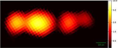
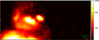
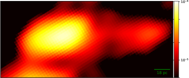
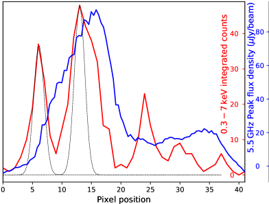
Figure 8: From top to bottom: S 10 jet in X-rays ($0.3-7\,\text{keV}$; scalebar in units of counts), H$\alpha$ line (scalebar in units of ADU for the VLT/FORS2 CCD), and 5.5 GHz band (scalebar in units of Jy beam^-1), rotated to a horizontal position; and corresponding brightness distribution along the jet in X-rays (red curve) and radio (blue curve), on the same spatial scale. For the bottom panel, we measured the X-ray brightness by integrating the pixel counts in 1-pixel-wide strips perpendicular to the jet axis; we measured the radio intensity from the peak value along the jet. The dotted black line represents a symmetric Gaussian approximation of the Chandra PSF of a point-like source at the location of S 10, determined from our PSF modelling (Section 3.1). At the distance of 1.88 Mpc, 1 ACIS-I pixel corresponds to $\approx$4.5 pc. The comparison shows that the second X-ray knot is extended and likely composed of (at least) two distinct sources, displaced by $\approx$1$.^{\prime\prime}$2 along the direction of the jet. For comparison, we show that the first knot instead matches the Chandra PSF.

The presence of multiple thermal X-ray knots rather than only two termination hot spots is the main difference between NGC 300 S 10 (Figure 8) and NGC 7793 S 26 (Soria et al., 2010). In this section, we outline possible scenarios that can give rise to a string of bright knots along the jet.

(i) Discrete relativistic ejecta:
Numerous compact accreting sources produce large-scale moving jets in the form of discrete ejecta. Ejection of relativistic plasma knots that emit via synchrotron processes have been observed at radio and X-ray wavelengths in the sub-Eddington low-mass X-ray binaries (LMXBs) H1743-322 (Corbel et al., 2005), XTE J1550-564 (Corbel et al., 2002; Kaaret et al., 2003) and XTE J1752-223 (Ratti et al., 2012). On the super-Eddington side, the ULX Ho II X-1 shows evidence of multiple discrete radio ejecta (Cseh et al., 2014). While each of the Ho II X-1 knots are not detected in X-rays, the S 10 jet could be made up of similar discrete ejecta where each southeast-northwest knot pair is due to a flare or outburst. In this scenario, the most recent ejecta would be the two unresolved blobs that constitute knot 2; the previous outburst would have produced knots 1 and 3; knot 4 would be the oldest ejection event whose southeastern counterpart has since faded (Figure 8). However, we rule out this scenario as the X-ray knots would have to be radiating via synchrotron emission, not thermally as we see for S 10.

(ii) Internal shocks:
The multiple-knot morphology may be a result of internal shocks within the jet (Rees & Meszaros, 1994; Malzac, 2014). Faster-moving ejecta catch up to slower-moving, previously ejected material further downstream, the collision causing shocks and accelerating particles. This would make S 10 analogous to the AGN jets we see in M87 (Rees, 1978; Sparks et al., 1996) and 3C 264 (Meyer et al., 2015). As with the previous scenario, internal shocks would produce synchrotron emission in the X-ray band and thus we can rule out this interpretation.

(iii) Multiple layers of ISM:
If instead we are looking at a more steady, continuous jet, with a persistent flow, then the additional knots could be explained by the jet punching through different layers of the ISM. The jet may be passing through shells of denser ISM, shocking the gas as it penetrates each layer. The resulting shocked gas would produce thermal X-ray emission. These over-densities in the ISM may simply be a result of random fluctuations in the ISM, or could be shells of material ejected by the massive progenitor either via stellar winds, or in giant eruptions, or during the SN explosion that produced the compact object. Nebulae around even the most powerful Luminous Blue Variable (LBV) stars are $\lesssim$ a few pc in size (Weis, 2011), an order of magnitude smaller than the size of the jet in S 10. However, the presence of numerous OB stars and likely SNRs in the nearby H ii region H 10 leaves open the possibility that stellar activity created supershells and filaments in the ISM on scales of $\sim$100 pc.

(iv) Multiple outbursts:
The accretion rate and/or the kinetic power carried by the jet may not be steady; the system may undergo state transitions. This could also be the reason for the current low X-ray luminosity of the core (further discussed in Section 4.4). If this is the case, then we do not expect a continuous jet, but rather phases of enhanced activity. Recurrent outbursts may be creating pairs of hotspots in a Sedov-Taylor phase that keep expanding and cooling as they propagate out from the central object. In between outbursts, the channel drilled by the jet during the previous phase of activity would be refilled by the ISM. The innermost X-ray hotspots, that is the two marginally resolved sources that form Chandra knot 2, would be those created during the most recent epoch of jet activity. The uneven number of knots may be due to an over density to the east of S 10 resulting in a pile-up of multiple knots. In AGN, a similar scenario of intermittent activity has been proposed to explain the so called “double-double radio galaxies”, characterised by multiple pairs of hot spots (often aligned along the same direction) sharing the same core (Schoenmakers et al., 2000; Kaiser et al., 2000; Saikia & Jamrozy, 2009; Brocksopp et al., 2011). In this scenario, NGC 300 S 10 would be the first unambiguous example of a double-double microquasar.

The fading and/or appearance of new knots would undoubtedly result in X-ray variability. Two or three major episodes of enhanced activity over a timescale of a few 10⁵ yr correspond to a recurrence timescale too long to be explained by thermal-viscous accretion disk instabilities, for a stellar-mass compact object. It is instead consistent, for example, with the timescale of thermal pulsations in an AGB donor star (e.g., Marigo et al., 2013), or of giant eruptions in LBV stars and other types of SN impostors (e.g.,  Smith & Owocki, 2006; Berger et al., 2009; Tartaglia et al., 2015). In particular, if the massive star is in a binary system with a neutron star or a black hole, giant eruptions are expected to produce phases of highly super-Eddington mass transfer onto the compact object, and may trigger powerful episodes of jet activity. This scenario was used to explain the behaviour of a transient neutron star ULX (coincidentally also located in NGC 300) associated with the SN impostor 2010da (e.g.,  Binder et al., 2016; Villar et al., 2016; Carpano et al., 2018). One of the hallmarks of such a scenario is that the erupting donor star would be surrounded by thick circumstellar dust, and would appear highly reddened (e.g.,  Berger et al., 2009; Lau et al., 2016). We mentioned earlier (Section 3.3.2) that one of the candidate optical counterparts, star D, is indeed highly reddened. We leave a detailed investigation of this possibility to further work.

(v) Sheath-spine jet:
A stratified jet has previously been used to explain the emission from gamma-ray bursts (GRBs) (Mészáros & Rees, 2001; Ramirez-Ruiz et al., 2002; Vlahakis et al., 2003). Known as a ‘spine-sheath’ jet model, a fast moving core (spine) is surrounded by a slower moving outflow (sheath) (see Fig 1. in Ito et al. 2013). This is thought to result from the GRB jet punching through the progenitor envelope, entraining the material to create the sheath (Mészáros & Rees, 2001; Ramirez-Ruiz et al., 2002), or from a decoupled neutron sheath and proton jet core (Vlahakis et al., 2003). For S 10, we do not expect direct emission from the jet, but instead suggest that a similar stratified jet may be causing multiple hotspots via external shocks. As the jet propagates out, the slower moving outer layer (or layers) shock the ISM, creating the inner knots, while the faster moving core punches through, decelerating further downstream, creating the outer knots.

We cannot discriminate between interpretations iii–v based on our current observations. Differentiating between a persistent or transient jet is important because it will help us identify the true power of S 10. In the following section we attempt to estimate the time averaged jet power. However, if the jet does switch on and off, then our jet power will be a lower limit; because we do not know the duty cycle of S 10, we cannot determine the instantaneous power of the jet.

4.3 Jet power

While S 10 has a unique morphology among Galactic and extragalactic stellar-mass objects, we relate it most closely to super-Eddington microquasars and ULXs such as SS 433, S 26 and Ho II X-1. These sources all demonstrate the presence of powerful jets either through radio/X-ray knots, shocked emission from jet/ISM interactions and/or extended radio nebulae. S 10 has a 5.5 GHz radio luminosity $L_{\rm 5.5\,GHz}\approx 1\times 10^{34}\,\text{erg s${}^{-1}$}$, which is a factor of two greater than the radio luminosity seen in the SS 433/W 50 complex (Downes et al., 1986; Dubner et al., 1998). On the other hand, it is an order of magnitude less radio luminous than the microquasars NGC 7793 S 26 (Soria et al., 2010)) and M 83 MQ1 (Soria et al., 2014). The physical size of the radio nebula of S 10 ($\approx 170\times 55\,\text{pc}$) is also comparable to the bubbles of S 26 ($\sim 300\times 150\,\text{pc}$; Soria et al. 2010), Ho II X-1 ($\sim 81\times 40\,\text{pc}$; Cseh et al. 2012) and SS 433 ($\sim 100\times 50\,\text{pc}$; Dubner et al. 1998). Thus, in this section, we primarily compare S 10 to these super-Eddington sources and their jet-inflated radio nebulae.

Assuming equipartion between the magnetic field and energy in relativistic particles, we can determine the minimum energy conditions for synchrotron radiation. The minimum energy $W_{\rm min}$ can be expressed as

$$W_{\rm min}\approx 3.0\times 10^{13}\eta^{4/7}V^{3/7}\nu^{2/7}L_{\nu}^{4/7}\,\text{erg},$$ (1)

(Longair, 2011) where $\eta-1$ is the ratio of energy in baryons to that in relativistic electrons, $V$ is the bubble volume in m³, $\nu$ is the observing frequency in Hz and $L_{\nu}$ is the luminosity density in $\text{W}\,\text{Hz}^{-1}$. The elongated structure of S 10 has dimensions of $\approx 170\times 55\,\text{pc}$. If we assume a cylindrical shape, this equates to a total volume of $\approx 10^{55}\,\text{m}^{3}$. Using this, and our 5.5 GHz luminosity density of $L_{\nu}=2.2\times 10^{17}\,\text{W}\,\text{Hz}^{-1}$, we calculate a synchrotron minimum-energy condition $W_{\rm min}=5.5\times 10^{49}\eta^{4/7}\,\text{erg}$ corresponding to a minimum magnetic field strength of $B_{\rm min}=7\,\mu\text{G}$. This is comparable to the minimum energies required to power the extended radio nebulae in other super-Eddington microquasars, such as NGC 5408 X-1 ($\sim$10⁴⁹ erg: Lang et al. 2007; or $\sim$10⁵⁰ erg: Soria et al. 2006, depending on different assumptions for the electron energy distribution), IC 342 X-1 ($\approx 9.2\times 10^{50}\text{erg}$: Cseh et al. 2012), and Ho II X-1 ($\approx 2.6\times 10^{49}\text{erg}$: Cseh et al. 2012). However, we note that there are several unknowns associated with our analysis. Firstly, without the viewing angle, we can only estimate the volume of the radio bubble based on its shape projected on the sky. The filling factor of the magnetic field throughout the bubble is also unknown. Additionally, the uncertainty on the minimum and maximum energy of the electron population, and therefore on the spectral index above and below the ATCA observing bands, also contribute to the uncertainty of the minimum-energy estimate.

We can estimate the jet power using the method outlined by Pakull et al. (2010). For a shock-ionized gas bubble, we know from standard theory (Weaver et al., 1977) that the total radiative luminosity $L_{\rm rad}$ is $\approx$27/77 of the mechanical power that is inflating the bubble. The total radiative luminosity of the cooling plasma can be determined from the luminosity in suitable diagnostic lines; for example, the H$\beta$ line emission (derived from Equations 2.2 and 2.4 of Dopita & Sutherland 1995, or from the shock-ionization code mappings v: Allen et al. 2008) is a good proxy for the total luminosity, because its relative contribution does not depend too strongly on the shock velocity, or the metallicity of the shocked gas, or the density of the undisturbed ISM. For a plausible range of shock velocities $\approx$150–300 km s^-1, the total H$\beta$ luminosity of shocked gas plus precursor is $\approx$(2–3)$\times 10^{-3}$ times the input mechanical power. For an H$\beta$ luminosity $L_{H\beta}\approx(6\pm 1)\times 10^{36}$ erg s^-1, this corresponds to a long-term-average jet power $P_{\rm kin}\approx$ (2–3) $\times 10^{39}$ erg s^-1, an order of magnitude lower than the values estimated for S 26 but the same order of magnitude as the jet power suggested for SS 433 (Brinkmann & Kawai, 2000; Marshall et al., 2002b; Krivosheyev et al., 2009) and for M 51 ULX-1 (Urquhart et al., 2018). In a follow-up paper currently in preparation, we will refine and improve this estimate of jet power based on diagnostic line emission, using recently obtained data from the Multi Unit Spectroscopic Explorer (MUSE), an integral field spectrograph mounted on the VLT.

Other techniques have sometimes been used to estimate the kinetic power in radio/optical microquasar bubbles (Pakull et al., 2010). If the shock velocity is known (inferred from optical spectroscopic studies of the emission line profiles), together with the ISM density and the bubble size, one can derive the characteristic dynamical age of the shocked bubble as well as the jet power (Weaver et al., 1977). A spectroscopic study of the optical emission lines in S 10 is also left to our follow-up paper based on MUSE data. A much less reliable technique is based on the radio luminosity. Various scalings between the jet power and the optically thin synchrotron luminosity of hot spots, lobes and cavities have been proposed, for samples of radio galaxies (e.g.,  Willott et al., 1999; Cavagnolo et al., 2010; Godfrey & Shabala, 2013). The model assumptions underpinning these scaling relations are similar to those associated with the minimum energy synchrotron conditions discussed earlier, leading to a similar degree of uncertainty. However, Godfrey & Shabala (2016) have shown that the scaling relations commonly used in the literature are strongly biased by the mutual dependence on distance for both the jet power and the radio luminosity. Thus, we do not rely on those correlations for our study.

4.4 Synchrotron or thermal plasma emission?

From the synchrotron minimum energy conditions, we can estimate the cooling timescale for X-ray synchrotron emission. At an energy of 1 keV, the cooling timescale would be $3,000\left(\frac{B_{\rm min}}{7\,\mu\text{G}}\right)^{-3/2}\,\text{yr}$ (Tudose et al., 2006). This approximation is valid if the system is in equipartition; a stronger magnetic field will reduce the cooling timescale. Adiabatic expansion of the knots would also lead to faster cooling.

Based on the $5.5\,\text{GHz}$ luminosity and average spectral index ($\alpha=-0.64$) for the radio bubble, the expected $0.3-8.0\,\text{keV}$ X-ray synchrotron luminosity is $\approx 3\times 10^{37}\,\text{erg s${}^{-1}$}$. We have already tested (Section 3.1.1) that a power-law component with a photon index $\Gamma=1.7$ does not provide a statistically significant contribution to the combined knot spectrum, and the 90% upper limit to its luminosity is $<2\times 10^{36}\,\text{erg s${}^{-1}$}$. For completeness, given the spectral index found in the radio analysis (Section 3.2) and that we now suspect the microquasar candidate core resides within X-ray knot 2 (Section 3.1.2), we perform the test with an X-ray power-law component of photon index $\Gamma=1.64$ on the individual spectrum of knot 2. As expected, the result is essentially identical to the case for the combined spectra and for $\Gamma=1.7$, that is there is no statistically significant need for such a component, and the 90% upper limit to its contribution is $<8\times 10^{35}\,\text{erg s${}^{-1}$}$. This is lower than the luminosity expected from the extrapolation of the radio synchrotron power law. The reason why we do not see synchrotron X-ray emission may be that particles were never accelerated up to energies where they could emit X-rays via this process; or there may be a break in the spectrum between radio and X-ray frequencies because of ageing. We also note that the radio and X-ray observations were not simultaneous. Alternatively, the S 10 core may be producing X-ray synchrotron emission that is strongly absorbed to the point where it is not detected. While the thermal X-ray emission does not show any evidence of strong absorption, it is likely a result of extended jet/ISM interactions, whereas the X-ray synchrotron emission must emanate from a region much closer to the compact object and could be obscured by an additional strong source of absorption; $n_{\rm H}>4\times 10^{23}$ atoms cm^-2. This scenario seems somewhat contrived and thus we prefer the simpler interpretation wherein the synchrotron power-law has a break below the soft X-ray band, in line with other microquasars (Russell et al., 2013a), and both the radio synchrotron and the X-ray thermal emission come from similar regions of jet/ISM interactions.

While we do not detect any X-ray synchrotron emission, we do see thermal X-ray emission (Bremsstrahlung and line transitions), likely from shock-heated gas along and in front of the jet. The cooling timescale is approximately the ratio of total heat content over heat loss rate

$$t_{\rm cool}=\frac{3(n_{\rm e}+n)k_{\rm B}T}{2n^{2}\Lambda},$$ (2)

(Dopita & Sutherland, 2003) where $n$ is the atomic density of the hot gas, $k_{\rm B}$ is the Boltzmann constant, $T$ is the plasma temperature and $\Lambda$ is the cooling function. From our X-ray spectral fits, we know that $T\approx 0.6\,\text{keV}\approx 7\times 10^{6}\,\text{K}$. At that temperature, $\Lambda\approx 4\times 10^{-23}$ erg cm³ s^-1 for solar-metallicity plasma in collisional equilibrium, including both free-free and line emission (Sutherland & Dopita, 1993). From the thermal X-ray luminosity and the approximate volume estimated for the emitting gas, we also determined a lower limit on the density, $n\approx n_{e}\gtrsim 4\,\text{c}\text{m}^{-3}$ (Section 3.1.1). Putting those constraints together, we obtain an upper limit on the (thermal) cooling timescale of $t_{\rm cool}\lesssim 570,000\,$yr. We speculate that X-ray-emitting gas is replenished by bursts of increased accretion/ejection activity leading to the production of new discrete knots on a recurrence timescale shorter than the cooling timescale.

4.5 Faintness of the X-ray core

Three possibly super-Eddington microquasars have been found so far with large-scale X-ray evidence of collimated jets: NGC 300 S 10, NGC 7793 S 26 and SS 433 in the Milky Way. Curiously, all three have apparently faint cores: $L_{\rm{X,core}}\lesssim 10^{36}$ erg s^-1 (Section 3.1.2), $L_{\rm{X,core}}\approx 6\times 10^{36}\,\text{erg s${}^{-1}$}$ (Soria et al., 2010) and $\sim 10^{36}\,\text{erg s${}^{-1}$}$ (Kotani et al., 1996; Fabrika & Medvedev, 2011) for the three sources, respectively. In the case of SS 433, the reason is the occultation of the direct X-ray emission by the thick super-critical disk, seen at high inclination (Fabrika, 2004). For S 26 and S 10, we do not have any estimate of the viewing angle. No firm conclusions can be reached based on such a small sample of objects. It is possible that there is a selection bias at play: large-scale jets appear longer and easier to discover when they are in the plane of the sky; as a result, the accretion disk around the compact object would preferentially appear edge-on. The situation would be analogous to that of “accretion disk corona” sources, a type of Galactic low-mass X-ray binary seen at high inclination, in which the direct X-ray emission from the disk surface is mostly occulted from us, and we can only see harder radiation scattered by a vertically extended corona (e.g.,  White & Holt, 1982; McClintock et al., 1982; Hellier & Mason, 1989). Alternatively, the compact object may be faint because its super-critical accretion phase has a short duration compared with the cooling timescale of the hot spots and bubble, or it is a transient source with a low duty cycle. Contrary to this scenario, it was noted (Pakull & Grisé, 2008) that the majority of large shock-ionized ULX bubbles (without direct evidence of a collimated jet) do contain a luminous X-ray core; if the typical duty cycle of super-Eddington accretors was low, or if the duration of the super-Eddington phase was much shorter than the cooling timescale of the ULX bubbles, we would see a large number of bubbles without a central source, which is not the case .

We can take the low-duty-cycle argument to an extreme, and suggest that all the kinetic power in the collimated jet was injected at an instantaneous burst event, for example a SN associated with a Gamma-Ray-Burst (GRB). After that event, the collimated ejecta would continue to expand passively, now dominated by entrained material from the ISM. This scenario leads us back to the original interpretation of S 10 as an SNR. Magneto-hydrodynamical simulations of jet/ISM interactions in GRBs suggest (De Colle et al., 2012) that the jet loses collimation at a distance of $\sim$1 pc from the origin; this makes it difficult to explain the much larger length of the S 10 structure. To test this scenario further, we searched for evidence of current accretion activity at the (candidate) location of the central object, as explained in the next section.

4.6 Search for X-ray and radio variability

Spurred by the possibility that the central engine of S 10 is a transient or variable accretor, currently in a low state, we searched for hints of previous variability in the core emission. S 10 has been observed on several occasions with the ROSAT and the XMM Newton X-ray telescopes: in both cases, the source was not resolved, because of their poorer spatial resolution (see, e.g., Figures 8e and 8f in Payne et al. 2004). For the ROSAT observations, we used the count rates listed in the Second Position-Sensitive Proportional Counter (PSPC) Catalog (Rosat, 2000) and in the Source Catalog of Pointed Observations with the High Resolution Imager (HRI) (ROSAT Scientific Team, 2000). For the XMM-Newton observations, we used the observed fluxes from the 3XMM-Data Release 6 Catalog (Rosen, 2016). We then used the online tool PIMMS version 4.8e to convert the count rates or fluxes of the various observations to unabsorbed 0.3–8 keV fluxes and then to luminosities, assuming a $0.6\,\text{keV}$ thermal plasma model and a column density of $n_{\rm H}=3\times 10^{20}\,\text{c}\text{m}^{3}$, as for our spectral modelling (Section 3.1, Table 5).

For the ROSAT/PSPC observations between 1991 November and 1992 January, we estimate a luminosity $L_{0.3-8}=(1.3\pm 0.3)\times 10^{37}$ erg s^-1; for the PSPC observations between 1992 May–June, $L_{0.3-8}=(1.1\pm 0.2)\times 10^{37}$ erg s^-1. For the ROSAT/HRI observation in 1995 May, we obtain a luminosity $L_{0.3-8}=(1.5\pm 0.4)\times 10^{37}$ erg s^-1. Finally, XMM-Newton observed NGC 300 between 2000 December and 2001 January; the absorbed 0.2–12 keV flux of $(3.44\pm 0.13)\times 10^{-14}$ erg cm^-2 s^-1 converts to an emitted 0.3–8 keV luminosity $L_{0.3-8}=(1.6\pm 0.2)\times 10^{37}$ erg s^-1. Considering the model uncertainties and the differences between the PSFs and energy bands of the various detectors, we cannot claim any significant X-ray variability compared with our modelled Chandra luminosity $L_{0.3-8}=(1.1\pm 0.1)\times 10^{37}$ erg s^-1 (average of the 2010 and 2014 observations). Any possible variability of the core was swamped by the higher and constant thermal emission from the various knots.

Table 8: Integrated radio flux of the core region at various epochs.

Telescope	Year	$\nu$	Flux density	$\nu L_{\nu}$
		(GHz)	(mJy)	($10^{33}\,\text{erg s${}^{-1}$}$)
ATCA	2000-02-28	1.374	$0.56\pm 0.03$	3.3
ATCA	2000-02-28	2.496	$0.38\pm 0.06$	4.0
ATCA∗	2015/16	5.5	$0.429\pm 0.030$	10.0
ATCA∗	2015/16	9.0	$0.352\pm 0.029$	13.4

^∗ ATCA observations from this study (October 2015 and August 2016) are stacked as per Section 2.2.

We then checked whether S 10 has varied in radio brightness over the last decades. NGC 300 was observed with the VLA at $4.885\,\text{GHz}$ in May 1993 and at $1.465\,\text{GHz}$ in June 1998 (Pannuti et al., 2000). It was also observed with the ATCA in February 2000 at $1.374\,\text{GHz}$ and $2.496\,\text{GHz}$ (Payne et al., 2004). We compared these data with our recent 2016–2017 ATCA observations. One major difficulty in this comparison is that the archival data have larger beam sizes: $6^{\prime\prime}\times 6^{\prime\prime}$ for the old ATCA observations, $4^{\prime\prime}.70\times 3^{\prime\prime}.76$ for the 1.465 GHz VLA observations, and $8^{\prime\prime}.63\times 4^{\prime\prime}.22$ for the 4.885 GHz VLA observations (Table 2 in Payne et al. 2004). This makes it difficult to distinguish between the radio flux from the S 10 jet and that from the neighbouring H 10 Hii region. The second major problem is that the archival observations were much less sensitive. The rms noise level was $\sigma\approx 37\mu$Jy beam^-1 and $\sigma\approx 66\mu$Jy beam^-1 for the VLA data at $4.885\,\text{GHz}$ and at $1.465\,\text{GHz}$, respectively; for the archival ATCA data it was $\sigma\approx 58\mu$Jy beam^-1 and $\sigma\approx 62\mu$Jy beam^-1 at $1.374\,\text{GHz}$ and $2.496\,\text{GHz}$, respectively. As a comparison, the rms noise was $\sigma\approx 2.7\mu$Jy beam^-1 in the 2015–2017 ATCA data (Section 2.2). As a result, the emission from the core region (around the X-ray knot 2) is the only part of the radio jet that is significantly detected in the archival data (see for example Fig. 8d of Payne et al. 2004). Keeping in mind all these caveats, and extrapolating the 2015–2016 flux measurements to lower frequencies using a spectral index $\alpha=-0.40\pm 0.22$ for the core region, we find that the new ATCA flux measurements are consistent with the 2000 ATCA flux values within $\approx$2$\sigma$. Instead, when compared with the VLA flux densities measured by Pannuti et al. (2000) and Payne et al. (2004), S 10 appears to have brightened by a factor of 2 in the ATCA observations; however, our re-analysis of the VLA data shows that the true uncertainties in the S 10 core flux are much larger than the formal error reported by Pannuti et al. (2000) and Payne et al. (2004), because of the mismatch in beam size and sensitivity mentioned above. To combat this, and properly compare the S 10 core fluxes, we re-analysed both the 4.8 GHz VLA data and our 5.5 GHz ATCA data. These observations were chosen to minimise uncertainties introduced by the spectral shape of S 10. Additionally, we applied the same uv-cut to both data sets and used the same restoring beam. We find peak fluxes of $f_{4.8\,\text{GHz}}=340\pm 60\,\text{$\mu$}\text{Jy}\,$$\,{\rm beam}^{-1}$and $f_{5.5\,\text{GHz}}=210\pm 8\,\text{$\mu$}\text{Jy}\,$$\,{\rm beam}^{-1}$. We find tentative evidence ($\sim 2\sigma$) of a decrease in the flux of the radio core, though future observations are required to conclusively establish the presence of variability.

5 Conclusions

We have presented a new, coherent interpretation of a complex X-ray, optical and radio source in NGC 300, using new and archival Chandra, HST, VLT and ATCA data. The source was previously classified as an SNR; however, we argued that it is a candidate microquasar, likely powered by super-Eddington accretion onto a compact object. We showed that the X-ray emission is made of a string of discrete knots, a tell-tale sign of a jet interacting with the ambient medium. We also showed for the first time that the radio emission is an elongated bubble ($\approx$170 $\times 55$ pc in size), oriented along the same direction as the string of X-ray knots. While the radio emission is consistent with optically-thin synchrotron (as expected), the X-ray emission is from thermal plasma at temperatures $\approx$0.3–0.8 keV. This is unlike the knots and hot spots typically seen in AGN jets, but is analogous to the thermal hot spots previously identified in the super-Eddington microquasar NGC 7793 S 26. The integrated radio luminosity at 5.5 GHz is $\approx$10³⁴ erg s^-1, while the total X-ray luminosity of the knots is $\approx$2 $\times 10^{37}$ erg s^-1. To complete the picture, we argued that the optical line spectrum of the shock-ionized nebula is exactly what is expected for this kind of system, as seen also in S 26 and in other shock-ionized ULX bubbles. In particular, we showed a spatial association between locations of enhanced H$\alpha$ emission and locations of X-ray and radio features.

Using the H$\alpha$ line luminosity ($L_{H\alpha}\approx 1.7\times 10^{37}$ erg s^-1) as a proxy, we estimated that the nebula was shocked by the injection of a long-term-average jet power $P_{\rm{kin}}\approx$ (2–3) $\times 10^{39}$ erg s^-1. Thus, this candidate microquasar is in the same energy class as SS 433 and Ho II X-1; it is an order of magnitude less energetic and a factor of 2 smaller in linear size than S 26.

We have discussed the most likely location of the core, but found no bright, point-like X-ray source there, above the thermal-plasma emission. The upper limit to the X-ray luminosity of the core is $\approx$10³⁶ erg s^-1. The direct emission from the accreting compact object may be occulted from our view by a thick, edge-on disk, like in SS 433; or the core could be in a low state. Neither did we find evidence of a brighter core in earlier XMM-Newton and ROSAT observations, which stretch back to 1991. The reason for the multiple knot structure remains unclear. We can rule out internal shocks (analogous to the knots seen for example in the M 87 jet), because the X-ray emission is thermal (that is, from shocked ISM) rather than synchrotron. For the same reason, we consider very unlikely that the knots are ballistic ejections. We discussed alternative scenarios, in particular: multiple layers of enhanced ISM density; multiple outbursts or jet activity episodes; or a sheath-spine jet structure, with the faster spine propagating a longer distance than the slower sheath.

In summary, S 10 is a key object to understand jets in the super-critical accretion regime, and is an ideal source for follow-up multiwavelength observations. The most important piece of information that we are missing is the shock velocity of the optically-emitting gas, including possible velocity differences between the plasma above and below the core position. This would provide us with a dynamical age of the bubble and an alternative measurement for the mechanical power. We will tackle this problem in follow-up work currently in preparation, based on recently obtained MUSE data; thanks to those new results, we will be able to directly compare the estimates of jet power inferred from the kinematics of the shocked gas, and from the optical line fluxes. Increasing the sample size of super-Eddington microquasars (and, more generally, of shock-ionized ULX bubbles) is crucial for our understanding of jet launching and collimation processes, and energy feedback.

References

- Alexander et al. (2016) Alexander K. D., Berger E., Guillochon J., Zauderer B. A., Williams P. K. G., 2016, ApJ, 819, L25
- Allen et al. (2006) Allen S. W., Dunn R. J. H., Fabian A. C., Taylor G. B., Reynolds C. S., 2006, MNRAS, 372, 21
- Allen et al. (2008) Allen M. G., Groves B. A., Dopita M. A., Sutherland R. S., Kewley L. J., 2008, ApJS, 178, 20
- Arnaud (1996) Arnaud K. A., 1996, in Jacoby G. H., Barnes J., eds, Astronomical Society of the Pacific Conference Series Vol. 101, Astronomical Data Analysis Software and Systems V. p. 17
- Begelman et al. (1984) Begelman M. C., Blandford R. D., Rees M. J., 1984, Reviews of Modern Physics, 56, 255
- Berger et al. (2009) Berger E., et al., 2009, ApJ, 699, 1850
- Binder et al. (2016) Binder B., Williams B. F., Kong A. K. H., Gaetz T. J., Plucinsky P. P., Skillman E. D., Dolphin A., 2016, MNRAS, 457, 1636
- Blair & Long (1997) Blair W. P., Long K. S., 1997, ApJS, 108, 261
- Blandford & Payne (1982) Blandford R. D., Payne D. G., 1982, MNRAS, 199, 883
- Blandford & Znajek (1977) Blandford R. D., Znajek R. L., 1977, MNRAS, 179, 433
- Bressan et al. (2012) Bressan A., Marigo P., Girardi L., Salasnich B., Dal Cero C., Rubele S., Nanni A., 2012, MNRAS, 427, 127
- Brinkmann & Kawai (2000) Brinkmann W., Kawai N., 2000, A&A, 363, 640
- Brinkmann et al. (2007) Brinkmann W., Pratt G. W., Rohr S., Kawai N., Burwitz V., 2007, A&A, 463, 611
- Brocksopp et al. (2011) Brocksopp C., Kaiser C. R., Schoenmakers A. P., de Bruyn A. G., 2011, MNRAS, 410, 484
- Carpano et al. (2018) Carpano S., Haberl F., Maitra C., Vasilopoulos G., 2018, MNRAS, 476, L45
- Cash (1979) Cash W., 1979, ApJ, 228, 939
- Cavagnolo et al. (2010) Cavagnolo K. W., McNamara B. R., Nulsen P. E. J., Carilli C. L., Jones C., Bîrzan L., 2010, ApJ, 720, 1066
- Chen et al. (2015) Chen Y., Bressan A., Girardi L., Marigo P., Kong X., Lanza A., 2015, MNRAS, 452, 1068
- Corbel et al. (2002) Corbel S., Fender R. P., Tzioumis A. K., Tomsick J. A., Orosz J. A., Miller J. M., Wijnands R., Kaaret P., 2002, Science, 298, 196
- Corbel et al. (2005) Corbel S., Kaaret P., Fender R. P., Tzioumis A. K., Tomsick J. A., Orosz J. A., 2005, ApJ, 632, 504
- Coughlin & Begelman (2014) Coughlin E. R., Begelman M. C., 2014, ApJ, 781, 82
- Cseh et al. (2012) Cseh D., et al., 2012, ApJ, 749, 17
- Cseh et al. (2014) Cseh D., et al., 2014, MNRAS, 439, L1
- Cseh et al. (2015) Cseh D., et al., 2015, MNRAS, 452, 24
- D’Odorico et al. (1978) D’Odorico S., Benvenuti P., Sabbadin F., 1978, A&A, 63, 63
- D’Odorico et al. (1980) D’Odorico S., Dopita M. A., Benvenuti P., 1980, A&AS, 40, 67
- De Colle et al. (2012) De Colle F., Ramirez-Ruiz E., Granot J., Lopez-Camara D., 2012, ApJ, 751, 57
- Dickey & Lockman (1990) Dickey J. M., Lockman F. J., 1990, ARA&A, 28, 215
- Dopita & Sutherland (1995) Dopita M. A., Sutherland R. S., 1995, ApJ, 455, 468