Hydrodynamics of circumbinary accretion: angular momentum transfer and binary orbital evolution

Abstract

We carry out 2D viscous hydrodynamical simulations of circumbinary accretion using the moving-mesh code AREPO. We self-consistently compute the accretion flow over a wide range of spatial scales, from the circumbinary disk (CBD) far from the central binary, through accretion streamers, to the disks around individual binary components, resolving the flow down to $2\%$ of the binary separation. We focus on equal-mass binaries with arbitrary eccentricities. We evolve the flow over long (viscous) timescales until a quasi-steady state is reached, in which the mass supply rate at large distances ${\dot{M\mkern 3.0mu}\mkern-3.0mu}{}_{0}$ (assumed constant) equals the time-averaged mass transfer rate across the disk and the total mass accretion rate onto the binary components. This quasi-steady state allows us to compute the secular angular momentum transfer rate onto the binary, $\langle{\dot{J\mkern 3.0mu}\mkern-3.0mu}{}_{\rm b}\rangle$, and the resulting orbital evolution. Through direct computation of the gravitational and accretional torques on the binary, we find that $\langle{\dot{J\mkern 3.0mu}\mkern-3.0mu}{}_{\rm b}\rangle$ is consistently positive (i.e., the binary gains angular momentum), with $l_{0}\equiv\langle{\dot{J\mkern 3.0mu}\mkern-3.0mu}{}_{\rm b}\rangle/{\dot{M\mkern 3.0mu}\mkern-3.0mu}{}_{0}$ in the range of $(0.4-0.8)a_{\rm b}^{2}\Omega_{\rm b}$, depending on the binary eccentricity (where $a_{\rm b},~{}\Omega_{\rm b}$ are the binary semi-major axis and angular frequency); we also find that this $\langle{\dot{J\mkern 3.0mu}\mkern-3.0mu}{}_{\rm b}\rangle$ is equal to the net angular momentum current across the CBD, indicating that global angular momentum balance is achieved in our simulations. In addition, we compute the time-averaged rate of change of the binary orbital energy for eccentric binaries, and thus obtain the secular rates $\langle\dot{a}_{\rm b}\rangle$ and $\langle\dot{e}_{\rm b}\rangle$. In all cases, $\langle\dot{a}_{\rm b}\rangle$ is positive, i.e., the binary expands while accreting. We discuss the implications of our results for the merger of supermassive binary black holes and for the formation of close stellar binaries.

1. Introduction

Circumbinary accretion disks are a natural byproduct of binary star formation via disk fragmentation (e.g., Boss, 1986; Bonnell & Bate, 1994a, b; Kratter et al., 2008). A number of these disks have been observed around Class I/II young stellar binaries – well known objects include GG Tau, DQ Tau and UZ Tau E (e.g. Dutrey et al., 1994; Mathieu et al., 1996, 1997) – and recently even around much younger binary Class 0 objects like L1448 IRS3B (Tobin et al., 2016). Circumbinary disks are also expected to form around massive binary black holes following galaxy mergers (e.g. Begelman et al., 1980; Milosavljević & Merritt, 2001; Milosavljević & Phinney, 2005; Escala et al., 2005; Mayer et al., 2007; Dotti et al., 2007; Cuadra et al., 2009; Chapon et al., 2013), and even from the fall-back ejecta around post-common envelope binaries (e.g., Kashi & Soker, 2011). The interaction between the two central bodies and the surrounding gas via accretion and gravitational torques dictates the long-term evolution of the binary orbit. Thus, understanding the details of binary-disk interaction is essential to explaining the end-state distribution of stellar binary properties, and to deciphering how, or if, a circumbinary disk (CBD) can assist the orbital decay of black hole binaries, initiating the process toward merger.

It is commonly assumed that the binary inevitably loses specific angular momentum by interacting with the outer disk/ring (e.g., Pringle, 1991), which results in the migration/coalescence of the binary toward smaller orbital separations. This reasoning follows from extending the classical theory of satellite-disk interaction for extreme mass ratios (e.g., Lin & Papaloizou, 1979; Goldreich & Tremaine, 1980; Lin & Papaloizou, 1986; Ward, 1997), into the regime of binaries (mass ratios of order unity): the binary and disk are coupled via Lindblad resonance torques, and since the CBD rotates at an angular frequency that is lower than the binary’s, the nonaxisymmetric perturbations exerted in the gas “lag” the binary, thus exerting a negative torque on it. Numerous studies (e.g., Gould & Rix, 2000; Armitage & Natarajan, 2002, 2005; Cuadra et al., 2009; Haiman et al., 2009; Chang et al., 2010; Farris et al., 2015; Rafikov, 2016; Kelley et al., 2017) have modeled the extraction of angular momentum from the binary by the outer disk, suggesting that a “gas-assisted” orbital migration may be important in facilitating binary black hole mergers at separations that are too wide for gravitational wave radiation to remove orbital angular momentum efficiently (what is known as the “final parsec” problem, Milosavljević & Merritt, 2003b, a).

Two complications can alter this picture of binary migration. The first, and most obvious, is that binaries can accrete from the CBD, and this must be taken into account when computing the torques exerted on the binary by the disk. Accretion torques and gravitational torques can be of a similar order of magnitude: the change in angular momentum by accretion alone is proportional to the mass accretion rate ${\dot{M\mkern 3.0mu}\mkern-3.0mu}{}$, while the gravitational Lindblad torque is proportional to the inner disk surface density, which is itself proportional to ${\dot{M\mkern 3.0mu}\mkern-3.0mu}{}$ provided that the disk is in a steady state. Because of the time-dependent forcing from the binary, it is only possible to reach a “quasi-steady state,” in which the time-averaged mass accretion rate onto the binary matches the mass transfer rate in the CBD. To achieve this quasi-steady state, simulations require a steady mass supply at large distances from the binary and a long integration time. Only under these conditions, can it be guaranteed that the (arbitrary) initial conditions have no impact in the torque balance of the system. Recently, Muñoz & Lai (2016) and Miranda et al. (2017) have shown such quasi-steady-state can indeed be achieved, at least when the disk viscosity is sufficiently large, in which case the CBD transfers, on average, the same amount of gas to the binary as it would to a single object. Thus, the deep cavity carved in the gas by the gravitational torques can only modulate (see Artymowicz & Lubow, 1996; Günther & Kley, 2002; MacFadyen & Milosavljević, 2008; Hanawa et al., 2010; de Val-Borro et al., 2011; Shi et al., 2012; D’Orazio et al., 2013; Farris et al., 2014; Shi & Krolik, 2015), but not suppress, the net accretion onto the binary (although see Ragusa et al., 2016, for a claim to the contrary at low viscosities). Numerical studies have shown that accretion can be modulated at either $\sim 5P_{\rm b}$ or $P_{\rm b}$ (the binary orbital period), and that the transition between these two regimes depends on the binary mass ratio (D’Orazio et al., 2013; Farris et al., 2014) or binary eccentricity, as shown by Muñoz & Lai (2016) and Miranda et al. (2017) (see also Artymowicz & Lubow, 1996; Hayasaki et al., 2007, for qualitatively similar results using smoothed particle hydrodynamics).

The second complication is the unexplored contribution of the “circum-single” disks (CSDs) to the total gravitational torque. In the same way that the outer CBD is expected to contribute negatively to the torque on the binary, the CSDs are expected to contribute positively (Goldreich & Tremaine, 1980), with the total torque consisting of the net balance of the inner and outer Lindblad torques (which is typically negative for mass ratios of $\lesssim 10^{-4}$; Ward, 1986, 1997). Savonije et al. (1994) computed the non-linear effect of the CSDs on the binary orbit in the large mass ratio ($\lesssim 1$) regime, concluding that the gas loses angular momentum to the binary, which results in wave-induced accretion onto the primary (see also Ostriker, 1994; Muñoz et al., 2015; Winter et al., 2018). Whether these inner/CSD torques can be of significance, or even compete with the outer CBD torque is an open, and largely unexplored, question.

In order to compute the full balance of torques, one needs to ($i$) resolve the gas dynamics well within the Roche lobes of the primary and secondary, and also ($ii$) guarantee that the numerical scheme is able to capture the non-linear response of the CSDs to the tidal forcing by the binary companions. These requirements can be met by shock-capturing hydrodynamical simulations at sufficiently high resolution. Recently, novel, Godunov-type numerical schemes with good shock-capturing properties – such as the DISCO (Duffell & MacFadyen, 2011) and AREPO (Springel, 2010; Pakmor et al., 2016) methods – have been used to compute the joint gas dynamical evolution of CBDs and CSDs down to small scales over a large number of binary orbits (Farris et al., 2014, 2015; Muñoz & Lai, 2016; Tang et al., 2017). Our simulations using AREPO (Muñoz & Lai, 2016) have uncovered several new features, of short-term ($\sim P_{\rm b}$) and long-term ($\sim 200P_{\rm b}$) variability, in the accretion rate onto eccentric binaries.

In a systematic exploratory work, Miranda et al. (2017) (hereafter MML17) simulated viscous disks around binaries with mass ratio ${\sim 1}$ and computed the net angular momentum transfer within a CBD as a function of radius in quasi-steady-state. They found that the net angular momentum transfer rate at the disk’s edge to be positive (i.e., angular momentum is transferred inward) for various values of the binary eccentricity. This implies that in quasi-steady-state, the binary gains angular momentum from the gas, possibly leading to binary expansion instead of coalescence. However, the work of MML17 is subject to an important limitation: the gas within the binary’s orbit was not simulated (see also MacFadyen & Milosavljević, 2008; D’Orazio et al., 2013). Although capturing a portion of the circumbinary cavity, the simulations of MML17 excluded the high-density region where the CSDs form, excising this region by imposing a diode-like boundary condition on an annulus of radius similar to the binary separation. As a consequence, the complex inflow-outflow nature of the gas inside the circumbinary cavity (Muñoz & Lai, 2016; Tang et al., 2017) was not captured correctly (this type of boundary may even be prone to some numerical artifacts; Thun et al., 2017). The purpose of the present work is to remove this limitation, by self-consistently computing the gas dynamics within the circumbinary cavity down to scales of $2\%$ of the binary separation, while simultaneously evolving a CBD that extends out to a distance of almost two orders of magnitude larger than the binary separation.

As in Muñoz & Lai (2016) (hereafter ML16), we use the moving-mesh code AREPO to simulate circumbinary accretion. We consider CBDs with a steady mass supply far from the binary. This supply is enforced in the form of a boundary condition (also implemented by MML17), which allows for the possibility of a global steady state, in which the time-averaged accretion rate onto the binary equals to the mass supply rate. We demonstrate through explicit computations, that in quasi-steady-state, the angular momentum transfer rate within the CBD equals the total torque (from gravitational forces and accretion) acting on the binary. This provides unambiguous evidence that the binary gains angular momentum from the CBD. Furthermore, by tracking the orbital energy and angular momentum of the accreting binary, we compute the combined orbit-eccentricity evolution of the binary for the first time on secular timescales.

This paper is organized as follows. In Section 2, we describe our use of moving-mesh hydrodynamics to simulate circumbinary accretion flows, and discuss how one can compute the various torques acting on the accreting binary. In Section 3, we describe and analyze our simulation results, identifying the similarities and differences between circular and eccentric binaries. In Section 4, we describe our calculation of the orbital energy and angular momentum changes, and we translate our results into orbital element evolution. Finally, in Section 5 we summarize our results and discuss the implications of this work for the formation and evolution of stellar binaries and supermassive binary black holes.

2. Numerical Methods

2.1. Moving-mesh Hydrodynamics

We carry out hydrodynamical simulations using the Godunov-type, moving-mesh code AREPO (Springel, 2010; Pakmor et al., 2016) in its Navier-Stokes version (Muñoz et al., 2013; Muñoz, 2013). AREPO has been implemented for viscous accretion disk simulations in 2D (Muñoz et al., 2014; ML16) and 3D (Muñoz et al., 2015). In the present work, we carry out circumbinary accretion simulations closely following the methodology of ML16. In brief, we simulate two-dimensional, Newtonian viscous flow, with a locally isothermal equation of state $P=\Sigma c_{s}^{2}$. The gravitational acceleration due to the binary’s potential $\Phi_{\rm b}(\mathbf{r})$ is evaluated at each cell center, and the motion of the moving cells by action of this external potential is integrated in a leapfrog-like fashion, i.e., gravity and pure hydrodynamics are “operator-split” (see Springel, 2010 and Pakmor et al., 2016). The positions of the primary and secondary, $\mathbf{r}_{1}(t)$ and $\mathbf{r}_{2}(t)$ respectively, as well as their velocities $\mathbf{v}_{1}(t)$ and $\mathbf{v}_{2}(t)$, are prescribed functions of time, determined at each $t$ by solving the Kepler equation given the binary eccentricity $e_{\rm b}$ and the mass ratio $q_{\rm b}=M_{2}/M_{1}$ (e.g Murray & Dermott, 2000). Both $e_{\rm b}$ and the binary semi-major axis $a_{\rm b}$ are fixed constants throughout the duration of the simulation. Such a “prescribed” binary is chosen over a “live” binary to minimize noise or high frequency “jittering” of the binary’s orbital elements. The sound speed $c_{s}(\mathbf{r})$ is a prescribed function of $\mathbf{r}$, and is fed into an iterative isothermal Riemann solver at each Voronoi cell interface (e.g., Toro, 2009; Springel, 2010). The temperature of the disk is set by the global parameter $h_{0}$, the disk’s vertical aspect ratio. Like the sound speed, the kinematic viscosity coefficient $\nu(\mathbf{r})$ is also a function of $\mathbf{r}$, and proportional to a Shakura-Sunyaev coefficient $\alpha$. The functions $c_{s}(\mathbf{r})$ and $\nu(\mathbf{r})$ are constructed such that $c_{s}^{2}\approx h_{0}^{2}\mathcal{G}(M_{1}+M_{2})/|\mathbf{r}|$ and $\nu\approx\alpha h_{0}^{2}\sqrt{\mathcal{G}(M_{1}+M_{2})|\mathbf{r}|}$ when $|\mathbf{r}|\gg a_{\rm b}$, and that $c_{s}^{2}\approx h_{0}^{2}\mathcal{G}M_{i}/|\mathbf{r}-\mathbf{r}_{i}|$ and $\nu\approx\alpha h_{0}^{2}\sqrt{\mathcal{G}M_{i}|\mathbf{r}-\mathbf{r}_{i}|}$ ($i=1,2$) when $|\mathbf{r}-\mathbf{r}_{i}|\ll a_{\rm b}$; i.e., both the CBD and the two CSDs behave like traditional $\alpha$-disks when the flow is approximately Keplerian (for more details, see ML16).

We allow the gas to be accreted by the individual members of the binary (from here on, we will refer to the binary components as “stars,” although the results presented here are equally applicable to black hole binaries). Accretion is thus carried out by a sink particle algorithm: as gas cells get closer than a critical distance $r_{\rm acc}$ to one of the stars, they are flagged for their contents to be drained (cells are not eliminated) at the end of the time step. In order to keep the transition at $|\mathbf{r}-\mathbf{r}_{i}|=r_{\rm acc}$ smooth and avoid severe depletion of cells (which can affect the convergence speed of the Voronoi tessellation algorithm), we accrete cells with $|\mathbf{r}-\mathbf{r}_{i}|\approx 0$ more aggressively than those with $|\mathbf{r}-\mathbf{r}_{i}|\approx r_{\rm acc}$. This is accomplished by using a smooth spline function (Springel et al., 2001) that returns the fraction $f$ of mass and linear momentum that is to be drained from each cell (the spline function is 0 at $|\mathbf{r}-\mathbf{r}_{i}|=r_{\rm acc}$ and $1$ at $|\mathbf{r}-\mathbf{r}_{i}|=0$). In practice, we cap $f$ at a maximum value of 0.5 per time-step to avoid excessive cell depletion (e.g., see Krumholz et al., 2004). As cells drift toward the “star,” subsequent time-steps will continue to drain their mass and momentum, eventually fully emptying them from their original mass content or merging them into other cells.

The distribution of cells in the CBD is initially “quasi polar” (Muñoz et al., 2014), with a logarithmic spacing in radius; this type of cell allocation is roughly preserved throughout the simulation, during which cells are not allowed to become too distorted, nor to depart too significantly from their initial size. Within the circumbinary cavity, this polar-like resolution criterion smoothly transitions to one that is mass-based, i.e., a constant mass per cell is sought. The quasi-Lagrangian nature of AREPO tends to preserve the cell mass along flow trajectories (e.g. Vogelsberger et al., 2012), however, whenever the finite-volume mass fluxes change a cell’s mass, a procedure of cell refinements and de-refinements will enforce the desired mass resolution (Springel, 2010). The target mass is set to be $m_{\rm target}=1.2\times 10^{-6}\Sigma_{0}a_{\rm b}^{2}$, where we have introduced a natural scaling for the surface density,

$$\Sigma_{0}\equiv\frac{{\dot{M\mkern 3.0mu}\mkern-3.0mu}{}_{0}}{3\pi\alpha h_{0}^{2}\Omega_{\rm b}a_{\rm b}^{2}}~{}~{},$$ (1)

with ${\dot{M\mkern 3.0mu}\mkern-3.0mu}{}_{0}$ the prescribed (constant) mass supply rate at the outer boundary (the cylindrical radius measured from the binary center of mass $R=R_{\rm out}=70a_{\rm b}$). We enforce the outer boundary conditions at $R=R_{\rm out}$ by fixing the primitive variables to their standard viscous disk values, i.e., the surface density $\Sigma\simeq\dot{M}_{0}/(3\pi\nu)$, radial velocity $\upsilon_{R}\simeq-(3/2)\nu/R$, and the azimuthal velocity $\upsilon_{\phi}\simeq R\Omega_{\rm K}$ (see Eqs. 20, 23, 25 and 26 below) with the viscosity given by $\nu=\alpha h_{0}^{2}R^{2}\Omega_{\rm K}$. We also add a narrow damping zone (between $60a_{\rm b}$ and $R_{\rm out}$) to minimize oscillations and nonaxisymmetric features (de Val-Borro et al., 2006; Muñoz et al., 2014). We note that the constant-mass resolution is not strictly respected because the complex gas dynamics and density contrast of the circumbinary cavity can lead to excessively large cells in the dilute regions as well as extremely small cells within the dense regions. In order to circumvent these complications, we impose a maximum cell area of $\delta A_{\rm max}=1.5\times 10^{-3}a_{\rm b}^{2}$ and a minimum of $\delta A_{\rm min}=10^{-5}a_{\rm b}^{2}$. As a rule of thumb, we require $\delta A_{\rm min}$ to be smaller than $\sim\pi r_{\rm acc}^{2}$ by a factor of at least 100.

The binary properties are fully determined by $e_{\rm b}$ and the mass ratio $q_{\rm b}=M_{2}/M_{1}$. In this paper, we only vary $e_{\rm b}$, fixing $q_{\rm b}=1$. We work in distance units relative to the binary semimajor axis, so $a_{\rm b}=1$. Similarly, we set $\mathcal{G}=1$ and $M_{\rm b}=M_{1}+M_{2}=1$. As noted above, the disk properties are set by the viscosity parameter $\alpha$ and the dimensionless aspect ratio $h_{0}$. Throughout this work, we fix $\alpha=h_{0}=0.1$. The fiducial accretion radius is set at $r_{\rm acc}=0.02a_{\rm b}$, which is the same as the softening length of the Keplerian potential of each “star.”

2.2. Torque Acting on an Accreting Binary

In the following, we describe how we compute the angular momentum change of the binary from simulation output in post-processing. In particular, we detail how the direct torque on the binary can be decomposed into all of its relevant contributions (Section 2.2.1). We also explain how the torque on the binary can be related to the angular momentum transfer as a function of radius in the CBD (Section 2.2.2).

2.2.1 Direct Computation of Torque Acting on a Binary

The orbital angular momentum of the binary is subject to torques due to accretion and gravitational interactions:

$$\begin{split}\frac{dL_{\rm b}}{dt}&=\left.\frac{dL_{\rm b}}{dt}\right|_{\rm acc}+\left.\frac{dL_{\rm b}}{dt}\right|_{\rm grav}\\ &=\dot{\mu}_{\rm b}l_{\rm b}+\mu_{\rm b}\frac{dl_{\rm b}}{dt}\Big{|}_{\rm acc}+\mu_{\rm b}\frac{dl_{\rm b}}{dt}\Big{|}_{\rm grav}~{},\end{split}$$ (2)

where $l_{\rm b}=a_{\rm b}^{2}\Omega_{\rm b}(1-e_{\rm b}^{2})^{1/2}$ is the binary’s specific angular momentum, and is defined by $L_{\rm b}=\mu_{\rm b}l_{\rm b}$, where $\mu_{\rm b}=M_{1}M_{2}/M_{\rm b}=q_{\rm b}M_{\rm b}/(1+q_{\rm b})^{2}$ is the binary’s reduced mass. For the low-mass disks of interest in this paper, the quantities $M_{\rm b}$, $q_{\rm b}$ and $l_{\rm b}$ in Equation (2) change a negligible amount over the timescales of the simulations (i.e., these quantities evolve over a long, secular timescale, $\sim M_{\rm b}/{\dot{M\mkern 3.0mu}\mkern-3.0mu}{}_{\rm b}$), and we determine their time derivatives from simulation output in post-processing. Hence, the binary evolution is not “live” (see Section 2.1 above).

The rate of change of total angular momentum in the binary ${\dot{J\mkern 3.0mu}\mkern-3.0mu}{}_{\rm b}$ should also include the angular momentum transfer to the spins of the ”stars”. Thus

$${\dot{J\mkern 3.0mu}\mkern-3.0mu}{}_{\rm b}=\dot{L}_{\rm b}+\dot{S}_{1}+\dot{S}_{2}~{}.$$ (3)

Below, we describe in detail how the different contributions to Eqs. (2) and (3) are computed from numerical simulations.

Mass Change

Even in the absence of specific torques in Eq. (2), the angular momentum of the binary changes via changes in the reduced mass $\mu_{\rm b}$. Theses changes are simply related to the changes in mass ratio and total mass:

$$\frac{\dot{\mu}_{\rm b}}{\mu_{\rm b}}=\frac{{\dot{M\mkern 3.0mu}\mkern-3.0mu}{}_{\rm b}}{M_{\rm b}}+\frac{1-{q}_{\rm b}}{1+{q}_{\rm b}}\frac{\dot{q}_{\rm b}}{q_{\rm b}}~{},$$ (4)

with

$${\dot{M\mkern 3.0mu}\mkern-3.0mu}{}_{\rm b}={\dot{M\mkern 3.0mu}\mkern-3.0mu}{}_{1}+{\dot{M\mkern 3.0mu}\mkern-3.0mu}{}_{2}\;\;\;\text{and}\;\;\;\;\;\;\dot{q}_{\rm b}=\frac{1+q_{\rm b}}{M_{\rm b}}\left({\dot{M\mkern 3.0mu}\mkern-3.0mu}{}_{2}-q_{\rm b}{\dot{M\mkern 3.0mu}\mkern-3.0mu}{}_{1}\right)~{}.$$ (5)

As in ML16, we compute the accretion rate by keeping track of $\Delta m_{{\rm acc},i}(t)$, the cumulatively accreted mass at time $t$, over the course of the simulation. We compute ${\dot{M\mkern 3.0mu}\mkern-3.0mu}{}_{i}$ in post-processing, by taking the time derivative using a centered-differences approximation:

$${\dot{M\mkern 3.0mu}\mkern-3.0mu}{}_{i}(t)\equiv\frac{d}{dt}\Delta m_{{\rm acc},i}(t)~{}.$$ (6)

Specific gravitational torque

The specific gravitational torque acting on the binary has the general form:

$$\begin{split}\frac{d\mathbf{l}_{\rm b}}{dt}\Big{|}_{\rm grav}&=\frac{M_{1}}{\mu_{\rm b}}\mathbf{r}_{1}{\times}\mathbf{f}_{\rm grav,1}+\frac{M_{2}}{\mu_{\rm b}}\mathbf{r}_{2}{\times}\mathbf{f}_{\rm grav,2}=\mathbf{r}_{\rm b}\times(\mathbf{f}_{\rm grav,1}-\mathbf{f}_{\rm grav,2})~{},\end{split}$$ (7)

where $\mathbf{r}_{\rm b}=\mathbf{r}_{1}-\mathbf{r}_{2}$, and $\mathbf{f}_{{\rm grav},i}$ is the force per unit mass acting on the primary/secondary:

$$\mathbf{f}_{{\rm grav},i}=-\mathcal{G}\sum_{k}m_{k}\frac{\mathbf{r}_{1}-\mathbf{r}_{k}}{|\mathbf{r}_{1}-\mathbf{r}_{k}|^{3}}~{},$$ (8)

where $m_{k}$ and $\mathbf{r}_{k}$ are the mass and position vector of the $k$-th computational cell and the sum extends over all cells in the simulation domain. A proper account of the acceleration history of the “stars” requires a densely sampled force evaluations in time. In practice, we follow the gravitational “kicks” that act on the primary and secondary, evaluating them twice per time-step, mimicking the kick-drift-kick operation that one would implement for a truly “live” binary orbit integration. As with the accreted mass, at each time $t$, we store the cumulative velocity change $\Delta\mathbf{v}_{{\rm grav},i}(t)$. In post-processing, the gravitational force per unit mass is computed as

$$\mathbf{f}_{\rm grav,i}=\frac{d}{dt}\Delta\mathbf{v}_{{\rm grav},i}(t)~{}.$$ (9)

This approach is based on momentum conservation; as such, it takes into account all time-steps in the simulation and does not rely on the instantaneous forces computed from sparse simulation snapshots.

Specific accretion torque

Accretion itself can induce a specific torque on the binary (e.g., see Roedig et al., 2012), separate from the torque inherent to the change in binary mass. Similar to Equation (7), we have:

$$\frac{d\mathbf{l}_{\rm b}}{dt}\Big{|}_{\rm acc}=\mathbf{r}_{\rm b}\times(\mathbf{f}_{\rm acc,1}-\mathbf{f}_{\rm acc,2})~{}~{}.$$ (10)

We compute the accretion forces by keeping track of the velocity kicks as mass is incorporated into the “stars”. As one would do in “live” accretion integrations, conservation of linear momentum dictates that the velocity of an accreting body of mass $M_{i}$ is updated after each time-step according to

$$\delta\mathbf{v}_{{\rm acc},i} =\frac{\mathbf{v}_{i}(t)\,M_{i}+\delta\mathbf{p}_{{\rm acc},i}}{M_{i}+\delta m_{{\rm acc},i}}-\mathbf{v}_{i}(t)$$ (11a)

$$\approx\frac{\delta\mathbf{p}_{\rm acc,i}}{M_{i}}-\frac{\delta m_{\rm acc,i}}{M_{i}}\mathbf{v}_{i}(t)~{}~{},$$ (11b)

where $\delta m_{{\rm acc},i}$ and $\delta\mathbf{p}_{{\rm acc},i}$ are the changes in mass and momentum during a single time-step. The accumulation of $\delta\mathbf{v}_{{\rm acc},i}$ over time then defines $\Delta\mathbf{v}_{{\rm acc},i}(t)$. As in Equation (9), the accretion force is computed in post-processing as

$$\mathbf{f}_{{\rm acc},i}=\frac{d}{dt}\Delta\mathbf{v}_{{\rm acc},i}(t)~{}~{},$$ (12)

from which we compute the associated torques (Equation 10). This specific torque vanishes if accretion onto the “star” is isotropic, in which case, only the mass – but not the velocity – changes. Therefore, we typically refer to the torque resulting from Equation (12) as the anisotropic accretion torque.

Note that, had we stored the cumulative evolution of accreted linear momentum $\Delta\mathbf{p}_{{\rm acc},i}(t)$ instead of $\Delta\mathbf{v}_{{\rm acc},i}(t)$, the total accretion torque could be written as

$$\begin{split}\frac{d\mathbf{L}_{\rm b}}{dt}\bigg{|}_{\rm acc}&=\mathbf{r}_{1}\times\frac{d}{dt}\Delta\mathbf{p}_{{\rm acc},1}(t)+\mathbf{r}_{2}\times\frac{d}{dt}\Delta\mathbf{p}_{{\rm acc},2}(t)\\ &\approx\mu_{\rm b}\mathbf{r}_{\rm b}\times(\mathbf{f}_{{\rm acc},1}-\mathbf{f}_{{\rm acc},2})+(\mathbf{r}_{\rm b}\times\mathbf{v}_{\rm b})\frac{d\mu_{\rm b}}{dt}~{},\end{split}$$ (13)

where $\mathbf{v}_{\rm b}=\dot{\mathbf{r}}_{\rm b}=\mathbf{v}_{1}-\mathbf{v}_{2}$. Note that the second term in Equation (13) is already accounted for by the first term in Equation (2), which describes the accretion-induced torque at constant specific angular momentum.

Spin Torque

Gas cells typically orbit around the “stars” before being drained, therefore carrying a small amount of angular momentum relative to a moving center. This residual angular momentum is irrevocably lost from the system due to accretion (e.g., Bate et al., 1995). The amount of angular momentum – or “spin” – $\Delta\mathbf{S}_{{\rm acc},i}$ that is transferred to the “star” can be tracked as follows: each time some mass and momentum are drained from the $k$-th gas cell, the spin angular momentum $(\mathbf{r}_{k}-\mathbf{r}_{i})\times f_{k}\mathbf{p}_{k}$ (where $f_{k}$ is the fraction of mass and linear momentum drained from the $k$-th cell) is added to $\Delta\mathbf{S}_{{\rm acc},i}$. As before, the spin torque is computed in post-processing as:

$$\dot{\mathbf{S}}_{{\rm acc},i}=\frac{d}{dt}\Delta\mathbf{S}_{{\rm acc},i}(t)~{}~{}.$$ (14)

In summary, in order to compute ${\dot{L\mkern 3.0mu}\mkern-3.0mu}{}_{\rm b}$ and ${\dot{J\mkern 3.0mu}\mkern-3.0mu}{}_{\rm b}$ (Eqs. 2 and 3) from simulation output, we need: ${\dot{M\mkern 3.0mu}\mkern-3.0mu}{}_{\rm b}$ and $\dot{q}_{\rm b}$ from Eqs. (5) and using Equation (6); $({dl_{\rm b}}/{dt})\big{|}_{\rm grav}$ from Equation (7); $({dl_{\rm b}}/{dt})\big{|}_{\rm acc}$ from Equation (10); and ${\dot{S\mkern 3.0mu}\mkern-3.0mu}{}_{1,2}$ from Equation (14).

To determine the secular orbital evolution of an eccentric binary, we also need to compute the rate of change of the orbital energy, which is fully determined from ${\dot{M\mkern 3.0mu}\mkern-3.0mu}{}_{\rm b}$, $\mathbf{f}_{\rm grav,i}$ and $\mathbf{f}_{\rm acc,i}$. This is discussed in Section 4.

2.2.2 Angular Momentum Transfer in the Circumbinary Disk

In quasi-steady-state, the time-averaged angular momentum transfer rate across the CBD, $\langle{\dot{J\mkern 3.0mu}\mkern-3.0mu}{}_{\rm d}(R,t)\rangle$, is constant in $R$ and equal to the angular momentum transfer rate onto the binary $\langle{\dot{J\mkern 3.0mu}\mkern-3.0mu}{}_{\rm b}\rangle$. The balance of angular momentum currents throughout the CBD is (see appendix A of MML17):

$${\dot{J\mkern 3.0mu}\mkern-3.0mu}{}_{\rm d}={\dot{J\mkern 3.0mu}\mkern-3.0mu}{}_{\rm d,adv}-{\dot{J\mkern 3.0mu}\mkern-3.0mu}{}_{\rm dvisc}-{\dot{J\mkern 3.0mu}\mkern-3.0mu}{}_{\rm d,grav}~{},$$ (15)

where ${\dot{J\mkern 3.0mu}\mkern-3.0mu}{}_{\rm d,adv}$, ${\dot{J\mkern 3.0mu}\mkern-3.0mu}{}_{\rm d,visc}$ and ${\dot{J\mkern 3.0mu}\mkern-3.0mu}{}_{\rm d,grav}$ are the advective, viscous and gravitational contributions respectively (in the notation of MML17 ${\dot{J\mkern 3.0mu}\mkern-3.0mu}{}_{\rm d,grav}$ is $T_{\rm grav}^{>r}$). The computation of the angular momentum current in the disk ${\dot{J\mkern 3.0mu}\mkern-3.0mu}{}_{\rm d}$ from the AREPO output is more involved than in the PLUTO case, since there is no polar grid. In order to obtain ${\dot{J\mkern 3.0mu}\mkern-3.0mu}{}_{\rm d,adv}$, ${\dot{J\mkern 3.0mu}\mkern-3.0mu}{}_{\rm d,visc}$ and ${\dot{J\mkern 3.0mu}\mkern-3.0mu}{}_{\rm d,grav}$, we first compute 2D maps of angular momentum fluxes $F_{J}(R,\phi)$ by remapping/interpolating the primitive variables of AREPO output onto a structured polar grid. The currents ${\dot{J\mkern 3.0mu}\mkern-3.0mu}{}(R)$ are then calculated from

$${\dot{J\mkern 3.0mu}\mkern-3.0mu}{}(R)=\int_{0}^{2\pi}F_{J}(R,\phi)Rd\phi=2\pi\langle F_{J}(R,\phi)R\rangle_{\!\!\mathmakebox[0.4em][l]{{}_{\phi}}}~{}~{}.$$ (16)

The advective, viscous and gravitational fluxes are, respectively,

$$F_{J,{\rm adv}} =-R\Sigma\upsilon_{R}\upsilon_{\phi}=-\Sigma\frac{\left[xy(\upsilon_{y}^{2}-\upsilon_{x}^{2})+\upsilon_{x}\upsilon_{y}(x^{2}-y^{2})\right]}{\sqrt{x^{2}+y^{2}}}~{}~{},$$ (17)

$$F_{J,{\rm visc}} =-R^{2}\nu\Sigma\left[\frac{\partial}{\partial R}\left(\frac{\upsilon_{\phi}}{R}\right)+\frac{1}{R^{2}}\frac{\partial\upsilon_{R}}{\partial\phi}\right]$$ (18)

$$=-\frac{\nu\Sigma}{\sqrt{x^{2}+y^{2}}}\bigg{[}{2xy}\left(\frac{\partial\upsilon_{y}}{\partial y}-\frac{\partial\upsilon_{x}}{\partial x}\right)+{(x^{2}-y^{2})}\left(\frac{\partial\upsilon_{x}}{\partial y}+\frac{\partial\upsilon_{y}}{\partial x}\right)\bigg{]}$$

and

$$F_{J,{\rm grav}} =-\int_{R}^{R_{\rm out}}\Sigma\frac{\partial\Phi_{\rm b}}{\partial\phi}dR^{\prime}=-\int_{R}^{R_{\rm out}}\Sigma\left(-xa_{y}+ya_{x}\right)dR^{\prime}~{}~{},$$ (19)

where we have made the dependence on cartesian coordinates (the ones used by AREPO) explicit. In Equation (19), $\mathbf{a}=(a_{x},a_{y})=-\nabla\Phi_{\rm b}$ is the cell-centered acceleration of the gas due to the binary’s potential $\Phi_{\rm b}$. These maps are computed from simulation snapshots, stacked to produce a time average and then integrated over azimuth (Equation 16) to produce the time-averaged angular momentum currents of Equation (15).

2.3. Initial Setup

As in ML16, we prescribe an initially axisymmetric disk model (their Eq. 2) with fixed parameters of Shakura-Sunyaev viscosity $\alpha$ and disk aspect ratio $h_{0}$. Motivated by the lessons learned from the numerical exploration of MML17, we use a slightly modified initial condition of the form:

$$\Sigma(R)=\Sigma_{0}\left(\frac{R}{a_{\rm b}}\right)^{-1/2}\left[1-\frac{l_{0,_{\rm guess}}}{\Omega_{\rm b}a_{\rm b}^{2}}\sqrt{\frac{a_{\rm b}}{R}}\right]\times\mathcal{F}(R;R_{\rm cav})~{},$$ (20)

with $\Omega_{\rm b}=({\mathcal{G}M_{\rm b}/a_{\rm b}^{3}})^{1/2}$ and $\Sigma_{0}$ given by Eq.( 1), where ${l}_{0,_{\rm guess}}$ is an approximate initial guess for the angular momentum per unit accreted mass ${l}_{0}\equiv{\langle{\dot{J\mkern 3.0mu}\mkern-3.0mu}{}_{\rm b}\rangle}/{\langle{\dot{M\mkern 3.0mu}\mkern-3.0mu}{}_{\rm b}\rangle}$, carried by the accretion flow from the CBD onto the binary. We adopt the initial guess ${l}_{0,{\rm guess}}=0.75+0.35e_{\rm b}$. The factor $\mathcal{F}(R;R_{\rm cav})$ in Equation (20) is a tapering function responsible for carving a cavity in the density profile (it goes to 0 as $R\rightarrow 0$ and to 1 for $R\gtrsim 2R_{\rm cav}$). We find that a model function of the form

$$\mathcal{F}(R;R_{\rm cav})=\exp\left[-\left(\frac{R_{\rm cav}}{R}\right)^{4}+\left(\frac{R_{\rm cav}}{R}\right)^{2}\right]$$ (21)

provides a good fit for $\Sigma$ for all the values of $e_{\rm b}$ explored by MML17 ($q_{\rm b}=1$ fixed). The fitted values of $R_{\rm cav}$ increase nearly monotonically with binary eccentricity: we find

$$R_{\rm cav}\approx\left\{\begin{array}[]{lr}2.45a_{\rm b}&\text{for}\;\;\;e_{\rm b}<0.1\\ a_{\rm b}(1.5e_{\rm b}+2.3)&\text{for}\;\;e_{\rm b}\geq 0.1~{}~{}.\end{array}\right.$$ (22)

The profile (20) is discretized into 400 azimuthal zones and 600 radial zones logarithmically spaced between $R_{\rm in}=(1+e_{\rm b})a_{\rm b}$ and $R_{\rm out}=70a_{\rm b}$.

As usual, the azimuthal velocity profile is supplied to satisfy centrifugal equilibrium:

$$\upsilon_{\phi}^{2}(R)=\frac{\mathcal{G}M_{\rm b}}{R}\left[1+3\frac{Q}{R^{2}}\right]-c_{s}^{2}(R)\left[1-\frac{R}{\Sigma}\frac{d\Sigma}{dR}\right]~{}~{},$$ (23)

where the sound speed $c_{s}^{2}(R)\propto h_{0}^{2}R^{-1}$ is a fixed function of radius alone for $R\gg a_{\rm b}$, and where the quadrupole correction $Q$ to the binary’s (orbit-averaged) gravitational potential is given by:

$$Q=\frac{a_{\rm b}^{2}}{4}\frac{q_{\rm b}}{(1+q_{\rm b})^{2}}\left(1+\frac{3}{2}e_{\rm b}^{2}\right)~{}~{}.$$ (24)

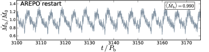
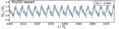
Figure 1.— Total binary accretion rate ${\dot{M\mkern 3.0mu}\mkern-3.0mu}{}_{\rm b}={\dot{M\mkern 3.0mu}\mkern-3.0mu}{}_{1}+{\dot{M\mkern 3.0mu}\mkern-3.0mu}{}_{2}$ for three steady-state tests over a period of 75.8 orbits (chosen to cover approximately 16 cycles of the accretion burst with frequency $\sim\tfrac{1}{5}\Omega_{\rm b}$). The same quasi-steady state is reached regardless of the different initial conditions (see Section 2.3.1).

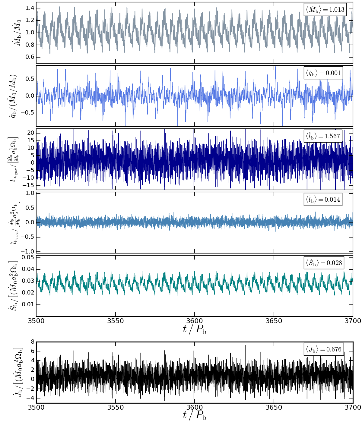
Figure 2.— The five different contributions to angular momentum transfer rate for an accreting circular binary and their combined effect ${\dot{J\mkern 3.0mu}\mkern-3.0mu}{}_{\rm b}$ according to Equations (2) and (4). From top to bottom ${\dot{M\mkern 3.0mu}\mkern-3.0mu}{}_{\rm b}$, $\dot{q}_{\rm b}$, $\dot{l}_{\rm b,grav}$, $\dot{l}_{\rm b,acc}$, $\dot{S}_{\rm b}\equiv\dot{S}_{1}+\dot{S}_{2}$ (see Section 2.2.1); and ${\dot{J\mkern 3.0mu}\mkern-3.0mu}{}_{\rm b}$. In steady state, $\langle{\dot{M\mkern 3.0mu}\mkern-3.0mu}{}_{\rm b}\rangle\approx{\dot{M\mkern 3.0mu}\mkern-3.0mu}{}_{0}$ and $\langle{\dot{J\mkern 3.0mu}\mkern-3.0mu}{}_{\rm b}\rangle\approx 0.676{\dot{M\mkern 3.0mu}\mkern-3.0mu}{}_{0}\Omega_{\rm b}a_{\rm b}^{2}$. Each time series is approximately stationary, with the time-averaged value indicated. The time sampling interval in each panel is $\approx 0.02P_{\rm b}$. The accretion eigenvalue in this case is $l_{0}\equiv\langle{\dot{J\mkern 3.0mu}\mkern-3.0mu}{}_{\rm b}\rangle/\langle{\dot{M\mkern 3.0mu}\mkern-3.0mu}{}_{\rm b}\rangle\approx 0.68\Omega_{\rm b}a_{\rm b}^{2}$ .

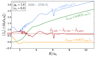
Figure 3.— Time-averaged angular momentum currents due to advection, viscosity and gravitational torques in the CBD for binary parameters $q_{\rm b}=1$ and $e_{\rm b}=0$ (see Section 2.2.2). The angular momentum currents are computed from the azimuthal integral of the angular momentum flux $F_{J}$ (Equation 16), and is time-averaged over a interval of $200\,P_{\rm b}$. The red curve is approximately constant, indicating quasi-steady-state. For reference, the net angular momentum change rate of the binary $\langle{\dot{J\mkern 3.0mu}\mkern-3.0mu}{}_{\rm b}\rangle=0.68{\dot{M\mkern 3.0mu}\mkern-3.0mu}{}_{0}\Omega_{\rm b}a_{\rm b}^{2}$ is overlaid as a straight red line. The “blip” at $R=6a_{\rm b}$ and fluctuations at $R\approx 2.5a_{\rm b}$ are artifacts of the mapping from the Voronoi cells onto a regular polar grid and their locations are sensitive to resolution in both the original simulation as in the remapped radial bins; such irregularities only appear in the $\dot{J}_{\rm adv}$ profile, which is always the noisiest of the different contributions to ${\dot{J\mkern 3.0mu}\mkern-3.0mu}{}_{\rm d}(R)$.

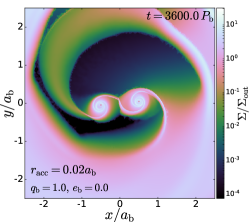
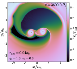
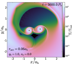
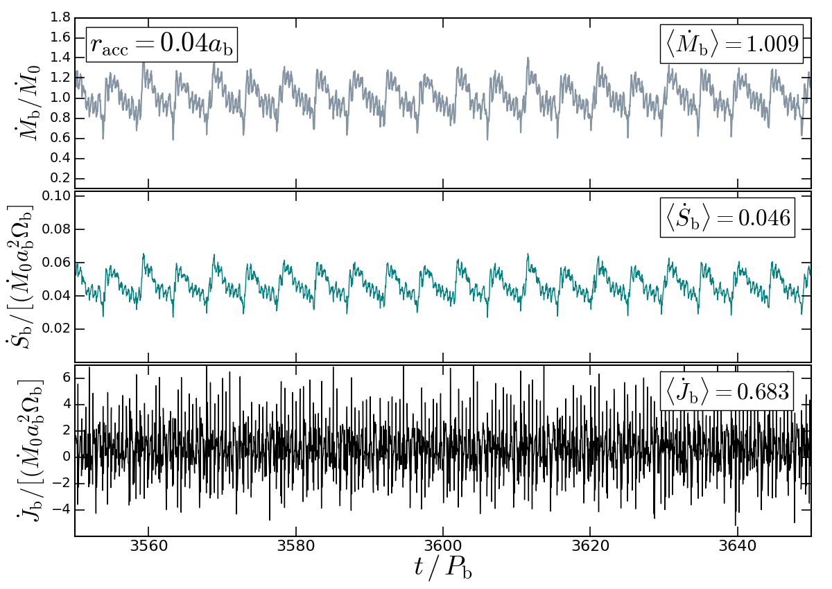
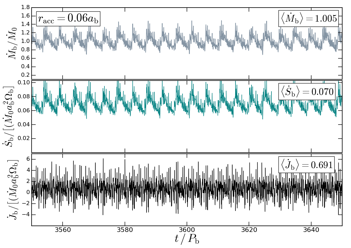
Figure 4.— Mass and angular momentum transfer for a circular binary for different values of the accretion (sink) radius $r_{\rm acc}$. The top panels depict the gas surface density rendered at $t=3600\,P_{\rm b}$ for $r_{\rm acc}=0.02a_{\rm b}$ (left), $r_{\rm acc}=0.04a_{\rm b}$ (middle) and $r_{\rm acc}=0.06a_{\rm b}$ (right). The bottom panels show the joint evolution of ${\dot{M\mkern 3.0mu}\mkern-3.0mu}{}_{\rm b}$, $\dot{S}_{\rm b}$ and ${\dot{J\mkern 3.0mu}\mkern-3.0mu}{}_{\rm b}$ over the interval $[3550\,P_{\rm b},3650\,P_{\rm b}]$ for $r_{\rm acc}=0.04a_{\rm b}$ (middle) and $r_{\rm acc}=0.06a_{\rm b}$ (right). Over the same time interval, all simulations exhibit highly consistent behavior in ${\dot{M\mkern 3.0mu}\mkern-3.0mu}{}_{\rm b}$ and ${\dot{J\mkern 3.0mu}\mkern-3.0mu}{}_{\rm b}$, with $\langle{\dot{J\mkern 3.0mu}\mkern-3.0mu}{}_{\rm b}\rangle/\langle{\dot{M\mkern 3.0mu}\mkern-3.0mu}{}_{\rm b}\rangle\approx 0.67-0.68$ (see Figure 2). The net spin torque $\langle{\dot{S\mkern 3.0mu}\mkern-3.0mu}{}_{\rm b}\rangle$ increases almost linearly with $r_{\rm acc}$, while $\langle{\dot{J\mkern 3.0mu}\mkern-3.0mu}{}_{\rm b}\rangle$ is not affected in a significant way.

Finally, we assume that radial transport is dominated by viscosity, and use

$$\begin{split}\upsilon_{R}^{\rm(visc)}(R)&=\frac{1}{R\Sigma}\frac{\partial}{\partial R}\left(\nu\Sigma R^{3}\frac{d\Omega}{dR}\right)\left[\frac{d}{dR}(R^{2}\Omega)\right]^{-1}\\ &=-3\alpha h_{0}^{2}\Omega_{\rm b}a_{\rm b}\left(\frac{R}{a_{\rm b}}\right)^{-1/2}\left[\frac{R}{\Sigma}\frac{d\Sigma}{dR}+1\right]\end{split}$$ (25)

as an estimate of the initial radial velocity, where we have taken $\Omega\approx\sqrt{\mathcal{G}M_{\rm b}/R}=\Omega_{\rm b}(R/a_{\rm b})^{-3/2}$. For our initial density profile (Equation 20), Equation (25) roughly matches the radial velocity profile of a steady-supply disk,

$$\upsilon_{R}^{\rm(steady)}=-\frac{\dot{M}_{0}}{2\pi R\Sigma}~{}~{},$$ (26)

for $R\gtrsim 15a_{\rm b}$. We have also experimented with setting $\upsilon_{R}=\upsilon_{R}^{\rm(steady)}$ as an initial condition and have found that a quasi-steady state can be reached faster. We stress that any axisymmetric initial condition is an inadequate representation of the gas dynamics for $R\lesssim 8a_{\rm b}$, and that the exact choice of the initial condition in this region is not critical to our results. It is of importance, however, that the simulation be evolved for a viscous time at a radius where the CBD can be considered axisymmetric and treated approximately as a conventional $\alpha$-disk. For an integration time of $t_{\rm int}=3000P_{\rm b}$, the disk is viscously relaxed out to a radius $R_{\rm rel}=a_{\rm b}[(9/2)\pi\alpha h_{0}^{2}(t_{\rm int}/P_{\rm b})]^{2/3}\approx 12a_{\rm b}$ (Rafikov, 2016; ML16). Therefore, outside this radius, the surface density will not have time to relax and will partially retain its initial configuration. It is then desirable that, already at $t=0$, the accretion rate profile roughly satisfies ${\dot{M\mkern 3.0mu}\mkern-3.0mu}{}(R)\approx{\dot{M\mkern 3.0mu}\mkern-3.0mu}{}_{0}$ for $R\gtrsim 20a_{\rm b}$; the initial condition (Equation 20) meets this requirement.

2.3.1 Steady-state tests

In order to test how close our initial condition is to a true steady state, we carry out three test integrations with $e_{\rm b}=0$: ($i$) we run an AREPO simulation with an open, diode-like boundary condition at $R=a_{\rm b}$ for $3000P_{\rm b}$ and then “release” the boundary to allow for direct accretion onto the binary, integrating for additional 500 orbits (see ML16); ($ii$) we allow for direct accretion onto the “stars” immediately at the start-up of the simulation and integrate for 500 orbits; ($iii$) we use the results of the PLUTO simulation from MML17 at $t=3000P_{\rm b}$, remapping it onto an AREPO grid and rescaling the units such that measured accretion rate at $R=15a_{\rm b}$ equals unity; then we proceed to evolve this setup integrating, as in cases ($i$) and ($ii$), for another 500 orbits. The accretion rates corresponding to these three tests are depicted in Figure 1. In all cases, after gas crosses the $R=a_{\rm b}$ boundary, only 5-20 orbits are needed for the CSDs to form. Another 20-30 orbits are needed for the binary to start accreting with an averaged rate equal to ${\dot{M\mkern 3.0mu}\mkern-3.0mu}{}_{0}$ to within a few percent. Eventually, ${\dot{M\mkern 3.0mu}\mkern-3.0mu}{}_{0}$ is matched to within $1\%$ in all cases, although this can take from 100 orbits (top panel) to 300 orbits (bottom panel). Overall, these three simulations are indistinguishable from each other, and we conclude that once quasi-steady-state is reached, the initial conditions become irrelevant.

From here on, we define quasi-steady-state as the state of the simulation for which the averaged accretion rate onto the binary $\langle{\dot{M\mkern 3.0mu}\mkern-3.0mu}{}_{\rm b}\rangle$ over an interval $T=100P_{\rm b}$ is equal to the mass supply rate ${\dot{M\mkern 3.0mu}\mkern-3.0mu}{}_{0}$ to within 2$\%$ and where the time averaged mass accretion profile in the CBD $\langle{\dot{M\mkern 3.0mu}\mkern-3.0mu}{}_{\rm d}\rangle(R)$ is also $\approx{\dot{M\mkern 3.0mu}\mkern-3.0mu}{}_{0}$ (i.e, flat to within an RMS tolerance of $5\%$). Unless stated otherwise, all simulations presented henceforth include a preliminary phase ($3000P_{\rm b}$) in which the disk is evolved using a diode boundary condition at $R_{\rm in}=a_{\rm b}(1+e_{\rm b})$. If a flat $\langle{\dot{M\mkern 3.0mu}\mkern-3.0mu}{}_{\rm d}\rangle$ profile is reached within that time period, the boundary is removed and the simulation is resumed in the self-consistent fashion described in the preceding paragraphs.

3. SIMULATION RESULTS

3.1. Results for a Circular Binary

Here, we explore the accretion behavior of a circular, equal-mass binary. We focus on the simulation output after 3500 binary orbits.

3.1.1 Angular momentum transfer

The simulation output is processed to produce time series for ${\dot{M\mkern 3.0mu}\mkern-3.0mu}{}_{\rm b}$ and $\dot{q}_{\rm b}$, the specific torques $dl_{\rm b}/dt|_{\rm grav}$ and $dl_{\rm b}/dt|_{\rm acc}$ and the spin change rate $\dot{S}_{\rm b}\equiv{\dot{S\mkern 3.0mu}\mkern-3.0mu}{}_{1}+{\dot{S\mkern 3.0mu}\mkern-3.0mu}{}_{2}$ (see Section 2.2.1). These quantities and the total ${\dot{J\mkern 3.0mu}\mkern-3.0mu}{}_{\rm b}$ are shown in Figure 2. for a time interval of $200P_{\rm b}$. We find that in quasi-steady-state, the time averaged ${\dot{J\mkern 3.0mu}\mkern-3.0mu}{}_{\rm b}$ is given by

$$\langle{\dot{J\mkern 3.0mu}\mkern-3.0mu}{}_{\rm b}\rangle\approx 0.676{\dot{M\mkern 3.0mu}\mkern-3.0mu}{}_{0}\Omega_{\rm b}a_{\rm b}^{2}~{}~{}.$$ (27)

Of the five different contributions to ${\dot{J\mkern 3.0mu}\mkern-3.0mu}{}_{\rm b}$, two quantities dominate over the rest: the mass change $\langle{\dot{M\mkern 3.0mu}\mkern-3.0mu}{}_{\rm b}\rangle\approx{\dot{M\mkern 3.0mu}\mkern-3.0mu}{}_{0}$ (first panel) and specific gravitational torque $\langle\dot{l}_{\rm b,grav}\rangle\approx 1.567({\dot{M\mkern 3.0mu}\mkern-3.0mu}{}_{0}/{M}_{\rm b})\Omega_{\rm b}a_{\rm b}^{2}$ (third panel).

The stationary nature of the ${\dot{M\mkern 3.0mu}\mkern-3.0mu}{}_{\rm b}$ and ${\dot{J\mkern 3.0mu}\mkern-3.0mu}{}_{\rm b}$ means that, in an averaged sense, a constant amount of angular momentum is transferred to the binary by the disk per unit accreted mass. This constant is the eigenvalue of the accretion flow (e.g. Paczynski, 1991; Popham & Narayan, 1991), i.e.,

$$\frac{\langle{\dot{J\mkern 3.0mu}\mkern-3.0mu}{}_{\rm b}\rangle}{\langle{\dot{M\mkern 3.0mu}\mkern-3.0mu}{}_{\rm b}\rangle}\equiv l_{0}~{}~{}.$$ (28)

Our result in Figure 2 implies

$$l_{0}\vphantom{\frac{1}{2}}\big{|}_{e_{\rm b}=0}\approx 0.68\Omega_{\rm b}a_{\rm b}^{2}~{}~{}.$$ (29)

The eigenvalue $l_{0}$ can also be obtained by computing $\langle{\dot{J\mkern 3.0mu}\mkern-3.0mu}{}_{\rm d}\rangle(R)$, the angular momentum current as a function of radius in the CBD (Equation 15). We compute ${\dot{J\mkern 3.0mu}\mkern-3.0mu}{}_{\rm d}(R)$ from the combination of ${\dot{J\mkern 3.0mu}\mkern-3.0mu}{}_{\rm d,adv}$, ${\dot{J\mkern 3.0mu}\mkern-3.0mu}{}_{\rm d,visc}$ and ${\dot{J\mkern 3.0mu}\mkern-3.0mu}{}_{\rm d,grav}$, in turn computed from the time averaged angular momentum flux maps $F_{J}$ as described in Section 2.2.2. We compute these angular momentum flux maps from simulation snapshots produced at a high output rate (15 snapshots per orbit) followed by time-averaging. Figure 3 shows the result. Importantly, we see that the net angular momentum current $\langle{\dot{J\mkern 3.0mu}\mkern-3.0mu}{}_{\rm d}\rangle(R)$ (dark red) is nearly flat for $R$ between $a_{\rm b}$ and $10a_{\rm b}$. Furthermore, $\langle{\dot{J\mkern 3.0mu}\mkern-3.0mu}{}_{\rm d}\rangle(R)$ is very close to $\langle{\dot{J\mkern 3.0mu}\mkern-3.0mu}{}_{\rm b}\rangle$. In other words, all of the angular momentum crossing the CBD is received by the binary. This provides convincing evidence that the exchange of mass and angular momentum between the CBD and the binary are in true quasi-steady-state, and that our computed eigenvalue (Equation 29) is reliable.

Dependence on sink radius

In our simulations, the ”stars” behave as sink particles. In most of our simulations, we adopt the “stellar radius” of $r_{\rm acc}=0.02a_{\rm b}$, but it is natural to evaluate how sensitive our results are to the choice of $r_{\rm acc}$. Recently, Tang et al. (2017) posited that the sign of the net angular momentum transfer rate $\langle{\dot{J\mkern 3.0mu}\mkern-3.0mu}{}_{\rm b}\rangle$ (note that Tang et al., 2017 only computed $\langle{\dot{L\mkern 3.0mu}\mkern-3.0mu}{}_{\rm b}\rangle$ and did not include spin torques) can depend critically on the way gas is drained from the computational domain by the stars (see Section 5.2.1 below). We test the influence of the accretion algorithm on our results by carrying out two additional simulations with $r_{\rm acc}=0.04a_{\rm b}$ and $r_{\rm acc}=0.06a_{\rm b}$ (the softening lengths are updated accordingly, but all other parameters remain unchanged). The results of this test are depicted in Figure 4, where we contrast the gas density field (to illustrate the effect of a larger sink radius) with the evolution of ${\dot{M\mkern 3.0mu}\mkern-3.0mu}{}_{\rm b}$, ${\dot{S\mkern 3.0mu}\mkern-3.0mu}{}_{\rm b}$ and ${\dot{J\mkern 3.0mu}\mkern-3.0mu}{}_{\rm b}$. The mean values $\langle{\dot{J\mkern 3.0mu}\mkern-3.0mu}{}_{\rm b}\rangle$ and $\langle{\dot{M\mkern 3.0mu}\mkern-3.0mu}{}_{\rm b}\rangle$ are robust against $r_{\rm acc}$, but $\langle{\dot{S\mkern 3.0mu}\mkern-3.0mu}{}_{\rm b}\rangle$ grows almost proportionally to $r_{\rm acc}$. Since $\langle{\dot{J\mkern 3.0mu}\mkern-3.0mu}{}_{\rm b}\rangle$ appears unmodified, the increase in $\langle{\dot{S\mkern 3.0mu}\mkern-3.0mu}{}_{\rm b}\rangle$ must be accompanied by a decrease in the torque $\mu_{\rm b}\langle\dot{l}_{\rm b,grav}\rangle$ (not shown). Indeed, over the interval $[3500,3700]P_{\rm b}$, the specific gravitational torque $\langle\dot{l}_{\rm b,grav}\rangle$ is $1.534({\dot{M\mkern 3.0mu}\mkern-3.0mu}{}_{0}/M_{\rm b})\Omega_{\rm b}a_{\rm b}^{2}$ when $r_{\rm acc}=0.04a_{\rm b}$ and $1.482({\dot{M\mkern 3.0mu}\mkern-3.0mu}{}_{0}/M_{\rm b})\Omega_{\rm b}a_{\rm b}^{2}$ when $r_{\rm acc}=0.06a_{\rm b}$, both smaller than the value of $1.567({\dot{M\mkern 3.0mu}\mkern-3.0mu}{}_{0}/M_{\rm b})\Omega_{\rm b}a_{\rm b}^{2}$ in our fiducial simulation (Fig. 2). The anisotropic accretion torque $\mu_{\rm b}\langle\dot{l}_{\rm b,acc}\rangle$ remains negligible in all cases. For all the values of $r_{\rm acc}$ explored, $\langle{\dot{S\mkern 3.0mu}\mkern-3.0mu}{}_{\rm b}\rangle$ is a small contribution to the total transfer of angular momentum to the binary $\langle{\dot{J\mkern 3.0mu}\mkern-3.0mu}{}_{\rm b}\rangle$. Presumably, a much larger value of $r_{\rm acc}$ than explored here – one that forbids the formation of CSDs – could make $\langle{\dot{S\mkern 3.0mu}\mkern-3.0mu}{}_{\rm b}\rangle$ an important contributor to $\langle{\dot{J\mkern 3.0mu}\mkern-3.0mu}{}_{\rm b}\rangle$, one that competes with $\mu_{\rm b}\dot{l}_{\rm b,grav}$, perhaps to the point of erasing the positive torque contribution of the CSDs, turning all the positive gain in orbital angular momentum into a growth in spin.

3.1.2 Understanding the Origin of the Positive Torque on the Binary: Spatial Distribution of Gravitational Torques

A major result of this paper (see Figs. 2-3), is that $\langle\dot{J}_{\rm b}\rangle\simeq\langle\dot{J}_{\rm d}\rangle>0$, i.e., an accreting binary gains angular momentum from a steady-supply disk. From Figure 2, we see that a major contribution to $\langle\dot{J}_{\rm b}\rangle$ comes from the total gravitational torque $\mu_{\rm b}\langle\dot{l}_{\rm b,grav}\rangle$ (third panel), which is positive, in apparent contradiction with what one might expect from theoretical work (Goldreich & Tremaine, 1980; Artymowicz & Lubow, 1994; Lubow & Artymowicz, 1996), since the linear theory of Lindblad torques of Goldreich & Tremaine (1979) predicts that an outer disk exerts negative torques on the inner binary. Note that our result for the angular momentum current ${\dot{J\mkern 3.0mu}\mkern-3.0mu}{}_{\rm d,grav}$ in the CBD (Figure 3, yellow curve) is indeed consistent with this theoretical expectation. However, a self-consistent calculation of $\langle\dot{J}_{\rm b}\rangle$ needs to include the entire distribution of gas, and not only that of the CBD.

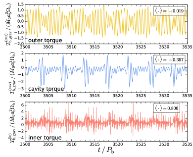
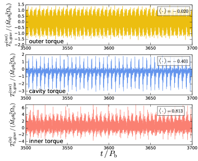
Figure 5.— Gravitational torques dissected according to distance $R$ from the binary barycenter (Section 2.3) as a function of time, covering the time interval between 3500 and 3535 $P_{\rm b}$ (left panels) and between 3500 to 3700 $P_{\rm b}$ (right panels). The outer torque (yellow, top panels) corresponds to the torque exerted by gas cells located at $R>R_{\rm cav})$ (see Equation 22); the cavity torque (blue, middle panels) corresponds to the total torque exerted by cells with radii $a_{\rm b}<R<R_{\rm cav}$; the inner torque (red, bottom panels) corresponds to cells with $R<a_{\rm b}$. The mean values of these torques are indicated in each panel. Both the cavity and outer torques are negative, collectively amounting to $\approx-0.42{\dot{M\mkern 3.0mu}\mkern-3.0mu}{}_{0}\Omega_{\rm b}a_{\rm b}^{2}$, in agreement with ${\dot{J\mkern 3.0mu}\mkern-3.0mu}{}_{\rm d,grav}$ at $R=a_{\rm b}$ (Figure 3). A net negative gravitational torque due to gas outside $R=a_{\rm b}$ is in agreement with theoretical expectations and past numerical work. The net positive sign of $\langle T_{\rm b,grav}\rangle$ is due to the large inner torque $\langle T_{\rm b,grav}^{\rm(in)}\rangle$. Over 200 orbits (right panels), the net gravitational torque $\langle T_{\rm b,grav}\rangle=0.392{\dot{M\mkern 3.0mu}\mkern-3.0mu}{}_{0}\Omega_{\rm b}a_{\rm b}^{2}$ is equal to the specific torque $\langle\dot{l}_{\rm b,grav}\rangle=1.567({\dot{M\mkern 3.0mu}\mkern-3.0mu}{}_{0}/M_{\rm b})\Omega_{\rm b}a_{\rm b}^{2}$ (third panel of Fig. 2) multiplied by the reduced mass $\mu_{\rm b}=M_{\rm b}/4$. The inner torque exhibits rapid variability on time-scales $\sim P_{\rm b}/100$ and its mean value, when properly measured, can double in magnitude the negative torque due to the outer/cavity gas. Comparison between the left and right panels shows that a few tens of orbits are sufficient to capture the basic stationary behavior of these torque time series.

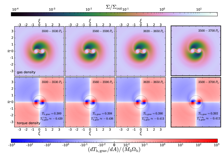
Figure 6.— Stacked (averaged) maps of the mass density $\Sigma$ (top panels) and the gravitational torque density $dT_{\rm b,grav}/d{\rm A}$ (bottom panels) for accretion onto a circular binary. From left to right, the stacked maps for three different time windows of length $30P_{\rm b}$ (corresponding to 450 snapshots) are shown: 3500 to 3530 orbits, 3560 to 3590 orbits and 3620 to 3650 orbits. The differences between these maps are virtually unnoticeable, suggesting that $\simeq 30$ orbits is sufficient integration time to capture the essential behavior of the accreting binary. The integrated torque maps over area outside $R=a_{\rm b}$ is $T_{\rm b}^{>a_{\rm b}}\simeq-0.41{\dot{M\mkern 3.0mu}\mkern-3.0mu}{}_{0}\Omega_{\rm b}a_{\rm b}^{2}$, which is roughly consistent over time. The last column shows the stacking of 3000 reconstructed maps over 200 binary orbits; again, the overall morphology appears to be unchanged over longer timescales.

Figure 5 depicts the dissection of the total gravitational torque $T_{\rm b,grav}=\mu_{\rm b}\dot{l}_{\rm b,grav}$ into 3 components (from top to bottom): (i) the outer disk torque $T_{\rm b,grav}^{\rm(out)}$ ($R>R_{\rm cav}$; with $R_{\rm cav}$ as defined in Equation 22), (ii) the “cavity+streams” torque $T_{\rm b,grav}^{\rm(cav)}$ ($a_{\rm b}\leq R\leq R_{\rm cav}$); and (iii) the “inner” torque $T_{\rm b,grav}^{\rm(in)}$ ($R<a_{\rm b}$). The short-term evolution of these torques is depicted on the left panels of the figure, and the long-term evolution is shown on the right. On average, the sum of these 3 different torques must equal $\langle T_{\rm b,grav}\rangle=\mu_{\rm b}\langle\dot{l}_{\rm b,grav}\rangle=0.392{\dot{M\mkern 3.0mu}\mkern-3.0mu}{}_{0}a_{\rm b}^{2}\Omega_{\rm b}$.

From the torque dissection, we confirm that the gravitational torque acting on the binary due to the material outside $R=a_{\rm b}$ is indeed negative, but that the material inside $R=a_{\rm b}$ exerts a positive torque that nearly doubles in magnitude the negative outer torque. We also find that the oscillation amplitudes of these three torque contributions can be much larger than their mean values. In order to capture both the rapid sign changes in $T_{\rm b,grav}^{\rm(out)}$, $T_{\rm b,grav}^{\rm(cav)}$ and $T_{\rm b,grav}^{\rm(in)}$ as well as their long-term averages, a fine sampling in time as well as a long-term integration are required. We find that a sample rate of 15 snapshots per binary orbit captures $T_{\rm b,grav}^{\rm(out)}$ and $T_{\rm b,grav}^{\rm(cav)}$ adequately since they vary on timescales of $\sim P_{\rm b}$; however, since $T_{\rm b,grav}^{\rm(in)}$ can vary on timescales comparable to the orbital period within the CSDs, we need a sampling rate of $\sim 100$ snapshots per orbit to capture such rapid variability. This rapid variability is difficult to capture from post-processing analysis of simulation snapshots, but is automatically accounted for by the strategy described in Section 2.2.1.

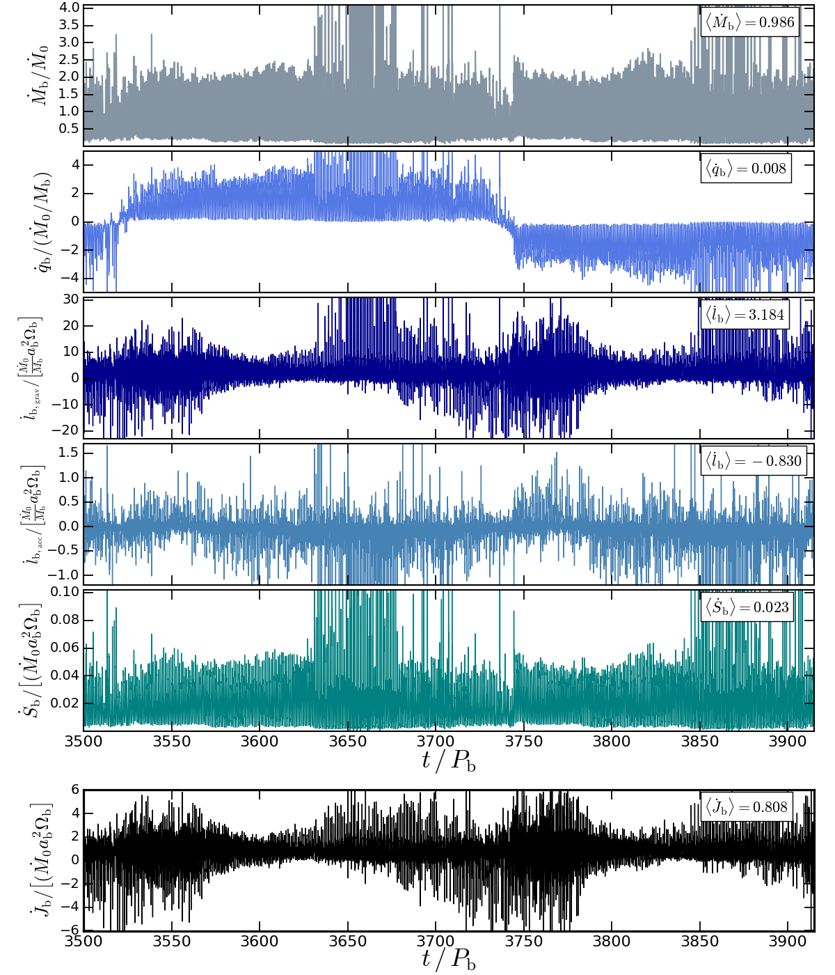
Figure 7.— The five different contributions to angular momentum transfer rate and its combined effect ${\dot{J\mkern 3.0mu}\mkern-3.0mu}{}_{\rm b}$ (Equations 2 and 4), for an eccentric ($e_{\rm b}=0.6$) binary. Panels are the same as in Figure 2, with the only difference being the time axis, which covers 415 binary orbits (as opposed to the 200 of the $e_{\rm b}=0$ case). The extent of the time axis is chosen to roughly match the alternation period in mass accretion (see change in the sign of $\dot{q}_{\rm b}$ in second panel from top). The accretion eigenvalue in this case is $l_{0}\approx 0.81\Omega_{\rm b}a_{\rm b}^{2}$. We have also explored the evolution of these same quantities for the time interval $[3985\,P_{\rm b},4400\,P_{\rm b}]$, confirming that the $\langle{\dot{M\mkern 3.0mu}\mkern-3.0mu}{}_{\rm b}\rangle$ and $\langle{\dot{J\mkern 3.0mu}\mkern-3.0mu}{}_{\rm b}\rangle$ are unchanged.

The contribution of the cavity region to the gravitational torque can be better understood if we explore the spatial distribution of the torque in two dimensions. For this, we construct gravitational torque density maps. Evidently, since $-\mathbf{T}_{\rm b,grav}=\mathbf{T}_{\rm d,grav}$ (the torque exerted on the disk by the binary), the torque per unit area can be computed directly from the cell-centered values of density and gravitational acceleration:

$$\begin{split}\frac{d\mathbf{T}_{\rm b,grav}}{d{\rm A}}(\mathbf{r})=-\frac{d\mathbf{T}_{\rm d,grav}}{d{\rm A}}(\mathbf{r})&=\Sigma(\mathbf{r})\mathbf{r}\times\nabla\Phi_{\rm b}(\mathbf{r})\\ &\approx-\Sigma_{k}\mathbf{r}_{k}\times\mathbf{a}_{k}~{}~{},\end{split}$$ (30)

where $\mathbf{a}_{k}$ is the gravitational acceleration of the gas and the subscript $k$ denotes evaluation at the center of a cell.

To explore the long-term effect of the nonaxisymmetric features in the circumbinary gas, we can take time averages of both the density and torque density fields. This is shown in Figure 6, where we have stacked the density field $\Sigma$ and the torque per unit area (Equation 30) (15 snapshots per orbit) rotated by an angle that matches the rotation of the binary. The coordinates axes in this figure are thus $\xi$ and $\eta$, related to the original coordinates by the area-preserving transformation $x=a_{\rm b}(\xi\cos f_{\rm b}-\eta\sin f_{\rm b})$ and $y=a_{\rm b}(\xi\sin f_{\rm b}+\eta\cos f_{\rm b})$ . We carry out this average over intervals of $\sim 30$ orbits in duration, at different times in the simulation. In addition, we perform the average over 200 orbits (rightmost panels of Figure 6). All the averaging sets produce essentially the same result, implying that most of the variability takes place on timescales shorter than 30 orbits. Figure 6 reveals that the streamers are the dominant nonaxisymmetric feature that persists in time. From the torque density maps (bottom panels) it can be seen that different portions of the gas can “torque up” (regions in red) or “torque down” (regions in blue) the binary, but only the persistent nonaxisymmetric features contribute to the non-zero net torque.

3.2. Results for an Eccentric Binary

We repeat the numerical simulations of Section 3.1, this time for binary eccentricity $e_{\rm b}=0.6$. Several differences between these two calculations are expected. First, the lump that modulates the accretion every $\sim 5$ binary orbits when $e_{\rm b}=0$ (e.g., MacFadyen & Milosavljević, 2008; Shi et al., 2012; ML16; MML17) is no longer present (ML16; for these values of $\alpha$ and $h_{0}$, MML17 find that the lump disappears at $e_{\rm b}\gtrsim 0.05$). Second, accretion will be preferential and alternating (Dunhill et al., 2015; ML16), i.e., the primary and secondary will alternate over precessional timescales which one receives most of the mass. Third, the gas distribution and kinematics in the region $R\lesssim a_{\rm b}$ differ significantly from the circular case (material enters and leaves this region in a periodic fashion, see Fig. 2 of ML16), affecting the amount of torque that this region can provide to counterbalance the torque from the CBD.

3.2.1 Angular momentum transfer

In Figure 7 we show the total angular momentum transfer rate ${\dot{J\mkern 3.0mu}\mkern-3.0mu}{}_{\rm b}$ and its various contributions for a $q_{\rm b}=1$, $e_{\rm b}=0.6$ binary. As expected, we find that ${\dot{M\mkern 3.0mu}\mkern-3.0mu}{}_{\rm b}$ is no longer modulated at a frequency of $\sim\tfrac{1}{5}\Omega_{\rm b}$, but at the dominant frequency $\sim\Omega_{\rm b}$ (ML16). There are variations over much longer timescales: the mass ratio change $\dot{q}_{\rm b}$ flips signs every $\sim 415\,P_{\rm b}$. The gravitational specific torque $\dot{l}_{\rm b,grav}$ is again positive, and larger than in the circular case. The contribution of the anisotropic accretion torque $\mu_{\rm b}\langle\dot{l}_{\rm b,acc}\rangle\approx-0.21{\dot{M\mkern 3.0mu}\mkern-3.0mu}{}_{0}\Omega_{\rm b}a_{\rm b}^{2}$ is no longer negligible. As in the circular case, the contribution of the spin torque $\langle{\dot{S\mkern 3.0mu}\mkern-3.0mu}{}_{\rm b}\rangle$ to the total torque $\langle{\dot{J\mkern 3.0mu}\mkern-3.0mu}{}_{\rm b}\rangle$ is small ($\sim 2\%$).

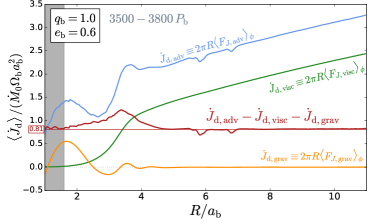
Figure 8.— Similar to Figure 3, except for an eccentric binary ($e_{\rm b}=0.6$). The thin red line indicates the eigenvalue $l_{0}=0.81a_{\rm b}^{2}\Omega_{\rm b}$ (Equation 31) obtained from the evolution of the accreting eccentric binary (Figure 7). The gray region represents the portion of the computational domain left out by the diode-like boundary at $R=a_{\rm b}(1+e_{\rm b})$ in the PLUTO simulations of MML17 and is depicted here only for reference. The $30\%$ discrepancy at $R\approx 3a_{\rm b}$ is likely due to a combination of insufficiently dense sampling in time and the incomplete coverage of apsidal precession period of the disk, in addition to the intrinsic difficulties of estimating the advective flux of angular momentum from reconstructed primitive variables.

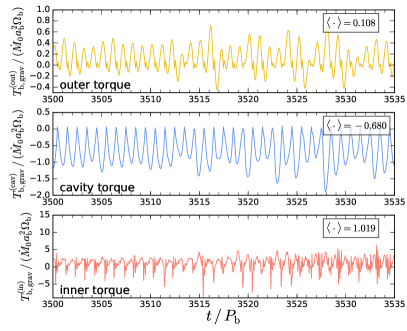
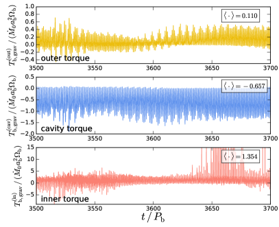
Figure 9.— Similar to Figure 5, this time for an eccentric binary ($e_{\rm b}=0.6$). The total gravitational torque is dissected into an outer component (yellow, top panels) for $R>R_{\rm cav}$, a cavity components (blue, middle panel) for $a_{\rm b}(1+e_{\rm b})<R\leq R_{\rm cav}$, and an inner component (red, bottom panels) for $R\leq a_{\rm b}(1+e_{\rm b})$. The gravitational torque due to gas outside the boundary $R=a_{\rm b}(1+e_{\rm b})$ is negative, but smaller in magnitude than the positive torque due to gas inside that boundary. Over 200 orbits (right panels), the net gravitational torque $\langle T_{\rm b,grav}\rangle=0.807{\dot{M\mkern 3.0mu}\mkern-3.0mu}{}_{0}\Omega_{\rm b}a_{\rm b}^{2}$ is equal to the specific torque $\langle\dot{l}_{\rm b,grav}\rangle=3.229({\dot{M\mkern 3.0mu}\mkern-3.0mu}{}_{0}/M_{\rm b})\Omega_{\rm b}a_{\rm b}^{2}$ (extracting the interval $[3500,3700]P_{\rm b}$ from the third panel of Fig. 7) and multiplied by the reduced mass $\mu_{\rm b}=M_{\rm b}/4$.

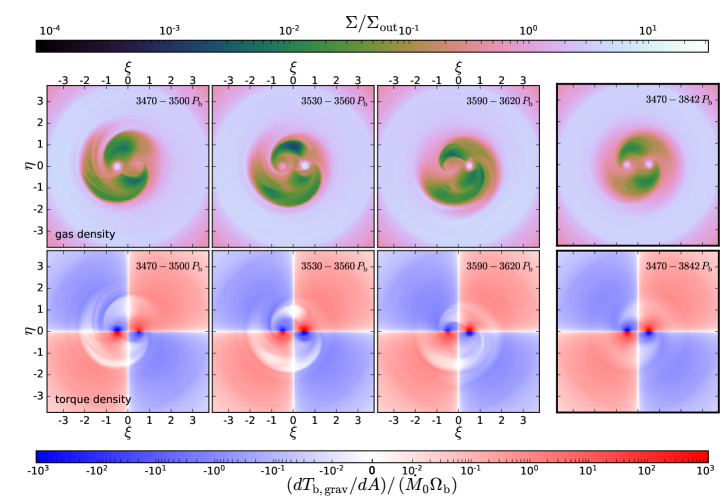
Figure 10.— Stacking of mass density and torque density maps, similar to Figure 6, this time for a binary with $e_{\rm b}=0.6$. Stacking is carried out in the rotating-pulsating coordinate frame of the eccentric binary (see text); in this frame, the primary and secondary remain along the horizontal axis, with fixed coordinates $\xi=-0.5$ and $\xi=0.5$ respectively. From left to right, we show three time windows of length $30\,P_{\rm b}$: 3470 to 3500 orbits, 3530 to 3560 orbits, and 3500 to 3620 orbits. In contrast to Figure 6, these stacked frames are evidently not exhibiting stationarity. Most notable is the asymmetry in the surface density of the CSDs: in the first map, the disk around the primary is mass loaded, while the one around the secondary is barely visible; in the second map, a transition has taken place, where the secondary disk contains more mass; in the third map, the secondary disk is loaded, while the cicum-primary disk is empty. This transition is consistent with what is observed in the time series of ${\dot{M\mkern 3.0mu}\mkern-3.0mu}{}_{1}$ and ${\dot{M\mkern 3.0mu}\mkern-3.0mu}{}_{2}$ (ML16) and in the long-term behavior of $\dot{q}_{\rm b}$ in Figure 7. This long-term variability is apparent in the change of integrated torque outside the binary $T_{\rm b,grav}^{>1.6a_{\rm b}}$. The last column on the right depicts the stacking of 4935 maps of $\Sigma$ and $dT_{\rm b,grav}/dA$ over 372 binary orbits; most of the variability is removed, and the surface density map shows a great degree of symmetry, with both CSDs containing similar amounts of mass.

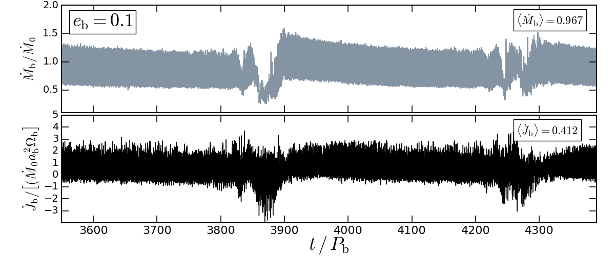
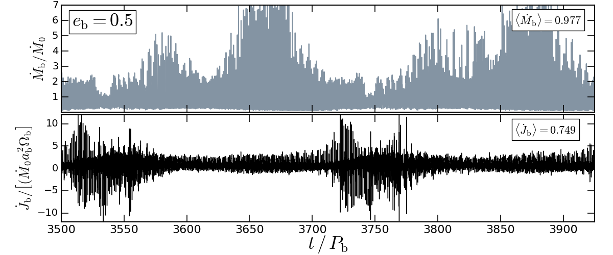
Figure 11.— Similar to Figs. 2 and 7, but for binaries with $e_{\rm b}=0.1$ and $e_{\rm b}=0.5$, and only showing ${\dot{M\mkern 3.0mu}\mkern-3.0mu}{}_{\rm b}$ (gray) and ${\dot{J\mkern 3.0mu}\mkern-3.0mu}{}_{\rm b}$ (black). The accretion eigenvalue is $l_{0}\approx 0.43\Omega_{\rm b}a_{\rm b}^{2}$ for $e_{\rm b}=0.1$ and $l_{0}\approx 0.78\Omega_{\rm b}a_{\rm b}^{2}$ for $e_{\rm b}=0.5$.

As in Section 3.1, we can compute the accretion eigenvalue $l_{0}$ directly from the result shown in Figure 7, giving

$$l_{0}\vphantom{\frac{1}{2}}\big{|}_{e_{\rm b}=0.6}\approx 0.81\Omega_{\rm b}a_{\rm b}^{2}~{}~{}.$$ (31)

We also compute the net angular momentum current in the CBD ${\dot{J\mkern 3.0mu}\mkern-3.0mu}{}_{\rm d}(R)$ (Section 2.2.2) averaged over 300 orbits, as shown in Figure 8. We see that $\langle{\dot{J\mkern 3.0mu}\mkern-3.0mu}{}_{\rm d}\rangle(R)$ is approximately constant (independent of $R$) and equal to $\langle{\dot{J\mkern 3.0mu}\mkern-3.0mu}{}_{\rm b}\rangle$ , indicating that the global angular momentum balance is achieved. In this case, the match between $\langle{\dot{J\mkern 3.0mu}\mkern-3.0mu}{}_{\rm d}\rangle/{\dot{M\mkern 3.0mu}\mkern-3.0mu}{}_{0}$ and $l_{0}=0.81\Omega_{\rm b}a_{\rm b}^{2}$ is remarkable for $R>4a_{\rm b}$ and $R<2a_{\rm b}$.

3.2.2 Spatial Distribution of Gravitational Torques

As in the case of the circular binary, the eccentric binary gains angular momentum, which, as before, is largely a result of the positive net gravitational torque $\langle T_{\rm b,grav}\rangle=\mu_{\rm b}\langle\dot{l}_{\rm b,grav}\rangle\approx 0.796{\dot{M\mkern 3.0mu}\mkern-3.0mu}{}_{0}\Omega_{\rm b}a_{\rm b}^{2}$. As before, we study the spatial distribution of gravitational torques in the simulation by splitting $T_{\rm b,grav}$ into three components: $T_{\rm b,grav}^{\rm(out)}$, $T_{\rm b,grav}^{\rm(cav)}$ and $T_{\rm b,grav}^{\rm(in)}$ (Figure 9). We see a similar behavior to that of a circular binary (Figure 5): the sum $T_{\rm b,grav}^{\rm(out)}+T_{\rm b,grav}^{\rm(cav)}$ is negative (dominated by $T_{\rm b,grav}^{\rm(cav)}$) while the positive sign of the total torque $\langle T_{\rm b,grav}\rangle$ is entirely due to the positive sign of $T_{\rm b,grav}^{\rm(in)}$. The torque time series shown in Figure 9 exhibit some degree of regularity, but they differ from the nearly exact periodicity seen in Figure 5. As noted above, the accretion flow onto eccentric binaries is modulated over long secular timescales, and it is not surprising that a few tens of orbits cannot capture the entire range of time variability.

The fact that tens of orbits is too short a time span to reveal the underlying stationary behavior the accretion flow can be illustrated by repeating the map-stacking analysis for the $e_{\rm b}=0.6$ case (see Figure 10; cf. Figure 6). The stacking of these images is trickier than in the circular case: in order for the two “stars” to line-up at all snapshots, we need to introduce a rotating-pulsating coordinate system, a transformation that is well known in the study of the elliptical restricted three-body problem (ER3BP; e.g., Nechvíle, 1926; Kopal & Lyttleton, 1963; Szebehely & Giacaglia, 1964; Szebehely, 1967; Musielak & Quarles, 2014). The scaled, rotated coordinates $\xi$ and $\eta$ are related to the barycentric coordinates $x$ and $y$ by: $x=r_{\rm b}(\xi\cos f_{\rm b}-\eta\sin f_{\rm b})$ and $y=r_{\rm b}(\xi\sin f_{\rm b}+\eta\cos f_{\rm b})$, where $r_{\rm b}=a_{\rm b}(1-e^{2}_{\rm b})/(1+e_{\rm b}\cos f_{\rm b})$ and $f_{\rm b}$ is the true anomaly of the binary. This transformation is not area preserving, thus scalars must be transformed by multiplying by the Jacobian of the transformation ($=r_{\rm b}^{2}$). In Figure 10 (top row, left to right), we show $\Sigma$ stacked over the time intervals $[3470\,P_{\rm b},3500\,P_{\rm b}]$, $[3530\,P_{\rm b},3560\,P_{\rm b}]$, $[3590\,P_{\rm b},3620\,P_{\rm b}]$ and $[3470\,P_{\rm b},3799\,P_{\rm b}]$. These reveal a striking, inherent property of accretion onto eccentric binaries: the “loading” of the CSDs alternates in time, i.e., the gas surface density is higher in one CSD than in the other. This disk loading can be directly tied to the sign of $\dot{q}_{\rm b}$ in Fig 7. When we average over 370$P_{\rm b}$ – almost the entire precessional period identified from the time series of $\dot{q}_{\rm b}$ – we see that most of the asymmetries disappear (the last column of Figure 10), and that the distribution of gas starts to resemble that of the circular case (Figure 6). Note how the shape of the cavity also changes as preferential accretion switches recipients, as it is expected if alternation is caused by the precession of the cavity edge.

We use this rotating system to study the spatial distribution of torques, albeit only in a qualitative manner (Figure 10). Some similarities can be found with the analogous plot for the circular case (Figure 6, bottom row), although the spatial distribution of torques in the eccentric case is more diffuse and variable. A direct comparison to the spatial torque dissection of Figure 9 is not possible, since the barycentric radial coordinate $R$ changes from snapshot to snapshot in the rotating-pulsating coordinate system.

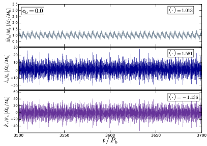
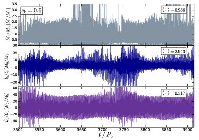
Figure 12.— Evolution of the rate of change in mass ${\dot{M\mkern 3.0mu}\mkern-3.0mu}{}_{\rm b}/{M}_{\rm b}$ (top), specific angular momentum $\dot{l}_{\rm b}/{l}_{\rm b}$ (middle) and specific energy ${\dot{\mathcal{E}\mkern 3.0mu}\mkern-3.0mu}{}_{\rm b}/\mathcal{E}_{\rm b}$ (bottom) for the $e_{\rm b}=0$ binary (left panels) and the $e_{\rm b}=0.6$ binary (right panels). These quantities determine the rate of change of the orbital elements $\dot{e}_{\rm b}$ and $\dot{a}_{\rm b}$ via Eqs. (34) and (35).

3.3. Other Values of Binary Eccentricity

We have repeated the experiments of Sections 3.1 and 3.2 for other values of the binary eccentricity. Figure 11 shows the results for a low eccentricity binary ($e_{\rm b}=0.1$, top) and an intermediate eccentricity binary ($e_{\rm b}=0.5$, bottom). In both cases, the circumbinary cavity lacks the accretion lump (MML17), and accretion exhibits long-term alternation. As in Figure 7, the time interval in the $x$-axis is chosen to cover and entire precessional period, estimated as the time it takes for $\dot{q}_{\rm b}$ to change sign twice. This period is measured to be $\sim 800P_{\rm b}$ for $e_{\rm b}=0.1$ and $\sim 400P_{\rm b}$ for $e_{\rm b}=0.5$. Note that this alternation period does not exactly match the apsidal precession period of test particles at the location of the cavity edge (e.g., Thun et al., 2017), since the latter scales with cavity size and eccentricity as $(R_{\rm cav}/a_{\rm b})^{7/2}(1+\tfrac{3}{2}e_{\rm b}^{2})^{-1}$ (Eq. 7 in ML16), which, if we take Equation (22) at face value, implies that the precession period scales as $e_{\rm b}^{7/2}$. However, the precession rate of the inner CBD can be coherent out to $R\sim 20a_{\rm b}$ (e.g., Fig. 9 in MML17), and then it does not need to be set by the precession rate at $R_{\rm cav}$, but rather by some mean rate over that range of radii.

Table 1Summary of simulation results

$e_{\rm b}$	$r_{\rm acc}$	$\langle{\dot{J\mkern 3.0mu}\mkern-3.0mu}{}_{\rm b}\rangle/\langle{\dot{M\mkern 3.0mu}\mkern-3.0mu}{}_{\rm b}\rangle$	$\langle{\dot{S\mkern 3.0mu}\mkern-3.0mu}{}_{\rm b}\rangle/\langle{\dot{M\mkern 3.0mu}\mkern-3.0mu}{}_{\rm b}\rangle$	$\langle\dot{a}_{\rm b}\rangle$	$\langle\dot{e}_{\rm b}\rangle$	$T$
	$[a_{\rm b}]$	$[\Omega_{\rm b}a_{\rm b}^{2}]$	$[\Omega_{\rm b}a_{\rm b}^{2}]$	$[a_{\rm b}{\dot{M\mkern 3.0mu}\mkern-3.0mu}{}_{0}/M_{\rm b}]$	$[{\dot{M\mkern 3.0mu}\mkern-3.0mu}{}_{0}/M_{\rm b}]$	$[P_{\rm b}]$
0	0.02	0.68	0.028	2.15	-0.004	200
	0.04	0.68	0.046	2.05	-0.008	200
	0.06	0.69	0.07	2.00	-0.025	200
0.1	0.02	0.43	0.023	0.75	2.42	800
0.5	0.02	0.78	0.025	0.95	-0.20	415
0.6	0.02	0.81	0.023	0.47	-2.34	415

Note. — Simulation parameters are the binary eccentricity $e_{\rm b}$ and the accretion radius $r_{\rm acc}$. The results include the long-term averages of the binary’s angular momentum change rate $\langle{\dot{J\mkern 3.0mu}\mkern-3.0mu}{}_{\rm b}\rangle$, the spin torque $\langle{\dot{S\mkern 3.0mu}\mkern-3.0mu}{}_{\rm b}\rangle=\langle{\dot{S\mkern 3.0mu}\mkern-3.0mu}{}_{1}\rangle+\langle{\dot{S\mkern 3.0mu}\mkern-3.0mu}{}_{2}\rangle$, the semimajor axis change rate $\langle\dot{a}_{\rm b}\rangle$ and the eccentricity change rate $\langle\dot{e}_{\rm b}\rangle$. The averaged mass accretion rate onto the binary $\langle{\dot{M\mkern 3.0mu}\mkern-3.0mu}{}_{\rm b}\rangle$ equals to the mass supply rate ${\dot{M\mkern 3.0mu}\mkern-3.0mu}{}_{0}$. The binary’s orbital angular momentum change rate is $\langle{\dot{L\mkern 3.0mu}\mkern-3.0mu}{}_{\rm b}\rangle=\langle{\dot{J\mkern 3.0mu}\mkern-3.0mu}{}_{\rm b}\rangle-\langle{\dot{S\mkern 3.0mu}\mkern-3.0mu}{}_{\rm b}\rangle$. Averages are taken over a time interval $T$(chosen to cover one full cycle in alternating accretion).

The main conclusion drawn from Figure 11 is that, provided that steady-state is reached, the net transfer of angular momentum to the binary $\langle{\dot{J\mkern 3.0mu}\mkern-3.0mu}{}_{\rm b}\rangle$ is positive for various values of $e_{\rm b}$. As in the circular binary case, to obtain a reliable measurement of $\langle{\dot{J\mkern 3.0mu}\mkern-3.0mu}{}_{\rm b}\rangle$, it is important to capture accurately the gravitational torques from the CSDs, which are positive and can counterbalance the negative torques due to the CBD.

We summarize the results of our simulations in Table 1. In all cases explored – a circular binary with three values of $r_{\rm acc}$ and three eccentric binaries – the binary experiences a net gain in angular momentum. There are multiple consequences of having $\langle{\dot{J\mkern 3.0mu}\mkern-3.0mu}{}_{\rm b}\rangle>0$. In particular, we are interested in translating $\langle{\dot{M\mkern 3.0mu}\mkern-3.0mu}{}_{\rm b}\rangle$ and $\langle{\dot{J\mkern 3.0mu}\mkern-3.0mu}{}_{\rm b}\rangle$ into secular changes in the orbital elements of the binary. We explore this in the next section.

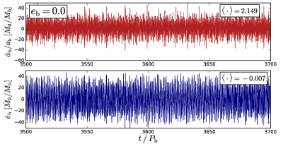
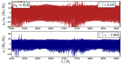
Figure 13.— Binary semimajor axis change rate (top, red) and the binary eccentricity change rate (bottom, blue) for circular and eccentric binaries according to Eqs. (36) and (37) and the simulation results of Sections 3.1 and 3.2. Left panels ($e_{\rm b}=0$): the mean values $\langle\dot{a}_{\rm b}\rangle\approx 2.15a_{\rm b}{\dot{M\mkern 3.0mu}\mkern-3.0mu}{}_{0}/M_{\rm b}$ and $\langle\dot{e}_{\rm b}\rangle\approx 0$, indicate that a circular binary tends to remain circular, but that its semimajor axis grows in time. Right panels ($e_{\rm b}=0.6$): the binary expands and circularizes ($\langle\dot{a}_{\rm b}\rangle\approx 0.38a_{\rm b}{\dot{M\mkern 3.0mu}\mkern-3.0mu}{}_{0}/M_{\rm b}$ and $\langle\dot{e}_{\rm b}\rangle\approx-2.34{\dot{M\mkern 3.0mu}\mkern-3.0mu}{}_{0}/M_{\rm b}$). Both circular and eccentric binaries exhibit similar RMS variability in $\dot{a}_{\rm b}$ and $\dot{e}_{\rm b}$, except during the the irregular bursts that take place each time $\dot{q}_{\rm b}$ switches signs in the eccentric case (at $t/P_{\rm b}\sim 3520$ and $\sim 3740$).

4. Orbital Evolution of Accreting Binaries

For a circular, equal-mass binary, the time-averaged rates $\langle{\dot{M\mkern 3.0mu}\mkern-3.0mu}{}_{\rm b}\rangle$ and $\langle{\dot{L\mkern 3.0mu}\mkern-3.0mu}{}_{\rm b}\rangle\simeq\langle{\dot{J\mkern 3.0mu}\mkern-3.0mu}{}_{\rm b}\rangle$ completely determine the secular semi-major axis evolution $\langle\dot{a}_{\rm b}\rangle$ of the binary (assuming that the binary remains circular). For an eccentric binary, more information is needed. The orbital evolution of variable mass binaries has long been studied (e.g. Brown, 1925; Jeans, 1925; Hadjidemetriou, 1963; Verhulst, 1972; Veras et al., 2011). Hadjidemetriou (1963) derived the evolution equation for the binary orbital elements due to time-varying mass loss by introducing a fictitious force. Here, we give a much simpler derivation of $\dot{a}_{\rm b}$ and $\dot{e}_{\rm b}$ for a mass losing/gaining binary using energy and angular momentum conservation. We employ two methods to evaluate $\langle\dot{a}_{\rm b}\rangle$ and $\langle\dot{e}_{\rm b}\rangle$ using our simulation output.

Consider the specific angular momentum $\mathbf{l}_{\rm b}=\mathbf{r}_{\rm b}\times\dot{\mathbf{r}}_{\rm b}$ and specific energy $\mathcal{E}_{\rm b}=\tfrac{1}{2}\dot{\mathbf{r}}_{\rm b}^{2}-\mathcal{G}M_{\rm b}/r_{\rm b}$ of the binary. The equation of motion is ${d\dot{\mathbf{r}}_{\rm b}}/{dt}=-({\mathcal{G}{M}_{\rm b}}/{r_{\rm b}^{3}}){\mathbf{r}}_{\rm b}+\mathbf{f}_{\rm ext}$ where $\mathbf{f}_{\rm ext}\equiv\mathbf{f}_{\rm ext,1}-\mathbf{f}_{\rm ext,2}$ is the external force (other than the mutual Keplerian force), and $\mathbf{f}_{\rm ext,i}$ is the force per unit mass acting on $M_{i}$; for accreting binaries, $\mathbf{f}_{{\rm ext},i}=\mathbf{f}_{{\rm grav},i}+\mathbf{f}_{{\rm acc},i}$ (see Section 2.2.1). The rates of change in $\mathbf{l}_{\rm b}$ and $\mathcal{E}_{\rm b}$ due to $\mathbf{f}_{\rm ext}$ and ${\dot{M\mkern 3.0mu}\mkern-3.0mu}{}_{\rm b}$ are

$$\frac{d\mathbf{l}_{\rm b}}{dt}=\mathbf{r}_{\rm b}\times\mathbf{f}_{{\rm ext}}$$ (32)

and

$$\begin{split}\frac{d\mathcal{E}_{\rm b}}{dt}&=-\frac{\mathcal{G}\dot{M}_{\rm b}}{r_{\rm b}}+\frac{\mathcal{G}{M}_{\rm b}}{r_{\rm b}^{3}}{\mathbf{r}}_{\rm b}\cdot\dot{\mathbf{r}}_{\rm b}+\dot{\mathbf{r}}_{\rm b}\cdot\frac{d\dot{\mathbf{r}}_{\rm b}}{dt}\\ &=-\frac{\mathcal{G}\dot{M}_{\rm b}}{r_{\rm b}}+\dot{\mathbf{r}}_{\rm b}\cdot\mathbf{f}_{\rm ext}~{}~{}.\end{split}$$ (33)

Since $e_{\rm b}^{2}=1+2l_{\rm b}^{2}\mathcal{E}_{\rm b}/(\mathcal{G}M_{\rm b})^{2}$ and $\mathcal{E}_{\rm b}=-\mathcal{G}M_{\rm b}/(2a_{\rm b})$, then,

$$-\frac{2e_{\rm b}\dot{e}_{\rm b}}{1-e_{\rm b}^{2}}=2\frac{\dot{l}_{\rm b}}{l_{\rm b}}+\frac{{\dot{\mathcal{E}\mkern 3.0mu}\mkern-3.0mu}{}_{\rm b}}{\mathcal{E}_{\rm b}}-2\frac{\dot{M}_{\rm b}}{M_{\rm b}}$$ (34)

and

$$\frac{\dot{a}_{\rm b}}{a_{\rm b}}=-\frac{{\dot{\mathcal{E}\mkern 3.0mu}\mkern-3.0mu}{}_{\rm b}}{\mathcal{E}_{\rm b}}+\frac{\dot{M}_{\rm b}}{M_{\rm b}}~{}~{}.$$ (35)

Applying Equation (33) to our simulation output (and using the same procedure as described in Section 2.2.1), we can evaluate $\dot{\cal E}_{\rm b}/\cal E_{\rm b}$ for the accreting binary. This is shown, together with ${\dot{M\mkern 3.0mu}\mkern-3.0mu}{}_{\rm b}/M_{\rm b}$ and $\dot{l}_{\rm b}/l_{\rm b}$, in Figure 12 for $e_{\rm b}=0$ (left panels) and $e_{\rm b}=0.6$ (right panels). The linear combination of these quantities gives $d{e}_{\rm b}^{2}/dt$ (Equation 34) and $\dot{a}_{\rm b}$ (Equation 35). For the $e_{\rm b}=0$ binary, we find $\langle d{e}_{\rm b}^{2}/dt\rangle\ll\langle{\dot{M\mkern 3.0mu}\mkern-3.0mu}{}_{\rm b}\rangle/{M}_{\rm b}$ (i.e., it is consistent with zero) and $\langle\dot{a}_{\rm b}\rangle/a_{\rm b}\approx 2.15({\dot{M\mkern 3.0mu}\mkern-3.0mu}{}_{0}/M_{\rm b})$. This implies that the binary expands while remaining circular. For the $e_{\rm b}=0.6$ binary, $\langle d{e}_{\rm b}^{2}/dt\rangle\approx-2.84({\dot{M\mkern 3.0mu}\mkern-3.0mu}{}_{0}/M_{\rm b})$, or $\langle d{e}_{\rm b}/dt\rangle\approx-2.34({\dot{M\mkern 3.0mu}\mkern-3.0mu}{}_{0}/M_{\rm b})$, and $\langle\dot{a}_{\rm b}\rangle/a_{\rm b}\approx 0.47({\dot{M\mkern 3.0mu}\mkern-3.0mu}{}_{0}/M_{\rm b})$. In this case, the binary still expands – albeit five times slower than its circular counterpart – but it tend to circularize while doing so. These results present a significant challenge to the standard view that binaries surrounded by CBDs must shrink (see Section 5).

We note that Equations (34)-(35) are equivalent to the more complex-looking expressions derived by previous authors. For example, substituting Eqs. (32) and  (33) into Equation (34), and using $\dot{\mathbf{r}}_{\rm b}\cdot\mathbf{f}_{\rm ext}=\Omega_{\rm b}a_{\rm b}(1-e_{\rm b}^{2})^{-1/2}[e_{\rm b}\sin\phi f_{{\rm ext},r}+(1+e_{\rm b}\cos\phi)f_{{\rm ext},\phi}]$ and $|\mathbf{r}_{\rm b}\times\mathbf{f}_{\rm ext}|=a_{\rm b}(1-e_{\rm b}^{2})(1+e_{\rm b}\cos\phi)^{-1}f_{{\rm ext},\phi}$, one can write in terms of the true anomaly $\phi$:

$$\begin{split}\dot{e}_{\rm b}=&\sqrt{\frac{a_{\rm b}(1-e_{\rm b}^{2})}{\mathcal{G}M_{\rm b}}}\Bigg{[}\sin\phi\,f_{{\rm ext},r}\\ &~{}~{}~{}~{}~{}~{}~{}+\Big{(}\frac{e_{\rm b}+2\cos\phi+e_{\rm b}\cos^{2}\phi}{1+e_{\rm b}\cos\phi}\Big{)}f_{{\rm ext},\phi}\Bigg{]}-\frac{\dot{M}_{\rm b}}{M_{\rm b}}({e_{\rm b}+\cos\phi})\end{split}$$ (36)

and

$$\begin{split}\dot{a}_{\rm b}=2\sqrt{\frac{a_{\rm b}^{3}}{\mathcal{G}M_{\rm b}(1-e_{\rm b}^{2})}}\bigg{[}e_{\rm b}\sin\phi\,f_{{\rm ext},r}+(1+e_{\rm b}\cos\phi)f_{{\rm ext},\phi}\bigg{]}\\ -a_{\rm b}\frac{\dot{M}_{\rm b}}{M_{\rm b}}\frac{({1+2e_{\rm b}\cos\phi}+e_{\rm b}^{2})}{1-e_{\rm b}^{2}}~{}.\end{split}$$ (37)

When setting $\mathbf{f}_{\rm ext}=0$, we recover the known expressions for the effect of mass loss on $e_{\rm b}$ and $a_{\rm b}$ (Hadjidemetriou, 1963). If ${\dot{M\mkern 3.0mu}\mkern-3.0mu}{}_{\rm b}=0$, we simply recover the perturbation equations for osculating orbital elements (Burns, 1976; Murray & Dermott, 2000). Furthermore, these expression for $\dot{e}_{\rm b}$ and $\dot{a}_{\rm b}$ are also the coplanar equivalent to those derived by Veras et al. (2013) (their Eqs. 29 and 30), in which case the external forces are a result of anisotropic mass loss.

We can also use Eqs. (34)-(35) to directly compute the instantaneous rates of change $\dot{e}_{\rm b}$ and $\dot{a}_{\rm b}$. The results are shown in Figure 13. The long-term time-average of these time series provides the secular evolution of the orbital elements. For the circular binary, we obtain that $\langle\dot{a}_{\rm b}\rangle\approx 2.15a_{\rm b}{\dot{M\mkern 3.0mu}\mkern-3.0mu}{}_{0}/M_{\rm b}$, and $\langle\dot{e}_{\rm b}\rangle\approx 0$ in agreement with Figure 12. For the $e_{\rm b}=0.6$ binary, again we find agreement with Figure 12: $\langle\dot{a}_{\rm b}\rangle\approx 0.47a_{\rm b}{\dot{M\mkern 3.0mu}\mkern-3.0mu}{}_{0}/M_{\rm b}$ and $\langle\dot{e}_{\rm b}\rangle\approx-2.34{\dot{M\mkern 3.0mu}\mkern-3.0mu}{}_{0}/M_{\rm b}$.

Table 1 includes the measured values of $\langle\dot{a}_{\rm b}\rangle$ and $\langle\dot{e}_{\rm b}\rangle$ for the six simulations presented in this work. In all configurations explored, $\langle\dot{a}_{\rm b}\rangle>0$, i.e., binaries expand as they accrete. The behavior of $\langle\dot{e}_{\rm b}\rangle$ is not monotonic in $e_{\rm b}$: circular binaries remain circular and high eccentricity binaries circularize; however, the moderate eccentricity binary ($e_{\rm b}=0.1$) has $\langle\dot{e}_{\rm b}\rangle>0$. This behavior in $\langle\dot{e}_{\rm b}\rangle$ is reminiscent of a result reported by Roedig et al. (2011) (simulations of very massive CBD around live binaries), in which a “fixed point” for which $\langle\dot{e}_{\rm b}\rangle=0$ can be inferred for some intermediate value of $e_{\rm b}$. This behavior is perhaps related to the bifurcation in CBD precession rates measured by Thun et al. (2017). This result is intriguing and warrants a more thorough exploration of different values of $e_{\rm b}$.

5. Summary and Discussion

5.1. Summary of Key Results

We have carried out a suite of two-dimensional, viscous hydrodynamical simulations of circumbinary disk accretion using AREPO (Springel, 2010), a finite-volume method on a freely moving Voronoi mesh. As in our previous work (Muñoz & Lai, 2016; ML16), which also used the AREPO code, we can robustly simulate accretion onto eccentric binaries without the constraints imposed by structured-grid numerical schemes. Most importantly, using the AREPO code allows us to follow the mass accretion through a wide radial extent of the circumbinary disk (up to $70a_{\rm b}$, where $a_{\rm b}$ is the binary semi-major axis), leading to accretion onto the individual members (“stars” or “black holes”) of the binary via circum-single disks (down to spatial scales of $0.02a_{\rm b}$). In ML16, we focused on accretion variability on different timescales. In this paper, we study the the angular momentum transfer to the binary, and for the first time, determined the long-term evolution rates of orbital elements (semi-major axis and eccentricity) for binaries undergoing circumbinary accretion. This work also goes significantly beyond our other recent paper (Miranda et al., 2017; MML17), which used the polar-grid code PLUTO (excising the innermost “cavity” region surrounding the binary) to explore the dynamics and angular momentum transfer within circumbinary disks.

As in ML16, our simulations focus on the well-controlled numerical setup where mass is supplied to the outer disk ($R_{\rm out}=70a_{\rm b}$) at a fixed rate. We consider equal-mass binaries, use locally isothermal equation of state (corresponding to $H/R=0.1$) and adopt the $\alpha$-viscosity prescription with $\alpha=0.1$. The “stars” or “black holes” are treated as absorbing spheres of radii $r_{\rm acc}\ll a_{\rm b}$ (our canonical value is $r_{\rm acc}=0.02a_{\rm b}$). In all our simulations, we evolve the system for a sufficiently long time so that a quasi-steady state is reached, in which the time-averaged mass accretion rate onto the binary matches the mass transfer rate across the disk, and both are equal to the mass supply rate at $R_{\rm out}$. Our key findings pertain to the angular momentum transfer and the secular evolution of the binary in such a quasi-steady state:

• For all cases studied in this paper (with various values of binary eccentricities; see Table 1), the time-averaged angular momentum transfer rate to the binary is positive ($\langle{\dot{J\mkern 3.0mu}\mkern-3.0mu}{}_{\rm b}\rangle>0$), i.e., the binary gains angular momentum. We determined this $\langle{\dot{J\mkern 3.0mu}\mkern-3.0mu}{}_{\rm b}\rangle$ by directly computing the gravitational torque and accretion torque on the binary. In addition, we computed the net angular momentum current (transfer rate) ${\dot{J\mkern 3.0mu}\mkern-3.0mu}{}_{\rm d}$ (Equation 15) across the circumbinary disk and find that its time average $\langle{\dot{J\mkern 3.0mu}\mkern-3.0mu}{}_{\rm d}\rangle$ is constant (independent of $R$; see Figs. 3 and 8) and equal to $\langle{\dot{J\mkern 3.0mu}\mkern-3.0mu}{}_{\rm b}\rangle$. This agreement shows that global balance is reached in our simulations in terms of both mass and angular momentum transfer.

• Our computed angular momentum transfer rate per unit accreted mass, $\langle{\dot{J\mkern 3.0mu}\mkern-3.0mu}{}_{\rm b}\rangle/\langle{\dot{M\mkern 3.0mu}\mkern-3.0mu}{}_{\rm b}\rangle$, lies in the range $(0.4-0.8)a_{\rm b}^{2}\Omega_{\rm b}$ (where $\Omega_{\rm b}$ is the orbital angular velocity of the binary) and depends on the binary eccentricity (see Table 1). A small fraction of $\langle{\dot{J\mkern 3.0mu}\mkern-3.0mu}{}_{\rm b}\rangle$ contributes to the spin-up torque on the binary components (“stars”).

• Using our simulations, we computed the time-averaged rate of change of the binary orbital energy $\langle\dot{\cal E}_{\rm b}\rangle$ taking account of gravitational forces and accretion. Combining $\langle\dot{\cal E}_{\rm b}\rangle$ and $\langle{\dot{J\mkern 3.0mu}\mkern-3.0mu}{}_{\rm b}\rangle$, we obtain, for the first time, the secular evolution rates for the binary semi-major axis and eccentricity (Section 4). In all the cases considered, we found that the binary expands while accreting (at a rate of order $\langle\dot{a}_{\rm b}/{a}_{\rm b}\rangle\sim\langle{\dot{M\mkern 3.0mu}\mkern-3.0mu}{}_{\rm b}\rangle/{M}_{\rm b}$; see Table 1). Circular binaries remains circular and high-eccentricity binaries circularize; however, moderate-eccentricity binaries ($e_{\rm b}=0.1$) may become more eccentric.

• We carried out a detailed analysis on the different contributors to the total binary torque ${\dot{J\mkern 3.0mu}\mkern-3.0mu}{}_{\rm b}$ [see $(i)$]. This analysis showed that while the gravitational torque from the circumbinary disk is negative (as expected based on theoretical grounds), the torque from the inner “circumstellar” disks (within $R\lesssim a_{\rm b}$) is overwhelmingly positive, and is responsible for the overall positive value of $\langle{\dot{J\mkern 3.0mu}\mkern-3.0mu}{}_{\rm b}\rangle$. A proper calculation of $\langle{\dot{J\mkern 3.0mu}\mkern-3.0mu}{}_{\rm b}\rangle$ requires a careful treatment of gas flow within the binary cavity.

5.2. Discussion

5.2.1 Angular Momentum Transfer: Comparison to Previous Work

The most important result of our study is that in quasi-steady-state, the binary gains angular momentum. This result was also strongly suggested in our recent study (MML17) using the polar-grid code PLUTO, in which the innermost region of the circumbinary cavity is excised from the simulation domain. MML17 showed that quasi-steady-state can be reached in the CBD, with global balance of both $\langle{\dot{M\mkern 3.0mu}\mkern-3.0mu}{}_{\rm d}\rangle(R)$ and $\langle{\dot{J\mkern 3.0mu}\mkern-3.0mu}{}_{\rm d}\rangle(R)$. In fact, for $e_{\rm b}=0$, the accretion eigenvalue obtained by MML17 ($l_{0}\approx 0.8a_{\rm b}^{2}\Omega_{\rm b}$ ) is close to the value obtained in this paper ($l_{0}\simeq 0.68a_{\rm b}^{2}\Omega_{\rm b}$; Equation 29). At high eccentricities, however, the mismatch between our new results and those of MML17 grows (e.g., they found $l_{0}\gtrsim a_{\rm b}^{2}\Omega_{\rm b}$ for $e_{\rm b}=0.6$). This discrepancy may be understood from the fact that for finite eccentricities, the mass flow ${\dot{M\mkern 3.0mu}\mkern-3.0mu}{}_{\rm d}(R)$ at $R=a_{\rm b}(1+e_{\rm b})$ (the inner boundary of the computation domain adopted by MML17) can be both inward and outward (see Fig. 2 of ML16), a behavior that a diode-like open boundary (adopted by MML17) cannot capture. The mismatch also underscores the importance of resolving the flows inside the cavity. Because the simulations of MML17 did not fully include the inner cavity, one should take those results as suggestive. In this paper, calculating $\langle{\dot{J\mkern 3.0mu}\mkern-3.0mu}{}_{\rm b}\rangle$ in two different ways and obtaining agreement (direct torque and angular momentum current across the CBD), we have obtained robust evidence that the binary can gain angular momentum while accreting ($\langle{\dot{J\mkern 3.0mu}\mkern-3.0mu}{}_{\rm b}\rangle>0$). This result is insensitive to the accretion radius (the size of the ”stars”) as long as $r_{\rm acc}\lesssim 0.1a_{\rm b}$ (see Table 1).

Our result ($\langle\dot{J}_{\rm b}\rangle>0$) contradicts the widely held view that a binary loses angular momentum to its surrounding disk and experiences orbital decay. In fact, while there have been many numerical simulations of circumbinary accretion (see references in the Section 1), only a few address the issue of angular momentum transfer in a quantitative way. Three such studies use simulations that excise the inner cavity (MacFadyen & Milosavljević, 2008; Shi et al., 2012; MML17). The work of MacFadyen & Milosavljević (2008) was the most similar to MML17: these authors considered $H/R=0.1$, a disk viscosity with $\alpha=0.01$, and adopted a polar grid in the domain between $R_{\rm in}=a_{\rm b}$ and $R_{\rm out}=100a_{\rm b}$. They found a reduction of mass accretion onto the binary and the dominance of the gravitational torque relative to advective torque (therefore a negative net torque on the binary). However, with their small viscosity parameter (by contrast, MML17 used $\alpha=0.1$ and 0.05), the “viscous relaxation” radius $t=4000P_{\rm b}$ (the typical duration of their runs) is only about $3a_{\rm b}$, and their surface density profile is far from steady state even for $R\gg R_{\rm in}$. We suggest that the result of MacFadyen & Milosavljević (2008) reflects a “transient” phase of their simulations. Shi et al. (2012) obtained a positive value of ${\dot{J\mkern 3.0mu}\mkern-3.0mu}{}_{\rm b}$ in their 3D MHD simulations of circumbinary disks (truncated at $R_{\rm in}=0.8a_{\rm b}$). However, the duration of their simulations is only $\sim 100P_{\rm b}$, and it is unlikely that a quasi-steady state is reached. Their value of $l_{0}$, which is too small to cause orbital expansion, may not properly characterize the long-term evolution of the binary. As noted above, our previous study (MML17) using the polar-grid code PLUTO (with $R_{\rm in}=a_{\rm b}(1+e_{\rm b})$ for eccentric binaries) did achieve quasi-steady-state in terms of mass and angular momentum transport in the CBD. For $e_{\rm b}=0$, the value of $l_{0}$ measured by MML17 was close to the value presented in this paper (Table 1), while the $l_{0}$ values for $e_{\rm b}>0$ were unreliable for understandable reasons (see above).

In a recent paper, Tang et al. (2017) (TMH17) carried out hydrodynamical simulations of accretion onto circular binaries using the DISCO code (Duffell & MacFadyen, 2012; Duffell, 2016). Their simulations are similar to ours in many respects (i.e., locally isothermal EOS with $H/R=0.1$, $\alpha=0.1$). Their accretion presciption is different from ours: inside a “sink” radius (measured from each “star”), they assumed that the gas is depleted at the rate $d\Sigma/dt=-\Sigma/t_{\rm sink}$, with $r_{\rm sink}=0.1a_{\rm b}$ and $t_{\rm sink}$ a free parameter. By contrast, the AREPO code in its Navier-Stokes formulation (Muñoz et al., 2013) self-consistently incorporates viscous transport in all of our computation domain in a unified manner, and gas accretion onto the “stars” is treated using an absorbing sink algorithm with a single parameter $r_{\rm acc}=0.02a_{\rm b}$ (see Section 2.1). Using a direct force computation, TMH17 found that the net torque on the binary is negative unless $t_{\rm sink}$ is much smaller than $P_{\rm b}$. The discrepancy between our results and those of TMH17 is important and deserves further study/comparison. For now, we offer the following comments: ($i$) In our simulations, we have achieved global mass transfer balance ($\langle{\dot{M\mkern 3.0mu}\mkern-3.0mu}{}_{1}\rangle+\langle{\dot{M\mkern 3.0mu}\mkern-3.0mu}{}_{2}\rangle\simeq\langle{\dot{M\mkern 3.0mu}\mkern-3.0mu}{}_{\rm d}\rangle(R)\simeq{\dot{M\mkern 3.0mu}\mkern-3.0mu}{}_{0}$; see Figs. 1 and 2) and global angular momentum transfer balance ($\langle{\dot{J\mkern 3.0mu}\mkern-3.0mu}{}_{\rm b}\rangle\simeq\langle{\dot{J\mkern 3.0mu}\mkern-3.0mu}{}_{\rm d}\rangle(R)\simeq{\rm constant}$; see Figs. 3 and 8); TMH17 did not demonstrate that they have achieved these. ($ii$) The mass depletion prescription adopted by TMH17 may be problematic in terms of mass conservation. TMH17 found that the more “filled” the CSDs are (corresponding to larger $t_{\rm sink}$), the more negative the net torque on the binary is (see their Fig. 2); this is counterintuitive, as on physical grounds one expects that CSDs contribute a positive gravitational torque on the binary (Savonije et al., 1994). ($iii$) It is unclear whether the definition and calculation of the accretion torque in TMH17 are consistent with angular momentum conservation (see their Eq. 8).

Turning to eccentric binaries, our paper represents the first work to compute the secular evolution rates of $a_{\rm b}$ and $e_{\rm b}$, consistently taking into account accretion via direct, long-term simulations. Most previous (analytic) works (such as Artymowicz & Lubow, 1996; Lubow & Artymowicz, 2000) assumed that accretion was negligible (${\dot{M\mkern 3.0mu}\mkern-3.0mu}{}_{\rm b}=0$) and that $\dot{a}_{\rm b}$ and $\dot{e}_{\rm b}$ were solely due to gravitational Lindblad torques. Hayasaki (2009) carried out an analytic calculation including the effect of accretion coupled to the Lindblad torques from the CBD; in contrast to our new findings, he concluded that, for $\alpha=h_{0}=0.1$, binaries migrate inward if they accrete at the same rate as the CBD.

5.2.2 Caveats and Limitations of our work

In this paper, we have “solved” the problem of circumbinary accretion in the “cleanest” scenario and in quasi-steady-state, taking advantage of AREPO’s capability to resolve a wide dynamical range in space (from $70a_{\rm b}$ down to $0.02a_{\rm b}$). We should, however, bear in mind the limitations of our work when confronting with real astrophysical applications.

Our simulations are two-dimensional and adopt a simple equation of state as well as the $\alpha$-viscosity prescription. Three-dimensional MHD simulations (Shi et al., 2012; Noble et al., 2012; Shi & Krolik, 2015) would represent the transport of angular momentum more realistically. In addition, general relativistic effects are bound to be important at close separations in the case of SMBBHs (Farris et al., 2012).

The value of $\alpha$ chosen (0.1) in our simulations is in part due to computational expediency. A larger viscosity results in a shorter viscous time – still much longer than all other relevant timescales – which allows us to reach the quasi-steady state in the inner region ($R\lesssim 10a_{\rm b}$) of the CBD. Very small values of $\alpha$ would prevent us from attaining such steady-state. MML17 considered $\alpha=0.1$ and $0.05$ in their PLUTO simulations and found the same $l_{0}$ value for circular binaries. At very low viscosities, one can expect more pronounced spiral arms (in the CBD and CSDs) which would increase the tidal torques; at the same time, the tidal cavity surrounding the binary becomes larger and the CSDs are truncated at smaller radii (Artymowicz & Lubow, 1994; Miranda & Lai, 2015), thus removing the gas that would exert the strongest torques. These opposing effects may cancel each other out (at least for $\alpha=0.05-0.1$ and $e_{\rm b}=0$) as suggested by the results of MML17. On the other hand, the SPH simulations by Ragusa et al. (2016) suggest that accretion may be suppressed when the viscosity is sufficiently small (small $\alpha$ or small $h_{0}$), although it is not clear if those simulations were run for a sufficiently long integration time. Exploring the dependence of our results on $\alpha$ and $h_{0}$ will be the subject of future work.

We have assumed a steady mass supply at large distance, which may not exist under realistic astrophysical conditions. We expect that our general results should hold even if the external supply rate ${\dot{M\mkern 3.0mu}\mkern-3.0mu}{}_{0}$ varies in time, provided it does so smoothly and slowly, on a timescale longer than the accretion time at the outer edge of the CBD, $\tau_{\rm acc}\sim R_{\rm out}^{2}/\nu$. As several of the quantities measured in this work are scaled by ${\dot{M\mkern 3.0mu}\mkern-3.0mu}{}_{0}$, such as ${\dot{J\mkern 3.0mu}\mkern-3.0mu}{}_{\rm b}$, $\dot{a}_{\rm b}$ and $\dot{e}_{\rm b}$, a slow change of the supply rate will translate into a proportional amplification or reduction of these quantities, without affecting their qualitative behavior. On the other hand, clear violations of the steady-supply condition – such as accretion via gas clumps (e.g. Goicovic et al., 2016), or from tori of small radial extent – might change the response of the binary.

We have focused on $q_{\rm b}=1$ in this paper, but the behavior of $q_{\rm b}<1$ binaries may be different. In particular, the phenomenon of alternating accretion described in ML16, attributed to apsidal precession in the CBD, has not been thoroughly explored for mass ratios different from unity. The value of $\langle\dot{q}_{\rm b}\rangle$ – and whether it averages to zero over secular timescales – is very important for properly determining $\langle{\dot{J\mkern 3.0mu}\mkern-3.0mu}{}_{\rm b}\rangle$ when $q_{\rm b}\neq 1$ (Eqs. 2 and 4). The sign of $\langle\dot{q}_{\rm b}\rangle$ from CBD accretion is still an unresolved question, and recent work by Young & Clarke (2015) suggests that it depends on the aspect ratio of the disk (see also Clarke, 2008). No grid-based simulation has explored the sign of $\langle\dot{q}_{\rm b}\rangle$ while systematically varying both $q_{\rm b}$ and $e_{\rm b}$, and this will be the subject of future work.

Finally, we do not include self-gravity of the disk in our simulations, as we have implicitly assumed that the local disk mass, $R^{2}\Sigma(R)$ (with $R\sim 5a_{\rm b}$), is much less than the binary mass. A massive, self-gravitating disk may qualitatively change the dynamics of circumbinary accretion studied in this paper (e.g., Cuadra et al., 2009; Roedig et al., 2012), although some disk fragmentation studies have already reported outward migration of proto-binaries (Kratter et al., 2010a); see below.

5.2.3 Implications for Disk-Assisted Binary Decay

Supermassive Binary BHs

It is widely assumed that circumbinary disks around SMBBH extract angular momentum from such binaries, shrinking their orbital radii from $\sim 1$ pc to $\sim 0.01$ pc, before gravitational radiation can push the binary toward merger within a Hubble time (e.g. Begelman et al., 1980; Armitage & Natarajan, 2002; MacFadyen & Milosavljević, 2008; Rafikov, 2016; Tang et al., 2017). Our findings contradict this assumption, thus putting into question the relevance of circumbinary gas as a solution to “final parsec problem”. At least for equal-mass binary black holes and non-self-gravitating disks, our results suggest that circumbinary accretion may prevent rather than assist the merger of such objects.

Formation of stellar Binaries

The finding that binaries embedded in accretion disks are able to gain angular momentum poses problems to binary formation theory. Of the proposed mechanisms for binary formation at intermediate separations ($\lesssim 10$ au; e.g., Tohline, 2002) the still qualitative “fragmentation-then-migration” scenario has emerged as a strong contender over the past decade (e.g., Krumholz et al., 2009; Kratter et al., 2010a; Zhu et al., 2012). This mechanism is grounded on the difficulty for massive disks to fragment at distances smaller than $50-100$ AU from the central object (Matzner & Levin, 2005; Rafikov, 2005; Boley et al., 2006; Whitworth & Stamatellos, 2006; Stamatellos & Whitworth, 2008; Cossins et al., 2009; Kratter et al., 2010b), and thus requires binaries to reduce their separations by one or two orders of magnitude after they have formed (see Moe & Kratter, 2018, for a recent analysis of binaries at small separations and their possible formation mechanisms). If binaries embedded in disks tend to expand, the viability of this mechanism would be questionable (e.g., Satsuka et al., 2017).

How can binaries still shrink?

Given the idealized nature of our simulations, we cannot rule out the possibility of binary shrinkage. We envision several possibilities where binary decay may occur:

($i$) Unequal-mass binaries and locally massive disks. We have only explored binaries with $q_{\rm b}=1$ and small disk masses, but systems with $q_{\rm b}<1$ and disks with local mass $\sim\Sigma a_{\rm b}^{2}\gtrsim M_{2}$ could behave very differently (Cuadra et al., 2009; Roedig et al., 2012). In particular, when $q_{\rm b}\ll 1$, the binary would evolve in a similar fashion as Type II migration (e.g. Lin & Papaloizou, 1986; Nelson et al., 2000) or a modified version of it (e.g., Duffell et al., 2014; Dürmann & Kley, 2015). Such massive disks may exist in the early stage immediately following galaxy merger (producing a massive gas torus surrounding a SMBH binary) or the early (class zero) stage of stellar binary formation.

($ii$) Three-dimensional angular momentum loss effects. Our two-dimensional calculations cannot capture effects that are intrinsically 3D, such as winds and outflows. MHD winds can take away angular momentum in accretion disks, and such a mechanism may operate in in circumbinary accretion as well. The 3D ideal MHD simulations of Kuruwita et al. (2017) suggest that newly formed binaries could contract significantly within hundreds of orbits as they grow in mass by a factor of $\sim 100$, again implying that binary shrinkage may take place at a much earlier phase of binary formation than the that explored in the present work.

References

- Armitage & Natarajan (2002) Armitage, P. J., & Natarajan, P. 2002, ApJ, 567, L9
- Armitage & Natarajan (2005) —. 2005, ApJ, 634, 921
- Artymowicz & Lubow (1994) Artymowicz, P., & Lubow, S. H. 1994, ApJ, 421, 651
- Artymowicz & Lubow (1996) —. 1996, ApJ, 467, L77
- Bate et al. (1995) Bate, M. R., Bonnell, I. A., & Price, N. M. 1995, MNRAS, 277, 362
- Begelman et al. (1980) Begelman, M. C., Blandford, R. D., & Rees, M. J. 1980, Nature, 287, 307
- Boley et al. (2006) Boley, A. C., Mejía, A. C., Durisen, R. H., et al. 2006, ApJ, 651, 517
- Bonnell & Bate (1994a) Bonnell, I. A., & Bate, M. R. 1994a, MNRAS, 269, doi:10.1093/mnras/269.1.L45
- Bonnell & Bate (1994b) —. 1994b, MNRAS, 271, astro-ph/9411081
- Boss (1986) Boss, A. P. 1986, ApJS, 62, 519
- Brown (1925) Brown, E. W. 1925, Proceedings of the National Academy of Science, 11, 274
- Burns (1976) Burns, J. A. 1976, American Journal of Physics, 44, 944
- Chang et al. (2010) Chang, P., Strubbe, L. E., Menou, K., & Quataert, E. 2010, MNRAS, 407, 2007
- Chapon et al. (2013) Chapon, D., Mayer, L., & Teyssier, R. 2013, MNRAS, 429, 3114
- Clarke (2008) Clarke, C. J. 2008, in Astronomical Society of the Pacific Conference Series, Vol. 390, Pathways Through an Eclectic Universe, ed. J. H. Knapen, T. J. Mahoney, & A. Vazdekis, 76
- Cossins et al. (2009) Cossins, P., Lodato, G., & Clarke, C. J. 2009, MNRAS, 393, 1157
- Cuadra et al. (2009) Cuadra, J., Armitage, P. J., Alexander, R. D., & Begelman, M. C. 2009, MNRAS, 393, 1423
- de Val-Borro et al. (2011) de Val-Borro, M., Gahm, G. F., Stempels, H. C., & Pepliński, A. 2011, MNRAS, 413, 2679
- de Val-Borro et al. (2006) de Val-Borro, M., Edgar, R. G., Artymowicz, P., et al. 2006, MNRAS, 370, 529
- D’Orazio et al. (2013) D’Orazio, D. J., Haiman, Z., & MacFadyen, A. 2013, MNRAS, 436, 2997
- Dotti et al. (2007) Dotti, M., Colpi, M., Haardt, F., & Mayer, L. 2007, MNRAS, 379, 956
- Duffell (2016) Duffell, P. C. 2016, ApJS, 226, 2
- Duffell et al. (2014) Duffell, P. C., Haiman, Z., MacFadyen, A. I., D’Orazio, D. J., & Farris, B. D. 2014, ApJ, 792, L10
- Duffell & MacFadyen (2011) Duffell, P. C., & MacFadyen, A. I. 2011, ApJS, 197, 15
- Duffell & MacFadyen (2012) —. 2012, ApJ, 755, 7
- Dunhill et al. (2015) Dunhill, A. C., Cuadra, J., & Dougados, C. 2015, MNRAS, 448, 3545
- Dürmann & Kley (2015) Dürmann, C., & Kley, W. 2015, A&A, 574, A52
- Dutrey et al. (1994) Dutrey, A., Guilloteau, S., & Simon, M. 1994, A&A, 286, 149
- Escala et al. (2005) Escala, A., Larson, R. B., Coppi, P. S., & Mardones, D. 2005, ApJ, 630, 152
- Farris et al. (2014) Farris, B. D., Duffell, P., MacFadyen, A. I., & Haiman, Z. 2014, ApJ, 783, 134
- Farris et al. (2015) —. 2015, MNRAS, 447, L80
- Farris et al. (2012) Farris, B. D., Gold, R., Paschalidis, V., Etienne, Z. B., & Shapiro, S. L. 2012, Physical Review Letters, 109, 221102
- Goicovic et al. (2016) Goicovic, F. G., Cuadra, J., Sesana, A., et al. 2016, MNRAS, 455, 1989
- Goldreich & Tremaine (1979) Goldreich, P., & Tremaine, S. 1979, ApJ, 233, 857
- Goldreich & Tremaine (1980) —. 1980, ApJ, 241, 425
- Gould & Rix (2000) Gould, A., & Rix, H.-W. 2000, ApJ, 532, L29
- Günther & Kley (2002) Günther, R., & Kley, W. 2002, A&A, 387, 550
- Hadjidemetriou (1963) Hadjidemetriou, J. D. 1963, Icarus, 2, 440
- Haiman et al. (2009) Haiman, Z., Kocsis, B., & Menou, K. 2009, ApJ, 700, 1952
- Hanawa et al. (2010) Hanawa, T., Ochi, Y., & Ando, K. 2010, ApJ, 708, 485
- Hayasaki (2009) Hayasaki, K. 2009, PASJ, 61, 65
- Hayasaki et al. (2007) Hayasaki, K., Mineshige, S., & Sudou, H. 2007, PASJ, 59, 427
- Jeans (1925) Jeans, J. H. 1925, MNRAS, 85, 912
- Kashi & Soker (2011) Kashi, A., & Soker, N. 2011, MNRAS, 417, 1466
- Kelley et al. (2017) Kelley, L. Z., Blecha, L., & Hernquist, L. 2017, MNRAS, 464, 3131
- Kopal & Lyttleton (1963) Kopal, Z., & Lyttleton, R. A. 1963, Icarus, 1, 455
- Kratter et al. (2008) Kratter, K. M., Matzner, C. D., & Krumholz, M. R. 2008, ApJ, 681, 375
- Kratter et al. (2010a) Kratter, K. M., Matzner, C. D., Krumholz, M. R., & Klein, R. I. 2010a, ApJ, 708, 1585
- Kratter et al. (2010b) Kratter, K. M., Murray-Clay, R. A., & Youdin, A. N. 2010b, ApJ, 710, 1375
- Krumholz et al. (2009) Krumholz, M. R., Klein, R. I., McKee, C. F., Offner, S. S. R., & Cunningham, A. J. 2009, Science, 323, 754
- Krumholz et al. (2004) Krumholz, M. R., McKee, C. F., & Klein, R. I. 2004, ApJ, 611, 399
- Kuruwita et al. (2017) Kuruwita, R. L., Federrath, C., & Ireland, M. 2017, MNRAS, 470, 1626
- Lin & Papaloizou (1979) Lin, D. N. C., & Papaloizou, J. 1979, MNRAS, 186, 799
- Lin & Papaloizou (1986) —. 1986, ApJ, 309, 846
- Lubow & Artymowicz (1996) Lubow, S. H., & Artymowicz, P. 1996, in NATO Advanced Science Institutes (ASI) Series C, Vol. 477, NATO Advanced Science Institutes (ASI) Series C, ed. R. A. M. J. Wijers, M. B. Davies, & C. A. Tout (Kluwer Academic Publishers, Dordrecht, NL), 53
- Lubow & Artymowicz (2000) Lubow, S. H., & Artymowicz, P. 2000, Protostars and Planets IV, 731
- MacFadyen & Milosavljević (2008) MacFadyen, A. I., & Milosavljević, M. 2008, ApJ, 672, 83
- Mathieu et al. (1996) Mathieu, R. D., Martin, E. L., & Magazzu, A. 1996, in Bulletin of the American Astronomical Society, Vol. 28, American Astronomical Society Meeting Abstracts #188, 920
- Mathieu et al. (1997) Mathieu, R. D., Stassun, K., Basri, G., et al. 1997, AJ, 113, 1841
- Matzner & Levin (2005) Matzner, C. D., & Levin, Y. 2005, ApJ, 628, 817
- Mayer et al. (2007) Mayer, L., Kazantzidis, S., Madau, P., et al. 2007, Science, 316, 1874
- Milosavljević & Merritt (2001) Milosavljević, M., & Merritt, D. 2001, ApJ, 563, 34
- Milosavljević & Merritt (2003a) —. 2003a, ApJ, 596, 860
- Milosavljević & Merritt (2003b) Milosavljević, M., & Merritt, D. 2003b, in American Institute of Physics Conference Series, Vol. 686, The Astrophysics of Gravitational Wave Sources, ed. J. M. Centrella, 201–210
- Milosavljević & Phinney (2005) Milosavljević, M., & Phinney, E. S. 2005, ApJ, 622, L93
- Miranda & Lai (2015) Miranda, R., & Lai, D. 2015, MNRAS, 452, 2396
- Miranda et al. (2017) Miranda, R., Muñoz, D. J., & Lai, D. 2017, MNRAS, 466, 1170
- Moe & Kratter (2018) Moe, M., & Kratter, K. M. 2018, ApJ, 854, 44
- Muñoz (2013) Muñoz, D. J. 2013, PhD thesis, Harvard University
- Muñoz et al. (2014) Muñoz, D. J., Kratter, K., Springel, V., & Hernquist, L. 2014, MNRAS, 445, 3475
- Muñoz et al. (2015) Muñoz, D. J., Kratter, K., Vogelsberger, M., Hernquist, L., & Springel, V. 2015, MNRAS, 446, 2010
- Muñoz & Lai (2016) Muñoz, D. J., & Lai, D. 2016, ApJ, 827, 43
- Muñoz et al. (2013) Muñoz, D. J., Springel, V., Marcus, R., Vogelsberger, M., & Hernquist, L. 2013, MNRAS, 428, 254
- Murray & Dermott (2000) Murray, C. D., & Dermott, S. F. 2000, Solar System Dynamics (Cambridge, UK: Cambridge University Press, 2000.)
- Musielak & Quarles (2014) Musielak, Z. E., & Quarles, B. 2014, Reports on Progress in Physics, 77, 065901
- Nechvíle (1926) Nechvíle, V. 1926, Compt. rend. Paris, 182, 310
- Nelson et al. (2000) Nelson, R. P., Papaloizou, J. C. B., Masset, F., & Kley, W. 2000, MNRAS, 318, 18
- Noble et al. (2012) Noble, S. C., Mundim, B. C., Nakano, H., et al. 2012, ApJ, 755, 51
- Ostriker (1994) Ostriker, E. C. 1994, ApJ, 424, 292
- Paczynski (1991) Paczynski, B. 1991, ApJ, 370, 597
- Pakmor et al. (2016) Pakmor, R., Springel, V., Bauer, A., et al. 2016, MNRAS, 455, 1134
- Popham & Narayan (1991) Popham, R., & Narayan, R. 1991, ApJ, 370, 604
- Pringle (1991) Pringle, J. E. 1991, MNRAS, 248, 754
- Rafikov (2005) Rafikov, R. R. 2005, ApJ, 621, L69
- Rafikov (2016) —. 2016, ApJ, 827, 111
- Ragusa et al. (2016) Ragusa, E., Lodato, G., & Price, D. J. 2016, MNRAS, 460, 1243
- Roedig et al. (2011) Roedig, C., Dotti, M., Sesana, A., Cuadra, J., & Colpi, M. 2011, MNRAS, 415, 3033
- Roedig et al. (2012) Roedig, C., Sesana, A., Dotti, M., et al. 2012, A&A, 545, A127
- Satsuka et al. (2017) Satsuka, T., Tsuribe, T., Tanaka, S., & Nagamine, K. 2017, MNRAS, 465, 986
- Savonije et al. (1994) Savonije, G. J., Papaloizou, J. C. B., & Lin, D. N. C. 1994, MNRAS, 268, 13
- Shi & Krolik (2015) Shi, J.-M., & Krolik, J. H. 2015, ApJ, 807, 131
- Shi et al. (2012) Shi, J.-M., Krolik, J. H., Lubow, S. H., & Hawley, J. F. 2012, ApJ, 749, 118
- Springel (2010) Springel, V. 2010, MNRAS, 401, 791
- Springel et al. (2001) Springel, V., Yoshida, N., & White, S. D. M. 2001, New Astron., 6, 79
- Stamatellos & Whitworth (2008) Stamatellos, D., & Whitworth, A. P. 2008, A&A, 480, 879
- Szebehely (1967) Szebehely, V. 1967, Theory of orbits. The restricted problem of three bodies (New York: Academic Press, —c1967)
- Szebehely & Giacaglia (1964) Szebehely, V., & Giacaglia, G. E. O. 1964, AJ, 69, 230
- Tang et al. (2017) Tang, Y., MacFadyen, A., & Haiman, Z. 2017, MNRAS, 469, 4258
- Thun et al. (2017) Thun, D., Kley, W., & Picogna, G. 2017, A&A, 604, A102
- Tobin et al. (2016) Tobin, J. J., Kratter, K. M., Persson, M. V., et al. 2016, Nature, 538, 483
- Tohline (2002) Tohline, J. E. 2002, ARA&A, 40, 349
- Toro (2009) Toro, E. F. 2009, Riemann solvers and numerical methods for fluid dynamics. A practical introduction. 3rd Edition (Springer)
- Veras et al. (2013) Veras, D., Hadjidemetriou, J. D., & Tout, C. A. 2013, MNRAS, 435, 2416
- Veras et al. (2011) Veras, D., Wyatt, M. C., Mustill, A. J., Bonsor, A., & Eldridge, J. J. 2011, MNRAS, 417, 2104
- Verhulst (1972) Verhulst, F. 1972, Celestial Mechanics, 5, 27
- Vogelsberger et al. (2012) Vogelsberger, M., Sijacki, D., Kereš, D., Springel, V., & Hernquist, L. 2012, MNRAS, 425, 3024
- Ward (1986) Ward, W. R. 1986, Icarus, 67, 164
- Ward (1997) —. 1997, Icarus, 126, 261
- Whitworth & Stamatellos (2006) Whitworth, A. P., & Stamatellos, D. 2006, A&A, 458, 817
- Winter et al. (2018) Winter, A. J., Clarke, C. J., Rosotti, G., & Booth, R. A. 2018, MNRAS, 475, 2314
- Young & Clarke (2015) Young, M. D., & Clarke, C. J. 2015, MNRAS, 452, 3085
- Zhu et al. (2012) Zhu, Z., Hartmann, L., Nelson, R. P., & Gammie, C. F. 2012, ApJ, 746, 110