Heat transport in the anisotropic Kitaev spin liquid

Abstract

We present a study of longitudinal thermal transport in the Kitaev spin model on the honeycomb lattice, focusing on the role of anisotropic exchange to cover both, gapless and gapped phases. Employing a complementary combination of exact diagonalization on small systems and an average gauge configuration approach for up to $\sim O(10^{4})$ spinful sites, we report results for the dynamical energy current auto-correlation function as well as the dc thermal conductivity over a wide range of temperatures and exchange anisotropies. Despite a pseudogap in the current correlation spectra, induced by emergent thermal gauge disorder on any finite system, we find that in the thermodynamic limit, gapless and gapful phases both feature normal dissipative transport, with a temperature dependence crossing over from power law to exponentially activated behavior upon gap opening.

I Introduction

Quantum spin liquids (QSL) represent a rare form of magnetic matter, with fluctuations strong enough to suppress the formation of local order parameters even at zero temperature. QSLs typically result from frustration of magnetic exchange and tend to exhibit many peculiar properties, such as massive entanglement, quantum orders and fractionalized excitations Balents2010 ; Balents2016 . Among the many models proposed for putative QSLs, Kitaev’s compass exchange Hamiltonian on the honeycomb lattice stands out as one of the few, in which a $\mathbb{Z}_{2}$ QSL can exactly be shown to exist Kitaev2006 . In fact, pairs of spins in this model fractionalize in terms of mobile Majorana fermions coupled to static $\mathbb{Z}_{2}$ gauge fields Kitaev2006 ; Feng2007 ; Chen2008 ; Nussinov2009 ; Mandal2012 . Solid state realizations of Kitaev’s model are based on Mott-insulators with strong spin-orbit coupling (SOC) Khaliullin2005 ; Jackeli2009 ; Chaloupka2010 ; Nussinov2015 , although residual non-Kitaev exchange interactions remain an issue at low temperatures and low energies, where most of the present systems still tend to order magnetically Trebst2017 .

Mobile Majorana matter has been suggested to leave several fingerprints in spectroscopic measurements, like inelastic neutron Banerjee2016 ; Banerjee2016a ; Banerjee2018 , Raman scattering Knolle2014 , as well as in local resonance probes Baek2017 ; Zheng2017 . Apart from spectroscopy, thermal transport is yet another powerful tool, able to discriminate microscopic models of elementary excitations and their scattering mechanisms in quantum magnets - see Ref. Hess2018a for a review. Among the candidates for Kitaev QSLs, $\alpha$-$\mathrm{RuCl_{3}}$ Plumb2014 has been under intense scrutiny regarding measurements of the longitudinal thermal conductivity $\kappa$ Hirobe2017 ; Leahy2017 ; Hentrich2018 ; Yu2018 . At first, heat transport by itinerant spin excitations had been inferred from an anomaly in the in-plane longitudinal heat conductivity $\kappa_{xx}$ at around 100 K Hirobe2017 , and from a magnetic field-induced low-temperature enhancement of $\kappa_{xx}$ for fields $B\gtrsim 8$ T parallel to the material’s honeycomb planes Leahy2017 . These interpretations however, have recently been ruled out by results for the out-of-plane heat conductivity $\kappa_{zz}$ where both types of anomalies are present as well Hentrich2018 . The emergent picture for rationalizing the longitudinal heat transport in $\alpha$-$\mathrm{RuCl_{3}}$ material is thus, that its most salient features can be explained by phononic heat transport which is likely to be renormalized by scattering from Majorana matter Hentrich2018 ; Yu2018 . However, it remains to be settled whether also a sub-leading direct magnetic contribution to the heat transport is present, masked by the phononic transport. Very recently also transverse thermal transport in magnetic fields, i.e. thermal Hall conductivity $\kappa_{xy}$, and its potential quantization has been observed in $\alpha$-$\mathrm{RuCl_{3}}$ Kasahara2018 . This may be a rather strong evidence for Kitaev physics and chiral Majorana edge modes in this material.

Theoretically, thermal transport studies in pure Kitaev QSLs have been performed using quantum Monte Carlo in 2D Motome2017 or applying ED in 1D and 2D Steinigeweg2016 ; Metavitsiadis2016 ; Metavitsiadis2017 . Thermal transport in Kitaev-Heisenberg ladders has been considered recently, employing ED and quantum typicality Metavitsiadis2018a . Magnetically ordered phases of a Kitaev-Heisenberg model have also been investigated for transport using spin wave calculations Stamokostas2017 . Remarkably, in the 2D QSL case, all of these studies have been confined to the point of C₃-symmetrically sized, isotropic compass exchange, i.e. the gapless phase of the Kitaev model. The main purpose of this work is to step beyond this limitation and investigate the longitudinal thermal conductivity, covering also anisotropic Kitaev exchange, ranging from the gapless to the gapped case. Exploring both phases, we find that regardless of the exchange coupling regime, the system supports a finite dc transport coefficient at all non-zero temperatures investigated, however with the emergence of thermal activation behavior in the gapped phase.

The outline of this paper is as follows: in Sec. II we briefly recall the properties of the Kitaev model, along with basic ingredients of thermal transport calculations, as used in this work. In Sec. III we detail our results for the thermal conductivity versus the anisotropy of the exchange coupling, as obtained using the average gauge configurations (AGC). The method is explained in Sec. III.1, which is then applied to study the dynamical heat current auto-correlation function in Sec. III.2, and the dc heat conductivity in Sec. III.3. We conclude in Sec. IV. Appendix A relates our findings to transport-phenomenology.

II Model

We study the longitudinal dynamical thermal conductivity of the Kitaev model in the presence of anisotropy, introduced by tuning the relative exchange couplings and considering both, gapless and gapped regimes. The Hamiltonian is

$$\mathcal{H}=\sum_{\langle l,m\rangle,\lambda(\langle l,m\rangle)}J_{\lambda}\sigma_{l}^{\lambda}\sigma_{m}^{\lambda}\,,$$ (1)

where $\langle l,m\rangle$ indicates nearest-neighbors on a 2D honeycomb lattice (HL) of 2$N$ sites, with $J_{\lambda}$ and $\sigma^{\lambda}$ the exchange couplings and the Pauli matrices, respectively, for coordinates $\lambda=x,y,z$, as shown in Fig. 1(a). Model (1) can be mapped onto a sum of $2^{N}$ Hamiltonians of non-interacting itinerant Majorana fermions, each of which is classified by a fixed, distinct distribution of values of $N$ static $\mathbb{Z}_{2}$ gauge fields $\eta_{\bf r}=\pm 1$, residing on, e.g., the blue bonds in Fig. 1(a). The Majorana fermions of each gauge sector $\{\eta_{\bf r}\}$ can be rewritten in terms of $N$ spinless non-interacting fermions $d_{\mathbf{r}}^{(\dagger)}$ with occupation numbers 0,1. This implies a total of $2^{2N}$ states of gauges and spinless fermions, consistent with the dimension of the original spin Hilbert space. Each of the $2^{N}$ fermionic sub-Hamiltonians is a QSL with spin correlations not exceeding nearest neighbor distance. Several routes have been documented to achieve the aforementioned mapping and we refer to Refs. Kitaev2006 ; Feng2007 ; Chen2008 ; Nussinov2009 ; Mandal2012 for details. In this $\eta_{\bf r},d_{\mathbf{r}}^{(\dagger)}$-language (1) reads

$$\mathcal{H} =\sum_{\mathbf{r}}h(\mathbf{r})=\sum_{\mathbf{r}}\left[J_{x}(d_{\mathbf{r}}^{\dagger}+d_{\mathbf{r}}^{\phantom{\dagger}})(d_{\mathbf{r}+\mathbf{e}_{x}}^{\dagger}-d_{\mathbf{r}+\mathbf{e}_{x}}^{\phantom{\dagger}})+\right.$$ (2)

$$\hphantom{a}\left.J_{y}(d_{\mathbf{r}}^{\dagger}+d_{\mathbf{r}}^{\phantom{\dagger}})(d_{\mathbf{r}+\mathbf{e}_{y}}^{\dagger}-d_{\mathbf{r}+\mathbf{e}_{y}}^{\phantom{\dagger}})+J_{z}\eta_{\mathbf{r}}(2d_{\mathbf{r}}^{\dagger}d_{\mathbf{r}}^{\phantom{\dagger}}-1)\right]\,.\hphantom{a}$$

Here, for convenience, the $J_{z}$-bonds, which feature only an $\eta_{\bf r}$-dependent on-bond potential for the fermions are shrunk onto just a point, transforming the HL into a square lattice (SL), with primitive vectors ${\bf e}_{x,y}$ as depicted in Fig. 1(b). We will refer the SL geometry throughout this paper. To quantify the anisotropy of the Kitaev exchange, we employ a parameter $\alpha$, such that $J_{x}=J_{y}=\alpha$, and $J_{z}=3-2\alpha$. Tuning $\alpha$ allows to keep the fermionic energy scale $(J_{x}{+}J_{y}{+}J_{z}){/}3{=}1{\equiv}J$ constant, while accessing both, the gapless and the gapped regime of the zero temperature spectrum of (2), for $1>\alpha>0.75$ and $0.75>\alpha>0$, respectively Kitaev2006 .

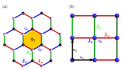
Figure 1: (a) Kitaev model on honeycomb lattice (HL). Red, green, blue colors label $J_{x,y,z}$ exchange interactions between black and white triangular sublattice sites. Yellow $\Phi_{l}=\eta_{\bf r}\eta_{{\bf r}^{\prime}}$ refers to the flux, with gauge fields $\eta_{\bf r},\eta_{{\bf r}^{\prime}}$ attached to blue edge of the hexagon. (b) Kitaev model, shrunk onto square lattice (SL) of Eq. (2). $J_{x,y}$ (red, green edges) mediate fermion hopping/pairing, along lattice vectors $\mathbf{e_{x,y}}$. Exchange interactions $J_{z}$ and gauge fields $\eta_{\bf r}$ (blue vertices) set on-site energy.

Our discussion of the thermal conductivity is based on calculations within linear response theory, assuming the long wave length limit $\mathbf{q}{\rightarrow}0$. For this, thermal transport coefficients are computed from the energy current auto-correlation functions $\langle{\cal J}(t){\cal J}\rangle$, where ${\cal J}$ is the energy current and $\langle\dots\rangle$ refers to the thermal trace FHM2007 . The real part of thermal conductivity, i.e. $\kappa^{\prime}(\omega)$, follows from the Fourier transform

$$C(\omega) = \frac{1}{N}\int dte^{i\omega t}\langle{\cal J}(t){\cal J}\rangle,$$ (3)

$$\kappa^{\prime}(\omega) = \frac{\beta}{2\omega}\left(1-e^{-\beta\omega}\right)\,C(\omega)\leavevmode\nobreak\ .$$ (4)

Generically, $\kappa^{\prime}(\omega)=2\pi D\delta(\omega)+\kappa^{reg}(\omega)$. The Drude weight (DW) $D$ refers to a ballistic channel, and if finite marks a perfect conductor. $\kappa^{reg}(\omega)$ encodes the dissipative parts of the heat flow. If $\kappa^{dc}=\kappa^{reg}(\omega\rightarrow 0)$ is finite, the system is a normal heat conductor with a finite DC conductivity. Interacting quantum systems with $D\neq 0$ are rare, see e.g. Ref. FHM2007 , and $D=0$ for $N\rightarrow\infty$ has also been argued for the Kitaev model Metavitsiadis2016 ; Metavitsiadis2017 . In turn, a prime goal of this work will be the analysis of $\kappa^{reg}(\omega)$ and its limit for $\omega\rightarrow 0$ in order to determine the DC conductivity.

To derive the heat current operator in (3) one has to realize that most of the gauge sectors in (2) are not translationally invariant, due to the real space distribution of $\eta_{\bf r}$. In turn, we employ the polarization operator $\mathbf{P}$ Metavitsiadis2017 , to obtain the current operator in real space

$$\mathbf{P}=\sum_{\mathbf{r}}\mathbf{r}h(\mathbf{r}),\,\,\,{\cal J}=\frac{\partial\mathbf{P}}{\partial t}=i\left[{\cal H},\mathbf{P}\right]\,.$$ (5)

It is worth noting, that in a translationally invariant system ${\cal J}$ from (5) is exactly identical to that obtained from the continuity equation in the limit of $\mathbf{q}{\rightarrow}0$. On the SL we get

$${\cal J}_{\mu}=2iJ_{\mu}\sum_{\mathbf{r}}[J_{z}\eta_{\mathbf{r}}\chi_{\mathbf{r}}\chi_{\mathbf{r}-\mathbf{e}_{\mu}}+\tau_{\mu}J_{\bar{\mu}}\chi_{\mathbf{r}}\chi_{\mathbf{r}+\mathbf{e}_{x}-\mathbf{e}_{y}}]\leavevmode\nobreak\ ,$$ (6)

with $\chi_{\mathbf{r}}=(d_{\mathbf{r}}^{\dagger}{+}d_{\mathbf{r}})$, $\bar{\mu}=y(x)$ and $\tau_{\mu}{=}+(-)$ for $\mu=x(y)$.

For the remainder of this work we resort to numerical methods to treat (3). For this we note, that not only the Hamiltonian, but also the current operator does not mediate transitions between gauge sectors. In turn, any thermal trace can be decomposed into a classical trace over gauges and a trace over the fermions, separately. For the latter, and for each fixed gauge sector $\{\eta\}=(\eta_{1},\dots,\eta_{N})$, we define a $2N$ component spinor $\mathbf{D}^{\dagger}=(d^{\dagger}_{1},\dots,d^{\dagger}_{N},d_{1},\dots,d_{N})$ of the fermions, with indices $1\dots N$ referring to the sites on the SL. With this the Hamiltonian and the current for each gauge sector read $\mathcal{H}=\mathbf{D^{\dagger}h(\eta)D}$, and ${\cal J}_{\mu}=\mathbf{D^{\dagger}j_{\mu}(\eta)D}$. Using a Bogoliubov transformation $U$ onto quasiparticle fermions $\mathbf{A}^{\dagger}=(a^{\dagger}_{1},\dots,a^{\dagger}_{N},a_{1},\dots,a_{N})$ via $\mathbf{A=U^{\dagger}D}$, the Hamiltonian is diagonalized as

$$\mathcal{H}=\sum_{i}\varepsilon_{i}(\{\eta\})(a^{\dagger}_{i}a_{i}-\frac{1}{2}),\$$ (7)

with quasiparticle energies $\varepsilon_{i}(\{\eta\})$. The contribution of each gauge sector to (3) can then be obtained straightforwardly by a Wick-decomposition of $\langle{\cal J}(t){\cal J}\rangle$ in the quasiparticle basis Metavitsiadis2016 .

III Results

In this section we will present our results for the dynamical energy current auto-correlation function $C(\omega,T)$ and the dc-limit of the heat conductivity $\kappa^{dc}(T)$ versus anisotropy at finite temperatures.

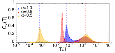
Figure 2: Specific heat $C_{\nu}(T)$ for $\alpha=1.0,0.8,0.5$ from ED on $N{=}6{\times}6$, i.e. 72 spinful sites versus $T$. Vertical lines at $T^{\star}_{\alpha}$ (blue dashed) and $T_{M}$ (red dashed) indicate temperature scales for flux and fermion entropy release.

III.1 Average gauge configuration method

Tracing over the gauge sectors in (3) can be done in various ways and to various degrees of precision. Among the methods are Markovian sampling of the gauges by QMC Motome2015b ; Motome2017 , exact summation over all gauges, equivalent to ED of the spin model Metavitsiadis2016 ; Metavitsiadis2017 , and summing only over a dominant subset of gauge configurations, i.e. the average gauge configuration (AGC) method Metavitsiadis2016 ; Metavitsiadis2017 , which will be used here. The following sketches the main ideas of the AGC method, while for more details we refer the reader to Refs. Metavitsiadis2016 ; Metavitsiadis2017 . The notion of an average gauge configuration is trivial in the low- and the high-temperature limit. In the former, the gauges assume a flux-free configuration Kitaev2006 , and in the latter a typical gauge configuration is fully random. These limiting cases are separated by a temperature scale $T^{\star}_{\alpha}$ at which flux-proliferation occurs upon increasing temperature. Here $\alpha$ refers to the anisotropy parameter. $T^{\star}_{\alpha}$ scales with the energy to excite a single flux, i.e. the flux gap $\Delta_{\Phi}/J\ll 1$ Kitaev2006 . Because of the latter inequality, $T^{\star}_{\alpha}$ and the crossover regime can be read off from the specific heat, i.e. from the entropy release of the gauge fields Motome2015b , since this is well separated from the fermionic energy scales $O(J)$. Our strategy will be to first determine $T^{\star}_{\alpha}$ and then to confine all evaluations of $C(\omega)$ to temperatures above this scale, such that averaging over only completely random gauge states is sufficiently justified for the gauge trace. Consequently, the remaining effective fermionic model is a binary disorder problem. It turns out that the temperature range accessible by this approach is large enough for our purposes.

To approximate $T^{\star}_{\alpha}$ we now calculate the specific heat $C_{\nu}(T)=T\partial S/\partial T$ noteSpec . This is done exactly on finite systems, tracing over both, fermions and gauges. The system sizes we can reach for this, namely $N{\leq}6{\times}6$, i.e. 72 spins, are larger than those for exact thermodynamics using the many body spin basis, however, still much smaller than those which will be used within the AGC subsequently. Fig. 2 shows the temperature dependence of the specific heat for three different values of anisotropy. As expected, two peaks develop at two different temperature scales, corresponding to the release of entropy from the gauge degrees of freedom and the mobile Majorana fermions, at $T^{\star}_{\alpha}$ and $T_{M}/J{\sim}1$, respectively. Obviously, the global fermionic energy scale $J$ is only weakly affected by the gauge disorder, and therefore the high-$T$ peak remains rather insensitive to $\alpha$. However the low-$T$ peak at $T^{\star}_{\alpha}$ is strongly shifted to smaller temperatures, by roughly two orders of magnitude, upon decreasing $\alpha$ from 1 to 0.5. This finding is consistent with results from QMC Motome2015b . While in principle $T^{\star}_{\alpha}$ sets an individual temperature scale for each $\alpha$, above which averaging over fully random gauge configurations provides a sufficient approximation for the gauge trace, we will use the maximum of these, i.e. $T^{\star,\mathrm{max}}_{\alpha}/J\sim O(.1)$ as the lowest temperature to apply the AGC for all subsequent calculations, independent of $\alpha$.

III.2 Dynamical current correlations

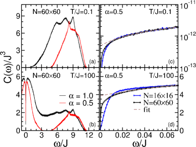
Figure 3: $C(\omega)$ from the AGC method, versus $\omega$ for two temperatures, $T/J=0.1$ (a,c) and $100$ (b,d). (a,b): Variation with anisotropy for $\alpha=1,0.5$ (black, red), corresponding to the gapless and gapful phase on a large $\omega$-scale for $N{=}60{\times}60$ sites. (c,d): Variation with system size $N{=}16{\times}16,60{\times}60$ (blue, black) at low-$\omega$ for $\alpha=0.5$. Brown dashed line: fitting-polynomial for $C(\omega,N{=}60{\times}60)$ to extract $\kappa^{dc}(T)$.

Now we turn to the dynamical current correlation function $C(\omega)$. Results on up to 60$\times$60-sites systems are displayed in Fig. 3 for two representative anisotropy values $\alpha=1.0(0.5)$. These place the system into the gapless(ful) phase. Two temperatures, i.e. $T/J{=}0.1,100$ are shown, which allow to highlight the difference between low and high matter fermion densities. We begin with Fig. 3(a). Here the fermion occupation number at all momenta is small and the intensity is essentially due to two-fermion pair-breaking contributions to $C(\omega)$. For $\alpha=0.5$, the one-particle dispersion displays a gap $\Delta$, at $\Delta/J\approx 2$ Motome2015b , with a corresponding two-particle excitation gap $\xi$ in $C(\omega)$ at $\xi/J\approx 4$. Moving to Fig. 3(b) the matter-fermion density is large and direct transport by thermally populated quasiparticle states contributes. In a clean system this transport would show up as a Drude peak strictly at $\omega{=}0$. Due to the gauge disorder however, the Drude peak is smeared over a substantial range of finite frequencies $\sim O(J)$. Interestingly, the randomness provided for by the gauge field is not sufficient to fill in the gap completely, as is obvious from panel (a) and (b). Related observations have been made in Refs. Motome2015b ; Motome2016 . The ’smeared Drude peak’ in Fig. 3(b) features a very narrow zero-frequency dip, which requires careful finite size analysis. Examples of such analysis are shown in Fig. 3(c,d) for the case of $\alpha=0.5$. The main point can be read off best from panel (d), where it is amply clear, that as $N\rightarrow\infty$ the zero-frequency dip closes in onto the y-axis. This observation renders the system a normal, dissipative heat conductor in the thermodynamic limit and extends identical findings from Ref. Metavitsiadis2017 to the case of $\alpha\neq 1$. Note, that there is a difference of several orders of magnitude between $C(\omega)$ in Figs. 3(c) and 3(d). This is related to the thermal activation behavior in the gapful case, to be discussed in the next section.

III.3 DC-limit of heat conductivity

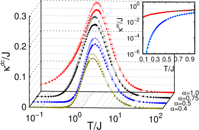
Figure 4: Thermal conductivity $\kappa^{dc}$ versus $T$ for various values of anisotropies $\alpha=1.0\dots 0.4$, shown on the lower right axis, ranging from the gapless to gapped phases. Two system sizes, $N{=}16{\times}16$ (dashed with empty circles), and $N{=}60{\times}60$ (solid with solid circles), are compared. Inset: low-$T$ behavior for $\alpha=1.0$ (red dots) and $0.5$ (blue dots) superimposed onto two distinct fit functions $T^{\gamma}$, with $\gamma{=}0.92$ (black solid) and $e^{-\Delta/T}$, with $\Delta{=}2.30$ (blue solid), for $N{=}60{\times}60$.

Based on a series of calculations as in Fig. 3, we have extrapolated the dc-limit $C(\omega\rightarrow 0,T,\alpha)$ over a wide range of $T$ and $\alpha$, sufficient to acquire a consistent picture of the thermal conductivity $\kappa^{dc}(T,\alpha)$ both, in the gapless and the gapful regime. This result is depicted in Fig. 4. To arrive at this, the brown dashed lines in Fig. 3(c,d) exemplarily indicate the extrapolation procedure performed, for each of the largest systems, i.e. for $N{=}60{\times}60$. It consists of least-square fitting of the low-$\omega$ range of the correlation function for each pair of $T,\alpha$ by second order polynomials, from which the dc value $C(\omega\rightarrow 0,T)$ is extracted. We have chosen a range of $0.02\leq\omega/J\leq 0.12$ to determine the coefficients of the polynomial in all cases. To obtain some form of finite-size scaling, we have compiled the results of the fitting procedure for two system sizes, i.e. $N{=}L{\times}L$ and $L{=}\{16,60\}$, into Fig. 4, showing dashed (solid) curves with empty (solid) circles, for $L{=}16(60)$. Although the linear dimension of the systems shown differs by almost a factor of 4, $\kappa^{dc}$ displays only minimal differences for most of the temperatures. Only around $T/J\approx 1$, a small, systematic correction towards lower values with increasing system size is observed for every $\alpha$. This implies visible, but satisfyingly little finite-size effects, presumably putting the largest system sizes rather close to the thermodynamic limit.

Fig. 4 is a main result of this paper. It extends previous analysis of the thermal conductivity of the Kitaev model Motome2017 ; Metavitsiadis2017 into the anisotropic regime. It demonstrates a qualitative change of the temperature dependence of $\kappa^{dc}(T,\alpha)$, as the system crosses over from the gapless to the gapful spectrum. In the former the thermal conductivity roughly scales with a power law, $\kappa^{dc}\sim T^{\gamma}$ for $T/J\ll 1$, while in the latter an exponential behavior with $\kappa^{dc}\sim\exp(-\Delta/T)$ provides a reasonable description. This is in line with the notion of quasiparticle transport, since the activation gap $\Delta$ is consistent with the one-particle gap, e.g. $\Delta/J\sim 2$ for $\alpha=0.5$ as discussed in Sec. III.2.

We would like to emphasize, that while the trend of the curves in Fig. 4 might suggest a strictly vanishing $\kappa^{dc}$, e.g. for $\alpha\geq 0.5$ and $T/J\lesssim 0.5$, this is not so, based on our results. Rather, the y-axis scale in Fig. 3(c) is very small, albeit finite. Such small orders of magnitude are consistent with the rapid low temperature suppression by the exponential activation. In turn, our findings suggest, that the Kitaev model is a normal dissipative heat conductor at all finite temperatures, at least above $T^{\star}_{\alpha}$, for all $\alpha$.

IV Conclusion

In summary, we have investigated the longitudinal dynamical thermal conductivity of the Kiteav model on the honeycomb lattice with anisotropic exchange couplings. Using an average gauge configuration method, combined with exact diagonalization of the matter fermion sector, systems of up 7200 spinful sites have been analyzed over a wide range of temperatures and anisotropies. We have confirmed both, the applicability and range of validity of our method by complementary exact analysis of thermodynamic properties. Our main finding is that for all temperatures and anisotropies investigated, the systems feature normal dissipative transport, consistent with scattering of the matter fermions from the static fluxes, and also consistent with a temperature dependence set by the matter fermion mass gap. From an experimental point of view, transport in putative Kitaev quantum spin liquids could be interesting under strain in order to tune exchange couplings, while monitoring the temperature dependence of thermal transport.

V Acknowledgments

We thank M. Vojta and C. Hess for comments and discussion. Work of A.P. and W.B. has been supported in part by the DFG through SFB 1143, project A02. Work of W.B. has been supported in part by QUANOMET and the NTH-School CiN. W.B. also acknowledges kind hospitality of the PSM, Dresden. This research was supported in part by the National Science Foundation under Grant No. NSF PHY-1748958.

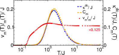
Figure 5: Red solid circles: $\kappa^{dc}(T)/C_{m}(T)\equiv v_{m}(T)\ell_{m}(T)$. versus $T$ at $\alpha=0.5$. Solid lines with solid circles: $\kappa^{dc}(T)$ (blue) and $C_{m}(T)$ (yellow) evaluated by AGC method on $N=32\times 32$ sites.

Appendix A Kinetic model of thermal conductivity

This appendix is a digression into phenomenology, which we add out of curiosity. It is customary to perform kinetic modeling of thermal conductivities, expressing $\kappa^{dc}(T)$ in terms of quasiparticle properties Hess2018a ; Hess2001

$$\kappa^{dc}(T)\approx\sum_{k,p}C_{k,p}(T)v_{k,p}(T)\ell_{k,p}(T)\,,$$ (A.1)

where $C_{k,p}(T),v_{k,p}(T)$, and $\ell_{k,p}(T)$ refer to the specific heat, velocity, and mean free path at momentum $k$ of quasiparticles of type ’$p$’. In the present case these types are fluxes, $p{=}f$, and matter fermions, $p{=}m$. Disentangling the contributions to $\kappa^{dc}(T)$ from various types ’$p$’ is only an option, if their spectral supports are well separated. As one can read off directly from Fig. (2), exactly this is possible for strong anisotropy, e.g. $\alpha=0.5$, where the flux peak in $C_{\nu}(T)$ at $T^{\star}_{\alpha}$ is well separated from the dominant contributions to the specific heat of the fermions. Moreover, realizing that the flux velocity $v_{k,f}=0$, and adopting the usual approximation to drop the momentum summation in (A.1) in favor of momentum integrated quantities, one gets $\kappa^{dc}(T)\sim C_{m}(T)v_{m}(T)\ell_{m}(T)$ for $T>T^{\star}_{\alpha}$.

From this it is tempting to analyze the ratio of $\kappa^{dc}(T)/C_{m}(T)$, as obtained from our calculations, e.g. for $\alpha=0.5$. This is shown in Fig. 5. It is this variation of $v_{m}(T)\ell_{m}(T)$ with $T$, which this appendix is meant to speculate on as follows. First, at all $T>T^{\star}_{\alpha}$, the flux lattice is completely random, setting a mean free path for the fermions, independent of $T$. Second, for sufficiently large $T$, fermions far up in the Dirac cone set the Fermi velocity, which is also independent of $T$. Third, upon lowering $T$, fermions close to the gap set $v_{m}(T)$. This velocity approaches zero as $T\rightarrow 0$. Remarkably, these points are roughly captured in the temperature variation of $v_{m}(T)\ell_{m}(T)$, seen in Fig. 5.

References

- (1) L. Balents, Nature 464, 199-208 (2010).
- (2) L. Savary and L. Balents, Rep. Prog. Phys. 80, 016502 (2017).
- (3) A. Kitaev, Ann. Phys. (N.Y.) 321, 2 (2006).
- (4) X.-Y. Feng, G.-M. Zhang, and T. Xiang, Phys. Rev. Lett. 98, 087204 (2007).
- (5) H.-D. Chen and Z. Nussinov, J. Phys. A: Math. Theor. 41, 075001 (2008).
- (6) Z. Nussinov and G. Ortiz, Phys. Rev. B 79, 214440 (2009).
- (7) S. Mandal, R. Shankar and G. Baskaran, J. Phys. A: Math. Theor. 45, 335304 (2012).
- (8) G. Khaliullin, Prog. Theor. Phys. Suppl. 160, 155 (2005).
- (9) G. Jackeli and G. Khaliullin, Phys. Rev. Lett. 102, 017205 (2009).
- (10) J. Chaloupka, G. Jackeli, and G. Khaliullin Phys. Rev. Lett. 105 027204 (2010).
- (11) Z. Nussinov and J. van den Brink, Rev. Mod. Phys. 87, 1 (2015).
- (12) S. Trebst, arXiv:1701.07056.
- (13) A. Banerjee, C. A. Bridges, J. Q. Yan, A. A. Aczel, L. Li, M. B. Stone, G. E. Granroth, M. D. Lumsden, Y. Yiu, J. Knolle, S. Bhattacharjee, D. L. Kovrizhin, R. Moessner, D. A. Tennant, D. G. Mandrus, and S. E. Nagler, Nat. Mater. 15, 733 (2016).
- (14) A. Banerjee, J. Yan, J. Knolle, C. A. Bridges, M. B. Stone, M. D. Lumsden, D. G. Mandrus, D. A. Tennant, R. Moessner, and S. E. Nagler, Science 356, 6342 (2017).
- (15) A. Banerjee, P. Lampen-Kelley, J. Knolle, C. Balz, A. A. Aczel, B. Winn, Y. Liu, D. Pajerowski, J. Yan, C. A. Bridges, A. T. Savici, B. C. Chakoumakos, M. D. Lumsden, D. A. Tennant, R. Moessner, D. G. Mandrus, and S. E. Nagler, Nat. Part. J. Quantum Mater. 3, 8 (2018).
- (16) J. Knolle, G.W. Chern, D.L. Kovrizhin, R. Moessner, and N.B. Perkins, Phys. Rev. Lett. 113, 187201 (2014).
- (17) S.-H. Baek, S.-H. Do, K. Y. Choi, Y.S. Kwon, A.U.B. Wolter, S. Nishimoto, J. van den Brink, and B. Büchner, Phys. Rev. Lett. 119, 037201 (2017).
- (18) J. Zheng, K. Ran, T. Li, J. Wang, P. Wang, B. Liu, Z.-X. Liu, B. Normand, J. Wen, and W. Yu, Phys. Rev. Lett. 119, 227208 (2017).
- (19) C. Hess, arXiv:1805.01746.
- (20) K. W. Plumb, J. P. Clancy, L. J. Sandilands, V. V. Shankar, Y. F. Hu, K. S. Burch, H.-Y. Kee, and Y.-J. Kim, Phys. Rev. B 90, 041112 (2014).
- (21) D. Hirobe, M. Sato, Y. Shiomi, H. Tanaka, E. Saitoh, Phys. Rev. B 95, 241112 (2017).
- (22) I.A. Leahy, C.A. Pocs, P.E. Siegfried, D. Graf, S.-H. Do, K.-Y. Choi, B. Normand, and M. Lee, Phys. Rev. Lett. 118, 187203 (2017).
- (23) R. Hentrich, A. U. B. Wolter, X. Zotos, W. Brenig, D. Nowak, A. Isaeva, T. Doert, A. Banerjee, P. Lampen-Kelley, D. G. Mandrus, S. E. Nagler, J. Sears, Y.-J. Kim, B. Büchner, C. Hess, Phys. Rev. Lett. 120, 117204 (2018).
- (24) Y. J. Yu, Y. Xu, K. J. Ran, J. M. Ni, Y. Y. Huang, J. H. Wang, J. S. Wen, and A. Y. Li, Phys. Rev. Lett. 120, 067202 (2018).
- (25) Y. Kasahara, T. Ohnishi, Y. Mizukami, O. Tanaka, S. Ma, K. Sugii, N. Kurita, H. Tanaka, J. Nasu, Y. Motome, T. Shibauchi, and Y. Matsuda, Nature 559, 227-231 (2018).
- (26) J. Nasu, J. Yoshitake, and Y. Motome, Phys. Rev. Lett. 119, 127204 (2017).
- (27) R. Steinigeweg and W. Brenig, Phys. Rev. B 93, 214425 (2016).
- (28) A. Metavitsiadis and W. Brenig, Phys. Rev. B 96, 041115(R) (2017).
- (29) A. Metavitsiadis, A. Pidatella, and W. Brenig, Phys. Rev. B 96, 205121 (2017).
- (30) A. Metavitsiadis, C. Psaroudaki, and W. Brenig, arXiv:1806.02344.
- (31) G. L. Stamokostas, P. E. Lapas, and G. A. Fiete, Phys. Rev. B 95, 064410 (2017).
- (32) F. Heidrich-Meisner, A. Honecker, and W. Brenig, Eur. Phys. J. Special Topics 151, 135 (2007).
- (33) J. Nasu, M. Udagawa, and Y. Motome, Phys. Rev. B 92, 115122 (2015).
-
(34)
The specific heat is evaluated numerically via temperature derivative of entropy
is the thermal energy of the matter fermions in a particular configuration, with the single-particle energy, and the free energy of the matter fermions. Here is the total partition function.(A.2) - (35) J. Nasu, and Y. Motome, Phys. Conf. Ser. 683, 012037 (2016).
- (36) C. Hess, C. Baumann, U. Ammerahl, B. Büchner, F. Heidrich-Meisner, W. Brenig, and A. Revcolevschi, Phys. Rev. B 64, 184305 (2001).