Evolutionary aspects of Reservoir Computing

Abstract

Reservoir Computing (RC) is a powerful computational paradigm that allows high versatility with cheap learning. While other artificial intelligence approaches need exhaustive resources to specify their inner workings, RC is based on a reservoir with highly non-linear dynamics that does not require a fine tuning of its parts. These dynamics project input signals into high-dimensional spaces, where training linear readouts to extract input features is vastly simplified. Thus, inexpensive learning provides very powerful tools for decision making, controlling dynamical systems, classification, etc. RC also facilitates solving multiple tasks in parallel, resulting in a high throughput. Existing literature focuses on applications in artificial intelligence and neuroscience. We review this literature from an evolutionary perspective. RC’s versatility make it a great candidate to solve outstanding problems in biology, which raises relevant questions: Is RC as abundant in Nature as its advantages should imply? Has it evolved? Once evolved, can it be easily sustained? Under what circumstances? (In other words, is RC an evolutionarily stable computing paradigm?) To tackle these issues we introduce a conceptual morphospace that would map computational selective pressures that could select for or against RC and other computing paradigms. This guides a speculative discussion about the questions above and allows us to propose a solid research line that brings together computation and evolution with RC as a working bench.

I Introduction

Somewhere between pre-biotic chemistry and the first complex replicators, information assumed a paramount role in our planet’s fate SzathmaryMaynardSmith1997 ; Joyce2002 ; WalkerDavies2013 . From then onwards, Darwinian evolution explored multiple ways to organize the information flows that shape the biosphere Schuster1996 ; Smith2000 ; JablonkaLamb2006 ; Nurse2008 ; Joyce2012 ; Adami2012 ; HidalgoMaritan2014 ; SmithMorowitz2016 . As Hopfield argues, “biology looks so different” because it is “physics plus information” Hopfield1994 . Central in this view is the ability of living systems to capitalize on available external information and forecast regularities from their environment Jacob1998 ; Wagensberg2000 , a driving force behind life’s progression towards more complex computing capabilities SeoaneSole2018a .

We can trace computation in biology from pattern recognition in RNA and DNA PaunSalomaa2005 ; Doudna2017 (figure 1a), through the Boolean logic implemented by interactions in Gene Regulatory Networks Thomas1973 ; Kauffman1996 ; RodriguezCasoSole2009 (figure 1a), to the diverse and versatile circuitry implemented by nervous systems of increasing complexity DayanAbbott2001 ; Seung2012 (figure 1c-e). Computer Science, often inspired by biology, has reinvented some of these computing paradigms; usually from simplest to most complex, or guided by their saliency in natural systems. It is no surprise that we find some fine-tuned, sequential circuits for motor control (figure 1c) that resemble the wiring of electrical installations. Such pipelined circuitry gets assembled to perform parallel and more coarse-grained operations, e.g., in assemblies of ganglion retinal cells that implement edge detection Levick1967 ; RussellWerblin2010 (figure 1d) similarly to filters used in image processing MarrHildreth1980 ; Marr1982 ; StephensBialek2013 . Systems at large often present familiar design philosophies or overall architectures, as illustrated by the resemblance between much of our visual cortex (figure 1e) and deep convolutional neural networks for computer vision FukushimaMiyake1982 ; KrizhevskyHinton2012 ; YaminsDiCarlo2014 ; KhalighRazaviKriegeskorte2014 (figure 1f).

Such convergences suggest that chosen computational strategies might be partly dictated by universal pressures. We expect that specific computational tricks are readily available for natural selection to exploit them (e.g. convolving signals with a filter is faster in Fourier space, and the visual system could take advantage of it). Such universalities could constrain network structure in specific ways. We also expect that the substrate chosen for implementing those computations is guided by what is needed and available. This is, at large, one of the topics discussed in this volume. Different authors explore specific properties of computation as implemented, on the one hand, by liquid substrates with moving components such as ants or T-cells; and, on the other hand, by solid brains such as cortical or integrated circuits. Rather than this ‘thermodynamic state’ of the hardware substrate, this paper reviews the Reservoir Computing (RC) framework Jaeger2001 ; MaassMarkram2002 ; JaegerPrincipe2007 ; VerstraetenStroobandt2007 ; LukoseviciousSchrauwen2012 , which somehow deals with a ‘solid’ or ‘liquid’ quality of the signals involved; hence rather focusing on the ‘state’ of the software. As with other computing architectures, tricks, and paradigms, we expect that the use of RC by Nature responds to evolutionary pressures and contingent availability of resources.

RC matters within a broader historical context because it has helped bypass a huge problem in machine learning. The first widely successful artificial intelligence architecture were layered, feed-forward networks (figure 1f and KrizhevskyHinton2012 are modern examples). These get a static input (e.g. a picture) whose basic features (intensity of light in each pixel) are read and combined by artificial neurons or units. A neuron’s reaction, or activation, is determined by a collection of weights that measure how much each of the features matters to that unit. These activations are conveyed forward to newer neurons that use their own weights to combine features non-linearly, and thus extract complex structures (edges, shapes, faces, …). Eventually, the whole network settles into a fixed state. A set of output units returns the static result of a computation (e.g. whether Einstein is present in the picture). Training a network consists in adjusting the weights for every neuron such that the system at large implements a desired computation (e.g. automatic face classification). Solving this problem in feed-forward networks with several layers was a challenge for decades until a widespread solution (back-propagation RumelhartWilliams1986 ) was adopted. Recurrent Neural Networks (RNN) brought in more computational power to the field. RNN contemplate feedback from more forward to earlier processing neurons. These networks do not necessarily settle in static output states, allowing them to produce dynamic patterns, e.g. for system control. They are also apt to process spatiotemporal inputs (videos, voice recordings, temporal data series, …), finding dynamical patterns often with long-term dependencies. Echoing the early challenges in feed- forward networks, full RNN training (i.e. adjusting every weight optimally for a desired task) presents important problems still not fully tamed BengioFrasconi1994 ; PascanuBengio2018 .

RC is an approach that vastly simplifies the training of RNN, thus making more viable the application of this powerful technology. Instead of attempting to adjust every weight in the network, RC considers a fixed reservoir that does not need training (figure 2a) which works as if multiple, parallel spatiotemporal filters were simultaneously applied onto the input signal. This effectively projects non-linear input features onto a huge-dimensional space. There, separating these features becomes a simple, linear task. Despite the simplicity of this method, RC-trained RNN have been robustly used for a plethora of tasks including data classification VerstraetenStroobandt2006 ; JaegerSiewert2007 ; SoriaRuffini2018 , systems control JoshiMaass2004 ; SalmenPloger2005 ; Burgsteiner2005 ; JaegerSiewert2007 , time-series prediction JaegerHaas2004 ; IbanezSoriaRuffini2018 , uncovering grammar and other linguistic and speech features VerstraetenVanCampenhout2005 ; JaegerSiewert2007 ; TongCottrell2007 ; TriefenbachMartens2010 ; HinautDominey2013 etc.

Again, we expect that Nature has taken advantage of any computing approaches available, including RC, and that important design choices are affected by evolutionary constraints. These will be major topics through the paper: how could RC be exapted by living systems and how might evolutionary forces have shaped its implementation. Section II provides a brief introduction to RC and reviews what its operating principles (notably optimal reservoir design) imply for biological systems. Section III shows inspiring examples from biology and engineering. Comments on selective forces abound across the paper, but section IV wraps up the most important messages. This last part is largely speculative in an attempt to pose relevant research questions and strategies around RC, evolution, and computation. We will hypothesize about two important topics: i) what explicit evolutionary conditions might RC demand and ii) what evolutionary paths can transform a system into a reservoir.

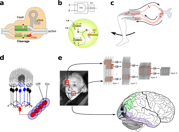
Figure 1: Some computing devices in biology. a DNA and RNA performs multiple pattern recognition, starting with the simplest matching of codons in ribosomes to synthesize proteins. More complex pattern matching (here, Cas9 matches a longer string of RNA to DNA, drawing from Marius Walter available at https://commons.wikimedia.org/w/index.php?curid=62766587) allows cleavage and insertion of DNA snippets. b Boolean logic determines gene expression or silencing. In the example, a receptor gene that expresses GFP is only active if genes A and B are expressed and their corresponding products dimerize. This implements a Boolean AND gate. (Redrawn from MaciaSole2014 .) c The knee jerk reflex is implemented by sequential circuits that remind us of the simple wiring of an electrical installation. Sensory neurons (A) gather a sudden input. Information follows the arrows towards ganglia at the entrance (B) and gray matter of the spinal cord. There, information splits in two: it is partially sent upstream towards the brain stem (not shown) and partially used to excite motor neurons (C) which right away pull from muscles at their end (D). d Retinal ganglion cells (red) pool information from rods and cones (gray) through horizontal, bipolar (black and blue), and amacrine cells. This pooling involves excitatory (blue) and inhibitory (black) mediating connections, which make a ganglion cell responsive to light and its absence in so-called on- and off- centers and surround (red and blue discs, corresponding to dark and light gray cones). Receptive fields of several ganglia are consequently pooled as well, resulting in edge detectors. e Specific neurons implementing average and pooling exist throughout the visual cortices FukushimaMiyake1982 . These are the building blocks of deep convolutional neural networks KrizhevskyHinton2012 . The overall information flow, architecture, and various receptive fields of such artificial networks reminds several processing steps found in mammal visual cortices YaminsDiCarlo2014 , including edge detection in V1 thanks to retinal ganglia. (This image was drawn with elements from YaminsDiCarlo2014 and https://commons.wikimedia.org/w/index.php?curid=1679336.)

II Computational aspects of Reservoir Computing

II.1 Reservoir Computing in a nutshell

RC was simultaneously introduced by Herbert Jaeger Jaeger2001 and Wolfgang Maass and his colleagues MaassMarkram2002 . Jaeger arrived to Echo State Networks from a machine learning approach while Maass et al. developed Liquid State Machines with neuroscientifically realistic spiking neurons. The powerful operating principle is the same behind both approaches, later unified under the RC label JaegerPrincipe2007 ; VerstraetenStroobandt2007 ; LukoseviciousSchrauwen2012 .

Consider a Recurrent Neural Network (RNN) consisting of $N$ units, all connected to each other, which receive an external input $\bar{y}^{in}(t)\equiv\{y^{in}_{i}(t),\>i=1,\dots,N\}$ (with $y^{in}_{i}(t)=0$ if the $i$-th unit receives no input). Each unit has an internal state $x_{i}(t)$ that evolves following:

$$x_{i}(t+\Delta t) = \sigma\left(\sum_{j=1}^{N}\omega_{ij}x_{j}(t)+y^{in}_{i}(t)\right),$$ (1)

where $\sigma(\cdot)$ represents some non-linear function (e.g. an hyperbolic tangent). Variations of this basic theme appear in the literature. For example, continuous dynamics based on differential equations could be used; or inputs could consist of weighted linear combinations of $N^{feat}$ more fundamental features $\{u_{k}(t),k=1,\dots,N^{feat}\}$ such that $y^{in}_{i}(t)=\sum_{k=1}^{N^{feat}}\omega^{in}_{ik}u_{k}(t)$. This would allow us to trade off importance of external stimuli versus internal dynamics.

Such RNN can be trained so that $N^{out}$ designated output units produce a desired response $\bar{y}^{out}(t)\equiv\{y_{i}^{out}(t),\>i=1,\dots,N^{out}\}$ when $\bar{y}^{in}(t)$ is fed into the network. The training consists in varying the $\omega_{ij}$ until the state of the output units given the input $\bar{x}^{out}(t|\bar{y}^{in}(t))\equiv\{x^{out}_{i}(t|\bar{y}^{in}(t)),\>i=1,\dots,N^{out}\}$ matches the desired behavior $\bar{y}^{out}(t)$. A naive approach is to initialize the $\omega_{ij}$ randomly and modify all weights, e.g. using gradient descent, to minimize some error function $\epsilon(\bar{y}^{out}(t),\bar{x}^{out}(t|\bar{y}^{in}(t)))$ that measures how much does the network activity deviate from the target. Such training procedure is often useless because the RNN’s recurrent dynamics introduce insurmountable numerical problems BengioFrasconi1994 ; PascanuBengio2018 .

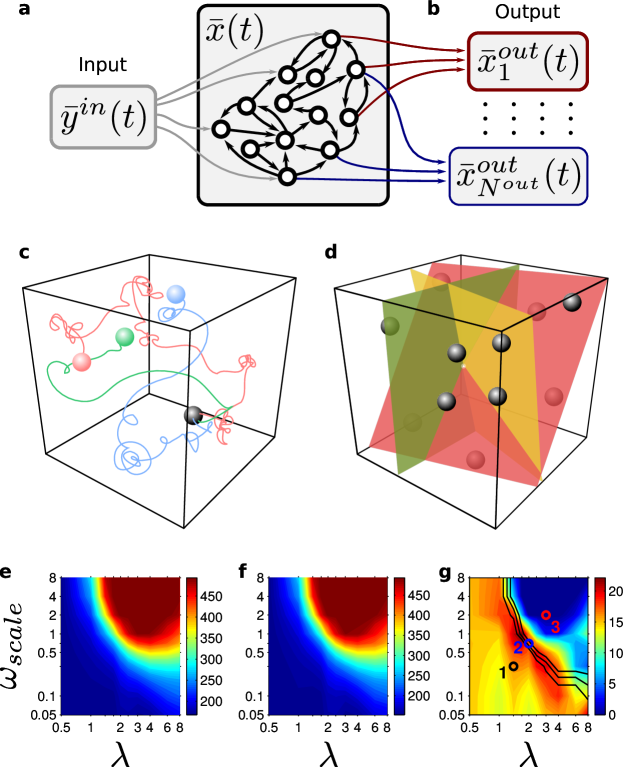
Figure 2: Computational basis of reservoir computing. a Reservoir dynamics (black nodes and arrows) are driven by external inputs (gray arrows). For RC, weights within the reservoir are not modified. b A set of $N^{out}$ output nodes can be appended. Each of them computes a linear combination of the reservoir state and solves a single task. In RC training, only the weights of these output units are modified. This allows us to solve several (in this case $N^{out}$) different tasks simultaneously without interference. c The key to RC computing is that the reservoir filters, and thus projects, low-dimensional input signals into a huge-dimensional space. Here we observe three example trajectories (elicited, e.g., by three different inputs) through a representation of this abstract space. d Appropriate reservoir dynamics will make it possible to separate the projection of different inputs using simple linear classifiers (implemented by the readout units from b). If we sort in a matrix the different dynamical states reached after different inputs, the rank of this matrix tells us how linearly independent the dynamics have remained. This gives us an idea of how many different hyperplanes (i.e., readouts and different tasks) we can draw in this abstract space. e-g $r^{S}$, $r^{G}$, and $r^{S}-r^{G}$. Plot reproduced from LegensteinMaass2007b . e $r^{S}$, which captures this separability property, is plotted for reservoirs made of simulated cortical columns with varying correlation length between neurons ($\lambda$) and scale of synaptic strength ($\omega_{scale}$). We find large $r^{S}$ (hence large separability) for chaotic dynamics achieved by large $\lambda$ and $\omega_{scale}$. f When noise and redundant information has been provided, we expect the rank of a similar matrix ($r^{G}$, which measures a generalization capability) to score low. The same microcolumns as before present good generalization property when the dynamics are ordered and similar inputs are consistently mapped into a same region of the space of reservoir dynamics. g Subtracting $r^{G}$ from $r^{S}$ measures a balance between the two desired reservoir properties. Good performance also correlates with a measure of criticality (dot marked ‘2’, where the Lyapunov exponent vanishes). Performance is bad for too ordered (dot ‘1’, negative Lyapunov exponent) or too chaotic dynamics (dot ‘3’, positive Lyapunov exponent). Black curves on top indicate the limits where Lyapunov exponents are fairly close to $0$, thus marking the edge of chaos.

The RC approach to RNN training still uses random $\omega_{ij}$ but does not attempt to modify them. We say then that the units described by equation 1 constitute a reservoir (figure 2a). Upon it, we append a set of $N^{out}$ readout units (figure 2b) whose activity $\bar{x}^{out}(t)\equiv\{x^{out}_{i}(t),\>i=1,\dots,N^{out}\}$ is just a linear combination of the reservoir activity:

$$x^{out}_{i}(t) = \sum_{j=1}^{N}\omega^{out}_{ij}x_{j}(t).$$ (2)

Training proceeds on these output units alone. Only the $\omega^{out}_{ij}$ are modified; these do not feed back into the reservoir, which remains unchanged. The absence of this feedback during learning dissolves the grave numerical problems that affect other RNN. Finding the right $\omega^{out}_{ij}$ for a task becomes as simple as a linear regression between reservoir activity over time given an input $x_{j}(t|\bar{y}^{in}(t))$ and the desired target $\bar{y}^{out}(t)$ WyffelsStroobandt2008 . For a review on RC training (including issues of reservoir design discussed in the next section) see LukoseviciousJaeger2009 and other works Jaeger2002 ; Lukosevicious2012 . Also, the computational capacity of RC can be boosted if a (trainable) feedback is added from the linear readouts to the reservoir MaassSontag2007 ; SussilloAbbott2009 ; DaiHarley2009 ; RivkindBarak2017 ; CeniLivi2018 . This allows for more agile context-dependent computations and longer-term memory MaassSontag2007 . Controlling the network attractors (thus the learning) that such feedback induces is still not fully understood. These and other variations upon the RC theme are good steps towards full RNN training.

Back to the most naive version of RC, the only task of the reservoir is to have its dynamic internal state perturbed by the input. In doing so, through its non-linear, convoluted dynamics, the reservoir is picking up the external signal and projecting it into the huge-dimensional space that consists of all possible dynamic configurations of the reservoir (figure 2c). This high-dimensional space hopefully renders relevant features from the input more easily separable. Ideally, such features could be separated with a simple hyperplane that bisects this abstract space. This is precisely what the $\omega^{out}_{ij}$ implement. RC training consists in finding the right hyperplane solving each task given the reservoir.

Of course, very poor dynamics could project inputs into boring reservoir configurations so that prominent features cannot be picked up. Next section discusses issues of reservoir design so that it produces optimal dynamics. However, the most important part of the training falls upon the readouts, whose dynamics do not affect the reservoir. This brings in the two most important advantages of RC: i) Learning is extremely easy, as just discussed, and ii) multiple readouts can be appended to a same reservoir (thus solving different, parallel tasks) without interference.

II.2 Good reservoir design: separability, generalization, criticality, and chaos

When RC was first introduced, it was requested that the reservoir dynamics fulfilled a series of theoretical conditions such as presenting echo states, fading memory, separation property, etc Jaeger2001 ; MaassMarkram2002 . These are formal requirements to prove relevant computational theorems. In practice, a wide variety of systems can trivially work as reservoirs. As proofs of concept, among many others, in silico implementations have used realistic theoretical models of neural networks MaassMarkram2002 ; MaassBertschinger2005 ; LegensteinMaass2007b , networks of springs HauserMaass2011 ; NakajimaPfeifer2013a , or cellular automata NicheleGundersen2017 ; and in hardware, analog circuits SorianoVanDerSande2015 ; DuLu2017 , a bucket of water FernandoSojakka2003 , and diverse photonic devices AppletantFischer2011 ; PaquotMassar2012 ; VandoorneBienstman2014 have been tried. All those theoretical conditions on reservoir dynamics boil down to two desired properties: i) reservoir dynamics must be able to separate different input features that are meaningful for a variety of tasks while ii) these same dynamics must be able to generalize to unseen examples, thus projecting reasonably similar inputs into a reasonable neighborhood within the dynamical space of the reservoir. To fulfill these conditions we want our reservoirs to behave somehow in between chaotic and simple dynamics, thus resonating with ideas about criticality in complex systems, as discussed below.

In a series of papers MaassBertschinger2005 ; LegensteinMaass2007b ; LegensteinMaass2007a , Maass et al. explored two elegant measures that quantify the ability of a reservoir to separate relevant features and to generalize to unseen examples.

Regarding separability, since RC works with simple linear readouts, we can quantify straightforwardly how many different binary features can be extracted by hyperplanes that bisect the space of dynamic configurations of the reservoir (figure 2d). Suppose a collection of inputs $Y^{S}\equiv\{y^{S}_{k}(t),\>k=1,\dots,N^{S}\}$ is fed to the reservoir. At time $t_{0}+T$ after input onset (which happened at $t_{0}$), the reservoir activity $\bar{x}(t_{0}+T|y^{S}_{k})\equiv\{x_{i}(t_{0}+T|y^{S}_{k}),\>i=1,\dots,N\}$ is recorded in an $N$-sized array. The collection $X^{S}(t_{0}+T|Y^{S})\equiv\{\bar{x}(t_{0}+T|y^{S}_{k}),\>k=1,\dots,N^{S}\}$ consists of $N^{S}$ such arrays sorted in a matrix. The rank $r^{S}\equiv rank\{X^{S}\}$ conveys an idea of how linearly independent the driven activity of the reservoir is – i.e. of how many binary-classifiable features the reservoir can pick apart. Given $Y^{S}$, there are $2^{N^{S}}$ different possible binary classification problems. If $r^{S}=N^{S}$ we ensure that the dynamics of the reservoir can pick apart the features relevant to all these problems. Even if $r^{S}<N^{S}$, in general, the larger $r^{S}$ the better a reservoir would be, since it would make more degrees of freedom available to set up the linear readouts.

As for a reservoir’s ability to generalize, we approach the problem similarly, but assuming now that our input contains some redundant or tangential information (e.g. some of its variability comes from noise). Good reservoirs should be able to smooth this out. Assume that a larger collection of inputs $Y^{G}\equiv\{y^{G}_{k}(t),\>k=1,\dots,N^{G}>N^{S}\}$ is fed to the reservoir. Its dynamics are similarly captured by the matrix $X^{G}(t_{0}+T|Y^{G})\equiv\{\bar{x}(t_{0}+T|y^{G}_{k}),\>k=1,\dots,N^{G}\}$. If the reservoir is capable of classifying noisy versions of the input under a same class (i.e. of generalizing), we expect now the rank $r^{G}\equiv rank\{X^{G}\}$ to be as small as possible. (More rigorous analysis relate $r^{G}$ to the $VC$-dimension of the system. This is, to the volume of input space that can be shattered by the reservoir dynamics – see MaassBertschinger2005 ; LegensteinMaass2007b ; LegensteinMaass2007a ; Vapnik1998 ; CherkasskyMulier1998 for further explanations.)

These measures rely on the expectation that the rank of arbitrary activity matrices (such as $X^{S}$ and $X^{G}$) will increase if new meaningful examples are provided, but will stall if examples add spurious or redundant variability. It is an open question, which still depends on the eventual task, what constitutes meaning and noise in each case. We expect to find more spurious information the more examples we have – hence $N^{G}>N^{S}$. Final values of $r^{S}$ and $r^{G}$ will still depend on $N^{S}$ and $N^{G}$ – which could stand, e.g., for test and train set sizes.

Despite these caveats, naive applications of $r^{S}$ and $r^{G}$ seem to capture good reservoir design that works for a variety of problems. In MaassBertschinger2005 ; LegensteinMaass2007b ; LegensteinMaass2007a , realistic models of cortical columns were used as reservoirs. These models mimic the $3$-D geometric disposition of neurons in the neocortex. Given two neurons located at $\overrightarrow{x}_{1}$ and $\overrightarrow{x}_{2}$, the likelihood that they are connected decays as $\exp\left(-D^{2}(\overrightarrow{x}_{1},\overrightarrow{x}_{2})/\lambda^{2}\right)$ with the Euclidean distance $D(\overrightarrow{x}_{1},\overrightarrow{x}_{2})$ between them. The parameter $\lambda$ introduces an average geometric length of connections, resulting in sparse or dense circuits if $\lambda$ is respectively small or large. This in turn leads to short lived or more sustained dynamics. Individual neurons were simulated with equations for realistic leaky membranes MarkramTsodyks1998 , including proportions of inhibitory neurons within the circuit. Synaptic strengths were drawn randomly to reflect biological data (see MaassMarkram2002 ), and they all were scaled by a common factor $\omega_{scale}$. Small $\omega_{scale}$ led to weakly coupled neurons in which activity faded quickly; while large $\omega_{scale}$ implied strong coupling between units, resulting in more active dynamics.

The authors produce morphologically diverse reservoirs by varying $\lambda$ and $\omega_{scale}$. Too sparse a connection (due to low likelihood of connection or weak synapses – respectively low $\lambda$ and $\omega_{scale}$, lower-left corner in figures 2e-g) leads to poor dynamics. This results in undesired low separability (low $r^{S}$, figure 2e) but brings about the expected large generalization (small $r^{G}$, figure 2f) because large classes of noisy input result in converging reservoir dynamics. Meanwhile strong synapses and a very dense network (large $\lambda$ and $\omega_{scale}$, upper-right corner in figures 2e-g) easily become chaotic. These have the desired large separability (large $r^{S}$, figure 2e) but very low generalization capabilities (large $r^{G}$, figure 2f). This is so because of the high sensibility of chaotic systems to initial conditions. Performance in arbitrary tasks is best when $r^{S}$ and $r^{G}$ are relatively balanced (figure 2g). Reservoirs in that region of the $\lambda-\omega_{scale}$ morphospace are capable of separating relevant behaviors while recognizing redundancy and noise in the input data.

The quantities $r^{S}$ and $r^{G}$ capture desirable properties of reservoir dynamics. They are also easy to measure empirically (see section III.1) to determine if they are any good for RC. These convenient reservoir properties (separability and generalization) are conflicting traits – changing a circuit to improve one often degrades the performance in the other. The authors in MaassBertschinger2005 ; LegensteinMaass2007b ; LegensteinMaass2007a acknowledge that they do not have a principled way to compare $r^{S}$ versus $r^{G}$ – figure 2e just shows the difference between them. We propose that Pareto optimality Coello2006 ; Schuster2012 ; Seoane2016 might be a well grounded framework for this problem. Pareto, or multiobjective, optimization is the most parsimonious way to bring together quantifiable traits that cannot be directly compared (e.g. because they have disparate units and dimensions), and to do so without introducing undesired biases. For the current problem, Pareto optimality would give us the best $r^{S}-r^{G}$ tradeoff as embodied by the subset of neural circuits that cannot be changed to improve both quantities simultaneously. This offers a guideline to select systems that perform somehow optimally towards both targets. This approach has helped identify salient designs in biological systems evolving under conflicting forces ShovalAlon2012 ; HartAlon2015 ; SzekelyAlon2015 ; TendlerAlon2015 . It can also link the computation capabilities of reservoirs to phase transitions Seoane2016 ; SeoaneSole2013 ; SeoaneSole2015a ; SeoaneSole2016 and, more relevant for us, criticality SeoaneSole2015b .

Indeed, criticality has long been a good candidate as a governing principle of brain connectivity and dynamics Bak1996 ; BeggPlenz2003 ; LegensteinMaass2007a ; Chialvo2010 ; MoraBialek2011 ; TagliazucchiChialvo2012 ; MorettiMunoz2013 ; Munoz2018 . In statistical mechanics, critical systems are rare configurations of matter poised between order and disorder. Such states present long-range correlations between parts of the system in space and time, with arguably optimal sensitivity to external perturbations. A similar phenomenon was noted in computer science studying cellular automata and random Boolean networks Kauffman1996 ; Wolfram1984 ; Langton1990 ; MitchellCrutchfield1993 ; BertschingerNatschlager2004 ; LegensteinMaass2007a . Such systems usually present ordered and disordered phases. In the former (analogous, e.g., to solid matter in thermodynamics), activity fades away quickly into a featureless attractor. No memory is preserved about the initial state (which acts as computational input to the system) or its internal structure. The later, disordered phase presents chaotic dynamics with large sensitivity to the input and its inner vagaries. Slightly similar initial conditions differ quickly, thus erasing any correlation between potentially related inputs and resulting in trajectories without computational significance. Separating both behaviors lies the edge of chaos, which balances the stability of the ordered phase (thus building relatively lasting steady states) and the versatile dynamics of the disordered phase (which enables the mixing of relevant input features). These properties allow systems at the edge of chaos to optimally combine input parts and compute.

This depiction of critical systems reminds us of the desirable design captured by $r^{S}$ and $r^{G}$. Several authors have used hallmark indicators of criticality to contrive optimal reservoirs with enhanced performance. The measures employed include Lyapunov exponents MaassBertschinger2005 ; BertschingerNatschlager2004 ; LegensteinMaass2007b ; SchrauwenLegenstein2009 ; ToyozumiAbbott2011 ; BoedeckerAsada2012 ; BianchiAlippi2018a and Fisher information BianchiAlippi2018b ; LiviAlippi2018 of reservoir dynamics. The former estimates how rapidly slight perturbations get amplified (thus diverge) as the reservoir dynamics unfold. This divergence never happens if the dynamics are too ordered (perturbations get dumped, Lyapunov exponents are negative), and happens too quickly in chaotic regimes (positive exponents). Only at the edge of chaos (Lyapunov exponents tend to zero) a small perturbation can make a lasting yet meaningful difference that does not fade away or explode over time. Similar principles lead to diverging Fisher information as criticality is approached ProkopenkoWang2011 .

All these works report notable correlations between such traces of criticality and enhanced reservoir performance – in line with the evidence that a balanced $r^{S}-r^{G}$ is an indicator of good reservoir design MaassBertschinger2005 ; LegensteinMaass2007b ; LegensteinMaass2007a . Figure 2g also shows how this $r^{S}-r^{G}$ compromise degrades faster in the chaotic than in the more ordered region. Meanwhile, Toyozumi and Abbott ToyozumiAbbott2011 use Lyapunov exponents to suggest that reservoir performance should degrade faster in the ordered phase than in the disordered one. In the emerging picture, the advantages of criticality are clear and suggest powerful evolutionary constraints to bring naturally occurring RC-based systems towards the edge of chaos. But a critical state is often difficult to reach and sustain, so often we settle for getting as close as possible. Both MaassBertschinger2005 ; LegensteinMaass2007b ; LegensteinMaass2007a and ToyozumiAbbott2011 predict that it makes a difference from which side we approach the edge of chaos. They disagree on what side is computationally preferred. Empirical studies (see Munoz2018 for an up-to-date review) remain inconclusive too. Further research is needed.

III Inspiring examples in biology and engineering

III.1 Reservoirs in the brain

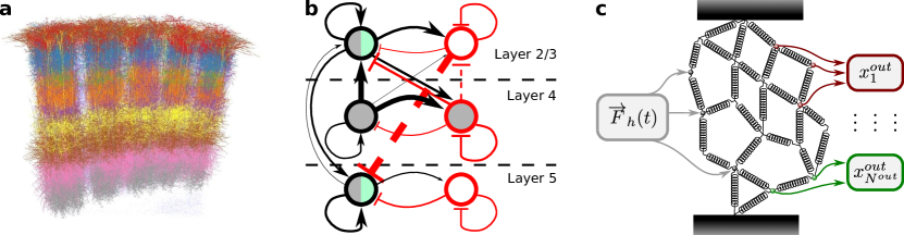
Figure 3: Reservoirs in the brain and the body. a Cortical microcolumns have been proposed as the basic operating unit of the neocortex HawkinsBlakeslee2007 . Liquid State Networks MaassMarkram2002 where largely introduced in an attempt to clarify the computational basis of these circuits. Figure credit to Oberlaender et al., reconstruction methods in OberlaenderSakmann2011 . b Schematic representation of connections between layers within a single cortical microcolumn. Figure reconstructed from HaeuslerMaass2006 ; HabenschussMaass2013 ; Maass2016 . Black node contour and black arrows represent respectively excitatory neurons and connections, red indicates inhibitory ones. Arrow width is proportional to connection strength as estimated from empirical data. Dashed arrows indicate data is less significative. Gray-filled nodes indicate they receive input from other areas – mostly cortex and thalamus. Green-filled nodes indicate they act as output – mostly to other cortical areas (both output nodes) and thalamus (layer $5$ output node). c Networks of springs can work very efficiently as reservoirs, as long as they display heterogeneous dynamics as a response to inputs. This opens a huge potential in robotics and elsewhere, since multiple mechanoelastical systems can be modeled as networked spring-mass structures.

When conceiving Liquid State Machines, Maass et al. drew inspiration from the cortical microcolumn (figure 3a). Through RC, they proposed a plausible computing strategy that could be the basic operating principle of these circuits MaassMarkram2002 ; MaassMarkram2004a ; MaassMarkram2004b ; MaassMarkram2006 . These neural motifs are roughly cylindrical structures that convey information mostly inwards from and perpendicularly to the neocortex surface. Contiguous columns are saliently distinguished from each other, but sparse lateral connections do exist. An important part of the internal structure, as well as external connections to and from other columns and other parts of the brain (notably the thalamus), appears to be stereotypical ThomsonBannister2002 . Specific connections and circuit motifs correlate with the different cortical layers within each column (figure 3b). Maass et al. built upon this known average structure when designing realistic reservoirs. Still, columns vary morphologically and functionally throughout the cortex. Most of them can hardly be associated to exclusive functionality, while others can be linked down to specific computations. For example, the receptive field of columns in V1 in cats was early identified by Hubel and Wiesel as responding to visual gratings with specific inclination HubelWiesel1962 ; the barrel cortex in mice consists of cortical columns that have grown in size through evolution and have specialized in processing the sensory stimuli from individual whiskers DiamondAhissar2008 . It has been proposed that the cortical microcolumn constitutes the operational unit of the neocortex, and that the advanced cognitive success of mammal brains is a consequence of the exhaustive use of this versatile circuit HawkinsBlakeslee2007 . Evidence about this remains inconclusive. In any case, discerning the computational basis of cortical circuits is a relevant, open question in neuroscience to which RC can contribute greatly.

In Maass2016 , Maass notes the heterogeneity of neuron types in the brain (also within cortical columns). They display great morphological diversity, varying number of presynaptic neurons, and different physiological constituency that results in diversified time and spacial integration scales. The recursive nature of most neural circuits is also highlighted. This diversity and recursivity poses a challenge to the mostly feed-forward computing paradigms engineered into our computers, which also rely on a relative homogeneity of its components to make hardware modular and reprogramable. What could then be the computational basis of neural circuits? RC comes in to take advantage of these features, and steps forward as a likely computational foundation of the brain. Looking for empirical evidence, three hallmarks have been sought in cortical circuits that would be indicative of RC: i) Records of this morphological heterogeneity, which in turn results in the dynamical diversity proper of a reservoir. ii) Existence of parallel neurons that gather information from a same processing center (akin to a repository) and project their output into distinct areas that solve different tasks; just as RC readouts use a same reservoir without interference. iii) The ability to retrieve relevant (including highly non-linear) input features by training simple linear classifiers on neural recordings. Note that all these would constitute rather circumstantial evidence for RC since each of these features could be exploited by other computing paradigms too. As of today, this is the best that we can do as far as signs of RC in the brain goes. We review a series of studies showing such indirect evidence in the next paragraphs.

Neural heterogeneity resulting in desirable, reservoir-like properties has been reported in cortical neurons, the retina and the primary visual cortex, and in networks grown in-vitro from dissociated neurons HaeuslerMaass2006 ; BernacchiaWang2011 ; NikolicMaass2009 ; MarreBerry2015 ; DraniasVanDongen2013 ; JuVanDongen2015 . The existing diversity of neural components results in very heterogeneous dynamics Singer2013 – which can be exploited by RC-like computation. The emergence of such dynamical heterogeneity in dissociated neurons reveals that this property follows spontaneously from the wiring mechanisms. Indeed, computational studies show how input-driven Spike-Timing Dependent Plasticity can generate heterogeneous circuitry that then displays good reservoir behavior KlampflMaass2013 .

As argued above, by restricting training to the output units, RC facilitates the use of a same reservoir to solve different tasks by just plugging parallel readouts that do not interfere with each other. This principle seems to be exploited by the brain. In ChenHelmchen2013 , neurons are recorded which project from the mouse barrel cortex to other sensory and motor centers. Both kinds of neurons retrieve the same information, but they respond differently, with task specificity depending on whether further sensory processing is required or whether the motor system needs to be involved. From the RC framework, the barrel cortex would be working as a reservoir whose activity is not enough to determine which neurons will respond and how, suggesting independent wiring for each individual task based on a same, shared input.

All these works casually suggest that advanced neural structures are indeed using some of the RC principles. More compelling evidence comes from the computational analysis of neural populations as they relate to input signals. More precisely, from the ability to retrieve non-linear input features by using just linear combinations of sparse, recorded neural activity KlampflMaass2012 ; RigottiFusi2013 ; FusiRigotti2016 . In KlampflMaass2012 it is shown how sparse recordings from the primary auditory cortex of ferrets (involving just between $4$ and $10$ neurons) are enough to retrieve non-linear features of auditory stimulus in a task that involves tones that increase or decrease randomly by octaves. This information can be extracted by simple linear classifiers trained upon the recorded neural activity. This is possible because the recorded neurons (which act as a reservoir) already implement a sufficient, non-linear transformation of the input. More complicated methods (e.g. Support Vector Machines) do not show a relevant performance increase. We can parsimoniously assume that evolution would settle for simpler solutions (i.e. linear readouts) if they suffice – unless unknown selective pressures existed.

The term mixed selectivity is used in RigottiFusi2013 ; FusiRigotti2016 to underscore that neurons from the reservoir in these experiments do not respond to simple (i.e., somehow linear) features of the stimulus. Measures akin to the $r^{S}$ and $r^{G}$ introduced above are computed in RigottiFusi2013 ; FusiRigotti2016 for a set of neural recordings while monkeys perform a series of tasks. It is shown how the classification accuracy grows with the dimensionality of the space (which corresponds to larger $r^{S}$) into which the neural recordings project the input stimuli. The underlying reason is, again, that this larger $r^{S}$ allows more different binary classifiers to be allocated among the data.

The baseline story is that biological neural systems in the neocortex (and potentially other parts of the brain) exhibit all the ingredients needed to implement RC. Most importantly, a lot of meaningful information can be retrieved from real neural activity using simple linear readouts. From an evolutionary point of view, it would feel suboptimal to perform further complicated operations (specially provided that they do not improve performance KlampflMaass2012 ; RigottiFusi2013 ).

III.2 The body as a reservoir

In HauserMaass2011 , Hauser et al. implement a reservoir using two-dimensional networks of springs (figure 3c). Inputs are provided as horizontal forces that displace some springs from their resting states. Such perturbations propagate through the network similarly to activity in other reservoirs. Simple linear readouts can be trained to pick up both vertical and horizontal elongations (these would constitute the internal state $\bar{x}(t)$ of the system), and thus perform all kind of computations upon the input signals. It seems trivial that such a reservoir will work as long as the springs present a variety of elastic constants (hence providing the richness of dynamics that RC demands). But a more important conceptual point is made in HauserMaass2011 : the possibility that bodies can function as reservoirs, with springs modeling muscle fibers and other sources of mechanical tension.

A more explicit implementation is explored in NakajimaPfeifer2013a ; NakajimaPfeifer2013b where the muscles of an octopus arm are simulated and used as a reservoir. Torques at the base of the arm serve as inputs. These forces propagate along the arm, perturbing modules of coupled springs (figure 3d). A simple linear classifier reads the elongation of the various springs. The readouts are trained using standard RC methods until they reproduce a desired function of the output. Alternatively, readout activity is fed back to the arm and trained so that it displays a target motion. Octopuses have a central brain with $\sim 50$ million neurons versus a distributed nervous system with $\sim 300$ million neurons NakajimaPfeifer2013a . The computational power of nerve cells along the arms is beyond doubt GodfreySmith2016 ; Sacks2017 . But this approach is telling us something much more important: a lot of the non-linear calculations needed to process and control an arm’s motion could be provided for free by spurious mechanical forces picked up by simple linear classifiers.

The non-linearities and unpredictable behavior of soft tissue could have been a nuisance in robotics. They could have been perceived as untameable systems, very costly to simulate, that a central controller would need to oversee in real time. But a recent trend termed morphological computation PfeiferBongard2006 ; PfeiferIida2007 ; MullerHoffman2017 exploits these non-linearities, self-organization, and in general the ability that soft tissues and compliant elements have shown to carry out complex computations. This framework includes simple behaviors such as passive walkers McGeer1990 ; WisseVanFrankenhuyzen2006 , materials optimized to provide sensory feedback FendPfeifer2006 , or collective self-organization of smaller robots MurataKurokawa2007 . The approach of the body as a reservoir (demonstrated by the networks of springs just described HauserMaass2011 ; NakajimaPfeifer2013a ; NakajimaPfeifer2013b ; SumiokaPfeifer2011 ; HauserMaass2012 ; NakajimaPfeifer2013c or by tensegrity structures that can crawl controlled by RC-based feedback CaluwaertsSchrauwen2011 ; CaluwaertsSchrauwen2013 ) offers a principled way to develop a sound theory of morphological computation HauserMaass2011 ; HauserMaass2012 ; MullerHoffman2017 .

Other bodily elements besides physical tensions can work as a reservoir. Recently, Gabalda-Sagarra et al. GabaldaSagarraGarciaOjalvo2018 have shown how the Gene Regulatory Network (GRN) in a range of cells (from bacteria to humans) present a structure quite suited for RC. Empirically-inspired GRNs are simulated and used as reservoirs to solve benchmark problems as good as known optimal topologies. They also show how an evolutionary process could successfully train output readouts stacked on top of those GRNs. These examples with physical bodies and gene cross-regulation highlight a potential abundance of repertoires in Nature.

They also highlight the importance of embodied computation PfeiferIida2007 ; Clark1998 – the fact that living systems develop their behavior within a physical reality whose elements (including bodies) can participate in the needed calculations, become passive processors, expand an agent’s memory, etc. In robotics, this opens up huge possibilities NakajimaPfeifer2014 ; NakajimaPfeifer2015 – e.g., to outsource much of the virtual operations needed to simulate robot bodies. From an evolutionary perspective, the powerful and affordable computations that RC offers through compliant bodies raises a series of questions. For example, with animal motor control in mind: Since RC is a valid approach to the problem, and it seems to provide so much computational power for free, why is it not more broadly used? Why would, instead, a centralized model and simulation of our body (as the one harbored by the sensory-motor areas of the cortex) become so prominent instead? What were the evolutionary forces shaping this process, which somehow displaced computation from its embodiment to favor a more virtual approach? It is still possible that, unknown to us, RC actually takes place with the body (or parts of the body) as a reservoir – after all, the paradigm has only been introduced recently (and already see ShimHusbands2007 ; ValeroCuevasLipson2007 ; MullerHoffman2017 for examples falling close enough). However, the most salient features of advanced motor control (e.g., sensory-motor cortices, the central pattern generator that regulates gait, some peripheral circuits implementing reflexes) do not resemble RC much. So the above questions can still teach us something about how RC endures different selective pressures. A possibility that we explore further in the next section is that RC shall be an unstable evolutionary solution.

IV Discussion – evolutionary paths to Reservoir Computing

RC is a very cheap and versatile paradigm. By exploiting a reservoir capable of extracting spatiotemporal, non-linear features from arbitrary input signals, simple linear classifiers suffice to solve a large collection of tasks including classification, motor control, time-series forecasting, etc VerstraetenStroobandt2006 ; JaegerSiewert2007 ; SoriaRuffini2018 ; JoshiMaass2004 ; SalmenPloger2005 ; Burgsteiner2005 ; JaegerHaas2004 ; IbanezSoriaRuffini2018 ; VerstraetenVanCampenhout2005 ; TongCottrell2007 ; TriefenbachMartens2010 ; HinautDominey2013 . This approach simplifies astonishingly the problem of training Recurrent Neural Networks, a job plagued with hard numerical and analytic difficulties BengioFrasconi1994 ; PascanuBengio2018 . Furthermore, as we have seen, reservoir-like systems abound in Nature: from non-linearities in liquids and GRNs FernandoSojakka2003 ; GabaldaSagarraGarciaOjalvo2018 , through mechanoelastic forces in muscles HauserMaass2011 ; NakajimaPfeifer2013a ; NakajimaPfeifer2013b , to the electric dynamics across neural networks MaassMarkram2002 ; MaassBertschinger2005 ; LegensteinMaass2007b ; a plethora of systems can be exploited as reservoirs. Reading off relevant, highly non-linear information from an environment becomes as simple as plugging linear perceptrons into such structures. Adopting the RC viewpoint, it appears that Nature presents a trove of meaningful information ready to be exploited and coopted by Darwinian evolution or engineers so that more complex shapes can be built and ever more intricate computations can be solved.

When looking at RC from an evolutionary perspective these advantages pose a series of questions. Where and how is RC actually employed? Why is this paradigm not as prominent as its power and simplicity would suggest? In biology, why is RC not exploited more often by living organisms (or is it?); in engineering, why is RC only so recently making a show. This section is a speculative exercise around these points. We will suggest a series of factors which, we think, are indispensable for RC to emerge and, more importantly, to persist over evolutionary time. Based on these factors we propose a key hypothesis: while RC shall emerge easily and reservoirs abound around us, these are not evolutionarily stable designs as systems specialize or scale up. If reservoirs evolve such that signals need to travel longer distances (e.g. over bigger bodies), integrate information from senses with wildly varying time scales, or carry out very specific functions (such that the generalizing properties of the reservoir are not needed anymore), then the original RC paradigm might be abandoned in favor of better options. Then, fine-tuned, dedicated circuits might evolve from the raw material that reservoirs offer. A main goal of this speculative section is to provide testable hypotheses that can be tackled computationally through simulations, thus suggesting open research questions at the interface between computation and evolution.

First of all, we should not dismiss the possibility that RC has been overlooked around us – it might actually be a frequent computing paradigm in living systems. It has only recently been introduced, which hints us that it is not as salient or intuitive as other computing approaches. There was a lot of mutual inspiration between biology and computer science as perceptrons Minsky2017 , attractor networks Hopfield1982 , or self-organized maps Kohonen1982 were introduced. Prominent systems in our brain clearly seem to use these and other known paradigms Hebb1963 ; FukushimaMiyake1982 ; YaminsDiCarlo2014 ; KhalighRazaviKriegeskorte2014 ; Ritter1990 ; SpitzerKischka1995 . We expect that RC is used as well. We have reviewed some evidence suggesting that it is exploited by several neural circuits HaeuslerMaass2006 ; BernacchiaWang2011 ; NikolicMaass2009 ; MarreBerry2015 ; DraniasVanDongen2013 ; JuVanDongen2015 ; ChenHelmchen2013 ; KlampflMaass2012 ; RigottiFusi2013 ; FusiRigotti2016 , or by body parts using the morphological computation approach ValeroCuevasLipson2007 ; ShimHusbands2007 . All this evidence, while entailing, is far from, e.g., the visually appealing similarity between the structure of the visual cortices and modern, deep convolutional neural networks for computer vision KrizhevskyHinton2012 ; YaminsDiCarlo2014 ; KhalighRazaviKriegeskorte2014 (figure 1e). Altogether, it seems fair to say that RC in biology is either scarce or elusive, even if only recently we are looking at biological systems through this optic.

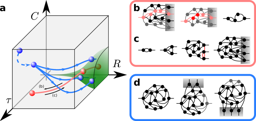
Figure 4: Evolutionary paths to and from RC. a We propose a morphospace to locate RC-based circuits (this could be extended to other computing paradigms). The axes are determined by the circuit cost ($C$), and two aspects of an underlying fitness landscape that drives circuit selection: its ruggedness ($R$) and the average lifetime ($\tau$) that computational tasks contribute to fitness. RC should ensue when both $C$ and $\tau$ are low and $R$ is high (green volume). Low $\tau$ and high $R$ demand, respectively, cheap learning and multitasking. Possible evolutionary paths of non-RC circuits into the RC area (and vice-versa) are depicted. b (Red curve in panel a.) Readout units implement simple linear classifiers (indicated by the gray rectangle). This RC-based circuit has discovered a very fit computation implemented by the red units. The other readouts and their tasks (as well as some components of the reservoir) gradually become spurious and evolutionary dynamics get rid of them. Eliminating some nodes can prompt a reorganization of the original units implementing the valuable computation (solid red units). Such a circuit migrates through the morphospace from the RC region into a position with little ruggedness and stable peaks of the landscape. The cost, too, should have been decreased. c (Also red curve in panel a, traversed in the opposite direction.) A simple circuit gradually becomes more complex. New tasks are implemented as components are appended. If true RC is reached, feedback between the outputs (marked with red links) should be lost and readout units should implement linear classifiers (again, gray rectangle). At some point, this should be noted as a certain symmetry breaking between reservoir and readout units. This might leave an empirical trace in biological systems. d (Blue trajectories in panel a.) A genetic mutation produces two copies of a very specialized circuit. One of the copies keeps implementing its very specific task (blue ball in the upper left corner of the morphospace, panel a). This represents a lasting, singled out peak in fitness landscape and the implementation is costly because mistakes would cause a fatal failure. The circuit copy is released from the cost of failure (jump represented by the blue arrow in panel a). It can then wander the morphospace freely (different blue trajectories), probably becoming cheaper as some further functionality is lost. Its very rich dynamics make it a perfect candidate to be hijacked by simple, linear readouts that start using the circuit as a reservoir.

The two main advantages brought about by RC are: i) very cheap learning and ii) a startling capability for parallel processing. Its main drawback compared to other paradigms is the amount of extra activity needed to capture incidental input features that might never be actually used. We can view these aspects of RC as evolutionary pressures defining the axes of a morphospace. Morphospaces are an insightful picture that has been used to relate instances of natural Raup1966 ; Niklas1997 ; McGhee1999 ; Niklas2004 and synthetic CorominasMurtraRodriguezCaso2013 ; AvenaKoenigsbergerSporns2015 ; SeoaneSole2018b complex systems to each other guided by metrics (sometimes rigorous, other times qualitative) that emerge from mathematical models or empirical data. Here we lean towards the qualitative side, but it should also be possible to qualitatively locate RC and other computational paradigms in the morphospace that follows. That would allow us to compare these different paradigms, or different circuit topologies within each paradigm, against each other under evolutionary pressures.

A first axis is straightforwardly the dynamical cost ($C$, figure 4a) of the reservoir, since RC demands so much more activity than it eventually uses. This would prevent RC at large organism scales with costly metabolism, but still allows myriad smaller physical systems (such as muscles or tiny bodies) to behave as free-floating reservoirs ready to be exapted.

Which brings in the next question: given these freely available reservoirs (specifically supported by the spring and gene regulatory network examples), when will they be exploited? To answer this, let us focus on the two main advantages of RC mentioned above, starting with the cheap learning. Let us also assume that there exists an underlying fitness landscape that tells us whether a feature (e.g. solving a specific computation) contributes to the success of a living organism. We conceive learning as a process much faster than evolutionary dynamics. Looking at the fitness landscape, we would expect features that offer fitness over long evolutionary periods to be hard-wired, not learned. We would not need a reservoir to capture these; but rather a robust, efficient, and dedicated structure fixed by evolution. Features which are rather learned, on the other hand, shall offer fitness on a time-scale briefer than a lifetime. We are talking about short-lived peaks of the landscape, so voluble or unpredictable that it becomes preferable to keep a learning engine rather than hardwiring a fixed design. Some notion of an average lifetime ($\tau$, figure 4a), during which a feature contributes to fitness, defines a second axis of our morphospace.

Similarly, to exploit the parallel processing abilities of RC, the underlying fitness landscape should be peaked with multiple optima that represent different useful computations. Thus ruggedness ($R$, figure 4a) defines the last axis of our morphospace. If one or few tasks contribute much more fitness than others, parts of the reservoir dedicated to them would be reinforced over evolutionary times and unimportant components would fade away, eventually thinning down the reservoir and dismissing the less fit computations (figure 4b). Over very short time-scales, the ruggedness and peak lifetime axes shall become indistinguishable: a quickly shifting single peak reminds a rugged landscape when looked at from afar.

These wildly speculative hypotheses suggest a research program amid evolution and computation. We can craft artificial fitness landscapes with computing tasks at their peaks. We could then mutate and select reservoirs with costs associated to their dynamics, and with a reward collected as they solve tasks around the shifting landscape. We expect RC to fade away if some of the conditions are removed. For example, if a reservoir grows in physical size so that communicating dynamical states over long distances becomes metabolically costly. Might this have happened in motor control for larger bodies? How would be the interplay between the advantages afforded by RC and a growing morphology? What would be the evolutionary fate of the components of a reservoir? Under what conditions do reservoirs retain their full original architecture with redundant dynamics? When do they thin down to a subset of dedicated parts that capture specific signals ignoring the rest (figure 4b)? Could some conditions prompt the development of more complex reservoirs? Can we observe a reservoir complexity ratchet – a threshold beyond which RC becomes evolutionary robust? These are all issues that can be tackled through simulations in a systematic and easy manner. Also, these questions extend beyond RC. We used its properties as guidelines to design morphospace axes that, we think, could optimally tell apart this computing strategies from others. But both the lifetime and ruggedness of tasks in our landscape are independent of the strategy used to tackle each problem. A dynamical cost can also be calculated in other computing devices. Hence, we expect that the morphospace will be useful in locating RC among a larger family of RNN and other paradigms. The eventual picture could contain hybrids as well, thus potentially revealing a continuous of computing options.

Back to RC, up to this point we have assumed that a full-fledged reservoir exists which, depending on external constraints, might shift to simpler computing paradigms and lose part of its structure (figure 4b). This shall be relevant for the kind of reservoirs provided for free by Nature, as discussed above. But there are alternative questions at the other end of the spectrum: What would be plausible evolutionary paths for non-RC circuits to progress towards RC? If cortical microcolumns actually implement RC in our brains, we could then wonder how they got there by building upon non-RC elements. Some non-exhaustive possibilities include:

• Gradually, over evolutionary time, a small, specialized circuit acquires more tasks at the same time that it becomes more complex – e.g. by incorporating more parts and a more convoluted topology (figure 4c). For this to result in RC, partial computations needed for the acquired tasks must be distributed over (somehow involving) several circuit components in a way that makes them difficult to disentangle. Otherwise, the system would more likely evolve into smaller, separate, and task- specific structures. Importantly, at some point, a kind of symmetry-breaking between the reservoir and the readouts should take place. All the costly, non-linear calculations should be relegated to the parts that will constitute the reservoir. Readouts or circuit effectors, on the other hand, can become simpler – with linear classifiers eventually sufficing to do the job. Given the way how learning works in RC, which only affects the readouts, this symmetry breaking between parts should also be reflected by a specialization of feedbacks controlling synaptic plasticity – a point that we will discuss again below.

• An already complex, yet specialized circuit is freed of its main task, thus becoming raw material that can be coopted to solve other computations (figure 4d). This evolutionary path to RC could be explored, e.g., if a complex circuit gets duplicated and one of the copies keeps implementing the original task – so that outlandish explorations are not penalized. This is a mechanism exploited elsewhere in biology, e.g., by duplicated genes with one of the copies exploring the phenotypic neighborhood of an existing peak in fitness landscape. (Indeed, we could look at such pools of duplicated genes as a reservoir of sorts; and we could wonder whether the structure, variability, and frequency of such gene reservoirs could help us quantify aspects of our RC morphospace.) The similarities between Central Pattern Generators in the brain stem and columns in the neocortex have been noted at several levels including dynamical, histological, biomolecular, patological, and structural YusteLansner2005 . A key difference is the versatility and plasticity of microcolumns when compared with the sterotypical behavior of CPGs (a versatility that would be very costly for CPGs, since they would fail to implement their main task). RC is explicitly suggested in YusteLansner2005 as a paradigm to frame the differences between CPGs and cortical columns. The hypothesis that microcolumns shall have followed this path to RC from a shared evolutionary origin with CPGs becomes tempting.

These paths to RC, again, work as evolutionary-computational hypotheses that can be easily tested through simulations. It is perhaps also possible to derive some mean-field models of average circuit structure and their computational power and address some limit cases analytically. These are all engaging topics for the future, but a look at the foundation of our speculations already offers hints to answer some of the questions above – notably, why is RC not a more prominent paradigm.

While circuits and complex systems with the ability to work as reservoirs abound in Nature, situations that sustain evolutionary pressures with a rugged, sifting landscape (demanding multitasking and adaptability within times much shorter than the lifetime of the reservoir) might not be as common. A possibility is that a peak of the fitness landscape becomes more prominent for an evolving species – e.g., by a process of niche construction. Then, a single task among the several ones solved by a reservoir can provide enough fitness. Redundant tasks and components can be consequently lost (figure 4b). As suggested in the previous section, against the convenience of bodies as a reservoir, we propose that this might be a reason why nerves at large evolved towards a more sequential and archetypal wiring. As bodies grew bigger, peaks in the motor-control landscape might have become more prominent (e.g., just a few coarse-grained commands seem enough for CPGs to coordinate gait behavior at large MarderCalabrese1996 ; Ijspeert2008 ). Even though bodies as reservoirs still serve the information needed to solve motor control, the archetypal circuitry is more stable in the long run. The need to integrate visual cues (which can hardly be incorporated into a mechanoelastic reservoir) and long-term movement planning hint at yet other evolutionary pressures against the RC solution. This suggests that smaller or more primitive organisms, if any, shall exploit RC more clearly. Just as RC appears as a relevant tool to develop a principled theory of morphological computation HauserMaass2011 ; HauserMaass2012 ; MullerHoffman2017 , it also seems a great addition to think about Liquid and Solid Brains along the lines of this volume, especially as embodied and non-standard computations with small living organisms are explored BaluskaLevin2016 .

Cortical microcolumns, on the other hand, are likely to operate based on RC or to incorporate most RC principles. These are the circuits on top of the more abstract and complex tasks, such as language or conscious processing. These tasks appear indeed shifting in nature, and often presenting a wide variety of solutions (e.g. as indicated by the different syntax and grammars that implement language equally well). These features loosely correspond to rugged landscape whose peaks either shift in time or cannot be anticipated from the long evolutionary perspective – thus fitting nicely in our speculation. Efforts to clarify whether RC is actually exploited in the neocortex and other neural circuits is underway, as reviewed earlier HaeuslerMaass2006 ; BernacchiaWang2011 ; NikolicMaass2009 ; MarreBerry2015 ; DraniasVanDongen2013 ; JuVanDongen2015 ; ChenHelmchen2013 ; KlampflMaass2012 ; RigottiFusi2013 ; FusiRigotti2016 . These works focus mostly on the richness of the dynamics and on the ability of simple linear classifiers to pick up non-linear input features based on recorded neural activity alone.

We would like to add an alternative empirical approach: As mentioned above, RC implies that training focuses on the linear readouts. This must be reflected at several levels. As an instance, the target behavior must be made available to the readouts (e.g., to implement back propagation or Hebbian learning), but is not needed elsewhere. On the other hand, we have explored a series of computation-theoretical features that reservoirs should preferably display. These include a tendency to criticality and a simultaneous maximization of the separability and generalization properties (as measured by $r^{S}$ and $r^{G}$). All these pose diverging evolutionary targets for reservoir and readout plasticity. This should result in differences in the mechanisms guiding neural wiring – perhaps even at the molecular level. Trying to spot such differences empirically should be within the reach of current technology.

We close with a reflection to link this paper with the general issue of this volume. In the introduction we anticipated that most authors would be exploring liquid or solid brains as referred to the thermodynamic state of the physical substrate in which computation happens – i.e. whether computing units are motile (ants, T-cells, …) or fixed (neurons, semiconductors, …). Instead, this paper rather tackled aspects of the software. RC largely resembles a liquid in the signals involved (sometimes literally so FernandoSojakka2003 ), specially through the abundance of spurious dynamics elicited. Evolutionary costs could limit these generous dynamics so that RC is lost (e.g., figure 4b). This could somehow crystallize the available liquid signals to a handful of stereotypical patterns. This could, in turn, either lower the demands on the hardware (as it requires less active dynamics), and otherwise free resources that could be invested, e.g., in hardware motility. We expect non-trivial interplays between afforded liquidity at the software and hardware levels. It then becomes relevant to determine whether and how the evolutionary pressures discussed above can constrain the liquid or solid nature of brain substrates, not only of its signal repertoire.

Competing interests

We declare no competing interests.

Funding

This work has been supported by the Botín Foundation, by Banco Santander through its Santander Universities Global Division, a MINECO FIS2015-67616 fellowship, and the Secretaria d’Universitats i Recerca del Departament d’Economia i Coneixement de la Generalitat de Catalunya.

References

- (1) Szathmáry E, Maynard-Smith J. 1997 From replicators to reproducers: the first major transitions leading to life. J. Theor. Biol. 187, 555-571.
- (2) Joyce GF. 2002 Molecular evolution: booting up life. Nature 420(6913), 278.
- (3) Walker SI, Davies PC. 2013 The algorithmic origins of life. J. R. Soc. Interface 10(79), 20120869.
- (4) Schuster P. 1996 How does complexity arise in evolution: Nature’s recipe for mastering scarcity, abundance, and unpredictability. Complexity 2(1), 22-30.
- (5) Smith JM. 2000 The concept of information in biology. Philos. Sci. 67(2), 177-194.
- (6) Jablonka E, Lamb MJ. 2006 The evolution of information in the major transitions. J. Theor. Biol. 239, 236-246.
- (7) Nurse P. 2008 Life, logic and information. Nature 454(7203), p.424.
- (8) Joyce GF. 2012 Bit by bit: the Darwinian basis of life. PLoS Biol. 10(5), e1001323.
- (9) Adami C. 2012 The use of information theory in evolutionary biology. Ann. NY Acad. Sci. 1256(1), 49-65.
- (10) Hidalgo J, Grilli J, Suweis S, Muñoz MA, Banavar JR and Maritan A. 2014 Information-based fitness and the emergence of criticality in living systems. Proc. Nat. Acad. Sci. 111(28), 10095-10100.
- (11) Smith E, Morowitz HJ. 2016 The origin and nature of life on Earth: the emergence of the fourth geosphere. Cambridge University Press.
- (12) Hopfield, JJ. 1994 Physics, computation, and why biology looks so different. J. Theor. Biol. 171(1), 53-60.
- (13) Jacob F. 1998 Of flies, mice and man. Harvard, MA: Harvard University Press.
- (14) Wagensberg J. 2000 Complexity versus uncertainty: the question of staying alive. Biol. Phil. 15, 493-508.
- (15) Seoane LF, Solé R. 2018 Information theory, predictability and the emergence of complex life. Roy. Soc. Open Sci. 5(2), 172221.
- (16) Paun G, Rozenberg G, Salomaa A. 2005 DNA computing: new computing paradigms. Springer Science & Business Media.
- (17) Doudna JA, Sternberg SH. 2017 A crack in creation: Gene editing and the unthinkable power to control evolution. Houghton Mifflin Harcourt.
- (18) Thomas R. 1973 Boolean formalization of genetic control circuits. J. Theor. Biol. 42(3), 563-585.
- (19) Kauffman S. 1996 At home in the universe: The search for the laws of self-organization and complexity. Oxford university press.
- (20) Rodríguez-Caso C, Corominas-Murtra B, Solé R. 2009 On the basic computational structure of gene regulatory networks. Mol. Biosyst. 5(12), 1617-1629.
- (21) Dayan P, Abbott LF. 2001 Theoretical neuroscience. Cambridge, MA: MIT Press.
- (22) Seung S. 2012 Connectome: How the brain’s wiring makes us who we are. HMH.
- (23) Levick WR. 1967 Receptive fields and trigger features of ganglion cells in the visual streak of the rabbit’s retina. J. Physiol. 188(3), 285-307.
- (24) Russell TL, Werblin FS. 2010 Retinal synaptic pathways underlying the response of the rabbit local edge detector. J. Neurophysiol. 103(5), 2757-2769.
- (25) Marr D, Hildreth E. 1980 Theory of edge detection. Proc. R. Soc. Lond. B 207(1167), 187-217.
- (26) Marr D. 1982 Vision: A computational investigation into the human representation and processing of visual information. MIT Press. Cambridge, Massachusetts.
- (27) Stephens GJ, Mora T, Tkačik G and Bialek W. 2013 Statistical thermodynamics of natural images. Phys. Rev. Let. 110(1), 018701.
- (28) Fukushima K, Miyake S. 1982 Neocognitron: A self-organizing neural network model for a mechanism of visual pattern recognition. In Competition and cooperation in neural nets (pp. 267-285). Springer, Berlin, Heidelberg.
- (29) Krizhevsky A, Sutskever I, Hinton GE. 2012 Imagenet classification with deep convolutional neural networks. In Advances in neural information processing systems, 1097-1105.
- (30) Yamins DL, Hong H, Cadieu CF, Solomon EA, Seibert D, DiCarlo JJ. 2014 Performance-optimized hierarchical models predict neural responses in higher visual cortex. Proc. Nat. Acad. Sci. 111(23), 8619-8624.
- (31) Khaligh-Razavi SM, Kriegeskorte N. 2014 Deep supervised, but not unsupervised, models may explain IT cortical representation. PLoS Comp. Biol. 10(11), e1003915.
- (32) Jaeger H. 2001 The “echo state” approach to analysing and training recurrent neural networks-with an erratum note. Bonn, Germany: German National Research Center for Information Technology GMD Technical Report, 148(34), 13.
- (33) Maass W, Natschläger T, Markram H. 2002 Real-time computing without stable states: A new framework for neural computation based on perturbations. Neural Comput. 14(11), 2531-2560.
- (34) Jaeger H, Maass W, Principe J. 2007 Special issue on echo state networks and liquid state machines. Neural Networks 20(3).
- (35) Verstraeten D, Schrauwen B, d’Haene M, Stroobandt D. 2007 An experimental unification of reservoir computing methods. Neural networks 20(3), 391-403.
- (36) Lukoševičius M, Jaeger H, Schrauwen B. 2012 Reservoir computing trends. KI-Künstliche Intelligenz 26(4), 365-371.
- (37) Rumelhart DE, Hinton GE, Williams RJ. 1986 Learning representations by back-propagating errors. Nature 323(6088), p.533.
- (38) Bengio Y, Simard P, Frasconi P. 1994 Learning long-term dependencies with gradient descent is difficult. IEEE T Neural Networks 5(2), 157-166.
- (39) Pascanu R, Mikolov T, Bengio Y. 2013 On the difficulty of training recurrent neural networks. In International Conference on Machine Learning, 1310-1318.
- (40) Verstraeten D, Schrauwen B, Stroobandt D. 2006 Reservoir-based techniques for speech recognition. In The 2006 IEEE International Joint Conference on Neural Network Proceedings (1050-1053). IEEE.
- (41) Jaeger H, Lukoševičius M, Popovici D, Siewert U. 2007 Optimization and applications of echo state networks with leaky-integrator neurons. Neural Networks 20(3), 335-352.
- (42) Soria DI, Soria-Frisch A, García-Ojalvo J, Picardo J, García-Banda G, Servera M and Ruffini G. 2018 Hypoarousal non-stationary ADHD biomarker based on echo-state networks. bioRxiv, p.271858.
- (43) Joshi P, Maass W. 2004 Movement generation and control with generic neural microcircuits. In: Biologically inspired approaches to advanced information technology (Ijspeert A, Murata A, Wakamiya N, eds) 258-273. Berlin: Springer.
- (44) Salmen M, Ploger PG. 2005 Echo state networks used for motor control. In Robotics and Automation, 2005. ICRA 2005. Proceedings of the 2005 IEEE International Conference on (1953-1958). IEEE.
- (45) Burgsteiner H. 2005 Training networks of biological realistic spiking neurons for real-time robot control. In Proceedings of the 9th international conference on engineering applications of neural networks, Lille, France (pp. 129-136).
- (46) Jaeger H, Haas H. 2004 Harnessing nonlinearity: Predicting chaotic systems and saving energy in wireless communication. Science 304(5667), 78-80.
- (47) Ibáñez-Soria D, García-Ojalvo J, Soria-Frisch A, Ruffini G. 2018 Detection of generalized synchronization using echo state networks. Chaos 28(3), 033118.
- (48) Verstraeten D, Schrauwen B, Stroobandt D, Van Campenhout J. 2005 Isolated word recognition with the liquid state machine: a case study. Information Processing Letters, 95(6), 521-528.
- (49) Tong MH, Bickett AD, Christiansen EM, Cottrell GW. 2007 Learning grammatical structure with echo state networks. Neural networks, 20(3), 424-432.
- (50) Triefenbach F, Jalalvand A, Schrauwen B, Martens JP. 2010 Phoneme recognition with large hierarchical reservoirs. In Advances in neural information processing systems (2307-2315).
- (51) Hinaut X, Dominey PF. 2013 Real-time parallel processing of grammatical structure in the fronto-striatal system: A recurrent network simulation study using reservoir computing. PloS one, 8(2), p.e52946.
- (52) Macia J, Sole R. 2014 How to make a synthetic multicellular computer. PLoS One 9(2), p.e81248.
- (53) Wyffels F, Schrauwen B, Stroobandt D. 2008 Stable output feedback in reservoir computing using ridge regression. In International conference on artificial neural networks (pp. 808-817). Springer, Berlin, Heidelberg.
- (54) Lukoševičius M, Jaeger H. 2009 Reservoir computing approaches to recurrent neural network training. Comput. Sci. Rev. 3(3), 127-149.
- (55) Jaeger H. 2002 Tutorial on training recurrent neural networks, covering BPPT, RTRL, EKF and the “echo state network” approach (Vol. 5). Bonn: GMD-Forschungszentrum Informationstechnik.
- (56) Lukoševičius M. 2012 A practical guide to applying echo state networks. In Neural networks: Tricks of the trade (pp. 659-686). Springer, Berlin, Heidelberg.
- (57) Maass W, Joshi P, Sontag ED. 2007 Computational aspects of feedback in neural circuits. PLoS Comput. Biol., 3(1), p.e165.
- (58) Sussillo D, Abbott LF. 2009 Generating coherent patterns of activity from chaotic neural networks. Neuron, 63(4), pp.544-557.
- (59) Dai J, Venayagamoorthy GK, Harley RG. 2009 An introduction to the echo state network and its applications in power system. In Intelligent System Applications to Power Systems, 2009. ISAP’09. 15th International Conference on (pp. 1-7). IEEE.
- (60) Rivkind A, Barak O. 2017 Local dynamics in trained recurrent neural networks. Phys. Rev. Let., 118(25), p.258101.
- (61) Ceni A, Ashwin P, Livi L. 2018 Interpreting RNN behaviour via excitable network attractors. arXiv preprint arXiv:1807.10478.
- (62) Maass W, Legenstein RA, Bertschinger N. 2005 Methods for estimating the computational power and generalization capability of neural microcircuits. In Advances in neural information processing systems, 865-872.
- (63) Legenstein R, Maass W. 2007 Edge of chaos and prediction of computational performance for neural circuit models. Neural Networks 20(3), 323-334.
- (64) Hauser H, Ijspeert AJ, Füchslin RM, Pfeifer R, Maass W. 2011 Towards a theoretical foundation for morphological computation with compliant bodies. Biol. Cybern. 105, 355-370.
- (65) Nakajima K, Hauser H, Kang R, Guglielmino E, Caldwell DG, Pfeifer R. 2013 A soft body as a reservoir: case studies in a dynamic model of octopus-inspired soft robotic arm. Front. Comput. Neurosc. 7, 91.
- (66) Nichele S, Gundersen MS. 2017 Reservoir Computing Using Non-Uniform Binary Cellular Automata. arXiv preprint arXiv:1702.03812.
- (67) Soriano MC, Ortín S, Keuninckx L, Appeltant L, Danckaert J, Pesquera L, Van der Sande G. 2015 Delay-based reservoir computing: noise effects in a combined analog and digital implementation. IEEE transactions on neural networks and learning systems, 26(2), pp.388-393.
- (68) Du C, Cai F, Zidan MA, Ma W, Lee SH, Lu WD. 2017 Reservoir computing using dynamic memristors for temporal information processing. Nat. Com. 8(1), p.2204.
- (69) Fernando C, Sojakka S. 2003 Pattern recognition in a bucket. In European conference on artificial life (pp. 588-597). Springer, Berlin, Heidelberg.
- (70) Appeltant L, Soriano MC, Van der Sande G, Danckaert J, Massar S, Dambre J, Schrauwen B, Mirasso CR, Fischer I. 2011 Information processing using a single dynamical node as complex system. Nat. Commun. 2, 468.
- (71) Paquot Y, Duport F, Smerieri A, Dambre J, Schrauwen B, Haelterman M, Massar S. 2012 Optoelectronic reservoir computing. Sci. Rep. 2, 287.
- (72) Vandoorne K, Mechet P, Van Vaerenbergh T, Fiers M, Morthier G, Verstraeten D, Schrauwen B, Dambre J, Bienstman P. 2014 Experimental demonstration of reservoir computing on a silicon photonics chip. Nat. Commun., 5, p.3541.
- (73) Legenstein R, Maass W. 2007 What makes a dynamical system computationally powerful. New directions in statistical signal processing: From systems to brain, 127-154.
- (74) Vapnik V. 1998 Statistical learning theory. Wiley, New York.
- (75) Cherkassky V, Mulier F. 1998 Learning from data: Concepts, theory, and methods. New York: Wiley.
- (76) Markram H, Wang Y, Tsodyks M. 1998 Differential signaling via the same axon of neocortical pyramidal neurons. Proc. Nat. Acad. Sci. 95(9), 5323-5328.
- (77) Coello CC. 2006 Evolutionary multi-objective optimization: a historical view of the field. IEEE computational intelligence magazine, 1(1), pp.28-36.
- (78) Schuster P. 2012 Optimization of multiple criteria: Pareto efficiency and fast heuristics should be more popular than they are. Complexity, 18(2), pp.5-7.
- (79) Seoane LF. 2016 Multiobjetive optimization in models of synthetic and natural living systems. PhD Thesis, Universitat Pompeu Fabra.
- (80) Shoval O, Sheftel H, Shinar G, Hart Y, Ramote O, Mayo A, Dekel E, Kavanagh K, Alon U. 2012 Evolutionary trade-offs, Pareto optimality, and the geometry of phenotype space. Science, p.1217405.
- (81) Hart Y, Sheftel H, Hausser J, Szekely P, Ben-Moshe NB, Korem Y, Tendler A, Mayo AE, Alon U. 2015 Inferring biological tasks using Pareto analysis of high-dimensional data. Nat. Methods, 12(3), p.233.
- (82) Szekely P, Korem Y, Moran U, Mayo A, Alon U. 2015 The mass-longevity triangle: Pareto optimality and the geometry of life-history trait space. PLoS Comp. Biol., 11(10), p.e1004524.
- (83) Tendler A, Mayo A, Alon U. 2015 Evolutionary tradeoffs, Pareto optimality and the morphology of ammonite shells. BMC Syst. Biol., 9(1), p.12.
- (84) Seoane LF, Solé R. 2013 A multiobjective optimization approach to statistical mechanics. arXiv preprint arXiv:1310.6372.
- (85) Seoane LF, Solé’ R. 2015 Phase transitions in Pareto optimal complex networks. Physical Review E, 92(3), p.032807.
- (86) Seoane LF, Solé R. 2016 Multiobjective optimization and phase transitions. In Proceedings of ECCS 2014 (pp. 259-270). Springer, Cham.
- (87) Seoane LF, Solé’ R. 2015 Systems poised to criticality through Pareto selective forces. arXiv preprint arXiv:1510.08697.
- (88) Bak P. 1996 How nature works: the science of self-organized criticality. Springer Science & Business Media.
- (89) Beggs JM, Plenz D. 2003 Neuronal avalanches in neocortical circuits. J. Neurosci., 23(35), pp.11167-11177.
- (90) Chialvo DR. 2010 Emergent complex neural dynamics. Nat. Phys., 6(10), p.744.
- (91) Mora T, Bialek W. 2011 Are biological systems poised at criticality?. J. Stat. Phys., 144(2), pp.268-302.
- (92) Tagliazucchi E, Balenzuela P, Fraiman D, Chialvo DR. 2012 Criticality in large-scale brain fMRI dynamics unveiled by a novel point process analysis. Front. Physiol., 3, p.15.
- (93) Moretti P, Muñoz MA. 2013 Griffiths phases and the stretching of criticality in brain networks. Nat. Com., 4, 2521.
- (94) Munoz MA. 2018 Colloquium: Criticality and dynamical scaling in living systems. Rev. Mod. Phys., 90(3), 031001.
- (95) Wolfram S. 1984 Universality and complexity in cellular automata. Physica D, 10(1-2), 1-35.
- (96) Langton CG. 1990 Computation at the edge of chaos: phase transitions and emergent computation. Physica D, 42(1-3), 12-37.
- (97) Mitchell M, Hraber P, Crutchfield JP. 1993 Revisiting the edge of chaos: Evolving cellular automata to perform computations. arXiv preprint adap-org/9303003.
- (98) Bertschinger N, Natschläger T. 2004 Real-time computation at the edge of chaos in recurrent neural networks. Neural Computation, 16(7), 1413-1436.
- (99) Schrauwen B, Büsing L, Legenstein RA. 2009 On computational power and the order-chaos phase transition in reservoir computing. In Advances in Neural Information Processing Systems (pp. 1425-1432).
- (100) Toyoizumi T, Abbott LF. 2011 Beyond the edge of chaos: Amplification and temporal integration by recurrent networks in the chaotic regime. Physical Review E, 84(5), 051908.
- (101) Boedecker J, Obst O, Lizier JT, Mayer NM, Asada M. 2012 Information processing in echo state networks at the edge of chaos. Theory in Biosciences, 131(3), pp.205-213.
- (102) Bianchi FM, Livi L, Alippi C. 2018 Investigating echo-state networks dynamics by means of recurrence analysis. IEEE transactions on neural networks and learning systems, 29(2), pp.427-439.
- (103) Bianchi FM, Livi L, Alippi C. 2018 On the Interpretation and Characterization of Echo State Networks Dynamics: A Complex Systems Perspective. In Advances in Data Analysis with Computational Intelligence Methods (pp. 143-167). Springer, Cham.
- (104) Livi L, Bianchi FM, Alippi C. 2018 Determination of the edge of criticality in echo state networks through Fisher information maximization. IEEE Transactions on Neural Networks and Learning Systems, 29(3), pp.706-717.
- (105) Prokopenko M, Lizier JT, Obst O, Wang XR. 2011 Relating Fisher information to order parameters. Phys. Rev. E, 84(4), 041116.
- (106) Maass W, Natschläger T and Markram H. 2004 Computational models for generic cortical microcircuits. Comp. Neurosci., 18, p.575.
- (107) Maass W, Natschläger T, Markram H. 2004 Fading memory and kernel properties of generic cortical microcircuit models. J. Physiol.-Paris, 98(4-6), pp.315-330.
- (108) Maass W, Markram H. 2006 Theory of the computational function of microcircuit dynamics. In The interface between neurons and global brain function, Dahlem Workshop Report (Vol. 93, pp. 371-390).
- (109) Thomson AM, West DC, Wang Y, Bannister AP. 2002 Synaptic connections and small circuits involving excitatory and inhibitory neurons in layers 2-5 of adult rat and cat neocortex: triple intracellular recordings and biocytin labelling in vitro. Cerebral cortex, 12(9), pp.936-953.
- (110) Hubel DH, Wiesel TN. 1962 Receptive fields, binocular interaction and functional architecture in the cat’s visual cortex. J. Physiol., 160(1), 106-154.
- (111) Diamond ME, Von Heimendahl M, Knutsen PM, Kleinfeld D, Ahissar E. 2008 ‘Where’ and ‘what’ in the whisker sensorimotor system. Nat. Rev. Neurosci., 9(8), 601.
- (112) Hawkins J, Blakeslee S. 2007 On intelligence: How a new understanding of the brain will lead to the creation of truly intelligent machines. Macmillan.
- (113) Oberlaender M, de Kock CP, Bruno RM, Ramirez A, Meyer HS, Dercksen VJ, Helmstaedter M, Sakmann B. 2011 Cell type-specific three-dimensional structure of thalamocortical circuits in a column of rat vibrissal cortex. Cereb. Cortex 22(10), pp.2375-2391.
- (114) Habenschuss S, Jonke Z, Maass W. 2013 Stochastic computations in cortical microcircuit models. PLoS Comp Biol 9(11), p.e1003311.
- (115) Haeusler S, Maass W. 2006 A statistical analysis of information-processing properties of lamina-specific cortical microcircuit models. Cereb. Cortex 17(1), pp.149-162.
- (116) Maass W. 2016 Searching for principles of brain computation. Current Opinion in Behavioral Sciences, 11, 81-92.
- (117) Bernacchia A, Seo H, Lee D, Wang XJ. 2011 A reservoir of time constants for memory traces in cortical neurons. Nat. Neurosci., 14(3), 366.
- (118) Nikolić D, Häusler S, Singer W, Maass W. 2009 Distributed fading memory for stimulus properties in the primary visual cortex. PLoS Biol., 7(12), p.e1000260.
- (119) Dranias MR, Ju H, Rajaram E, VanDongen AM. 2013 Short-term memory in networks of dissociated cortical neurons. J. Neurosci., 33(5), pp.1940-1953.
- (120) Ju H, Dranias MR, Banumurthy G, VanDongen, AM. 2015 Spatiotemporal memory is an intrinsic property of networks of dissociated cortical neurons. J. Neurosci., 35(9), 4040-4051.
- (121) Marre O, Botella-Soler V, Simmons KD, Mora T, Tkačik G, Berry II MJ. 2015 High accuracy decoding of dynamical motion from a large retinal population. PLoS Comp. Biol., 11(7), p.e1004304.
- (122) Singer W. 2013 Cortical dynamics revisited. Trends in cognitive sciences, 17(12), 616-626.
- (123) Klampfl S, Maass W. 2013 Emergence of dynamic memory traces in cortical microcircuit models through STDP. J. Neurosci., 33(28), 11515-11529.
- (124) Chen JL, Carta S, Soldado-Magraner J, Schneider BL, Helmchen F. 2013 Behaviour-dependent recruitment of long-range projection neurons in somatosensory cortex. Nature, 499(7458), 336.
- (125) Klampfl S, David SV, Yin P, Shamma SA, Maass W. 2012 A quantitative analysis of information about past and present stimuli encoded by spikes of A1 neurons. J. Neurophysiol., 108(5), 1366-1380.
- (126) Rigotti M, Barak O, Warden MR, Wang XJ, Daw ND, Miller EK, Fusi S. 2013 The importance of mixed selectivity in complex cognitive tasks. Nature, 497(7451), 585.
- (127) Fusi S, Miller EK, Rigotti M. 2016 Why neurons mix: high dimensionality for higher cognition. Current opinion in neurobiology, 37, 66-74.
- (128) Nakajima K, Hauser H, Kang R, Guglielmino E, Caldwell DG, Pfeifer R. 2013 Computing with a muscular-hydrostat system. In Robotics and Automation (ICRA), 2013 IEEE International Conference on (pp. 1504-1511). IEEE.
- (129) Godfrey-Smith P. 2016 Other minds: The octopus, the sea, and the deep origins of consciousness. Farrar, Straus and Giroux.
- (130) Sacks O. 2017 The river of consciousness, Ch. 3. Picador.
- (131) Pfeifer R, Bongard J. 2006 How the body shapes the way we think: a new view of intelligence. MIT press.
- (132) Pfeifer R, Lungarella M, Iida F. 2007 Self-organization, embodiment, and biologically inspired robotics. Science 318(5853), 1088-1093.
- (133) Müller VC, Hoffmann M. 2017 What is morphological computation? On how the body contributes to cognition and control. Artif. Life 23(1), 1-24.
- (134) McGeer T. 1990 Passive dynamic walking. I. J. Robotic Res. 9(2), 62-82.
- (135) Wisse M, Van Frankenhuyzen J. 2006 Design and construction of MIKE; a 2-D autonomous biped based on passive dynamic walking. In Adaptive motion of animals and machines (pp. 143-154). Springer, Tokyo.
- (136) Fend M, Bovet S, Pfeifer R. 2006 On the influence of morphology of tactile sensors for behavior and control. Robot. Auton. Syst., 54(8), 686-695.
- (137) Murata S, Kurokawa H. 2007 Self-reconfigurable robots. IEEE Robot. Autom. Mag., 14(1), 71-78.
- (138) Hauser H, Ijspeert AJ, Füchslin RM, Pfeifer R, Maass W. 2012 The role of feedback in morphological computation with compliant bodies. Biol. Cybern. 106(10), 595-613.
- (139) Sumioka H, Hauser H, Pfeifer R. 2011 Computation with mechanically coupled springs for compliant robots. In Intelligent Robots and Systems (IROS), 2011 IEEE/RSJ International Conference on (pp. 4168-4173). IEEE.
- (140) Nakajima K, Hauser H, Kang R, Guglielmino E, Caldwell DG, Pfeifer R. 2013 Computing with a muscular-hydrostat system. In Robotics and Automation (ICRA), 2013 IEEE International Conference on (pp. 1504-1511). IEEE.
- (141) Caluwaerts K, Schrauwen B. 2011 The body as a reservoir: locomotion and sensing with linear feedback. In 2nd International conference on Morphological Computation (ICMC 2011).
- (142) Caluwaerts K, D’Haene M, Verstraeten D, Schrauwen B. 2013 Locomotion without a brain: physical reservoir computing in tensegrity structures. Artif. Life 19(1), 35-66.
- (143) Gabalda-Sagarra M, Carey LB, García-Ojalvo J. 2018 Recurrence-based information processing in gene regulatory networks. Chaos 28(10), p.106313.
- (144) Clark A. 1998 Being there: Putting brain, body, and world together again. MIT press.
- (145) Nakajima K, Li T, Hauser H, Pfeifer R. 2014 Exploiting short-term memory in soft body dynamics as a computational resource. J. R. Soc. Interface, 11(100), 20140437.
- (146) Nakajima K, Hauser H, Li T, Pfeifer R. 2015 Information processing via physical soft body. Sci. Rep., 5, 10487.
- (147) Shim Y, Husbands P. 2007 Feathered flyer: integrating morphological computation and sensory reflexes into a physically simulated flapping-wing robot for robust flight manoeuvre. In European Conference on Artificial Life (pp. 756-765). Springer, Berlin, Heidelberg.
- (148) Valero-Cuevas FJ, Yi JW, Brown D, McNamara RV, Paul C, Lipson H. 2007 The tendon network of the fingers performs anatomical computation at a macroscopic scale. IEEE T. Bio-Med. Eng. 54(6), 1161-1166.
- (149) Minsky M, Papert SA. 2017 Perceptrons: An introduction to computational geometry. MIT press.
- (150) Hopfield JJ. 1982 Neural networks and physical systems with emergent collective computational abilities. Proc. Nat. Acad. Sci. 79(8), 2554-2558.
- (151) Kohonen T. 1982 Self-organized formation of topologically correct feature maps. Biol. Cybern. 43(1), 59-69.
- (152) Hebb DO. 1963 The Organizations of Behavior: a Neuropsychological Theory. Lawrence Erlbaum.
- (153) Ritter H. 1990 Self-organizing maps for internal representations. Psychol. Res., 52(2-3), 128-136.
- (154) Spitzer M, Bhöler P, Weisbrod M, Kischka U. 1995 A neural network model of phantom limbs. Biol. Cybern., 72(3), pp.197-206.
- (155) Raup DM. 1966 Geometric analysis of shell coiling: general problems. Journal of Paleontology, pp.1178-1190.
- (156) Niklas KJ. 1997 The evolutionary biology of plants. Chicago U. Press.
- (157) McGhee GR. 1999 Theoretical morphology: the concept and its applications. Columbia U. Press.
- (158) Niklas KJ. 2004 Computer models of early land plant evolution. Annu. Rev. Earth Planet. Sci., 32, 47-66.
- (159) Corominas-Murtra B, Goñi J, Solé RV and Rodríguez-Caso C. 2013 On the origins of hierarchy in complex networks. Proc. Nat. Acad. Sci., 110(33), 13316-13321.
- (160) Avena-Koenigsberger A, Goñi J, Solé R and Sporns O. 2015 Network morphospace. J. R. Soc. Interface, 12(103), 20140881.
- (161) Seoane LF, Solé R. 2018 The morphospace of language networks. Sci. Rep., 8, 10465.
- (162) Yuste R, MacLean JN, Smith J, Lansner A. 2005 The cortex as a central pattern generator. Nat. Rev. Neurosci. 6(6), 477-483.
- (163) Marder E, Calabrese RL. 1996 Principles of rhythmic motor pattern generation. Physiol. Rev., 76(3), 687-717.
- (164) Ijspeert AJ. 2008 Central pattern generators for locomotion control in animals and robots: a review. Neural Networks, 21(4), 642-653.
- (165) Baluška F, Levin M. 2016 On having no head: cognition throughout biological systems. Front. Psychol., 7, p.902.