Embedding black holes and other inhomogeneities in the universe in various theories of gravity: a short review
The classic black hole mechanics and thermodynamics are formulated for stationary black holes with event horizons. Alternative theories of gravity of interest for cosmology contain a built-in time-dependent cosmological “constant” and black holes are not stationary. Realistic black holes are anyway dynamical because they interact with astrophysical environments or, at a more fundamental level, because of backreaction by Hawking radiation. In these situations the teleological concept of event horizon fails and apparent or trapping horizons are used instead. Even as toy models, black holes embedded in cosmological “backgrounds” and other inhomogeneous universes constitute an interesting class of solutions of various theories of gravity. We discuss the known phenomenology of apparent and trapping horizons in these geometries, focusing on spherically symmetric inhomogeneous universes.
1 Introduction
Black holes are a fundamental prediction of General Relativity (GR) and have been the subject of a celebrated theory of dynamics and thermodynamics developed in the 1970s [133]. The black holes considered in these studies are stationary solutions of GR. Real black holes, however, are non-stationary due to several possible processes:
-
•
A cosmological background: real black holes are embedded in the universe and, although this feature may be irrelevant for their astrophysics, their asymptotics are quite relevant in problems of principle and in mathematical physics. Alternative theories of gravity advocated to explain the present acceleration of the universe without an ad hoc dark energy contain a built-in, time-dependent effective cosmological “constant” and black holes in these theories are asymptotically Friedmann-Lemaître-Robertson-Walker (FLRW).
- •
-
•
Hawking radiation and evaporation affect all black holes and are, therefore, important and unavoidable in all problems of principle. They become important for hypothetical small black holes in their final stages or perhaps even for primordial black holes in the early universe.
1.1 A problem of principle
The non-stationarity of black holes constitutes a problem that may be safely ignored in most astrophysical contexts but it becomes important, or even crucial, in a fundamental physics context. Let us recall a few motivations for the study of dynamical black holes (a more extensive discussion can be found in [122, 45]).
The first problem to note is the fact that black holes are embedded in a universe, that is, they are not asymptotically flat. Asymptotic flatness is an essential ingredient in the proof of the no-hair theorems of scalar-tensor gravity, which provide a fundamental understanding of black holes in these theories. While there is literature on asymptotically de Sitter or anti-de Sitter black holes, it is much more realistic to consider asymptotically FLRW black holes. In the astrophysical context, the cosmological asymptotics cannot be neglected for primordial black holes.
Theories of gravity alternative to GR, aiming at explaining the cosmic acceleration without dark energy (e.g., gravity [24, 26]) contain a built-in, time-dependent cosmological “constant”. Therefore, black holes in theories of this class which are relevant for present-day cosmology are not asymptotically flat. Understanding black holes is an important part of understanding a theory of gravity, and the FLRW asymptotics are essential here.
Dynamical inhomogeneous spherically symmetric universes are theoretical testbeds which allow one to probe ideas about the backreaction of inhomogeneities, or the idea that we live in a giant void, which have been proposed as alternatives to dark energy to explain the cosmic acceleration (see the review [19]).
Black hole mechanics and thermodynamics were developed for stationary black holes with event horizons, which are null surfaces. Realistic black holes are instead dynamical and have apparent horizons, which are timelike or spacelike surfaces and they may change their causal nature during the evolution.
If primordial black holes were formed in the early universe, at some time they could have had a size non-negligible in comparison with the Hubble scale and very dynamical horizons. A relevant question is how fast they could have accreted material and have grown, even though primordial black holes are unlikely to be a dominant component of dark matter today. Another interesting problem of principle is the accretion of dark energy, especially phantom energy, onto black holes [9, 28, 73, 39, 87, 57, 62, 125, 126, 59, 68, 8, 105, 27]. The simplest model is, of course, spherical accretion but this is already a very non-trivial problem requiring the introduction of some toy model.
Another motivation of principle is the study of the spatial variation of the fundamental constants of physics. This idea goes back to Dirac and is partially implemented in scalar-tensor gravity, in which the gravitational coupling strength becomes a dynamical field (roughly speaking, the inverse of the Brans-Dicke scalar field ). While the time variation of has been studied extensively in scalar-tensor cosmology, its spatial variation requires the analysis of inhomogeneous universes, which have been the subject of a much smaller literature.
1.2 A practical problem
There is a much more practical and urgent problem in gravitational physics: highly dynamical black holes are very important in certain astrophysical applications. The first direct detection of gravitational waves by the LIGO interferometers involved a black hole merger [1]. In the final approach and during coalescence of these black holes, the spacetime is extremely dynamical. The signal to noise ratio in LIGO interferometers is typically low and one needs to match the signal to templates calculated theoretically. Numerical simulations of black hole mergers are used to generate banks of templates of gravitational waveforms for LIGO detection. These simulations do not rely on event horizons, but they use instead apparent and trapping horizons. Event horizons are essentially useless for practical purposes such as the generation of these banks of templates. Even though an unusually loud gravitational wave signal from a binary black hole merger can be spotted without templates, the determination of the orbital parameters of the black hole binary requires fitting the signal with templates computed by using apparent horizons. In the calculations producing these templates, “black holes” are identified with outermost marginally trapped surfaces and apparent horizons (e.g., [129, 14, 29, 33]). It is fair to say that, in practice, in astrophysics we use apparent horizons and not event horizons.
It is impossible to discuss dynamical black holes without speaking of apparent horizons. Therefore, in the next section we introduce apparent and trapping horizons and their problems. Sec. 3 presents a selection of exact solutions of various theories of gravity describing black holes embedded in cosmological “backgrounds”.111We use the word “background” in quotation marks because the non-linearity of the field equations forbids splitting the spacetime metric into a background and deviations from it in a covariant way (except for algebraically special geometries such as Kerr-Schild metrics). The last section outlines open problems.
2 Apparent horizons and their problems
In the words of Rindler [113], a horizon is a frontier between things observable and things unobservable. The horizon, a product of strong gravity, characterizes a black hole.
There are several kinds of “textbook” horizons: Rindler horizons associated with uniform acceleration even in flat space, black hole horizons, and cosmological horizons. There are event, Killing, inner, outer, Cauchy, apparent, trapping, quasi-local, isolated, dynamical, and slowly evolving horizons [112, 133, 20, 96, 7, 60]. Various horizon notions coincide for stationary black holes.
In black hole thermodynamics, if the “background” is not Minkowskian, the internal energy appearing in the first law of thermodynamics must be defined carefully. This is identified with a quasi-local energy. In spherical symmetry, this is the Misner-Sharp-Hernandez energy [95, 70], to which the more general Hawking-Hayward quasilocal energy [64, 65] reduces. In spherical symmetry, the Hawking-Hayward/Misner-Sharp-Hernandez quasilocal energy is in practice closely related to the notion of apparent horizon.
Let us begin by reviewing the concepts of null geodesic congruence and trapped surface necessary to define apparent horizons [133, 112]. Consider a congruence of null geodesics, each with tangent , where is an affine parameter along the geodesic. (The assumption of an affine parameter is not mandatory, but it simplifies several of the following equations.) With affine parametrization, the tangent satisfies and . The metric in the 2-space orthogonal to is determined as follows. Pick another null vector field such that and , then
| (2.1) |
The tensor is purely spatial and is the projection operator on the 2-space orthogonal to . The choice of is not unique, but the geometric quantities of interest to us do not depend on it once is fixed [112]. Let be the geodesic deviation vector and define the tensor
| (2.2) |
orthogonal to the null geodesics. The transverse part of the deviation vector is
| (2.3) |
and the orthogonal component of , denoted by a tilde, is
| (2.4) |
Now decompose the transverse tensor as
| (2.5) |
where the expansion propagates according to the Raychaudhuri equation [133, 112]
| (2.6) |
If the null geodesic congruence is not affinely parametrized, the geodesic equation is
| (2.7) |
(where is sometimes used as a possible notion of surface gravity) and
| (2.8) |
or
| (2.9) |
The difference between Eq. (2.7) and our previous definition is due to the fact that the geodesics in Eq. (2.7) are not required to be affinely parametrized, while the definition does require an affine parameter and measures precisely the failure of geodesics to be affinely parameterized. Since arises purely from the choice of parametrization, its significance as a surface gravity is questionable and, indeed, several alternative definitions of “surface gravity” exist in the literature (see Refs. [99, 111]) for reviews).
With non-affine parametrization, the Raychaudhuri equation then becomes
| (2.10) |
A compact and orientable surface has two independent
directions orthogonal to it, corresponding to ingoing and
outgoing null geodesics with tangents and , respectively.
Let us give some basic definitions for closed 2-surfaces.
Definition: A normal surface corresponds to
and .
Definition: A trapped surface corresponds to
and .
The outgoing, in addition to the ingoing, future-directed null rays
converge here instead of diverging and outward-propagating light is
dragged back by strong gravity.
Definition: A marginally outer trapped (or
marginal) surface (MOTS)
corresponds to (where is the outgoing null normal
to the surface)
and .
Definition: An untrapped surface is one with
.
Definition: An antitrapped surface corresponds to
and .
Definition: A marginally outer trapped tube (MOTT)
is a 3-dimensional surface which can be foliated entirely by marginally
outer trapped (2-dimensional) surfaces.
A 1965 result by Penrose [110] states that if a spacetime contains a trapped surface, the null energy condition holds, and there is a non-compact Cauchy surface for the spacetime, then this spacetime contains a singularity. Timelike naked singularities are believed to be unphysical since they spoil the initial value problem and cause the loss of predictability. Therefore, black hole horizons assume a crucial role in physics, which is hiding these singularities from the world outside the horizon.
Trapped surfaces are essential features in the concept of black hole. “Horizons” of practical utility are identified with boundaries of spacetime regions containing trapped surfaces.222The mathematical conditions for the existence and uniqueness of marginally outer trapped surfaces are not completely clear.
2.1 Event horizons
Definition: An event horizon is a connected
component of the boundary of the causal past of future null infinity .
An event horizon is a causal boundary separating a region from which nothing can come out to reach a distant observer from a region in which signals can be sent out and eventually arrive to this observer. An event horizon is generated by the null geodesics which fail to reach infinity. Provided that it is smooth, an event horizon is a null hypersurface.
In order to define and locate an event horizon, one must know all the future history of spacetime: the event horizon is a globally defined concept and has teleological nature. As an example, consider a collapsing Vaidya spacetime described by the geometry [131]
| (2.11) |
where is a retarded time, is the areal radius, is the line element on the unit 2-sphere, and is a time- and radius-dependent mass function. The apparent horizon is located by the root of the equation , which yields . The apparent horizon is distinct from the event horizon, which is given approximately by the expression [10, 20, 15, 97, 137]
| (2.12) |
where . The phenomenology of the event horizons is reported in several studies (e.g., [10, 20, 15, 97, 137] and we will not repeat the analysis here. To summarize the situation, an event horizon forms and grows starting from the centre and an observer can cross it and be unaware of it even though his or her causal past consists entirely of a portion of Minkowski space. This event horizon cannot be detected by this observer with a physical experiment and it “knows” about events belonging to a spacetime region very far away and in its future, but not causally connected to it (a property called “clarvoyance”) [7, 15, 16].
Properly speaking, an event horizon is a tube in spacetime. There is some language abuse in the literature, which consists of referring to the intersections of with surfaces of constant time (which produce 2-surfaces) as “event horizons”.
2.2 Apparent and trapping horizons
Definition: A future apparent horizon is the
closure of a 3-surface which is foliated by marginal surfaces.
An apparent horizon is defined by the conditions on the time slicings [66]
| (2.13) | |||
| (2.14) |
where and are the expansions of the future-directed outgoing and ingoing null geodesic congruences, respectively, which have tangent333Correspondingly, the expansions of the outgoing and ingoing null geodesic congruences are labelled and . fields and (outgoing null rays momentarily stop expanding and turn around at the horizon). In simple words, an event horizon is a surface from the interior of which nothing will ever emerge, while an apparent horizon is a surface from the interior of which nothing can escape now. The inequality (2.14) distinguishes between black holes and white holes.
Apparent horizons are defined quasi-locally and they do not require the knowledge of the global structure of spacetime, including future null infinity. In this sense, they are much more practical entities than event horizons. However, apparent horizons have a serious limitation: they depend on the choice of the foliation of the 3-surface with marginal surfaces. This foliation-dependence is exemplified dramatically by the fact that non-symmetric slicings of the Schwarzschild spacetime exist for which there is no apparent horizon [134, 120]. In non-stationary situations, apparent horizons and event horizons do not coincide. This foliation-dependence problem is overlooked: it implies that the very existence of a dynamical black hole depends on the observer. This problem is alleviated (or, for purely practical purposes, largely eliminated), but not solved, in spherical symmetry. In this case, the apparent horizons coincide in all spherical foliations [51].
In GR, a black hole apparent horizon lies inside the event horizon
provided that the null curvature condition for
all null vectors is satisfied. However, Hawking radiation itself
violates the weak and the null energy conditions, as do quantum matter and
non-minimally coupled scalars, hence apparent horizons cannot always be
expected to lie inside event horizons in the presence of quantum fields
or in theories of gravity alternative to GR.
Definition: A future outer trapping horizon (FOTH)
is the closure of a
surface (usually a 3-surface) foliated by marginal surfaces such
that on its 2-dimensional “time slicings” [66]
| (2.15) | |||
| (2.16) | |||
| (2.17) |
The last condition distinguishes between inner and outer horizons and
between apparent and trapping horizons (the sign distinguishes between
future and past horizons).
Definition: A past inner trapping horizon (PITH) is
defined by exchanging
with and reversing the signs of the
inequalities,
| (2.18) | |||
| (2.19) | |||
| (2.20) |
The PITH identifies a white hole or a cosmological horizon. As one moves just inside an outer trapping horizon, one encounters trapped surfaces, while trapped surfaces are encountered as as one moves just outside an inner trapping horizon. As an example, consider the Reissner-Nordström black hole with the natural spherically symmetric foliation. The event horizon is a future outer trapping horizon (FOTH), the inner (Cauchy) horizon is a future inner trapping horizon (FITH), while the white hole horizons are past trapping horizons (PTHs).
Black hole trapping horizons have been associated with thermodynamics. It is claimed that it is the trapping horizon area, and not the area of the event horizon, which should be associated with entropy in black hole thermodynamics [63, 71, 32, 96]. This claim is somewhat controversial [121, 34, 98]. The Parikh-Wilczek [108] “tunneling” approach, originally applied to study Hawking radiation from stationary black holes, is in principle applicable also to apparent and trapping horizons.
2.3 Spherical symmetry
As usual, assuming a symmetry greatly simplifies a physical problem, and this is even more so for the assumption of spherical symmetry when discussing apparent horizons and dynamical black holes. The notion of internal energy in black hole thermodynamics is crucial for the first law and, in spherical symmetry, it is universally identified with the Misner-Sharp-Hernandez mass notion [95, 70].
The Misner-Sharp-Hernandez mass [95, 70] is defined in GR444The Misner-Sharp-Hernandez mass is also well defined in Gauss-Bonnet gravity [85, 86]. and in spherical symmetry. The more general Hawking-Hayward quasilocal energy [64, 65] reduces to the Misner-Sharp-Hernandez notion in spherical symmetry. A spherically symmetric line element can be written as
| (2.21) |
where is the areal radius, a geometrical quantity defined in a coordinate-invariant way using the area of 2-spheres of symmetry, , and is the 2-metric on the submanifold orthogonal to the time and radial directions. Then the Misner-Sharp-Hernandez mass is defined in an invariant way by the scalar equation [95, 70]
| (2.22) |
It is often useful to use the formalism of Nielsen and Visser [100], in which a general spherical line element is written as
| (2.23) |
where , a posteriori, turns out to be the Misner-Sharp-Hernandez mass. This notation interpolates between a gauge originally used to describe wormholes and the more familiar Schwarzschild-like coordinates.
The line element (2.23) is recast in Painlevé-Gullstrand coordinates as
| (2.24) |
where the functions and are defined implicitly. By introducing the quantities
| (2.25) | |||||
| (2.26) |
the line element becomes [100]
| (2.27) |
In this gauge, the outgoing radial null geodesics have tangents
| (2.28) |
while the ingoing radial null geodesics have tangents
| (2.29) |
with
| (2.30) |
and the expansions of the radial null geodesic congruences are
| (2.31) |
Then a sphere of radius is trapped if , marginal if , untrapped if . The apparent horizons are located by
| (2.32) |
The inverse metric is
| (2.33) |
In practice, the condition is a very convenient recipe to locate the apparent horizons in spherical symmetry. Of course, one does not need to use a particular gauge, or to use the areal radius as a radial coordinate: the apparent horizons are still located by Eq. (2.22) (with the ever-present caveat that apparent horizons are foliation-dependent if non-spherical foliations are used).
The normal vector to the surfaces const. becomes null on the apparent horizons. Moreover, in the Nielsen-Visser gauge we have [100]
| (2.34) |
where and . If , the horizon is outer. The condition for the apparent horizon to be also a trapping horizon is
| (2.35) |
If matter satisfies the null energy condition, and assuming the Einstein equations, the area of the apparent horizon cannot decrease. The Nielsen-Visser surface gravity is
| (2.36) |
3 A selection of exact solutions in various theories of gravity
Having introduced the basic quantities, we can now proceed to see a little bestiary of analytical solutions of the field equations of various theories of gravity describing dynamical black holes embedded in cosmological spacetimes at least part of the time. Not many such exact solutions are known and some of them have physical problems such as negative energy densities, usually in spatial regions close to a black hole apparent horizon. Nevertheless, a complete review would be too long555See [45] for details. and a somewhat arbitrary selection needs to be made, but the geometries appearing most often in the literature are reported below. For extra discussion of cosmological black holes in alternative gravity see [122, 69, 45, 130].
3.1 Schwarzschild-de Sitter/Kottler spacetime
The oldest known cosmological black hole geometry is the Schwarzschild-de Sitter/Kottler solution of GR and of many other theories [77]. It solves the vacuum Einstein equations with positive cosmological constant
| (3.37) |
where is the Ricci tensor and is its trace. The Jebsen-Birkhoff theorem familiar from GR textbooks and stating the uniqueness of the Schwarzschild solution under the assumptions of vacuum, spherical symmetry, and asymptotic flatness can easily be generalized to show that the Schwarzschild-de Sitter/Kottler geometry is the unique spherically symmetric solution of Eq. (3.37) with [127, 119, 50]. The Schwarzschild-de Sitter/Kottler line element is
| (3.38) | |||||
| (3.39) |
in static coordinates, where . This geometry is locally static in the region comprised between the black hole and the cosmological horizons (with defined below), where a timelike Killing vector exists. The apparent horizons are located by the usual equation . The formal roots of this cubic equation are
| (3.40) | |||||
| (3.41) | |||||
| (3.42) |
with . Here and are positive, which implies that and there are at most two apparent horizons. When and are real, is a black hole apparent horizon while is a cosmological apparent horizon. Both apparent horizons are null surfaces, due to the (locally) static character of this geometry. Three situations are possible:
-
•
Two apparent horizons exist if .
-
•
If the apparent horizons coincide, giving the extremal Nariai black hole.
-
•
For there is a naked singularity. The physical interpretation of this situation is that the black hole horizon becomes larger than the cosmological one and effectively disappears so, in the region below the cosmological horizon, the central singularity is not screened by a black hole horizon.
3.2 McVittie solution
The McVittie solution of the Einstein equations [93]
| (3.43) |
generalizes the Schwarzschild-de Sitter/Kottler geometry and it contains it as a special case. The McVittie spacetime represents a central object embedded in a FLRW universe. Many papers over the past eighty years have focused on this GR solution. There are also also versions of McVittie with negative cosmological constant and/or electric charge. Here we focus on the uncharged McVittie metric with spatially flat FLRW “background”.
The original motivation for the McVittie solution was the study of the cosmological expansion (which in those days was still a fairly recent discovery) on local systems. This problem was later investigated also by Einstein, who was unaware of McVittie’s work and led to the Einstein-Straus vacuole, or Swiss-cheese model [40, 41]. McVittie made a crucial simplifying assumption in the derivation of his solution using spherical coordinates [93]: the “no-accretion condition” . This implies due to the Einstein equations and, therefore, zero radial energy flow onto, or out of, the central inhomogeneity. The McVittie line element in isotropic coordinates is [93]
| (3.44) |
and the McVittie no-accretion condition translates to
| (3.45) |
with solution
| (3.46) |
The McVittie line element reduces to the Schwarzschild one if and to the FLRW one if . There are spacetime singularities at and . The singularity at finite radius effectively separates two causally disconnected spacetimes and only the region is usually considered. In this region the energy density of the matter fluid (which depends only on time) is finite, but the pressure
| (3.47) |
(which depends on both time and radius) diverges as , together with the Ricci scalar
| (3.48) |
except in the case of a de Sitter “background” with .
The apparent horizons of the McVittie geometry have been studied in [102, 103, 104, 82, 54]. Rewrite the metric using the areal radius
| (3.49) |
which leads to
| (3.50) |
The cross-term in can be eliminated defining the new time coordinate by
| (3.51) |
where is an integrating factor. The cross-term in the new coordinate system vanishes by imposing
| (3.52) |
The line element is then recast as
| (3.53) |
where corresponds to , that is, the finite radius singularity does not expand with the rest of the universe in which it is embedded.
The McVittie metric admits arbitrary FLRW “backgrounds” generated by fluids with any constant equation of state. Let us restrict to a fluid which reduces to dust at spatial infinity (), for the sake of simplicity. The fluid pressure is
| (3.54) |
The apparent horizons are located at the roots of the equation
| (3.55) |
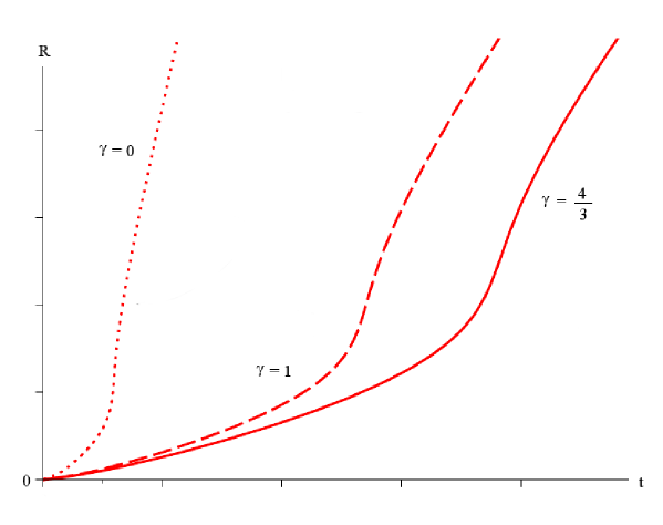
This equation is the same cubic already seen in the Schwarzschild-de Sitter/Kottler case, but now it has a time-dependent coefficient . Its roots are given again by the expression already seen, but now with time-dependent coefficient . This means that the location of the apparent horizons depends on time (i.e., on the comoving time of the FLRW “background”). Both apparent horizons exist if , an inequality which is satisfied only if . The critical time at which for a dust “background” is
| (3.56) |
There are three distinct epochs in the history of this inhomogeneous universe (Fig. 1):
-
1.
For , it is and both and are complex. There are no apparent horizons.
-
2.
The critical time corresponds to . The two roots coincide at a real value, and there exists a single apparent horizon at .
-
3.
For , it is , and there are two apparent horizons at real radii .
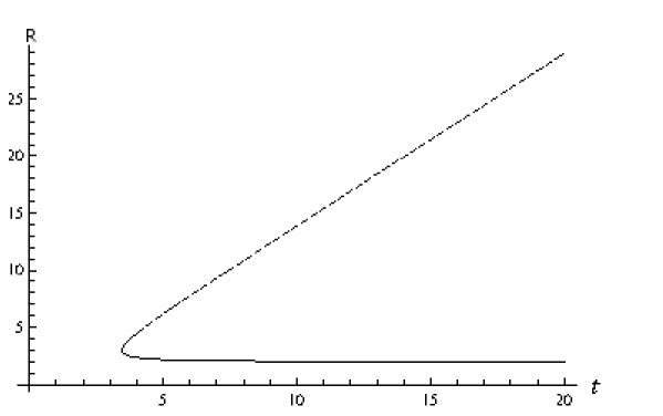
The Hubble function diverges near the Big Bang, when the mass coefficient stays supercritical at . A black hole apparent horizon cannot be accommodated in this small universe and, at there is a naked singularity at . At an instantaneous black hole apparent horizon and a cosmological apparent horizon appear together at areal radius , in analogy with the extremal Nariai black hole. As , this single horizon splits into an evolving black hole apparent horizon surrounded by an evolving cosmological horizon. The black hole apparent horizon shrinks, asymptoting to the singularity as .
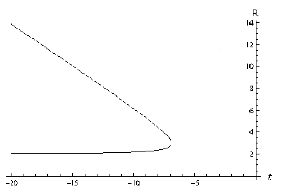
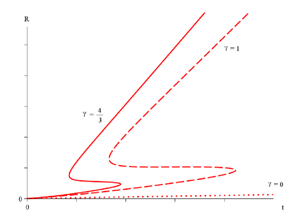
Motivated by the discovery of dark energy, and by recurrent claims by astronomers that this dark energy may have a phantom equation of state with (although such a form of dark energy seems to be in extreme conflict with known theory), one can consider a phantom “background” universe in the McVittie solution. In this case the FLRW cosmic scale factor is
| (3.57) |
where is the time of the Big Rip and is a positive constant. In this situation, the behaviour of the apparent horizons (Fig. 2) appears to be the time reversal of the behaviour already seen in a non-phantom universe.
An idealized interior solution for the McVittie exterior metric has been found [101]. It describes a relativistic star of uniform density in a FLRW “background” [101]. The equivalent of the Tolman-Oppenheimer-Volkov equation in the interior of a McVittie star is derived in [47].
Recent works on the McVittie spacetime have studied its conformal structure [76, 80, 81, 37], which entails integrating numerically the null geodesics or deriving general analytical results upon making some assumptions about the cosmic expansion. Lake & Abdelqader [80] have found that null geodesics asymptote to the singularity without entering it. Depending on the form of the scale factor, a bifurcation surface may appear which splits the spacetime boundary into a black hole horizon in the future and a white hole horizon in the past (it is not clear whether this is due directly to the McVittie no-accretion condition). da Silva, Fontanini, and Guariento [37] find that the presence of this white hole horizon depends crucially on the expansion history of the universe.
It was found recently that the McVittie geometry is also a solution of cuscuton theory, a special Hor̆ava-Lifschitz theory, and of shape dynamics [4, 58, 61].
3.2.1 Generalized McVittie solutions
It is interesting to remove the no-accretion restriction from the McVittie solutions [47]. In principle, this becomes the “Synge approach” in which one postulates a metric and runs the Einstein equations from the left to the right to derive the form of an effective stress-energy tensor that generates this metric. Usually this approach is fruitless because the effective thus generated is physically pathological and violates all the energy conditions. However, reasonable matter sources exist in this case. Assume the line element to be
| (3.58) |
where
| (3.59) | |||||
| (3.60) | |||||
| (3.61) |
and where now the new function is not determined by the McVittie no-accretion condition. The mixed Einstein tensor is
| (3.62) | |||||
| (3.63) | |||||
| (3.65) | |||||
For the special subclass of solutions which has const., the quantity
| (3.66) |
reduces to the familiar , where
| (3.67) |
this is the non-rotating Thakurta solution [128], which will re-appear later in our discussion.
At , the quantity reduces to
| (3.68) |
The McVittie solutions correspond to everywhere, while the non-rotating Thakurta solution corresponds to everywhere. The Ricci scalar
| (3.69) |
diverges at , unless is a constant.
We must now discuss the matter source. If this is a single perfect fluid, only the McVittie solutions are possible. However, imperfect fluids can be matter sources for generalized McVittie spacetimes. Two cases have been studied [47] and are reported below. In addition, since the McVittie condition has been removed and we now have a radial energy flow, we must model it somehow and an imperfect fluid is the simplest model for this purpose.
3.2.2 Imperfect fluid and no radial mass flow
In this case the right hand side of the Einstein equations (3.43) contains the matter stress-energy tensor
| (3.70) |
where the purely spatial vector describes a radial energy flow,
| (3.71) |
and . The Einstein equations yield
| (3.72) |
The radial energy flow, the area of a 2-sphere, and the accretion rate are related by [47]
| (3.73) |
In the case of inflow (), on a sphere of radius this accretion rate becomes . The mass changes due to inflow of matter and to the evolution of the cosmological fluid in it. The energy density and the pressure of the fluid are
| (3.74) | |||||
| (3.75) | |||||
The evolution of the quantity is regulated by the generalized Raychaudhuri equation [47]
| (3.76) |
3.2.3 Imperfect fluid and radial mass flow
A more general situation is the one in which both an imperfect fluid and a radial flow of material and energy are allowed, as described by the stress-energy tensor (3.70) with
| (3.77) |
(i.e., with non-vanishing radial velocity) and with spacelike flux density
| (3.78) |
In this case the accretion rate onto the central object is
| (3.79) |
and the energy density is found to be [47]
| (3.80) |
The generalized McVittie geometry is also a solution of Horndeski theory [5].
3.2.4 The non-rotating Thakurta solution
The choice selects a special subclass of generalized McVittie solutions of the Einstein equations, the non-rotating Thakurta solution [128]. The “comoving mass” attractor family coincides with the non-rotating Thakurta solution [128] of GR discovered in 1981. This is the special case, corresponding to zero angular momentum, of the Thakurta solution describing a Kerr black hole embedded in a FLRW background [128]. Recently, the non-rotating Thakurta solution has been discussed, with different purposes, in Refs. [36, 94]. The apparent horizons exhibit the same phenomenology of apparent horizons described by a C-shaped curve in the plane which appears in the McVittie spacetime and in other solutions of GR, including generalized McVittie solutions and some Lemaître-Tolman-Bondi models (keep in mind, however, that generalized McVittie geometries are also solutions of Horndeski gravity).
The non-rotating Thakurta subclass is not a mere curiosity, but it is important because it is a late-time attractor of generalized McVittie solutions [57]. Given that the Jebsen-Birkhoff theorem [75, 18] fails in the presence of matter and/or when the asymptotics are not Minkowskian, and then no “general solutions” are known, this result is significant because it provides a general solution in the generalized McVittie class, provided that one waits long enough (either in a universe expanding forever or in a phantom-dominated universe approaching a Big Rip singularity at a finite future). The non-rotating Thakurta solution is generic under certain assumptions, in the sense that all other generalized McVittie solutions approach it at late times.
Another peculiarity of this “comoving mass” Thakurta attractor resides in the structure of its apparent horizons. In general, in spherical symmetry, the radii of the apparent horizons can only be found numerically because Eq. (2.22) locating them is trascendental. It is very rare to be able to obtain analytical explicit expressions for apparent horizon radii, which would be useful, for example, for quantum field theory calculations in these curved spacetimes to determine Hawking radiation fluxes and so on. This task is possible for the non-rotating Thakurta family of solutions, for which the areal radii of the cosmological and black hole apparent horizons are [57]
| (3.81) |
3.3 The Husain-Martinez-Nuñez solution
The 1994 Husain-Martinez-Nuñez solution of the Einstein equations brings in new phenomenology of the apparent horizons with respect to what we have seen thus far. The Husain-Martinez-Nuñez spacetime describes an inhomogeneous universe with a spatially flat FLRW “background” sourced by a free, minimally coupled, scalar field. The Einstein equations (3.43) assume the form
| (3.82) |
while the free scalar field obeys the curved space Klein-Gordon equation
| (3.83) |
The Husain-Martinez-Nuñez line element is
| (3.84) | |||||
| (3.85) |
where are constants, , and . The additive constant becomes irrelevant and can be dropped if . When , the Husain-Martinez-Nuñez line element degenerates into the static Fisher one [55]
| (3.86) |
where , and are parameters, and the Fisher scalar field is
| (3.87) |
The Fisher solution also goes by the names Buchdahl-Janis-Newman-Winicour-Wyman solution because it was rediscovered many times by these authors [17, 74, 22, 136]. It always hosts a naked singularity at and is asymptotically flat. The general Husain-Martinez-Nuñez metric is conformal to the Fisher metric with conformal factor equal to the scale factor of the “background” FLRW space and with only two possible values of the parameter . In the following we set .
The Husain-Martinez-Nuñez geometry is asymptotically FLRW as and is exactly FLRW if , in which case the constant can be eliminated by rescaling the time . The Ricci scalar is
| (3.88) |
This Ricci scalar shows that there is a spacetime singularity at (for both values of the parameter ). The matter scalar field also diverges there, and there is a Big Bang singularity at .
We have and the value corresponds to zero areal radius
| (3.89) |
We can transform the time coordinate and use the comoving time of the “background” FLRW space instead of the conformal time related to by [45]. Then we have
| (3.90) | |||||
| (3.91) |
and
| (3.92) |
The Husain-Martinez-Nuñez solution in comoving time reads
| (3.93) |
| (3.94) |
The areal radius increases with for . In terms of the areal radius , and using the notation
| (3.95) |
we have
| (3.96) |
A time-radius cross-term in the line element is eliminated by introducing a new time coordinate with differential
| (3.97) |
The choice
| (3.98) |
produces
| (3.99) | |||||
The apparent horizons are located by the roots of the equation , which reads
| (3.100) |
As , corresponding to , Eq. (3.100) reduces to , the radius of the cosmological apparent horizon in FLRW.
Let , then the equation locating the apparent horizons is
| (3.101) |
The left hand side of this equation is
| (3.102) |
while the right hand side is
| (3.103) |
therefore the apparent horizons radii are expressed in parametric form by
| (3.104) | |||||
| (3.105) |
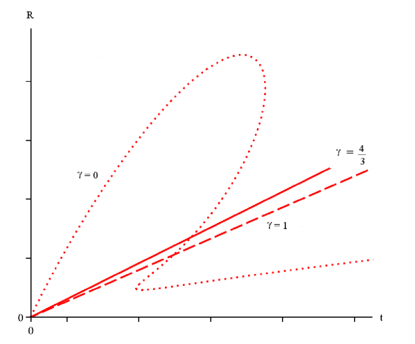
with parameter . The numerical solution for the radii of these apparent horizons is shown in Fig. 3.
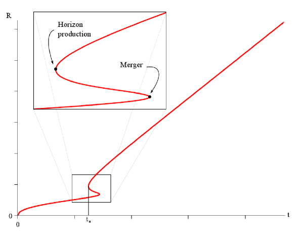
If , between the Big Bang and a critical time there is only one expanding apparent horizon, then two other apparent horizons are created at the critical comoving time . One of them is a cosmological apparent horizon which expands forever, while the other is a black hole apparent horizon which contracts until it meets the first (expanding) black hole apparent horizon [72]. When they meet, these two apparent horizons “annihilate” and a naked singularity appears at in a FLRW universe [72, 45]. This phenomenology of apparent horizons is dubbed “S-curve” behaviour from the shape of the curve representing the evolution of the apparent horizon radii in Fig. 3. This “S-curve” phenomenology appears also in Lemaître-Tolman-Bondi spacetimes, in which a dust fluid curves the cosmological “background” [21]. Multiple “S”s are also possible (e.g., five of them may appear in these Lemaître-Tolman-Bondi solutions). The scalar field is regular on the apparent horizons.
For the parameter value , there is only one cosmological apparent horizon and the universe contains a naked singularity at .
The apparent horizons are spacelike: the normal vector to these surfaces always lies inside the light cone in an diagram [72], in agreement with a general result of Booth, Brits, and Gonzalez [21] stating that a trapping horizon created by a massless scalar field must be spacelike.
The singularity at is timelike for both values of the parameter . The central black hole in this spacetime is created with the universe in the Big Bang and not in a collapse process (although sometimes the literature states otherwise).
Clifton’s 2006 solution of gravity [30] (where is the Ricci scalar) and some perfect fluid solutions of Brans-Dicke gravity found by Clifton, Mota, and Barrow [31] exhibit the same S-curve phenomenology of apparent horizons originally discovered in the Husain-Martinez-Nuñez spacetime [44, 53]. gravity is described by the fourth order field equations
| (3.106) |
where . It can be shown that theories are equivalent to a subclass of Brans-Dicke theories with effective Brans-Dicke field , coupling parameter , and the special (implicit) potential
| (3.107) |
3.4 The Fonarev and phantom Fonarev solutions
Another inhomogeneous universe representing a central object embedded in a FLRW “background” is the Fonarev solution of GR [56], which generalizes the Husain-Martinez-Nuñez spacetime (the latter has a free scalar field as the matter source) to the case in which the scalar field acquires the exponential potential
| (3.108) |
where and are positive constants. The coupled Einstein-Klein-Gordon equations are now
| (3.109) |
| (3.110) |
The Fonarev line element and scalar field are [56]
| (3.111) | |||||
| (3.112) |
where
| (3.113) | |||||
| (3.114) | |||||
| (3.115) |
and where and are constants, while is the conformal time of the FLRW substrate. Choosing and restricting to the parameter value , the Fonarev solution reduces to spatially flat FLRW. If and , it reduces to the Schwarzschild geometry, while if and , it reproduces the Husain-Martinez-Nuñez spacetime.
A generalized Fonarev solution corresponding to a phantom scalar field solution of the Einstein equations was presented in [57] and is obtained from the Fonarev solution by means of the transformation
| (3.116) |
The equation locating the apparent horizons is a quartic which has only two real positive roots, corresponding to a cosmological apparent horizon of radius and to a black hole apparent horizon of radius with the same qualitative behaviour of the apparent horizons of the (generalized) McVittie solution.
One can regard the Fonarev solution of GR as the Einstein frame version of a solution of Brans-Dicke gravity, which can then be mapped back to the Jordan frame666This is the technique used also by Clifton, Mota, and Barrow [31] to generate a conformal cousin of the Husain-Martinez-Nuñez spacetime which is a vacuum solution of Brans-Dicke theory studied in [49]. [46]. The conformal cousin of the Fonarev geometry is a 4-parameter family of solutions which are spherical, non-static, and asymptotically FLRW. The solutions of this family which have been studied explicitly contain only wormholes and naked singularities. Special cases of this 4-parameter family provide solutions of vacuum gravity [46].
3.5 Other GR solutions
Other better-known solutions of GR which may be interpreted as black holes embedded in cosmological substrata include Swiss-cheese models [40, 41], Lemaître-Tolman-Bondi black holes (with a dust-dominated FLRW “background”), members of the large Barnes family of solutions [13], and the Sultana-Dyer solution [124]. Several other analytical solutions of GR exist which describe central inhomogeneities in FLRW “backgrounds” [56, 132, 109, 114, 23, 11, 35, 83, 84]. Many do not have reasonable matter sources and the energy density becomes negative in certain spacetime regions. Often these solutions are obtained by conformally transforming a stationary black hole solution or by performing a Kerr-Schild transformation of a stationary black hole metric ,
| (3.117) |
where is a function of the spacetime position and the vector is null and geodesic with respect to both and [78, 79, 89, 90, 91, 92].
3.6 Perfect fluid solutions of Brans-Dicke gravity
Perfect fluid solutions of Brans-Dicke gravity describing dynamical cosmological black holes in certain regions of the parameter space were found by Clifton, Mota, and Barrow [31]. The Brans-Dicke field equations are
| (3.118) |
| (3.119) |
where is the Brans-Dicke coupling parameter and is the trace of the matter stress-energy tensor
| (3.120) |
describing a perfect fluid with constant equation of state
| (3.121) |
while the Brans-Dicke field is free and massless. The line element of this family of solutions is spherical, inhomogeneous, and asymptotically FLRW:
| (3.122) |
where
| (3.123) | |||||
| (3.124) | |||||
| (3.125) | |||||
| (3.126) |
while the Brans-Dicke scalar field and the fluid energy density are
| (3.127) | |||||
| (3.128) |
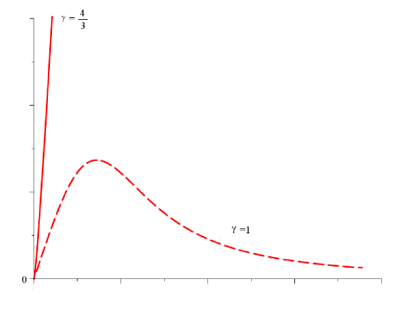
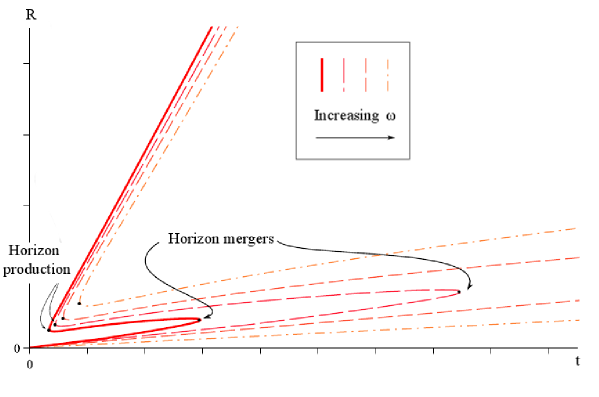
The areal radii of the apparent horizons of this class of solutions were studied in [53], disclosing a rich variety of behaviours as the three parameters vary. Some possibilities, corresponding to selected regions of parameter space, are shown in Figs. 4-7 (we refer the reader to [53] for details).
3.7 Is there a relation between S-curve and C-curve?
Thus far, we have encountered two main phenomenological classes describing the time behaviour of apparent horizons in spherical inhomogeneus spacetimes: the “C-curve” behaviour exemplified by McVittie solutions and the “S-curve” phenomenology originally discovered in the Husain-Martinez-Nuñez solution of GR. These two phenomenologies are encountered in GR and in other theories of gravity. We know that other behaviours are in principle possible (cf. Sec. 3.6) and that the catalog of analytic solutions with these physical properties is scarce in GR and even leaner in alternative theories of gravity. However, the tentative assumption that these two behaviours have some generality has some basis for the moment. One is then led to wonder whether the “S-curve” and the “C-curve” behaviours are completely disconnected and mutually exclusive, or whether there may be some relation between them. As the Brans-Dicke coupling tends to infinity, the Clifton-Mota-Barrow solution of Brans-Dicke gravity discussed in the previous subsection asymptotes to the comoving mass non-rotating Thakurta solution of GR [45]. While the limit of Brans-Dicke theory is expected to reproduce a corresponding GR solution [135], exceptions are known [88, 116, 117, 118, 107, 6] and often explained [12, 42, 43]. In this case the non-rotating Thakurta solution is indeed the GR limit of the Clifton-Mota-Barrow solution, which was not realized nor expected a priori. But the most interesting thing is the behaviour of the apparent horizons of the Clifton-Mota-Barrow geometry in this limit: the S-curve describing the apparent horizons areal radii in the plane reduces to a C-curve as because the lower bend of the S-curve is pushed to infinity [48], as shown in Fig. 8.
Is the C-curve described by the apparent horizons radii of a spherical, asymptotically FLRW spacetime always a limit of an S-curve? Does the relation between these two phenomenologies have any physical meaning or are we just looking at a coincidence? These questions are currently under investigation.
4 Conclusions
To conclude this brief excursion on the subject of dynamical cosmological black holes and their relations with modified gravity, one should first realize that, while it is auspicable to find new inhomogeneous solutions amenable to this physical interpretation, it is usually harder to find whether apparent horizons exist, and to determine their location, nature, and dynamical behaviour, and some effort should be devoted to these goals.
There are many open questions, some of which are more general than the subject of dynamical cosmological black holes, and are related to the nature of horizons, which ultimately define the very concept of black hole. The main question seem to be whether apparent horizons are the “right” surfaces to characterize black holes. It is a fact that apparent and trapping horizons are used in the numerical prediction of the waveforms of gravitational waves emitted by binary systems and used in their interferometric detection. The recent successes of the LIGO interferometers [1, 2, 3] in detecting the elusive gravitational waves from black hole mergers seem to answer the question affirmatively, but it is in principle possible that a different notion of horizon could be as successful as that of apparent/trapping horizon. In the meantime, the gravitational wave community is not apologetic in using apparent and trapping horizons and in disregarding the teleological event horizon.
A different but related question, which has not been addressed here, is whether apparent horizons are the “right” surfaces to use in the study of the thermodynamics of dynamical black holes. There are strong claims that they are, but no convincing definitive proof has been provided. It is difficult to perform calculations of quantum field theory in curved space even on a prescribed time-dependent black hole background (that is, neglecting backreaction). The situation at the moment is summarized in the fact that the tunneling method provides a definite and general result for the Hawking temperature while other methods, at best, have produced results only for specific and very particular background metrics and a general computation cannot be completed as is done in the tunneling method. However, at present there is no guarantee that the result and procedure provided by the tunneling method are actually correct. Progress in this direction is very slow. At the very least, apparent horizons would require some adiabatic approximation if they are to make sense for dynamical black holes, otherwise one is probably discussing non-equilibrium thermodynamics, which is a tall order in the context of a problem which is proving to be already very difficult in equilibrium thermodynamics.
Assuming that apparent horizons are the “correct” notion of horizon, their biggest problem is no doubt their foliation-dependence, which amounts to the fact that the very existence of a black hole seems to depend on the observer. This problem is exemplified dramatically by the realization that there exist slicings of the Schwarzschild spacetime with no apparent horizons [134, 120]. The fact that these slicings are rather contrived is not of much consolation. From the practical point of view, the problem is mitigated by the fact that, in spherical symmetry, the apparent horizons coincide in all spherically symmetric foliations [51], but this fact does not really solve the problem and, moreover, no analogous result has been proved beyond spherical symmetry.
In our examples of apparent horizon phenomenology, we have restricted ourselves to spherical symmetry. Evolving apparent horizons exhibit a rather rich phenomenology and dynamics, but there seem to be two main phenomenological classes for the behaviour of the areal radii of apparent horizons versus the comoving time of the FLRW substratum in which the spherical inhomogeneities are embedded. These are the “C-curve” first encountered in the McVittie spacetime of GR [93] and the “S-curve” first discovered in the Husain-Martinez-Nuñez solution of the same theory [72] and then rediscovered in and Brans-Dicke gravity [44, 53]. There are hints that some relation may exist between these two classes, with the C-curve being some limit of the S-curve, but the situation is not clear at present.
A final question is provided by the long-standing issue of cosmic expansion versus local dynamics which motivated the introduction of the McVittie metric in 1933 and of the Einstein-Straus Swiss-cheese model a decade later. This problem of principle, which at some point was brushed off as being irrelevant, keeps being discussed in the literature (see [25] for a 2010 review). We have seen already in the few examples discussed here that sometimes black hole apparent horizons expand (in rare cases they are even comoving with the cosmic substratum), whereas some other times they resist the cosmic expansion or even contract. No general rule appears here and the apparent horizons of dynamical cosmological black holes provide no definite answer to the puzzle. All these theoretical questions of classical gravity are worth understanding and investigating in the future. The recent detection of gravitational waves and the future development of gravitational wave astronomy seem to reformulate the issue of apparent horizons in more practical terms and to make its understanding a more pressing issue than it was before.
Acknowledgments
The author thanks Angus Prain for producing an earlier version of most figures, a referee for helpful comments, and Bishop’s University for support.
References
- [1] Abbott, B.P. et al. (LIGO Scientific Collaboration and Virgo Collaboration). Observation of Gravitational Waves from a Binary Black Hole Merger. Phys. Rev. Lett. 2016, 116, 061102, doi:10.1103/PhysRevLett.116.061102.
- [2] Abbott, B.P.et al. (LIGO Scientific Collaboration and Virgo Collaboration). GW151226: Observation of Gravitational Waves from a 22-Solar-Mass Binary Black Hole Coalescence. Phys. Rev. Lett. 2016, 116, 241103, doi:10.1103/PhysRevLett.116.241103.
- [3] Abbott, B.P. et al. (LIGO Scientific and Virgo Collaboration). GW170104: Observation of a 50-Solar-Mass Binary Black Hole Coalescence at Redshift 0.2. Phys. Rev. Lett. 2017, 118, 221101, doi:10.1103/PhysRevLett.118.221101.
- [4] Abdalla, E., Afshordi, N., Fontanini, M., Guariento, D.C., Papantonopoulos, E. Cosmological black holes from self-gravitating fields. Phys. Rev. D 2014, 89, 104018, doi:10.1103/PhysRevD.89.104018.
- [5] Afshordi, N., Fontanini, M., Guariento, D.C. Horndeski meets McVittie: a scalar field theory for accretion onto cosmological black holes. Phys. Rev. D 2014, 90, 084012, doi:10.1103/PhysRevD.90.084012.
- [6] Anchordoqui, L.A., Torres, D.F., Trobo, M.L., Perez-Bergliaffa, S.E. Evolving wormhole geometries. Phys. Rev. D 1998, 57, 829-833, doi:10.1103/PhysRevD.57.829.
- [7] Ashtekar, A., Krishnan, B. Isolated and dynamical horizons and their applications. Living Rev. Relat. 2004, 7, 10, doi:10.12942/lrr-2004-10.
- [8] Babichev, E., Chernov, Dokuchaev, V., Eroshenko, Yu. Perfect fluid and scalar field in the Reissner-Nordstrom metric. J. Exp. Theor. Phys. 2011, 112, 784, doi:10.1134/S1063776111040157.
- [9] Babichev, E., Dokuchaev, V., Eroshenko, Yu. Black hole mass decreasing due to phantom energy accretion. Phys. Rev. Lett. 2004, 93, 021102, oi:10.1103/PhysRevLett.93.021102.
- [10] Balbinot, R., Hawking radiation and the back reaction—a first approach. Class. Quantum Grav. 1984, 1, 573-577, doi:10.1088/0264-9381/1/5/010.
- [11] Balbinot, R., Bergamini, R., Comastri, A. Solution of the Einstein-Strauss problem with a term. Phys. Rev. D 1988, 38, 2415-2418, doi:10.1103/PhysRevD.38.2415.
- [12] Banerjee, N. and Sen, S. Does Brans-Dicke theory always yield general relativity in the infinite limit? Phys. Rev. D 1997, 56, 1334, doi:10.1103/PhysRevD.56.1334.
- [13] Barnes, A. On shear free normal flows of a perfect fluid. Gen. Relat. Gravit. 1973, 2, 105-129.
- [14] Baumgarte, T.W., Shapiro, S.L. Numerical relativity and compact binaries. Phys. Rept. 2003, 376, 41-131, doi:10.1016/S0370-1573(02)00537-9.
- [15] Ben-Dov, I. Outer trapped surfaces in Vaidya spacetimes. Phys. Rev. D 2007, 75, 064007, doi:10.1103/PhysRevD.70.124031.
- [16] Bengtsson, I., Senovilla, J.M.M., Region with trapped surfaces in spherical symmetry, its core, and their boundaries. Phys. Rev. D 2011, 83, 044012, doi:10.1103/PhysRevD.83.044012.
- [17] Bergman O., Leipnik, R. Space-Time Structure of a Static Spherically Symmetric Scalar Field Phys. Rev. 1957, 107, 1157-1161, doi:10.1103/PhysRev.107.1157.
- [18] Birkhoff, G.D., Relativity and Modern Physics. Cambridge, USA: Harvard University Press, 1923, p. 253.
- [19] Bolejko, K., Celerier, M.-N., Krasínski, A. Inhomogeneous cosmological models: exact solutions and their applications. Class. Quantum Grav. 2011, 28, 164002, doi:10.1088/0264-9381/28/16/164002.
- [20] Booth, I. Black hole boundaries. Can. J. Phys. 2005, 83, 1073, doi:10.1139/p05-063.
- [21] Booth, I., Brits, L., Gonzalez, J.A., Van den Broeck, V. Marginally trapped tubes and dynamical horizons. Class. Quantum Grav. 2006, 23, 413, doi:10.1088/0264-9381/28/16/164002.
- [22] Buchdahl, H.A. Static solutions of the Brans-Dicke equations. Int. J. Theor. Phys. 1972, 6, 407-412, doi:10.1007/BF01258735.
- [23] Burko, L.M., Ori A. (eds.). Internal Structure of Black Holes and Spacetime Singularities, An International Research Workshop, Haifa 1997. Bristol: IOP, 1997.
- [24] Capozziello, S., Carloni, S., Troisi, A. Quintessence without scalar fields. Recent Res. Dev. Astron. Astrophys. 2003, 1, 625.
- [25] Carrera, M., Giulini, D. Influence of global cosmological expansion on local dynamics and kinematics. Rev. Mod. Phys. 2010, 82, 169-208, doi:10.1103/RevModPhys.82.169.
- [26] Carroll, S.M., Duvvuri, V., Trodden, M., Turner, M.S. Is cosmic speed-up due to new gravitational physics? Phys. Rev. D 2004, 70, 043528, doi:10.1103/PhysRevD.70.043528.
- [27] Chadburn, S., Gregory, R. Time dependent black holes and scalar hair. Class. Quantum Grav. 2014, 31, doi:10.1088/0264-9381/31/19/195006.
- [28] Chen, S., Jing, J. Quasinormal modes of a black hole surrounded by quintessence. Class. Quantum Grav. 2005, 22, 4651-4657, doi:10.1088/0264-9381/22/21/011.
- [29] Chu, T., Pfeiffer, H.P., Cohen, M.I. Horizon dynamics of distorted rotating black holes. Phys. Rev. D 2011, 83, 104018, doi:10.1103/PhysRevD.83.104018.
- [30] Clifton, T. Spherically symmetric solutions to fourth-order theories of gravity. Class. Quantum Grav. 2006, 23, 7445-7453, doi:10.1088/0264-9381/23/24/015.
- [31] Clifton, T., Mota, D.F., Barrow, J.D. Inhomogeneous gravity. Mon. Not. R. Astr. Soc. 2005, 358, 601-613, doi:10.1111/j.1365-2966.2005.08831.x.
- [32] Collins, W. Mechanics of apparent horizons. Phys. Rev. D 1992, 45, 495-498, doi:10.1103/PhysRevD.45.495.
- [33] W.G. Cook, D. Wang, U. Sperhake Orbiting black-holes and apparent horizons in higher dimensions. arXiv:1808.05834.
- [34] Corichi, A., Sudarsky, D. When is ?, Mod. Phys. Lett. A 2002, 17, 1431-1444, doi:10.1142/S0217732302007843.
- [35] Cox, D.P.G. Vaidya’s Kerr-Einstein metric cannot be matched to the Kerr metric. Phys. Rev. D 2003, 68, 124008, doi:10.1103/PhysRevD.68.124008.
- [36] Culetu, H. On the conformal version of Schwarzschild-de Sitter spacetime. J. Phys. Conf. Ser. 2013, 437, 012005.
- [37] da Silva, A., Fontanini, M., Guariento, D.C. How the expansion of the universe determines the causal structure of McVittie spacetimes. Phys. Rev. D 2013, 87, 064030, doi:10.1103/PhysRevD.87.064030.
- [38] De Felice, A., Tsujikawa, S. theories. Living Rev. Relativ. 2010, 13, 3-161, doi:10.12942/lrr-2010-3.
- [39] de Freitas Pacheco, J.A., Horvath, J.E. Generalized second law and phantom cosmology. Class. Quantum Grav. 2007, 24, 5427-5434, doi:10.1088/0264-9381/24/22/007.
- [40] Einstein, A., Straus, E.G. The influence of the expansion of space on the gravitation fields surrounding the individual stars. Rev. Mod. Phys. 1945, 17, 120-124, doi:10.1103/RevModPhys.17.120.
- [41] Einstein, A., Straus, E.G. Corrections and additional remarks to our paper: the influence of the expansion of space on the gravitation fields surrounding the individual stars. Rev. Mod. Phys. 1946, 18, 148-149, doi:10.1103/RevModPhys.18.148.
- [42] Faraoni, V. The limit of Brans-Dicke theory. Phys. Lett. A 1998, 245, 26-30, doi:10.1016/S0375-9601(98)00387-9.
- [43] Faraoni, V. Illusions of general relativity in Brans-Dicke gravity. Phys. Rev. D 1999, 59, 084021, doi:10.1103/PhysRevD.59.084021.
- [44] Faraoni, V. Clifton’s spherical solution in vacuum harbours a naked singularity. Class. Quantum Grav. 2009, 26, 195013, doi:10.1088/0264-9381/26/19/195013.
- [45] Faraoni, V., Cosmological and Black hole Apparent Horizons. New York: Springer, 2015, doi:10.1007/978-3-319-19240-6.
- [46] Faraoni, V., Belknap-Keet, S.D. New inhomogeneous universes in scalar-tensor and gravity. Phys. Rev. D 2017, 96, 044040, doi:10.1103/PhysRevD.96.044040.
- [47] Faraoni, V., Jacques, A. Cosmological expansion and local physics. Phys. Rev. D 2007, 76, 063510, doi:10.1103/PhysRevD.76.063510.
- [48] Faraoni, V., Prain, A. Understanding dynamical black hole apparent horizons. arXiv:1511.07775.
- [49] Faraoni, V., Zambrano Moreno, A.F. Interpreting the conformal cousin of the Husain-Martinez-Nuñez solution. Phys. Rev. D 2012, 86, 084044, doi:10.1103/PhysRevD.86.084044.
- [50] Faraoni, V., Cardini, A.M., Chung, W.-J. Simultaneous baldness and cosmic baldness and the Kottler spacetime. Phys. Rev. D 2018, 97, 024046, doi:10.1103/PhysRevD.97.024046.
- [51] Faraoni, V., Ellis, G.F.R., Firouzjaee, J.T., Helou, A., Musco, I. Foliation dependence of black hole apparent horizons in spherical symmetry. Phys. Rev. D 2017, 95, 024008, doi:10.1103/PhysRevD.95.024008.
- [52] Faraoni, V., Gao, C., Chen, X., Shen, Y.-G. What is the fate of a black hole embedded in an expanding universe? Phys. Lett. B 2009, 671, 7-9, doi:10.1016/j.physletb.2008.11.067.
- [53] Faraoni, V., Vitagliano, V. Sotiriou, T.P., Liberati, S. Dynamical apparent horizons in inhomogeneous Brans-Dicke universes. Phys. Rev. D 2012, 86, 064040, doi:10.1103/PhysRevD.86.064040.
- [54] Faraoni, V., Zambrano Moreno, A.F., Nandra, R. Making sense of the bizarre behavior of horizons in the McVittie spacetime. Phys. Rev. D 2012, 85, 083526, doi:10.1103/PhysRevD.85.083526.
- [55] Fisher, I.Z. Scalar mesostatic field with regard for gravitational effects. Zh. Eksp. Teor. Fiz. 1948, 18, 636-640, translated in arXiv:gr-qc/9911008.
- [56] Fonarev, O.A. Exact Einstein scalar field solutions for formation of black holes in a cosmological setting. Class. Quantum Grav. 1995, 12, 1739-1752, doi:10.1088/0264-9381/12/7/016.
- [57] Gao, C., Chen, X., Faraoni, V., Shen, Y.-G. Does the mass of a black hole decrease due to accretion of phantom energy? Phys. Rev. D 2008, 78, 024008, doi:10.1103/PhysRevD.78.024008.
- [58] Gomes, H., Gryb, S., Koslowski, T. Einstein gravity as a 3D conformally invariant theory. Class. Quantum Grav. 2011, 28, 045005, doi:10.1088/0264-9381/28/4/045005.
- [59] Gonzalez, J.A., Guzman, F.S. Accretion of phantom scalar field into a black hole. Phys. Rev. D 2009, 79, 121501, doi:10.1103/PhysRevD.79.121501.
- [60] Gourghoulhon, E., Jaramillo, J.L. New theoretical approaches to black holes. New Astron. Rev. 2008, 51, 791-798, doi:10.1016/j.newar.2008.03.026.
- [61] Guariento, D.C., Mercati, F. Cosmological self-gravitating fluid solutions of shape dynamics. Phys. Rev. D 2016, 94, 064023, doi:10.1103/PhysRevD.94.064023.
- [62] Guariento, D.C., Horvath, J.E., Custodio, P.S., de Freitas Pacheco, J.A. Evolution of primordial black holes in a radiation and phantom energy environment. Gen. Relat. Gravit. 2008, 40, 1593-1602, doi:10.1007/s10714-007-0562-8.
- [63] Haijcek, P. Origin of Hawking radiation. Phys. Rev. D 1987, 36, 1065-1107, doi:10.1103/PhysRevD.36.1065.
- [64] Hawking, S.W. Gravitational radiation in an expanding universe. J. Math. Phys. 1968, 9, 598-604, doi:10.1063/1.1664615.
- [65] Hayward, S.A. Quasilocal gravitational energy. Phys. Rev. D 1994, 49, 831-839, doi:10.1103/PhysRevD.49.831.
- [66] Hayward, S.A. General laws of black hole dynamics. Phys. Rev. D 1994, 49, 6467-6474, doi:10.1103/PhysRevD.49.6467.
- [67] Hayward, S.A. Formation and Evaporation of Nonsingular Black Holes. Phys. Rev. Lett. 2006, 96, 031103, doi:10.1103/PhysRevLett.96.031103.
- [68] He, X., Wang, B., Wu, S.-F., Lin, C.-Y. Quasinormal modes of black holes absorbing dark energy. Phys. Lett. B 2009, 673, 156-160, doi:10.1016/j.physletb.2009.02.002.
- [69] Herdeiro, C.A.R., Radu, E. Asymptotically flat black holes with scalar hair: A review. Int. J. Mod. Phys. D 2015, 24, 1542014, doi:10.1142/S0218271815420146.
- [70] Hernandez, W.C., Misner, C.W. Observer time as a coordinate in relativistic spherical hydrodynamics. Astrophys. J. 1966, 143, 452-464, doi:10.1086/148525.
- [71] Hiscock, W.A. Gravitational entropy of nonstationary black holes and spherical shells. Phys. Rev. D 1989, 40, 1336-1339, doi:10.1103/PhysRevD.40.1336.
- [72] Husain, V., Martinez, E.A., Nuñez, D. Exact solution for scalar field collapse. Phys. Rev. D 1994, 50, 3783-3786, doi:10.1103/PhysRevD.50.3783.
- [73] Izquierdo, G., Pavon, D. The generalized second law in phantom dominated universes in the presence of black holes. Phys. Lett. B 2006, 639, 1-4, doi:10.1016/j.physletb.2006.05.082.
- [74] Janis, A.I., Newman, E.T., Winicour, J. Reality of the Schwarzschild Singularity. Phys. Rev. Lett. 1968, 20, 878-880, doi:10.1103/PhysRevLett.20.878.
- [75] Jebsen, J.T. On the General Spherically Symmetric Solutions of Einstein’s Gravitational Equations in Vacuo. Ark. Mat. Ast. Fys. (Stockholm) 1921, 15, nr. 18. Reprinted in Gen. Relat. Gravit. 2005, 37, 2253.
- [76] Kaloper, N., Kleban, M., Martin, D. McVittie’s legacy: black holes in an expanding universe. Phys. Rev. D 2010, 81, 104044, doi:10.1103/PhysRevD.81.104044.
- [77] Kottler, F. Über die physikalischen Grundlagen der Einsteinschen gravitationstheorie. Ann. Phys. (Leipzig) 1918, 361, (14) 401-462.
- [78] Krasiński, A. Inhomogeneous Cosmological Models. Cambridge: Cambridge University Press, 1997.
- [79] Krasínski, A., Hellaby, C. Formation of a galaxy with a central black hole in the Lematre-Tolman model. Phys. Rev. D 2004, 69, 043502, doi:10.1103/PhysRevD.69.043502.
- [80] Lake, K., Abdelqader, M. More on McVittie’s legacy: a Schwarzschild-de Sitter black and white hole embedded in an asymptotically CDM cosmology. Phys. Rev. D 2011, 84, 044045, doi:10.1103/PhysRevD.84.044045.
- [81] Landry, P., Abdelqader, M., Lake, K. McVittie solution with a negative cosmological constant. Phys. Rev. D 2012, 86, 084002, doi:10.1103/PhysRevD.86.084002.
- [82] Li, Z.-H., Wang, A. Existence of black holes in Friedmann-Robertson-Walker universe dominated by dark energy. Mod. Phys. Lett. A 2007, 22, 1663-1676, doi:10.1142/S0217732307024048.
- [83] Lindesay, J. Coordinates with Non-Singular Curvature for a Time Dependent Black Hole Horizon. Found. Phys. 2007, 37, 1181-1196, doi:10.1007/s10701-007-9146-4.
- [84] Lindesay, J., Foundations of Quantum Gravity (Cambridge University Press, Cambridge, 2013, p. 282.
- [85] Maeda, H. Final fate of spherically symmetric gravitational collapse of a dust cloud in Einstein-Gauss-Bonnet gravity. Phys. Rev. D 2006, 73, 104004, doi:10.1103/PhysRevD.73.104004.
- [86] Maeda, H., Nozawa, M. Generalized Misner-Sharp quasilocal mass in Einstein-Gauss-Bonnet gravity. Phys. Rev. D 2008, 77, 064031, doi:10.1088/0264-9381/25/5/055009.
- [87] Maeda, H., Harada, T., Carr, B.J. Self-similar cosmological solutions with dark energy. II. Black holes, naked singularities, and wormholes. Phys. Rev. D 2008, 77, 024023, doi:10.1103/PhysRevD.77.024023.
- [88] Matsuda, T. On the Gravitational Collapse in Brans-Dicke Theory of Gravity. Progr. Theor. Phys. 1972, 47, 738, doi:10.1143/PTP.47.738.
- [89] McClure, M.L., Dyer, C.C. Asymptotically Einstein-de Sitter cosmological black holes and the problem of energy conditions. Class. Quantum Grav. 2006, 23, 1971-1987, doi:10.1088/0264-9381/23/6/008.
- [90] McClure, M.L., Dyer, C.C. Matching radiation-dominated and matter-dominated Einstein-de Sitter universes and an application for primordial black holes in evolving cosmological backgrounds. Gen. Relat. Gravit. 2006, 38, 1347-1354, doi:10.1007/s10714-006-0321-2.
- [91] McClure, M.L., Anderson, K., Bardahl, K. Cosmological versions of Vaidya’s radiating stellar exterior, an accelerating reference frame, and Kinnersley’s photon rocket. arXiv:0709.3288.
- [92] McClure, M.L., Anderson, K., Bardahl, K. Nonisolated dynamical black holes and white holes. Phys. Rev. D 2008, 77, 104008, doi:10.1103/PhysRevD.77.104008.
- [93] McVittie, G.C. The mass-particle in an expanding universe. Mon. Not. R. Astr. Soc. 1933, 93, 325-339, doi:10.1093/mnras/93.5.325.
- [94] Mello, M.M.C., Maciel, A., Zanchin, V.T. Evolving black holes from conformal transformations of static solutions. Phys. Rev. D 2017, 95, 084031, doi:10.1103/PhysRevD.95.084031.
- [95] Misner, C.W., Sharp, D.H. Relativistic equations for adiabatic, spherically symmetric gravitational collapse. Phys. Rev. 1964, 136, B571-B576, doi:10.1103/PhysRev.136.B571.
- [96] Nielsen, A.B. Black holes and black hole thermodynamics without event horizons. Gen. Relat. Gravit. 2009, 41, 1539-1584, doi:10.1007/s10714-008-0739-9.
- [97] Nielsen, A.B., Revisiting Vaidya horizons, Galaxies 2014, 2, 62-71, doi:10.3390/galaxies2010062.
- [98] Nielsen, A.B., Firouzjaee, J.T. Conformally rescaled spacetimes and Hawking radiation. Gen. Relat. Gravit. 2013, 45, 1815-1838, doi: 10.1007/s10714-013-1560-7.
- [99] Nielsen, A.B., Yoon, J.H. Dynamical surface gravity. Class. Quantum Grav. 2008, 25, 085010, doi:10.1088/0264-9381/25/8/085010.
- [100] Nielsen, A.B., Visser, M. Production and decay of evolving horizons, Class. Quantum Grav. 2006, 23, 4637, doi:10.1088/0264-9381/23/14/006.
- [101] Nolan, B.C. Sources for McVittie’s mass particle in an expanding universe. J. Math. Phys. 1993, 34, 178-185.
- [102] Nolan, B.C. A Point mass in an isotropic universe: existence, uniqueness and basic properties. Phys. Rev. D 1998, 58, 064006, doi:10.1103/PhysRevD.58.064006.
- [103] Nolan, B.C. A Point mass in an isotropic universe. 2. Global properties. Class. Quantum Grav. 1999, 16, 1227-1254, doi:10.1088/0264-9381/16/4/012.
- [104] Nolan, B.C. A Point mass in an isotropic universe 3. The region . Class. Quantum Grav. 1999, 16, 3183-3191, doi:10.1088/0264-9381/16/10/310.
- [105] Nouicer, K. Hawking radiation and thermodynamics of dynamical black holes in phantom dominated universe. Class. Quantum Grav. 2011, 28, 015005, doi:10.1088/0264-9381/28/1/015005..
- [106] Nojiri, S., Odintsov, S.D., Unified cosmic history in modified gravity: From theory to Lorentz non-invariant models. Phys. Repts. 2011, 505, 59-144, doi:10.1016/j.physrep.2011.04.001.
- [107] Paiva, F.M. and Romero, C. The limits of Brans-Dicke spacetimes: a coordinate-free approach. Gen. Relat. Gravit. 1993, 25, 1305.
- [108] Parikh, M.K., Wilczek, F. Hawking radiation as tunneling. Phys. Rev. Lett. 2000, 85, 5042, doi:10.1103/PhysRevLett.85.5042.
- [109] Patel, L.K., Trivedi, H.B. Kerr-Newman metric in cosmological background. J. Astrophys. Astr. 1982, 3, 63-67.
- [110] Penrose, R. Gravitational collapse and spacetime singularities. Phys. Rev. Lett. 1965, 14, 57-59.
- [111] Pielhan, M., Kunstatter, G., Nielsen, A.B. Dynamical surface gravity in spherically symmetric black hole formation. Phys. Rev. D 2011, 84, 104008, doi:10.1103/PhysRevD.84.104008.
- [112] Poisson, E. A Relativist’s Toolkit: The Mathematics of Black-Hole Mechanics. Cambridge: Cambridge University Press, 2004.
- [113] Rindler, W. Visual horizons in world-models. Mon. Not. R. Astr. Soc. 1956, 116, 663-677. Reprinted in Gen. Relat. Gravit. 2002, 34, 133-153, doi:10.1023/A:1015347106729.
- [114] Roberts, M.D. Scalar field counterexamples to the Cosmic Censorship hypothesis. Gen. Relat. Gravit. 1989, 21, 907-939, doi:10.1007/BF00769864.
- [115] Roman, T.A., Bergmann, P.G. Stellar collapse without singularities?. Phys. Rev. D 1983, 28, 1265-1277, doi:10.1103/PhysRevD.28.1265.
- [116] Romero, C., Barros, A. Brans-Dicke cosmology and the cosmological constant: the spectrum of vacuum solutions. Astrophys. Sp. Sci. 1991, 192, 263, doi:10.1007/BF00684484.
- [117] Romero, C., Barros, A. Does the Brans-Dicke theory of gravity go over to general relativity when ? Phys. Lett. A 1993, 173, 243, doi:10.1016/0375-9601(93)90271-Z.
- [118] Romero, C., Barros, A. Brans-Dicke vacuum solutions and the cosmological constant: A qualitative analysis. Gen. Relat. Gravit. 1993, 25, 491, doi:10.1007/BF00756968.
- [119] Schleich, K., Witt, D. M. A simple proof of Birkhoff’s theorem for cosmological constant. J. Math. Phys. (N.Y.) 2010, 51, 112502, doi:10.1063/1.3503447.
- [120] Schnetter, E., Krishnan, B. Non-symmetric trapped surfaces in the Schwarzschild and Vaidya spacetimes. Phys. Rev. D 2006, 73, 021502, doi:10.1103/PhysRevD.73.021502.
- [121] Sorkin, R.D. How wrinkled is the surface of a black hole?, in Proceedings of the First Australasian Conference on General Relativity and Gravitation, February 1996, D. Wiltshire ed. Adelaide, Australia: (University of Adelaide, 1996, pp. 163-174 [arXiv:gr-qc/9701056].
- [122] Sotiriou, T.P. Black holes and scalar fields. Class. Quantum Grav. 2015, 32, 214002, doi:10.1088/0264-9381/32/21/214002.
- [123] Sotiriou, T.P., Faraoni, V., theories of gravity. Rev. Mod. Phys. 2010, 82, 451-497, doi:10.1103/RevModPhys.82.451.
- [124] Sultana, J., Dyer, C.C. Cosmological black holes: A black hole in the Einstein-de Sitter universe. Gen. Relat. Gravit. 2005, 37, 1349-1370, doi:10.1007/s10714-005-0119-7.
- [125] Sun, C.-Y. Phantom energy accretion onto black holes in a cyclic universe. Phys. Rev. D 2008, 78, 064060, doi:10.1103/PhysRevD.78.064060.
- [126] Sun, C.-Y. Dark Energy accretion onto a black hole in an expanding universe. Comm. Theor. Phys. 2009, 52, 441-444, doi:10.1088/0253-6102/52/3/12.
- [127] Synge, J. L. Relativity: The General Theory. Amsterdam: North Holland, 1960.
- [128] Thakurta, S.N.G. Kerr metric in an expanding universe. Indian J. Phys. 1981, 55B, 304.
- [129] Thornburg, J. Event and apparent horizon finders for 3+1 numerical relativity. Living Rev. Relat. 2007, 10, 3.
- [130] Tretyakova, D.A., Latosh, B.N. Scalar-tensor black holes in an expanding universe. Universe 2018. 4, 26, doi:10.3390/universe4020026.
- [131] Vaidya, P. The gravitational field of a radiating star. Proc. Indian Acad. Sci. Sect. A 1951, 33, 264276.
- [132] Vaidya, P.C. The Kerr metric in cosmological background. Pramana 1977, 8, 512-517.
- [133] Wald, R.M. General Relativity. Chicago; Chicago University Press, 1984.
- [134] Wald, R.M., Iyer, V. Trapped surfaces in the Schwarzschild geometry and cosmic censorship. Phys. Rev. D 1991, 44, R3719-R3722, doi:10.1103/PhysRevD.44.R3719.
- [135] Weinberg, S. Gravitation and Cosmology. New York: Wiley, 1972.
- [136] Wyman, M. Static spherically symmetric scalar fields in general relativity. Phys. Rev. D 1981, 24, 839-841, doi:10.1103/PhysRevD.24.839.
- [137] Zhou, S., Liu, W. Apparent horizon and event horizon of a Vaidya black hole. Mod. Phys. Lett. A 2009, 24, 2099-2106, doi:10.1142/S0217732309030709.