Non-linear process convolutions for multi-output Gaussian processes

Mauricio A Álvarez1   Wil O C Ward1   Cristian Guarnizo2
1Department of Computer Science, University of Sheffield, UK
2Faculty of Engineering, Universidad Tecnológica de Pereira, Colombia
Corresponding author: mauricio.alvarez@sheffield.ac.uk.
MAA and WW have been financed by the Engineering and Physical Research Council (EPSRC) Research Project EP/N014162/1. MAA has also been financed by the EPSRC Research Project EP/R034303/1. CG would like to thank Convocatoria 567 from Administrative Department of Science, Technology and Innovation of Colombia (COLCIENCIAS) for the financial support.
Abstract

The paper introduces a non-linear version of the process convolution formalism for building covariance functions for multi-output Gaussian processes. The non-linearity is introduced via Volterra series, one series per each output. We provide closed-form expressions for the mean function and the covariance function of the approximated Gaussian process at the output of the Volterra series. The mean function and covariance function for the joint Gaussian process are derived using formulae for the product moments of Gaussian variables. We compare the performance of the non-linear model against the classical process convolution approach in one synthetic dataset and two real datasets.

1 INTRODUCTION

A multi-output Gaussian process (MOGP) is a Gaussian process (GP) with a covariance function that accounts for dependencies between multiple and related outputs (Bonilla et al., 2008). Having models that exploit such dependencies is particularly important when some of the outputs are expensive to measure and the other more inexpensive outputs can be used as surrogates of the expensive output to improve its prediction. A typical example comes from geostatistics, where the accuracy of predicting the concentration of toxic heavy metals like lead or copper, which can be expensive to measure, can be improved by including measurements of pH as secondary variables, something that is significantly less expensive to measure (Goovaerts, 1997).

One of the challenges in multi-output GPs is defining a cross-covariance function between outputs that leads to a valid covariance function for the joint GP. There is extensive literature looking at ways to build such types of cross-covariance functions (Álvarez et al., 2012). One such approach is known as process convolution, for which each output is the convolution integral between a smoothing kernel and a latent random process. The approach was introduced by Barry and Ver Hoef (1996) to build covariance functions for single-output GPs, and later for multi-outputs in Ver Hoef and Barry (1998) and Higdon (2002). The convolution integral linearly transforms the underlying latent process, which is usually assumed to be a Gaussian process. The output process is then a GP with a covariance equal to the convolution operators acting to modify the covariance function of the latent GP.

The main contribution in this paper is the introduction of a non-linear version of the process convolution construction suitable both for single-output and multi-output GPs. The non-linear model is constructed using a Volterra series where the input function is a latent random process. The Volterra series has been widely studied in the literature of non-linear dynamical systems (Haber and Keviczky, 1999). They generalise the Taylor expansion for the case of non-instantaneous input functions. We treat the latent process as a Gaussian process and, using formulae for the product moments of Gaussian variables, we provide closed-form expressions for the mean function and covariance function of the output process. We approximate the output as a Gaussian process using these mean and covariance functions.

Most attempts to generate non-linear models that involve Gaussian processes come from an alternative representation of the convolution integral based on state space approaches (Hartikainen and Särkkä, 2011; Särkkä et al., 2013). Exceptions include the works by Lawrence et al. (2007) and Titsias et al. (2009) where the non-linearity is a static transformation of the underlying latent GP. We review these and other approaches in the Section 4.

We compare the performance of the non-linear model against the classical process convolution approach in one synthetic dataset and two real datasets and show that the non-linear version provides better performance than the traditional approach.

2 BACKGROUND

In this section, we briefly review the MOGP with process convolutions. We will refer to this particular construction as the convolved MOGP (CMOGP). We also briefly review the Volterra series and the formulae for the product moments of Gaussian variables that we use to construct our non-linear model.

2.1 Process convolutions for multi-output Gaussian processes

We want to jointly model the set of processes [fd(t)]d=1Dsuperscriptsubscriptdelimited-[]subscript𝑓𝑑𝑡𝑑1𝐷[f_{d}(t)]_{d=1}^{D} using a joint Gaussian process. In the process convolution approach to building such a Gaussian process, dependencies between different ouputs are introduced by assuming that each output fd(t)subscript𝑓𝑑𝑡f_{d}(t) is the convolution integral between a smoothing kernel Gd(t)subscript𝐺𝑑𝑡G_{d}(t) and some latent function u(t)𝑢𝑡u(t),

fd(t)=τGd(tτ)u(τ)𝑑τ,subscript𝑓𝑑𝑡subscript𝜏subscript𝐺𝑑𝑡𝜏𝑢𝜏differential-d𝜏\displaystyle f_{d}(t)=\int_{\tau}G_{d}(t-\tau)u(\tau)d\tau, (1)

where the smoothing kernel Gd(tτ)subscript𝐺𝑑𝑡𝜏G_{d}(t-\tau) should have finite energy. Assuming that the latent process u(t)𝑢𝑡u(t) is a GP with zero mean function and covariance function k(t,t)𝑘𝑡superscript𝑡k(t,t^{\prime}), the set of processes f1(t),f2(t),,fD(t)subscript𝑓1𝑡subscript𝑓2𝑡subscript𝑓𝐷𝑡f_{1}(t),f_{2}(t),\cdots,f_{D}(t) are jointly Gaussian with zero mean function and cross-covariance function between fd(t)subscript𝑓𝑑𝑡f_{d}(t) and fd(t)subscript𝑓superscript𝑑superscript𝑡f_{d^{\prime}}(t^{\prime}) given by

kd,d(t,t)=cov[fd(t),fd(t)]=Gd(tτi)Gd(tτi)k(τi,τj)dτidτj.subscript𝑘𝑑superscript𝑑𝑡superscript𝑡covsubscript𝑓𝑑𝑡subscript𝑓superscript𝑑superscript𝑡double-integralsubscript𝐺𝑑𝑡subscript𝜏𝑖subscript𝐺superscript𝑑superscript𝑡subscript𝜏𝑖𝑘subscript𝜏𝑖subscript𝜏𝑗dsubscript𝜏𝑖dsubscript𝜏𝑗\displaystyle k_{d,d^{\prime}}(t,t^{\prime})=\operatorname{cov}[f_{d}(t),f_{d^{\prime}}(t^{\prime})]=\iint G_{d}(t-\tau_{i})G_{d^{\prime}}(t^{\prime}-\tau_{i})k(\tau_{i},\tau_{j})\text{d}\tau_{i}\text{d}\tau_{j}. (2)

In Álvarez et al. (2012), the authors have shown that the covariance function above generalises the well-known linear model of coregionalization, a form of covariance function for multiple outputs commonly used in machine learning and geostatistics.

The expression for fd(t)subscript𝑓𝑑𝑡f_{d}(t) in the form of the convolution integral in (1) is also the representation of a linear dynamical system with impulse response Gd(t)subscript𝐺𝑑𝑡G_{d}(t). In the context of latent force models, such convolution expressions have been used to compute covariance functions informed by physical systems where the smoothing kernel is related to the so-called Green’s function representation of an ordinary differential operator (Álvarez et al., 2013).

2.2 Representing non-linear dynamics with Volterra series

We borrow ideas from the representation of non-linear systems to extend the CMOGP to the non-linear case. One such representation is the Taylor series, which is the expansion of a time-invariant non-linear system as a polynomial about a fixed working point:

f(t)=c=0giuc(t)=g0+g1u(t)+g2u2(t)+𝑓𝑡subscriptsuperscript𝑐0subscript𝑔𝑖superscript𝑢𝑐𝑡subscript𝑔0subscript𝑔1𝑢𝑡subscript𝑔2superscript𝑢2𝑡f(t)=\sum^{\infty}_{c=0}g_{i}u^{c}(t)=g_{0}+g_{1}u(t)+g_{2}u^{2}(t)+\ldots

While the Taylor series is widely used in the approximation of non-linear systems, it can only approximate systems for which the input has an instantaneous effect over the output (Haber and Keviczky, 1999).

By the Stone-Weierstraß theorem, a given continuous non-linear system with finite-dimensional vector input can be uniformly appoximated by a finite polynomial series (Gallman and Narendra, 1976). The Volterra series is such a polynomial expansion, describing a series of nested convolution operators:

f(t)=c=0G(c)(tτ1,,tτu)j=1cu(τj)dτj=G(0)+G(1)(tτ1)u(τ1)dτ1+G(2)(tτ1,tτ2)u(τ1)u(τ2)dτ1dτ2+𝑓𝑡subscriptsuperscript𝑐0superscript𝐺𝑐𝑡subscript𝜏1𝑡subscript𝜏𝑢subscriptsuperscriptproduct𝑐𝑗1𝑢subscript𝜏𝑗dsubscript𝜏𝑗superscript𝐺0superscript𝐺1𝑡subscript𝜏1𝑢subscript𝜏1differential-dsubscript𝜏1double-integralsuperscript𝐺2𝑡subscript𝜏1𝑡subscript𝜏2𝑢subscript𝜏1𝑢subscript𝜏2differential-dsubscript𝜏1differential-dsubscript𝜏2\displaystyle\begin{split}f(t)&=\sum^{\infty}_{c=0}\int\ldots\int G^{(c)}(t-\tau_{1},\ldots,t-\tau_{u})\prod^{c}_{j=1}u(\tau_{j})\mathrm{d}\tau_{j}\\ &=G^{(0)}+\int G^{(1)}(t-\tau_{1})u(\tau_{1})\mathrm{d}\tau_{1}+\iint G^{(2)}(t-\tau_{1},t-\tau_{2})u(\tau_{1})u(\tau_{2})\mathrm{d}\tau_{1}\mathrm{d}\tau_{2}+\ldots\end{split}

The leading term G(0)superscript𝐺0G^{(0)} is a constant term, which in practise is assumed to be zero-valued and the series is incremented from c=1𝑐1c=1. Because of the convolutions involved, the series is no longer modelling an instantaneous input at t𝑡t, giving the series a so-called memory effect (Haber and Keviczky, 1999). As with the Taylor series, the approximant needs a cut-off for the infinite sum, denoted C𝐶C; a Volterra series with C𝐶C sum terms is called C𝐶C-order.

The representation of a cthsuperscript𝑐thc^{\mathrm{th}} degree kernel, i.e. G(c)(tτ1,,tτc)superscript𝐺𝑐𝑡subscript𝜏1𝑡subscript𝜏𝑐G^{(c)}(t-\tau_{1},\ldots,t-\tau_{c}), can be expressed in different forms, such as in symmetric or triangular form (Haber and Keviczky, 1999). A common assumption is that the kernels are homogeneous and seperable, such that G(c)superscript𝐺𝑐G^{(c)} is the product of c𝑐c first degree kernels. The assumption of separability is stronger but reduces the number of unique parameters, which can be very large for a full Volterra series (Schetzen, 1980). It should also be noted that a truncated Volterra series with seperable homogeneous kernels is equivalent to a Wiener model (Cheng et al., 2017).

2.3 Product moments for multivariate Gaussian random variables

Several of the results that we will present in the following section involve the computation of the expected value of the product of several multivariate Gaussian random variables. For this, we will use results derived in Song and Lee (2015). We are interested in those results for which the Gaussian random variables have zero mean. In particular, let [Xi]i=1csuperscriptsubscriptdelimited-[]subscript𝑋𝑖𝑖1𝑐[X_{i}]_{i=1}^{c} be multivariate Gaussian random variables with zero mean values and covariance between Xisubscript𝑋𝑖X_{i} and Xjsubscript𝑋𝑗X_{j} given as ϕijsubscriptitalic-ϕ𝑖𝑗\phi_{ij}. According to Corollary 1 in Song and Lee (2015), the expression for 𝔼[i=1cXiai]𝔼superscriptsubscriptproduct𝑖1𝑐superscriptsubscript𝑋𝑖subscript𝑎𝑖\operatorname{\mathbb{E}}\left[\prod_{i=1}^{c}X_{i}^{a_{i}}\right], follows as

𝔼[i=1cXiai]𝔼superscriptsubscriptproduct𝑖1𝑐subscriptsuperscript𝑋subscript𝑎𝑖𝑖\displaystyle\operatorname{\mathbb{E}}\bigg{[}\prod_{i=1}^{c}X^{a_{i}}_{i}\bigg{]} =𝐋T𝐚k=1cak!2tr[𝐋]i=1cj=1clij!i=1cj=ic(ϕij)lij,absentsubscript𝐋subscript𝑇𝐚superscriptsubscriptproduct𝑘1𝑐subscript𝑎𝑘superscript2trdelimited-[]𝐋superscriptsubscriptproduct𝑖1𝑐superscriptsubscriptproduct𝑗1𝑐subscript𝑙𝑖𝑗superscriptsubscriptproduct𝑖1𝑐superscriptsubscriptproduct𝑗𝑖𝑐superscriptsubscriptitalic-ϕ𝑖𝑗subscript𝑙𝑖𝑗\displaystyle=\sum_{\mathbf{L}\in T_{\mathbf{a}}}\frac{\prod_{k=1}^{c}a_{k}!}{2^{\mathrm{tr}[{\mathbf{L}}]}\prod_{i=1}^{c}\prod_{j=1}^{c}l_{ij}!}\prod_{i=1}^{c}\prod_{j=i}^{c}(\phi_{ij})^{l_{ij}}, (3)

where 𝐚=[ai]i=1c𝐚subscriptsuperscriptdelimited-[]subscript𝑎𝑖𝑐𝑖1\mathbf{a}=[a_{i}]^{c}_{i=1} is a vector consisting of the random variable exponents and T𝐚subscript𝑇𝐚T_{\mathbf{a}} is the set of c×c𝑐𝑐c\times c symmetric matrices111In Song and Lee (2015), the authors denote T𝐚subscript𝑇𝐚T_{\mathbf{a}} as a collection of sets-of-sets, but we interpret the elements as symmetric matrices for notational clarity. that meet the condition L𝐚,k=0subscript𝐿𝐚𝑘0L_{\mathbf{a},k}=0 for k=1,,c𝑘1𝑐k=1,\ldots,c, as defined by

T𝐚={[lpq]c×c|aklkkj=1cljkL𝐚,k=0,k{1,,c}}.subscript𝑇𝐚conditional-setsubscriptdelimited-[]subscript𝑙𝑝𝑞𝑐𝑐formulae-sequencesubscriptsubscript𝑎𝑘subscript𝑙𝑘𝑘subscriptsuperscript𝑐𝑗1subscript𝑙𝑗𝑘subscript𝐿𝐚𝑘0for-all𝑘1𝑐\displaystyle T_{\mathbf{a}}=\bigg{\{}[l_{pq}]_{c\times c}\,\bigg{|}\,\underbrace{a_{k}-l_{kk}-\sum^{c}_{j=1}l_{jk}}_{L_{\mathbf{a},k}}=0,\,\forall k\in\{1,\ldots,c\}\bigg{\}}. (4)

If the sum of exponents, k=1caksuperscriptsubscript𝑘1𝑐subscript𝑎𝑘\sum_{k=1}^{c}a_{k}, is an odd number, then 𝔼[i=1cXiai]=0𝔼superscriptsubscriptproduct𝑖1𝑐superscriptsubscript𝑋𝑖subscript𝑎𝑖0\operatorname{\mathbb{E}}[\prod_{i=1}^{c}X_{i}^{a_{i}}]=0 for the zero mean value case, as described in Corollary 2 in Song and Lee (2015).

An additional result used later is that if ak=1subscript𝑎𝑘1a_{k}=1, akfor-allsubscript𝑎𝑘\forall a_{k} then (3), by Remark 5 in Song and Lee (2015), reduces to

𝔼[i=1cXi]=𝐋T𝐚i=1cj=icϕijlij.𝔼superscriptsubscriptproduct𝑖1𝑐subscript𝑋𝑖subscript𝐋subscript𝑇𝐚superscriptsubscriptproduct𝑖1𝑐superscriptsubscriptproduct𝑗𝑖𝑐superscriptsubscriptitalic-ϕ𝑖𝑗subscript𝑙𝑖𝑗\displaystyle\operatorname{\mathbb{E}}\left[\prod_{i=1}^{c}X_{i}\right]=\sum_{\mathbf{L}\in T_{\mathbf{a}}}\prod_{i=1}^{c}\prod_{j=i}^{c}\phi_{ij}^{l_{ij}}. (5)

3 A NON-LINEAR CMOGP BASED ON VOLTERRA SERIES

We represent a vector-valued non-linear dynamic system with a system of Volterra series of order C𝐶C. For a given output dimension, d𝑑d, we approximate the function with a truncated Volterra series as follows

fd(C)(t)=c=1CGd(c)(tτ1,,tτc)j=1cu(τj)dτj,superscriptsubscript𝑓𝑑𝐶𝑡superscriptsubscript𝑐1𝐶subscriptsuperscript𝐺𝑐𝑑𝑡subscript𝜏1𝑡subscript𝜏𝑐superscriptsubscriptproduct𝑗1𝑐𝑢subscript𝜏𝑗dsubscript𝜏𝑗\displaystyle f_{d}^{(C)}(t)=\sum_{c=1}^{C}\int\cdots\int G^{(c)}_{d}(t-\tau_{1},\ldots,t-\tau_{c})\prod_{j=1}^{c}u(\tau_{j})\text{d}\tau_{j}, (6)

where Gd(c)subscriptsuperscript𝐺𝑐𝑑G^{(c)}_{d} are cthsuperscript𝑐thc^{\text{th}} degree Volterra kernels.

Our approach is to assume that u(t)𝑢𝑡u(t), the latent driving function, follows a GP prior. For C=1𝐶1C=1, we recover the the expression for the process convolution construction of a multi-output GP as defined in (1). In contrast to the linear case, the output fd(C)superscriptsubscript𝑓𝑑𝐶f_{d}^{(C)} is no longer a GP. However, we approximate fd(C)subscriptsuperscript𝑓𝐶𝑑f^{(C)}_{d} with a GP f~d(C)(t)subscriptsuperscript~𝑓𝐶𝑑𝑡\tilde{f}^{(C)}_{d}(t) with a mean and covariance function computed from the moments of the output process fd(C)subscriptsuperscript𝑓𝐶𝑑f^{(C)}_{d}:

f~d(C)(t)𝒢𝒫(μd(C)(t),kd,d(C)(t,t)),similar-tosubscriptsuperscript~𝑓𝐶𝑑𝑡𝒢𝒫subscriptsuperscript𝜇𝐶𝑑𝑡subscriptsuperscript𝑘𝐶𝑑superscript𝑑𝑡superscript𝑡\displaystyle\tilde{f}^{(C)}_{d}(t)\sim\mathcal{GP}(\mu^{(C)}_{d}(t),k^{(C)}_{d,d^{\prime}}(t,t^{\prime})), (7)

where μd(C)(t)=𝔼[fd(C)(t)]subscriptsuperscript𝜇𝐶𝑑𝑡𝔼subscriptsuperscript𝑓𝐶𝑑𝑡\mu^{(C)}_{d}(t)=\operatorname{\mathbb{E}}[f^{(C)}_{d}(t)] and kfdfd(C)(t,t)=cov[fd(C)(t),fd(C)(t)]subscriptsuperscript𝑘𝐶subscript𝑓𝑑subscript𝑓superscript𝑑𝑡superscript𝑡covsubscriptsuperscript𝑓𝐶𝑑𝑡subscriptsuperscript𝑓𝐶superscript𝑑superscript𝑡k^{(C)}_{f_{d}f_{d^{\prime}}}(t,t^{\prime})=\operatorname{cov}[f^{(C)}_{d}(t),f^{(C)}_{d^{\prime}}(t^{\prime})]. Approximating a non-Gaussian distribution with a Gaussian, particularly for non-linear systems, is common in state space modelling, for example in the unscented Kalman filter (Särkkä, 2013); or as a choice of variational distribution in variational inference (Blei et al., 2017). We refer to the joint process [f~d(C)(t)]d=1Dsubscriptsuperscriptdelimited-[]subscriptsuperscript~𝑓𝐶𝑑𝑡𝐷𝑑1[\tilde{f}^{(C)}_{d}(t)]^{D}_{d=1} as the non-linear convolved multi-output GP (NCMOGP).

Furthermore, we will assume that the cthsuperscript𝑐thc^{\text{th}} degree Volterra kernels are separable, such that

Gd(c)(tτ1,,tτc)=i=1cGd(c,i)(tτi),subscriptsuperscript𝐺𝑐𝑑𝑡subscript𝜏1𝑡subscript𝜏𝑐superscriptsubscriptproduct𝑖1𝑐subscriptsuperscript𝐺𝑐𝑖𝑑𝑡subscript𝜏𝑖\displaystyle G^{(c)}_{d}(t-\tau_{1},\ldots,t-\tau_{c})=\prod_{i=1}^{c}G^{(c,i)}_{d}(t-\tau_{i}), (8)

where Gd(c,i)subscriptsuperscript𝐺𝑐𝑖𝑑G^{(c,i)}_{d} are first degree Volterra kernels.

Using this separable form, we express the output fd(C)(t)subscriptsuperscript𝑓𝐶𝑑𝑡f^{(C)}_{d}(t) as

c=1Ci=1cτiGd(c,i)(tτi)u(τi)dτi=c=1Ci=1cfd(c,i)(t),superscriptsubscript𝑐1𝐶superscriptsubscriptproduct𝑖1𝑐subscriptsubscript𝜏𝑖subscriptsuperscript𝐺𝑐𝑖𝑑𝑡subscript𝜏𝑖𝑢subscript𝜏𝑖dsubscript𝜏𝑖superscriptsubscript𝑐1𝐶superscriptsubscriptproduct𝑖1𝑐subscriptsuperscript𝑓𝑐𝑖𝑑𝑡\displaystyle\sum_{c=1}^{C}\prod_{i=1}^{c}\int_{\tau_{i}}G^{(c,i)}_{d}(t-\tau_{i})u(\tau_{i})\text{d}\tau_{i}=\sum_{c=1}^{C}\prod_{i=1}^{c}f^{(c,i)}_{d}(t),

where we define

fd(c,i)(t)subscriptsuperscript𝑓𝑐𝑖𝑑𝑡\displaystyle f^{(c,i)}_{d}(t) =τiGd(c,i)(tτi)u(τi)dτi.absentsubscriptsubscript𝜏𝑖subscriptsuperscript𝐺𝑐𝑖𝑑𝑡subscript𝜏𝑖𝑢subscript𝜏𝑖dsubscript𝜏𝑖\displaystyle=\int_{\tau_{i}}G^{(c,i)}_{d}(t-\tau_{i})u(\tau_{i})\text{d}\tau_{i}.

Assuming u(t)𝑢𝑡u(t) has a GP prior with zero mean and covariance k(t,t)𝑘𝑡superscript𝑡k(t,t^{\prime}), and due to the linearity of the expression above, we can compute the corresponding mean and covariance functions for the joint Gaussian process [fd(c,i)(t)]d=1Dsuperscriptsubscriptdelimited-[]subscriptsuperscript𝑓𝑐𝑖𝑑𝑡𝑑1𝐷[f^{(c,i)}_{d}(t)]_{d=1}^{D}. We compute the cross-covariance function between fd(c,i)(t)subscriptsuperscript𝑓𝑐𝑖𝑑𝑡f^{(c,i)}_{d}(t) and fd(c,j)(t)subscriptsuperscript𝑓superscript𝑐𝑗superscript𝑑superscript𝑡f^{(c^{\prime},j)}_{d^{\prime}}(t^{\prime}) using

kd,d(c,i),(c,j)(t,t)=cov[fd(c,i)(t),fd(c,j)(t)]=Gd(c,i)(tτi)Gd(c,j)(tτi)k(τi,τj)dτidτj.subscriptsuperscript𝑘𝑐𝑖superscript𝑐𝑗𝑑superscript𝑑𝑡superscript𝑡covsubscriptsuperscript𝑓𝑐𝑖𝑑𝑡subscriptsuperscript𝑓𝑐𝑗superscript𝑑superscript𝑡double-integralsubscriptsuperscript𝐺𝑐𝑖𝑑𝑡subscript𝜏𝑖subscriptsuperscript𝐺superscript𝑐𝑗superscript𝑑superscript𝑡subscript𝜏𝑖𝑘subscript𝜏𝑖subscript𝜏𝑗dsubscript𝜏𝑖dsubscript𝜏𝑗\displaystyle k^{(c,i),(c^{\prime},j)}_{d,d^{\prime}}(t,t^{\prime})=\operatorname{cov}[f^{(c,i)}_{d}(t),f^{(c,j)}_{d^{\prime}}(t^{\prime})]=\iint G^{(c,i)}_{d}(t-\tau_{i})G^{(c^{\prime},j)}_{d^{\prime}}(t^{\prime}-\tau_{i})k(\tau_{i},\tau_{j})\text{d}\tau_{i}\text{d}\tau_{j}. (9)

This is a similar expression to the one in (2) for the CMOGP. For some particular forms of the Volterra kernels Gd(c,i)subscriptsuperscript𝐺𝑐𝑖𝑑G^{(c,i)}_{d} and covariance k(t,t)𝑘𝑡superscript𝑡k(t,t^{\prime}) of the latent process u(t)𝑢𝑡u(t), the covariance kd,d(c,i),(c,j)(t,t)subscriptsuperscript𝑘𝑐𝑖superscript𝑐𝑗𝑑superscript𝑑𝑡superscript𝑡k^{(c,i),(c^{\prime},j)}_{d,d^{\prime}}(t,t^{\prime}) can be computed analytically.

3.1 NCMOGP with separable Volterra kernels

In this section, we derive expressions for μd(C)(t)subscriptsuperscript𝜇𝐶𝑑𝑡\mu^{(C)}_{d}(t) and kd,d(C)(t,t)subscriptsuperscript𝑘𝐶𝑑superscript𝑑𝑡superscript𝑡k^{(C)}_{d,d^{\prime}}(t,t^{\prime}) with the assumption of separability of the Volterra kernels in (8).

3.1.1 Mean function

Let us first compute the mean function, μd(C)(t)=𝔼[fd(C)(t)]subscriptsuperscript𝜇𝐶𝑑𝑡𝔼subscriptsuperscript𝑓𝐶𝑑𝑡\mu^{(C)}_{d}(t)=\operatorname{\mathbb{E}}[f^{(C)}_{d}(t)]. Using the definition for the expected value, we get

𝔼[fd(C)(t)]𝔼subscriptsuperscript𝑓𝐶𝑑𝑡\displaystyle\operatorname{\mathbb{E}}[f^{(C)}_{d}(t)] =c=1C𝔼[i=1cfd(c,i)(t)].absentsuperscriptsubscript𝑐1𝐶𝔼superscriptsubscriptproduct𝑖1𝑐subscriptsuperscript𝑓𝑐𝑖𝑑𝑡\displaystyle=\sum_{c=1}^{C}\operatorname{\mathbb{E}}\Bigg{[}\prod_{i=1}^{c}f^{(c,i)}_{d}(t)\Bigg{]}. (10)

The expected value of the product of the Gaussian processes, 𝔼[i=1cfd(c,i)(t)]𝔼superscriptsubscriptproduct𝑖1𝑐subscriptsuperscript𝑓𝑐𝑖𝑑𝑡\operatorname{\mathbb{E}}[\prod_{i=1}^{c}f^{(c,i)}_{d}(t)], can be computed using results obtained for the expected value of the product of multivariate Gaussian random variables as introduced in Section 2.3.

Applying the result in (5) to the expression of the expected value in (10), we get

𝔼[i=1cfd(c,i)(t)]=𝐋T𝐚i=1cj=ic(kd,d(c,i),(c,j)(t,t))lij,𝔼superscriptsubscriptproduct𝑖1𝑐subscriptsuperscript𝑓𝑐𝑖𝑑𝑡subscript𝐋subscript𝑇𝐚superscriptsubscriptproduct𝑖1𝑐superscriptsubscriptproduct𝑗𝑖𝑐superscriptsubscriptsuperscript𝑘𝑐𝑖𝑐𝑗𝑑𝑑𝑡𝑡subscript𝑙𝑖𝑗\displaystyle\begin{split}\operatorname{\mathbb{E}}\Bigg{[}\prod_{i=1}^{c}f^{(c,i)}_{d}(t)\Bigg{]}&=\sum_{\mathbf{L}\in T_{\mathbf{a}}}\prod_{i=1}^{c}\prod_{j=i}^{c}\bigg{(}k^{(c,i),(c,j)}_{d,d}(t,t)\bigg{)}^{l_{ij}},\end{split} (11)

where

kd,d(c,i),(c,j)(t,t)=cov[fd(c,i)(t),fd(c,j)(t)].subscriptsuperscript𝑘𝑐𝑖𝑐𝑗𝑑𝑑𝑡𝑡covsubscriptsuperscript𝑓𝑐𝑖𝑑𝑡subscriptsuperscript𝑓𝑐𝑗𝑑𝑡\displaystyle k^{(c,i),(c,j)}_{d,d}(t,t)=\operatorname{cov}[f^{(c,i)}_{d}(t),f^{(c,j)}_{d}(t)].

Note that only the terms for which c𝑐c is even are non-zero.

Example 1

To see an example of the kind of expressions that the expected value takes, let us assume that c=4𝑐4c=4. We then have

𝔼[i=14fd(4,i)(t)]𝔼superscriptsubscriptproduct𝑖14subscriptsuperscript𝑓4𝑖𝑑𝑡\displaystyle\operatorname{\mathbb{E}}\Bigg{[}\prod_{i=1}^{4}f^{(4,i)}_{d}(t)\Bigg{]} =𝐋T𝐚i=14j=i4(kd,d(4,i),(4,j)(t,t))lij,absentsubscript𝐋subscript𝑇𝐚superscriptsubscriptproduct𝑖14superscriptsubscriptproduct𝑗𝑖4superscriptsubscriptsuperscript𝑘4𝑖4𝑗𝑑𝑑𝑡𝑡subscript𝑙𝑖𝑗\displaystyle=\sum_{\mathbf{L}\in T_{\mathbf{a}}}\prod_{i=1}^{4}\prod_{j=i}^{4}\bigg{(}k^{(4,i),(4,j)}_{d,d}(t,t)\bigg{)}^{l_{ij}},

where

kd,d(4,i),(4,j)(t,t)=cov[fd(4,i)(t),fd(4,j)(t)].subscriptsuperscript𝑘4𝑖4𝑗𝑑𝑑𝑡𝑡covsubscriptsuperscript𝑓4𝑖𝑑𝑡subscriptsuperscript𝑓4𝑗𝑑𝑡\displaystyle k^{(4,i),(4,j)}_{d,d}(t,t)=\operatorname{cov}[f^{(4,i)}_{d}(t),f^{(4,j)}_{d}(t)].

We now need to find the set T𝐚subscript𝑇𝐚T_{\mathbf{a}} containing all c×c𝑐𝑐c\times c symmetric matrices 𝐋𝐋\mathbf{L}, the elements of which meet the conditon described in (4), where 𝐚=[1 1 1 1]𝐚delimited-[]1111\mathbf{a}=[1\;1\;1\;1]. This leads to the following system of equations

2l11+l12+l13+l142subscript𝑙11subscript𝑙12subscript𝑙13subscript𝑙14\displaystyle 2l_{11}+l_{12}+l_{13}+l_{14} =1absent1\displaystyle=1
l12+2l22+l23+l24subscript𝑙122subscript𝑙22subscript𝑙23subscript𝑙24\displaystyle l_{12}+2l_{22}+l_{23}+l_{24} =1absent1\displaystyle=1
l13+l23+2l33+l34subscript𝑙13subscript𝑙232subscript𝑙33subscript𝑙34\displaystyle l_{13}+l_{23}+2l_{33}+l_{34} =1absent1\displaystyle=1
l14+l24+l34+2l44subscript𝑙14subscript𝑙24subscript𝑙342subscript𝑙44\displaystyle l_{14}+l_{24}+l_{34}+2l_{44} =1,absent1\displaystyle=1,

where we have used the symmetry of 𝐋𝐋\mathbf{L}, so lij=ljisubscript𝑙𝑖𝑗subscript𝑙𝑗𝑖l_{ij}=l_{ji}. It can be seen from the above system that the set T𝐚subscript𝑇𝐚T_{\mathbf{a}} contains three unique symmetric matrices:

T𝐚={[0100100000010010],[0010000110000100],[0001001001001000]}.subscript𝑇𝐚matrix0100100000010010matrix0010000110000100matrix0001001001001000\displaystyle T_{\mathbf{a}}=\left\{\begin{bmatrix}0&1&0&0\\ 1&0&0&0\\ 0&0&0&1\\ 0&0&1&0\end{bmatrix},\begin{bmatrix}0&0&1&0\\ 0&0&0&1\\ 1&0&0&0\\ 0&1&0&0\end{bmatrix},\begin{bmatrix}0&0&0&1\\ 0&0&1&0\\ 0&1&0&0\\ 1&0&0&0\end{bmatrix}\right\}.

We now have an expression for the expected value, by (11):

𝔼[i=14fd(4,i)(t)]=kd,d(4,1),(4,2)(t,t)kd,d(4,3),(4,4)(t,t)+kd,d(4,1),(4,3)(t,t)kd,d(4,2),(4,4)(t,t)+kd,d(4,1),(4,4)(t,t)kd,d(4,2),(4,3)(t,t).𝔼superscriptsubscriptproduct𝑖14subscriptsuperscript𝑓4𝑖𝑑𝑡subscriptsuperscript𝑘4142𝑑𝑑𝑡𝑡subscriptsuperscript𝑘4344𝑑𝑑𝑡𝑡subscriptsuperscript𝑘4143𝑑𝑑𝑡𝑡subscriptsuperscript𝑘4244𝑑𝑑𝑡𝑡subscriptsuperscript𝑘4144𝑑𝑑𝑡𝑡subscriptsuperscript𝑘4243𝑑𝑑𝑡𝑡\displaystyle\operatorname{\mathbb{E}}\Bigg{[}\prod_{i=1}^{4}f^{(4,i)}_{d}(t)\Bigg{]}=k^{(4,1),(4,2)}_{d,d}(t,t)k^{(4,3),(4,4)}_{d,d}(t,t)+k^{(4,1),(4,3)}_{d,d}(t,t)k^{(4,2),(4,4)}_{d,d}(t,t)+k^{(4,1),(4,4)}_{d,d}(t,t)k^{(4,2),(4,3)}_{d,d}(t,t).

3.1.2 Cross-covariance function

For computing the covariance function, kd,d(C)(t,t)=𝔼[fd(C)(t)fd(C)(t)]𝔼[fd(C)(t)]𝔼[fd(C)(t)]subscriptsuperscript𝑘𝐶𝑑superscript𝑑𝑡superscript𝑡𝔼subscriptsuperscript𝑓𝐶𝑑𝑡subscriptsuperscript𝑓𝐶superscript𝑑superscript𝑡𝔼subscriptsuperscript𝑓𝐶𝑑𝑡𝔼subscriptsuperscript𝑓𝐶superscript𝑑superscript𝑡k^{(C)}_{d,d^{\prime}}(t,t^{\prime})=\operatorname{\mathbb{E}}[f^{(C)}_{d}(t)f^{(C)}_{d^{\prime}}(t^{\prime})]-\operatorname{\mathbb{E}}[f^{(C)}_{d}(t)]\operatorname{\mathbb{E}}[f^{(C)}_{d^{\prime}}(t^{\prime})], we first need to compute the second moment between fd(C)(t)subscriptsuperscript𝑓𝐶𝑑𝑡f^{(C)}_{d}(t) and fd(C)(t)subscriptsuperscript𝑓𝐶superscript𝑑superscript𝑡f^{(C)}_{d^{\prime}}(t^{\prime}). The second moment is given as

𝔼[fd(C)(t)fd(C)(t)]=𝔼[c=1Ci=1cfd(c,i)(t)c=1Cj=1cfd(c,j)(t)]=c=1Cc=1C𝔼[i=1cj=1cfd(c,i)(t)fd(c,j)(t)]=c=1Cc=1C𝔼[i=1c+cf¯d,d(i)(t)],𝔼subscriptsuperscript𝑓𝐶𝑑𝑡subscriptsuperscript𝑓𝐶superscript𝑑superscript𝑡𝔼superscriptsubscript𝑐1𝐶superscriptsubscriptproduct𝑖1𝑐subscriptsuperscript𝑓𝑐𝑖𝑑𝑡superscriptsubscriptsuperscript𝑐1𝐶superscriptsubscriptproduct𝑗1superscript𝑐subscriptsuperscript𝑓superscript𝑐𝑗superscript𝑑superscript𝑡superscriptsubscript𝑐1𝐶superscriptsubscriptsuperscript𝑐1𝐶𝔼superscriptsubscriptproduct𝑖1𝑐superscriptsubscriptproduct𝑗1superscript𝑐subscriptsuperscript𝑓𝑐𝑖𝑑𝑡subscriptsuperscript𝑓superscript𝑐𝑗superscript𝑑superscript𝑡superscriptsubscript𝑐1𝐶superscriptsubscriptsuperscript𝑐1𝐶𝔼subscriptsuperscriptproduct𝑐superscript𝑐𝑖1superscriptsubscript¯𝑓𝑑superscript𝑑𝑖𝑡\displaystyle\begin{split}\operatorname{\mathbb{E}}\bigg{[}f^{(C)}_{d}(t)f^{(C)}_{d^{\prime}}(t^{\prime})\bigg{]}&=\operatorname{\mathbb{E}}\bigg{[}\sum_{c=1}^{C}\prod_{i=1}^{c}f^{(c,i)}_{d}(t)\sum_{c^{\prime}=1}^{C}\prod_{j=1}^{c^{\prime}}f^{(c^{\prime},j)}_{d^{\prime}}(t^{\prime})\bigg{]}\\ &=\sum_{c=1}^{C}\sum_{c^{\prime}=1}^{C}\operatorname{\mathbb{E}}\bigg{[}\prod_{i=1}^{c}\prod_{j=1}^{c^{\prime}}f^{(c,i)}_{d}(t)f^{(c^{\prime},j)}_{d^{\prime}}(t^{\prime})\bigg{]}\\ &=\sum_{c=1}^{C}\sum_{c^{\prime}=1}^{C}\operatorname{\mathbb{E}}\left[\prod^{c+c^{\prime}}_{i=1}\bar{f}_{d,d^{\prime}}^{(i)}(t)\right],\end{split} (12)

where f¯d,d(i)superscriptsubscript¯𝑓𝑑superscript𝑑𝑖\bar{f}_{d,d^{\prime}}^{(i)} is the ithsuperscript𝑖thi^{\text{th}} output of a vector-valued function consisting of all functions in the product

𝒇¯d,d(t)=[fd(c,1)(t)fd(c,c)(t)fd(c,1)(t)fd(c,c)(t)].subscriptbold-¯𝒇𝑑superscript𝑑𝑡superscriptdelimited-[]subscriptsuperscript𝑓𝑐1𝑑𝑡subscriptsuperscript𝑓𝑐𝑐𝑑𝑡subscriptsuperscript𝑓superscript𝑐1superscript𝑑superscript𝑡subscriptsuperscript𝑓superscript𝑐superscript𝑐superscript𝑑superscript𝑡top\displaystyle\bm{\bar{f}}_{d,d^{\prime}}(t)=\left[f^{(c,1)}_{d}(t)\;\ldots\;f^{(c,c)}_{d}(t)\;f^{(c^{\prime},1)}_{d^{\prime}}(t^{\prime})\;\ldots\;f^{(c^{\prime},c^{\prime})}_{d^{\prime}}(t^{\prime})\right]^{\top}.

We have assumed that both fd(C)(t)subscriptsuperscript𝑓𝐶𝑑𝑡f^{(C)}_{d}(t) and fd(C)(t)subscriptsuperscript𝑓𝐶superscript𝑑superscript𝑡f^{(C)}_{d^{\prime}}(t^{\prime}) share the same value of C𝐶C, although a more general expression can be obtained where each output can have its own C𝐶C value. We can apply the expressions in Song and Lee (2015) to the above moment of the product of Gaussian random variables as we did for computing the mean function in Section 3.1.1. Using the expression for the expected value of the product of Gaussian variables, we get

𝔼[i=1c+cf¯d,d(i)(t)]=𝐋T𝐚i=1c+cj=ic+c(cov[f¯d,d(i)(t),f¯d,d(j)(t)])lij,𝔼subscriptsuperscriptproduct𝑐superscript𝑐𝑖1superscriptsubscript¯𝑓𝑑superscript𝑑𝑖𝑡subscript𝐋subscript𝑇𝐚superscriptsubscriptproduct𝑖1𝑐superscript𝑐superscriptsubscriptproduct𝑗𝑖𝑐superscript𝑐superscriptcovsuperscriptsubscript¯𝑓𝑑superscript𝑑𝑖𝑡superscriptsubscript¯𝑓𝑑superscript𝑑𝑗𝑡subscript𝑙𝑖𝑗\displaystyle\operatorname{\mathbb{E}}\bigg{[}\prod^{c+c^{\prime}}_{i=1}\bar{f}_{d,d^{\prime}}^{(i)}(t)\bigg{]}=\sum_{\mathbf{L}\in T_{\mathbf{a}}}\prod_{i=1}^{c+c^{\prime}}\prod_{j=i}^{c+c^{\prime}}\left(\operatorname{cov}\!\left[\bar{f}_{d,d^{\prime}}^{(i)}(t),\bar{f}_{d,d^{\prime}}^{(j)}(t)\right]\right)^{l_{ij}},

where the covariance element is defined in (9) as the cross-covariance of two latent functions.

Example 2

For illustration purposes, let us assume that c=3𝑐3c=3 and c=1superscript𝑐1c^{\prime}=1. In this case, we would have

𝔼[\displaystyle\operatorname{\mathbb{E}}\bigg{[} i=13fd(3,i)(t)fd(1,1)(t)]=𝐋T𝐚i=14j=i4(cov[f¯d,d(i)(t),f¯d,d(j)(t)])lij,\displaystyle\prod_{i=1}^{3}f^{(3,i)}_{d}(t)f^{(1,1)}_{d^{\prime}}(t^{\prime})\bigg{]}=\sum_{\mathbf{L}\in T_{\mathbf{a}}}\prod_{i=1}^{4}\prod_{j=i}^{4}\left(\operatorname{cov}\!\left[\bar{f}_{d,d^{\prime}}^{(i)}(t),\bar{f}_{d,d^{\prime}}^{(j)}(t)\right]\right)^{l_{ij}},

where we have defined 𝒇¯d,dsubscriptbold-¯𝒇𝑑superscript𝑑\bm{\bar{f}}_{d,d^{\prime}} as

𝒇¯d,d=[fd(3,1)(t)fd(3,2)(t)fd(3,3)(t)fd(1,1)(t)].subscriptbold-¯𝒇𝑑superscript𝑑superscriptmatrixsubscriptsuperscript𝑓31𝑑𝑡subscriptsuperscript𝑓32𝑑𝑡subscriptsuperscript𝑓33𝑑𝑡subscriptsuperscript𝑓11superscript𝑑superscript𝑡top\displaystyle\bm{\bar{f}}_{d,d^{\prime}}=\begin{bmatrix}f^{(3,1)}_{d}(t)&f^{(3,2)}_{d}(t)&f^{(3,3)}_{d}(t)&f^{(1,1)}_{d^{\prime}}(t^{\prime})\end{bmatrix}^{\top}.

The set T𝐚subscript𝑇𝐚T_{\mathbf{a}} contains the same matrices as we found in Example 1 in Section 3.1.1 leading to

𝔼[i=13fd(c,i)(t)fd(1,1)(t)]=𝔼superscriptsubscriptproduct𝑖13subscriptsuperscript𝑓𝑐𝑖𝑑𝑡subscriptsuperscript𝑓11superscript𝑑superscript𝑡absent\displaystyle\operatorname{\mathbb{E}}\bigg{[}\prod_{i=1}^{3}f^{(c,i)}_{d}(t)f^{(1,1)}_{d^{\prime}}(t^{\prime})\bigg{]}= kd,d(3,1),(3,2)(t,t)kd,d(3,3),(1,1)(t,t)subscriptsuperscript𝑘3132𝑑𝑑𝑡𝑡subscriptsuperscript𝑘3311𝑑superscript𝑑𝑡superscript𝑡\displaystyle k^{(3,1),(3,2)}_{d,d}(t,t)k^{(3,3),(1,1)}_{d,d^{\prime}}(t,t^{\prime})
+kd,d(3,1),(3,3)(t,t)kd,d(3,2),(1,1)(t,t)+kd,d(3,1),(1,1)(t,t)kd,d(3,2),(3,3)(t,t).subscriptsuperscript𝑘3133𝑑𝑑𝑡𝑡subscriptsuperscript𝑘3211𝑑superscript𝑑𝑡superscript𝑡subscriptsuperscript𝑘3111𝑑superscript𝑑𝑡superscript𝑡subscriptsuperscript𝑘3233𝑑𝑑𝑡𝑡\displaystyle\quad+k^{(3,1),(3,3)}_{d,d}(t,t)k^{(3,2),(1,1)}_{d,d^{\prime}}(t,t^{\prime})+k^{(3,1),(1,1)}_{d,d^{\prime}}(t,t^{\prime})k^{(3,2),(3,3)}_{d,d}(t,t).

The cross-covariance function between fd(C)(t)subscriptsuperscript𝑓𝐶𝑑𝑡f^{(C)}_{d}(t) and fd(C)(t)subscriptsuperscript𝑓𝐶superscript𝑑superscript𝑡f^{(C)}_{d^{\prime}}(t^{\prime}) is then computed using

cov[\displaystyle\operatorname{cov}[ fd(C)(t),fd(C)(t)]\displaystyle f^{(C)}_{d}(t),f^{(C)}_{d^{\prime}}(t^{\prime})]
=𝔼[fd(C)(t)fd(C)(t)]𝔼[fd(C)(t)]𝔼[fd(C)(t)].absent𝔼subscriptsuperscript𝑓𝐶𝑑𝑡subscriptsuperscript𝑓𝐶superscript𝑑superscript𝑡𝔼subscriptsuperscript𝑓𝐶𝑑𝑡𝔼subscriptsuperscript𝑓𝐶superscript𝑑superscript𝑡\displaystyle=\operatorname{\mathbb{E}}[f^{(C)}_{d}(t)f^{(C)}_{d^{\prime}}(t^{\prime})]-\operatorname{\mathbb{E}}[f^{(C)}_{d}(t)]\operatorname{\mathbb{E}}[f^{(C)}_{d^{\prime}}(t^{\prime})].

We have expressions for both 𝔼[fd(C)(t)fd(C)(t)]𝔼subscriptsuperscript𝑓𝐶𝑑𝑡subscriptsuperscript𝑓𝐶superscript𝑑superscript𝑡\operatorname{\mathbb{E}}[f^{(C)}_{d}(t)f^{(C)}_{d^{\prime}}(t^{\prime})] and 𝔼[fd(C)(t)]𝔼subscriptsuperscript𝑓𝐶𝑑𝑡\operatorname{\mathbb{E}}[f^{(C)}_{d}(t)] by (10) and (12) respectively.

3.2 NCMOGP with separable and homogeneous Volterra kernels

In the section above, we introduced a model that allows for different first-order Volterra kernels Gd(c,i)(x)subscriptsuperscript𝐺𝑐𝑖𝑑𝑥G^{(c,i)}_{d}(x), when building the general Volterra kernel of order c𝑐c. A further assumption we can make is that all first-order Volterra kernels are the same, i.e., Gd(c,i)(tτi)=Gd(tτ),c,i,subscriptsuperscript𝐺𝑐𝑖𝑑𝑡subscript𝜏𝑖subscript𝐺𝑑𝑡𝜏for-all𝑐for-all𝑖G^{(c,i)}_{d}(t-\tau_{i})=G_{d}(t-\tau),\quad\forall c,\;\forall i, meaning that fd(c,i)(t)=fd(t)subscriptsuperscript𝑓𝑐𝑖𝑑𝑡subscript𝑓𝑑𝑡f^{(c,i)}_{d}(t)=f_{d}(t), for all c𝑐c and for all i𝑖i. We will refer to this as the separable and homogeneous version of the NCMOGP.

We then get

fd(C)(t)subscriptsuperscript𝑓𝐶𝑑𝑡\displaystyle f^{(C)}_{d}(t) =c=1Ci=1cfd(c,i)(t)=c=1Ci=1cfd(t)=c=1Cfdc(t),absentsuperscriptsubscript𝑐1𝐶superscriptsubscriptproduct𝑖1𝑐subscriptsuperscript𝑓𝑐𝑖𝑑𝑡superscriptsubscript𝑐1𝐶superscriptsubscriptproduct𝑖1𝑐subscript𝑓𝑑𝑡superscriptsubscript𝑐1𝐶subscriptsuperscript𝑓𝑐𝑑𝑡\displaystyle=\sum_{c=1}^{C}\prod_{i=1}^{c}f^{(c,i)}_{d}(t)=\sum_{c=1}^{C}\prod_{i=1}^{c}f_{d}(t)=\sum_{c=1}^{C}f^{c}_{d}(t),

where fd(t)=Gd(tτ)u(τ)dτsubscript𝑓𝑑𝑡subscript𝐺𝑑𝑡𝜏𝑢𝜏d𝜏f_{d}(t)=\int G_{d}(t-\tau)u(\tau)\text{d}\tau, and u(t)𝒢𝒫(0,k(t,t))similar-to𝑢𝑡𝒢𝒫0𝑘𝑡superscript𝑡u(t)\sim\mathcal{GP}(0,k(t,t^{\prime})). The cross-covariance function between fd(t)subscript𝑓𝑑𝑡f_{d}(t) and fd(t)subscript𝑓superscript𝑑superscript𝑡f_{d^{\prime}}(t^{\prime}) is again kd,d(t,t)subscript𝑘𝑑superscript𝑑𝑡superscript𝑡k_{d,d^{\prime}}(t,t^{\prime}) as in (2).

As we did in Section 3.1, we can compute the mean function for fd(C)(t)subscriptsuperscript𝑓𝐶𝑑𝑡f^{(C)}_{d}(t) and cross-covariance functions between fd(C)(t)subscriptsuperscript𝑓𝐶𝑑𝑡f^{(C)}_{d}(t) and fd(C)(t)subscriptsuperscript𝑓𝐶superscript𝑑superscript𝑡f^{(C)}_{d^{\prime}}(t^{\prime}).

3.2.1 Mean function

Using Eq. (3), the mean function 𝔼[fd(C)(t)]𝔼subscriptsuperscript𝑓𝐶𝑑𝑡\operatorname{\mathbb{E}}[f^{(C)}_{d}(t)] follows as

𝔼[fd(C)(t)]𝔼subscriptsuperscript𝑓𝐶𝑑𝑡\displaystyle\operatorname{\mathbb{E}}[f^{(C)}_{d}(t)] =𝔼[c=1Cfdc(t)]=c=1C𝔼[fdc(t)]=c=1Cc!2l11l11!(kd,d(t,t))l11,absent𝔼superscriptsubscript𝑐1𝐶subscriptsuperscript𝑓𝑐𝑑𝑡superscriptsubscript𝑐1𝐶𝔼subscriptsuperscript𝑓𝑐𝑑𝑡superscriptsubscript𝑐1𝐶𝑐superscript2subscript𝑙11subscript𝑙11superscriptsubscript𝑘𝑑𝑑𝑡𝑡subscript𝑙11\displaystyle=\operatorname{\mathbb{E}}\bigg{[}\sum_{c=1}^{C}f^{c}_{d}(t)\bigg{]}=\sum_{c=1}^{C}\operatorname{\mathbb{E}}\big{[}f^{c}_{d}(t)\big{]}=\sum_{c=1}^{C}\frac{c!}{2^{l_{11}}l_{11}!}(k_{d,d}(t,t))^{l_{11}},

where l11subscript𝑙11l_{11} is such that satisfies 2l11=c2subscript𝑙11𝑐2l_{11}=c. This means that the above expression only has solutions for even-valued c𝑐c, and l11=c/2subscript𝑙11𝑐2l_{11}=c/2. Then,

𝔼[fd(C)(t)]𝔼subscriptsuperscript𝑓𝐶𝑑𝑡\displaystyle\operatorname{\mathbb{E}}[f^{(C)}_{d}(t)] =c=1Cc!2c/2(c2)!(kd,d(t,t))c/2,absentsuperscriptsubscript𝑐1𝐶𝑐superscript2𝑐2𝑐2superscriptsubscript𝑘𝑑𝑑𝑡𝑡𝑐2\displaystyle=\sum_{c=1}^{C}\frac{c!}{2^{c/2}\left(\frac{c}{2}\right)!}(k_{d,d}(t,t))^{c/2},

for even c𝑐c and C2𝐶2C\geq 2.

3.2.2 Cross-covariance function

We can compute the second moment 𝔼[fd(C)(t)fd(C)(t)]𝔼subscriptsuperscript𝑓𝐶𝑑𝑡subscriptsuperscript𝑓𝐶superscript𝑑superscript𝑡\operatorname{\mathbb{E}}[f^{(C)}_{d}(t)f^{(C)}_{d^{\prime}}(t^{\prime})] using

𝔼[fd(C)(t)fd(C)(t)]=𝔼[c=1Cfdc(t)c=1Cfdc(t)]=c=1Cc=1C𝔼[fdc(t)fdc(t)].𝔼subscriptsuperscript𝑓𝐶𝑑𝑡subscriptsuperscript𝑓𝐶superscript𝑑superscript𝑡𝔼superscriptsubscript𝑐1𝐶subscriptsuperscript𝑓𝑐𝑑𝑡superscriptsubscriptsuperscript𝑐1𝐶subscriptsuperscript𝑓superscript𝑐superscript𝑑superscript𝑡superscriptsubscript𝑐1𝐶superscriptsubscriptsuperscript𝑐1𝐶𝔼subscriptsuperscript𝑓𝑐𝑑𝑡subscriptsuperscript𝑓superscript𝑐superscript𝑑superscript𝑡\displaystyle\operatorname{\mathbb{E}}[f^{(C)}_{d}(t)f^{(C)}_{d^{\prime}}(t^{\prime})]=\operatorname{\mathbb{E}}\bigg{[}\sum_{c=1}^{C}f^{c}_{d}(t)\sum_{c^{\prime}=1}^{C}f^{c^{\prime}}_{d^{\prime}}(t^{\prime})\bigg{]}=\sum_{c=1}^{C}\sum_{c^{\prime}=1}^{C}\operatorname{\mathbb{E}}\big{[}f^{c}_{d}(t)f^{c^{\prime}}_{d^{\prime}}(t^{\prime})\big{]}.

Once again we use expression (3) to compute 𝔼[fdc(t)fdc(t)]𝔼subscriptsuperscript𝑓𝑐𝑑𝑡subscriptsuperscript𝑓superscript𝑐superscript𝑑superscript𝑡\operatorname{\mathbb{E}}\big{[}f^{c}_{d}(t)f^{c^{\prime}}_{d^{\prime}}(t^{\prime})\big{]}, leading to

𝔼[fdc(t)fdc(t)]=𝐋T𝐚Ac,c,𝐋(kd,d(t,t))l11(kd,d(t,t))l12(kd,d(t,t))l22,𝔼subscriptsuperscript𝑓𝑐𝑑𝑡subscriptsuperscript𝑓superscript𝑐superscript𝑑superscript𝑡subscript𝐋subscript𝑇𝐚subscript𝐴𝑐superscript𝑐𝐋superscriptsubscript𝑘𝑑𝑑𝑡𝑡subscript𝑙11superscriptsubscript𝑘𝑑superscript𝑑𝑡superscript𝑡subscript𝑙12superscriptsubscript𝑘superscript𝑑superscript𝑑superscript𝑡superscript𝑡subscript𝑙22\displaystyle\operatorname{\mathbb{E}}\big{[}f^{c}_{d}(t)f^{c^{\prime}}_{d^{\prime}}(t^{\prime})\big{]}=\sum_{\mathbf{L}\in T_{\mathbf{a}}}A_{c,c^{\prime},\mathbf{L}}(k_{d,d}(t,t))^{l_{11}}(k_{d,d^{\prime}}(t,t^{\prime}))^{l_{12}}(k_{d^{\prime},d^{\prime}}(t^{\prime},t^{\prime}))^{l_{22}},

where Ac,c,𝐋subscript𝐴𝑐superscript𝑐𝐋A_{c,c^{\prime},\mathbf{L}} is defined as

Ac,c,𝐋=c!c!2l11+l22l11!l12!l22!,subscript𝐴𝑐superscript𝑐𝐋𝑐superscript𝑐superscript2subscript𝑙11subscript𝑙22subscript𝑙11subscript𝑙12subscript𝑙22\displaystyle A_{c,c^{\prime},\mathbf{L}}=\frac{c!c^{\prime}!}{2^{l_{11}+l_{22}}l_{11}!l_{12}!l_{22}!},

and kd,d(t,t)subscript𝑘𝑑superscript𝑑𝑡superscript𝑡k_{d,d^{\prime}}(t,t^{\prime}) is defined in (2). To avoid computer overflow due to the factorial operators when computing Ac,c,𝐋subscript𝐴𝑐superscript𝑐𝐋A_{c,c^{\prime},\mathbf{L}}, we compute exp(log(Ac,c,𝐋))subscript𝐴𝑐superscript𝑐𝐋\exp(\log(A_{c,c^{\prime},\mathbf{L}})) instead. As stated previously, the expected value will be 0 if c+c𝑐superscript𝑐c+c^{\prime} is not even.

Example 3

Let as assume that c=3𝑐3c=3 and c=3superscript𝑐3c^{\prime}=3. The expected value 𝔼[fd3(t)fd3(t)]𝔼subscriptsuperscript𝑓3𝑑𝑡subscriptsuperscript𝑓3superscript𝑑superscript𝑡\operatorname{\mathbb{E}}\big{[}f^{3}_{d}(t)f^{3}_{d^{\prime}}(t^{\prime})\big{]} follows as

𝐋T𝐚A3,3,𝐋(kd,d(t,t))l11(kd,d(t,t))l12(kd,d(t,t))l22,subscript𝐋subscript𝑇𝐚subscript𝐴33𝐋superscriptsubscript𝑘𝑑𝑑𝑡𝑡subscript𝑙11superscriptsubscript𝑘𝑑superscript𝑑𝑡superscript𝑡subscript𝑙12superscriptsubscript𝑘superscript𝑑superscript𝑑superscript𝑡superscript𝑡subscript𝑙22\displaystyle\sum_{\mathbf{L}\in T_{\mathbf{a}}}A_{3,3,\mathbf{L}}(k_{d,d}(t,t))^{l_{11}}(k_{d,d^{\prime}}(t,t^{\prime}))^{l_{12}}(k_{d^{\prime},d^{\prime}}(t^{\prime},t^{\prime}))^{l_{22}},

where A3,3,𝐋=(3!3!)/2l11+l22l11!l12!l22!subscript𝐴33𝐋33superscript2subscript𝑙11subscript𝑙22subscript𝑙11subscript𝑙12subscript𝑙22A_{3,3,\mathbf{L}}=(3!3!)/{2^{l_{11}+l_{22}}l_{11}!l_{12}!l_{22}!}. To find the elements in 𝐋T𝐚𝐋subscript𝑇𝐚\mathbf{L}\in T_{\mathbf{a}}, we need to solve similar equations to the ones in Example 1. We would have

2l11+l122subscript𝑙11subscript𝑙12\displaystyle 2l_{11}+l_{12} =c=3absent𝑐3\displaystyle=c=3
l12+2l22subscript𝑙122subscript𝑙22\displaystyle l_{12}+2l_{22} =c=3.absentsuperscript𝑐3\displaystyle=c^{\prime}=3.

We can see that there are two valid solutions for 𝐋𝐋\mathbf{L}:

T𝐚={[0330],[1111]}.subscript𝑇𝐚matrix0330matrix1111\displaystyle T_{\mathbf{a}}=\left\{\begin{bmatrix}0&3\\ 3&0\end{bmatrix},\begin{bmatrix}1&1\\ 1&1\end{bmatrix}\right\}.

The expression for 𝔼[fd3(t)fd3(t)]𝔼subscriptsuperscript𝑓3𝑑𝑡subscriptsuperscript𝑓3superscript𝑑superscript𝑡\operatorname{\mathbb{E}}\big{[}f^{3}_{d}(t)f^{3}_{d^{\prime}}(t^{\prime})\big{]} is thus

6kd,d3(t,t)+9kd,d(t,t)kd,d(t,t)kd,d(t,t).6subscriptsuperscript𝑘3𝑑superscript𝑑𝑡superscript𝑡9subscript𝑘𝑑𝑑𝑡𝑡subscript𝑘𝑑superscript𝑑𝑡superscript𝑡subscript𝑘superscript𝑑superscript𝑑superscript𝑡superscript𝑡\displaystyle 6k^{3}_{d,d^{\prime}}(t,t^{\prime})+9k_{d,d}(t,t)k_{d,d^{\prime}}(t,t^{\prime})k_{d^{\prime},d^{\prime}}(t^{\prime},t^{\prime}).

We compute the covariance cov[fd(C)(t),fd(C)(t)]covsuperscriptsubscript𝑓𝑑𝐶𝑡superscriptsubscript𝑓superscript𝑑𝐶superscript𝑡\operatorname{cov}[f_{d}^{(C)}(t),f_{d^{\prime}}^{(C)}(t^{\prime})] now that we have expressions to compute the mean for fd(C)(t)superscriptsubscript𝑓𝑑𝐶𝑡f_{d}^{(C)}(t) and the expected value for the product between fd(C)(t)superscriptsubscript𝑓𝑑𝐶𝑡f_{d}^{(C)}(t) and fd(C)(t)superscriptsubscript𝑓superscript𝑑𝐶superscript𝑡f_{d^{\prime}}^{(C)}(t^{\prime}).

4 RELATED WORK

In the work by Lawrence et al. (2007), non-linear dynamics are introduced with a GP prior within a non-linear function, which are inferred using the Laplace approximation, with the convolution operator itself approximated as a discrete sum. Similarly, Titsias et al. (2009) approximate the posterior to the non-linear system over a GP using an MCMC sampling approach. Approaches to non-linear likelihoods with GP priors, not limited to MOGPs, include the warped GP model (Lázaro-Gredilla, 2012) and chained GPs (Saul et al., 2016) which make use of variational approximations. Techniques from state space modelling, including Taylor series linearisation and sigma points used to approximate Gaussians in the extended and unscented Kalman filters respectively have been applied to non-linear Gaussian processes, both for single output and multitask learning (Steinberg and Bonilla, 2014; Bonilla et al., 2016).

An alternative perspective to the linear convolution process, in particular latent force models, is to construct it as a continuous-discrete state space model (SSM) driven by white noise (Hartikainen and Särkkä, 2011; Särkkä et al., 2013). Hartikainen et al. (2012) use this approach for the general case of non-linear Wiener systems, approximating the posterior with an unscented versions of the Kalman filter and Rauch-Tung-Streibel smoother. The SSM approach benefits from inference being performed in linear time, but relies on certain constraints on the nature of the underlying covariance functions. In particular, a kernel must have a rational power spectrum to be used in exact form, which precludes the use of, for example, the exponentiated quadratic kernel for exact Gaussian process regression without introducing an additional approximation error (Särkkä et al., 2013). Wills et al. (2013) also use a state space representation to approximate Hammerstein-Wiener models, albeit with sequential Monte Carlo and a maximum-likelihood approach.

5 IMPLEMENTATION

Multi-output regression with NCMOGP

In this paper, we are interested in the multi-output regression case. Therefore, we restrict the likelihood models for each output to be Gaussian. In particular, we assume that each observed output yd(t)subscript𝑦𝑑𝑡y_{d}(t) follows yd(t)=f~d(C)(t)+wd(t)subscript𝑦𝑑𝑡superscriptsubscript~𝑓𝑑𝐶𝑡subscript𝑤𝑑𝑡y_{d}(t)=\tilde{f}_{d}^{(C)}(t)+w_{d}(t), where wd(t)subscript𝑤𝑑𝑡w_{d}(t) is a white Gaussian noise process with covariance function σd2δt,tsuperscriptsubscript𝜎𝑑2subscript𝛿𝑡superscript𝑡\sigma_{d}^{2}\delta_{t,t^{\prime}}. Other types of likelihoods are possible as for example in Moreno-Muñoz et al. (2018).

Kernel functions

In all the experiments, we use an exponentiated quadratic (EQ) form for the smoothing kernels Gd(tτ)subscript𝐺𝑑𝑡𝜏G_{d}(t-\tau) and an EQ form for the kernel of the latent functions u(t)𝑢𝑡u(t). With these forms, the kernel kd,d(t,t)subscript𝑘𝑑superscript𝑑𝑡superscript𝑡k_{d,d^{\prime}}(t,t^{\prime}) also follows an EQ form. We use the expressions for kd,d(t,t)subscript𝑘𝑑superscript𝑑𝑡superscript𝑡k_{d,d^{\prime}}(t,t^{\prime}) obtained by Álvarez and Lawrence (2011).

High-dimensional inputs

The resulting mean function 𝔼[fd(C)(t)]𝔼superscriptsubscript𝑓𝑑𝐶𝑡\operatorname{\mathbb{E}}[f_{d}^{(C)}(t)] and covariance function cov[fd(C)(t),fd(C)(t)]covsuperscriptsubscript𝑓𝑑𝐶𝑡superscriptsubscript𝑓superscript𝑑𝐶superscript𝑡\operatorname{cov}[f_{d}^{(C)}(t),f_{d^{\prime}}^{(C)}(t^{\prime})] assume that the input space is one-dimensional. We can extend the approach to high-dimensional inputs, 𝐱p𝐱superscript𝑝\mathbf{x}\in\mathbb{R}^{p} by assuming that both the mean function and covariance function factorise across the input dimension, and using the same expressions for the kernels for each factorised dimension.

Hyperparameter learning

We optimise the log-marginal likelihood for finding point estimates of the hyperparameters 𝜽𝜽\bm{\theta} of the NCMOGP. Hyperparameters include the parameters for the smoothing kernels Gd()subscript𝐺𝑑G_{d}(\cdot), the kernel function k(t,t)𝑘𝑡superscript𝑡k(t,t^{\prime}) and the variances for the white noise processes wd(t)subscript𝑤𝑑𝑡w_{d}(t), σd2superscriptsubscript𝜎𝑑2\sigma_{d}^{2}. For simplicity in the notation, we assume that all the outputs are evaluated at the same set of inputs 𝐭={tn}n=1N𝐭superscriptsubscriptsubscript𝑡𝑛𝑛1𝑁\mathbf{t}=\{t_{n}\}_{n=1}^{N}. Let 𝐲=[𝐲1,,𝐲D]𝐲superscriptsuperscriptsubscript𝐲1topsuperscriptsubscript𝐲𝐷toptop\mathbf{y}=[\mathbf{y}_{1}^{\top},\cdots,\mathbf{y}_{D}^{\top}]^{\top}, with 𝐲d=[yd(t1),,yD(tN)]subscript𝐲𝑑superscriptsubscript𝑦𝑑subscript𝑡1subscript𝑦𝐷subscript𝑡𝑁top\mathbf{y}_{d}=[y_{d}(t_{1}),\cdot,y_{D}(t_{N})]^{\top}. The log-marginal likelihood logp(𝐲|𝐭)𝑝conditional𝐲𝐭\log p(\mathbf{y}|\mathbf{t}) is then given as

ND2log(2π)12(𝐲𝝁(C))(𝐊𝐟,𝐟(C)+𝚺)1(𝐲𝝁(C))12log|𝐊𝐟,𝐟(C)+𝚺|,𝑁𝐷22𝜋12superscript𝐲superscript𝝁𝐶topsuperscriptsuperscriptsubscript𝐊𝐟𝐟𝐶𝚺1𝐲superscript𝝁𝐶12superscriptsubscript𝐊𝐟𝐟𝐶𝚺\displaystyle-\frac{ND}{2}\log(2\pi)-\frac{1}{2}(\mathbf{y}-\bm{\mu}^{(C)})^{\top}(\mathbf{K}_{\mathbf{f},\mathbf{f}}^{(C)}+\bm{\Sigma})^{-1}(\mathbf{y}-\bm{\mu}^{(C)})-\frac{1}{2}\log\left|\mathbf{K}_{\mathbf{f},\mathbf{f}}^{(C)}+\bm{\Sigma}\right|,

where 𝝁(C)ND×1superscript𝝁𝐶superscript𝑁𝐷1\bm{\mu}^{(C)}\in\mathbb{R}^{ND\times 1} has entries given by μd(C)(t)superscriptsubscript𝜇𝑑𝐶𝑡\mu_{d}^{(C)}(t), 𝐊𝐟,𝐟(C)ND×NDsuperscriptsubscript𝐊𝐟𝐟𝐶superscript𝑁𝐷𝑁𝐷\mathbf{K}_{\mathbf{f},\mathbf{f}}^{(C)}\in\mathbb{R}^{ND\times ND} has entries computed using kd,d(C)(t,t)superscriptsubscript𝑘𝑑superscript𝑑𝐶𝑡superscript𝑡k_{d,d^{\prime}}^{(C)}(t,t^{\prime}) and 𝚺𝚺\bm{\Sigma} is a diagonal matrix containing the variances of the noise processes per output. We use a gradient-based optimization procedure to estimate the hyperparameters that maximize the log-marginal likelihood. Computational complexity for this model grows as 𝒪(D3N3)𝒪superscript𝐷3superscript𝑁3\mathcal{O}(D^{3}N^{3}), related to the inversion of the matrix 𝐊𝐟,𝐟(C)+𝚺superscriptsubscript𝐊𝐟𝐟𝐶𝚺\mathbf{K}_{\mathbf{f},\mathbf{f}}^{(C)}+\bm{\Sigma}. This is the typical complexity in a full multi-output Gaussian process model (Álvarez and Lawrence, 2011).

Predictive distribution

The predictive distribution is the same one used for the single-output case. Let 𝐭=[tn,]n=1Nsubscript𝐭superscriptsubscriptdelimited-[]subscript𝑡𝑛𝑛1subscript𝑁\mathbf{t}_{*}=[t_{n,*}]_{n=1}^{N_{*}} be the input test set. The predictive distribution follows as p(𝐲|𝐲)=𝒩(𝐲|𝝁𝐲|𝐲,𝐊𝐲|𝐲)𝑝conditionalsubscript𝐲𝐲𝒩conditionalsubscript𝐲subscript𝝁conditionalsubscript𝐲𝐲subscript𝐊conditionalsubscript𝐲𝐲p(\mathbf{y}_{*}|\mathbf{y})=\mathcal{N}(\mathbf{y}_{*}|\bm{\mu}_{\mathbf{y}_{*}|\mathbf{y}},\mathbf{K}_{\mathbf{y}_{*}|\mathbf{y}}), with 𝝁𝐲|𝐲=𝝁(C)+𝐊𝐟,𝐟(C)(𝐊~𝐟,𝐟(C))1𝝁(C)subscript𝝁conditionalsubscript𝐲𝐲subscriptsuperscript𝝁𝐶superscriptsubscript𝐊subscript𝐟𝐟𝐶superscriptsuperscriptsubscript~𝐊𝐟𝐟𝐶1superscript𝝁𝐶\bm{\mu}_{\mathbf{y}_{*}|\mathbf{y}}=\bm{\mu}^{(C)}_{*}+\mathbf{K}_{\mathbf{f}_{*},\mathbf{f}}^{(C)}(\widetilde{\mathbf{K}}_{\mathbf{f},\mathbf{f}}^{(C)})^{-1}\bm{\mu}^{(C)} and 𝐊𝐲|𝐲=𝐊𝐟,𝐟(C)𝐊𝐟,𝐟(C)(𝐊~𝐟,𝐟(C))1𝐊𝐟,𝐟(C)+𝚺subscript𝐊conditionalsubscript𝐲𝐲superscriptsubscript𝐊subscript𝐟subscript𝐟𝐶superscriptsubscript𝐊subscript𝐟𝐟𝐶superscriptsuperscriptsubscript~𝐊𝐟𝐟𝐶1superscriptsubscript𝐊subscript𝐟𝐟limit-from𝐶topsubscript𝚺\mathbf{K}_{\mathbf{y}_{*}|\mathbf{y}}=\mathbf{K}_{\mathbf{f}_{*},\mathbf{f}_{*}}^{(C)}-\mathbf{K}_{\mathbf{f}_{*},\mathbf{f}}^{(C)}(\widetilde{\mathbf{K}}_{\mathbf{f},\mathbf{f}}^{(C)})^{-1}\mathbf{K}_{\mathbf{f}_{*},\mathbf{f}}^{(C)\top}+\bm{\Sigma}_{*}, where 𝐊~𝐟,𝐟(C)=𝐊𝐟,𝐟(C)+𝚺superscriptsubscript~𝐊𝐟𝐟𝐶superscriptsubscript𝐊𝐟𝐟𝐶𝚺\widetilde{\mathbf{K}}_{\mathbf{f},\mathbf{f}}^{(C)}=\mathbf{K}_{\mathbf{f},\mathbf{f}}^{(C)}+\bm{\Sigma}. In these expressions, 𝝁(C)subscriptsuperscript𝝁𝐶\bm{\mu}^{(C)}_{*} has entries given by μ(C)(tn,)superscript𝜇𝐶subscript𝑡𝑛\mu^{(C)}(t_{n,*}); 𝐊𝐟,𝐟(C)superscriptsubscript𝐊subscript𝐟subscript𝐟𝐶\mathbf{K}_{\mathbf{f}_{*},\mathbf{f}_{*}}^{(C)} has entries given by kd,d(C)(tn,,tm,)superscriptsubscript𝑘𝑑superscript𝑑𝐶subscript𝑡𝑛subscript𝑡𝑚k_{d,d^{\prime}}^{(C)}(t_{n,*},t_{m,*}); and 𝐊𝐟,𝐟(C)superscriptsubscript𝐊subscript𝐟𝐟𝐶\mathbf{K}_{\mathbf{f}_{*},\mathbf{f}}^{(C)} has entries given by kd,d(C)(tn,,tm)superscriptsubscript𝑘𝑑superscript𝑑𝐶subscript𝑡𝑛subscript𝑡𝑚k_{d,d^{\prime}}^{(C)}(t_{n,*},t_{m}).

6 EXPERIMENTAL RESULTS

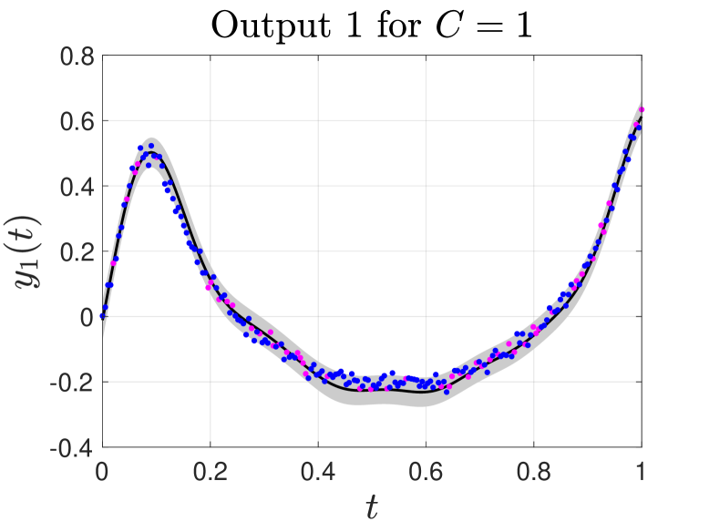
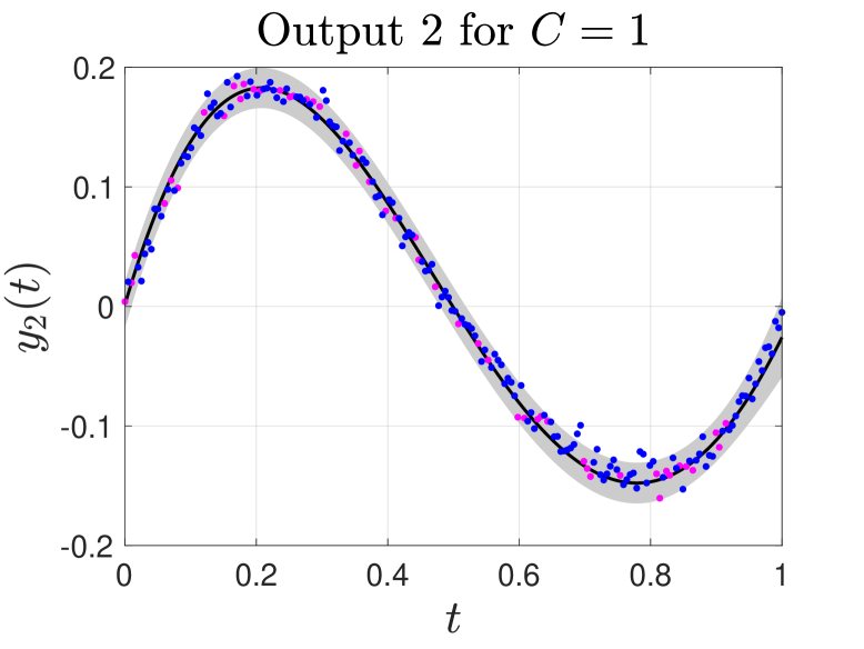
Experimental results are provided for the NCMOGP with homogeneous and separable kernels. In all the experiments that follow, hyperparameter estimation is performed through maximization of the log-marginal likelihood as explained in section 5. We use the normalised mean squared-error (NMSE) and the negative log-predictive density (NLPD) to assess the performance.
Refer to caption
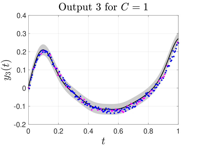
(a) Prediction for y1(t)subscript𝑦1𝑡y_{1}(t) with C=1𝐶1C=1
Refer to caption
(b) Prediction for y2(t)subscript𝑦2𝑡y_{2}(t) with C=1𝐶1C=1
Refer to caption
(c) Prediction for y3(t)subscript𝑦3𝑡y_{3}(t) with C=1𝐶1C=1
Refer to caption
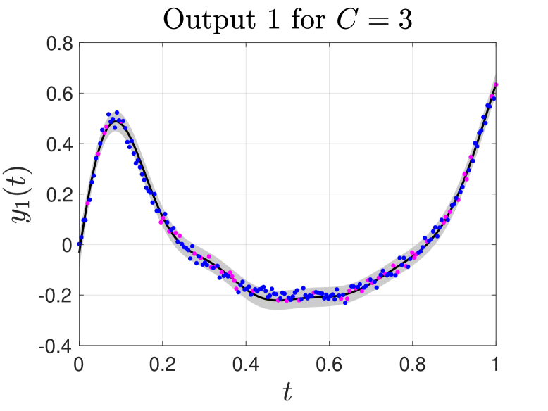
(d) Prediction for y1(t)subscript𝑦1𝑡y_{1}(t) with C=3𝐶3C=3
Refer to caption
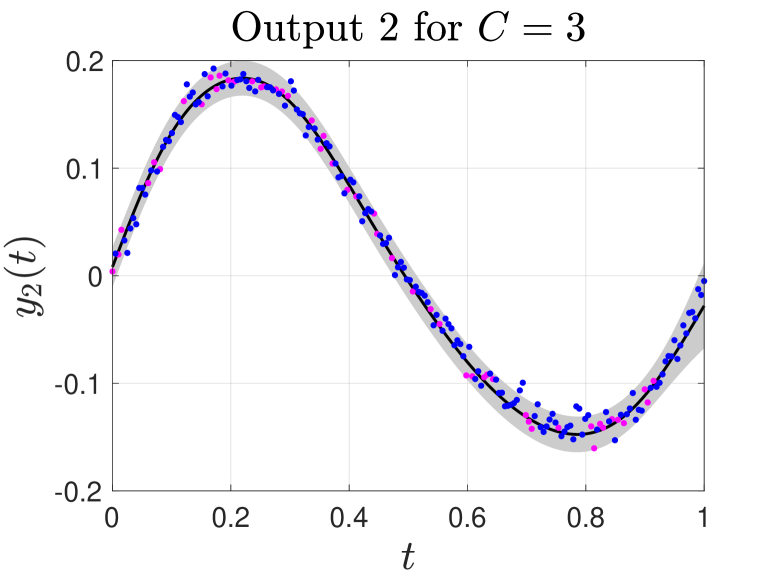
(e) Prediction for y2(t)subscript𝑦2𝑡y_{2}(t) with C=3𝐶3C=3
Refer to caption
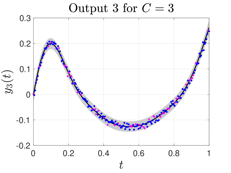
(f) Prediction for y2(t)subscript𝑦2𝑡y_{2}(t) with C=3𝐶3C=3
Figure 1: Comparison of the predictive performance of CMOGP (top row) and NCMOGP with C=3𝐶3C=3 (bottom row) for the dataset synthetically generated. Each column is a different output. Training data is represented using red dots and Test data using blue dots. The black line in the mean over the predictive GP function, and the shaded region denotes two times the standard deviation.

6.1 Toy example

We set a problem of D=3𝐷3D=3 outputs where the smoothing kernels are given as Gd(tτ)=Sdexp(Pd(tτ)2)subscript𝐺𝑑𝑡𝜏subscript𝑆𝑑subscript𝑃𝑑superscript𝑡𝜏2G_{d}(t-\tau)=S_{d}\exp(-P_{d}(t-\tau)^{2}), with parameters S1=5,S2=1,S3=2formulae-sequencesubscript𝑆15formulae-sequencesubscript𝑆21subscript𝑆32S_{1}=5,S_{2}=1,S_{3}=2, and P1=200,P2=0.1formulae-sequencesubscript𝑃1200subscript𝑃20.1P_{1}=200,P_{2}=0.1 and P3=100subscript𝑃3100P_{3}=100. The latent function follows as u(t)=k=14(1k2)cos(2kπt)𝑢𝑡superscriptsubscript𝑘141superscript𝑘22𝑘𝜋𝑡u(t)=\sum_{k=1}^{4}\left(\frac{1}{k^{2}}\right)\cos(2k\pi t). We then numerically solve the convolution integral fd(t)=0tGd(tτ)u(τ)𝑑τsubscript𝑓𝑑𝑡superscriptsubscript0𝑡subscript𝐺𝑑𝑡𝜏𝑢𝜏differential-d𝜏f_{d}(t)=\int_{0}^{t}G_{d}(t-\tau)u(\tau)d\tau for 200200200 datapoints in the input range [0,1]01[0,1]. We compute fd(C=3)(t)=c=13fdc(t)superscriptsubscript𝑓𝑑𝐶3𝑡superscriptsubscript𝑐13superscriptsubscript𝑓𝑑𝑐𝑡f_{d}^{(C=3)}(t)=\sum_{c=1}^{3}f_{d}^{c}(t) and the observed data is obtained by adding Gaussian noise with a variance of σd2=0.005×var[fd(C=3)(t)]superscriptsubscript𝜎𝑑20.005varsuperscriptsubscript𝑓𝑑𝐶3𝑡\sigma_{d}^{2}=0.005\times\operatorname{var}\left[f_{d}^{(C=3)}(t)\right]. We randomly split the dataset into a train set of N=50𝑁50N=50 per output and the rest of the datapoints are used for assessing the performance.

Figure 1 shows qualitative results for predictions made by the CMOGP and a NCMOGP with C=3𝐶3C=3. Although the outputs exhibit a smooth behavior, there are subtle non-linear characteristics that are not captured by the linear model. By zooming in on the interval t[0.4,0.6]𝑡0.40.6t\in[0.4,0.6] for output y1(t)subscript𝑦1𝑡y_{1}(t) (first column in the Figure), we observe that the predictive mean of the linear model (C=1𝐶1C=1) does not completely follow the data compared to the true non-linear model (C=3𝐶3C=3). For output y3(t)subscript𝑦3𝑡y_{3}(t) (third column in the Figure), we observe a similar behavior in the predictive mean of the linear model in the intervals t[0.4,0.8]𝑡0.40.8t\in[0.4,0.8] and t>0.9𝑡0.9t>0.9 compared to the predictive mean of the non-linear model.

Table 1 shows the NMSE and the NLPD for different values of C𝐶C for twenty different partitions of the original dataset into training and testing. We show the average of the metric plus-or-minus a standard deviation. The performance is similar for the non-linear models with C3𝐶3C\geq 3, although the model for C=3𝐶3C=3 shows the lowest standard deviation.

Table 1: Results for the Toy example.
C𝐶C NMSE NLPD
1 0.0142±0.0022plus-or-minus0.01420.00220.0142\pm 0.0022 2.6868±0.0794plus-or-minus2.68680.0794-2.6868\pm 0.0794
2 0.0075±0.0012plus-or-minus0.00750.00120.0075\pm 0.0012 2.9641±0.0665plus-or-minus2.96410.0665-2.9641\pm 0.0665
3 0.0071±0.0009plus-or-minus0.00710.0009\mathbf{0.0071\pm 0.0009} 2.9780±0.0513plus-or-minus2.97800.0513\mathbf{-2.9780\pm 0.0513}
4 0.0072±0.0010plus-or-minus0.00720.00100.0072\pm 0.0010 2.9546±0.0960plus-or-minus2.95460.0960-2.9546\pm 0.0960
5 0.0071±0.0011plus-or-minus0.00710.00110.0071\pm 0.0011 2.9428±0.0956plus-or-minus2.94280.0956-2.9428\pm 0.0956

6.2 Weather data

We use the air temperature dataset considered previously by Nguyen and Bonilla (2014) and used in other multi-output GP papers. The dataset contains air temperature measurements at four spatial locations on the south coast of England: Bramble Bank, Southhampton Dockhead, Chichester Harbour and Chichester Bar, usually refer to by the names Bramblemet, Sotonmet, Cambermet and Chimet, respectively. The measurements correspond to July 10 to July 15, 2013. The prediction problem as introduced in Nguyen and Bonilla (2014) corresponds to predicting consecutive missing data in the outputs Cambermet and Chimet, 173173173 and 201201201 observations, respectively, using observed data from all the stations: 142514251425 observations for Bramblemet, 126812681268 observations for Cambermet, 123512351235 for Chimet and 109710971097 for Sotonmet.

The missing data was artificially removed and we have access to the ground-truth measurements. We compare the non-linear convolution approach to the Intrinsic Coregionalization Model (ICM) (Goovaerts, 1997) and Dependent Gaussian processes (DGP) (Boyle and Frean, 2005). Both models can be seen as particular cases of the non-linear model in Eq. (6). The ICM can be recovered from Eq. (6) by making C=1𝐶1C=1 and Gd,1()=ad,1δ()subscript𝐺𝑑1subscript𝑎𝑑1𝛿G_{d,1}(\cdot)=a_{d,1}\delta(\cdot), where adsubscript𝑎𝑑a_{d} is a scalar that needs to be estimated and δ()𝛿\delta(\cdot) is the Dirac delta function.222Notice that we use a rank one ICM since, similarly to the non-linear model, it only involves one latent function u()𝑢u(\cdot) (Álvarez et al., 2012) DGP is also recovered from (6) assuming C=1𝐶1C=1 and a white-Gaussian process noise model for u()𝑢u(\cdot).

Table 2 reports the mean predictive performance for the missing observations for five random initialisations of the models. CMOGP refers to the NCMOGP with C=1𝐶1C=1. The number at the end of NCMOGP indicates the order C𝐶C of the non-linear model. Results are shown per output with missing data. Notice the reduction in the NMSE for Cambermet for all the non-linear models compared to the linear models (CMOGP and DGP). Here ICM performs better than any of the convolution approaches. For Chimet, there is also a reduction in the NMSE, but only for C=3𝐶3C=3 (NCMOGP3) and C=5𝐶5C=5 (NCMOGP5). In terms of the NLPD, the non-linear model with C=5𝐶5C=5 (NCMOGP5) has a competitive performance when compared to the linear model (CMOGP). The averaged NSMEs for the two outputs are: 0.69890.69890.6989 (C=1𝐶1C=1), 0.57170.57170.5717 (C=2𝐶2C=2), 0.43090.43090.4309 (C=3𝐶3C=3), 0.54560.54560.5456 (C=4𝐶4C=4), 0.47530.47530.4753 (C=5𝐶5C=5), 0.44250.44250.4425 (ICM) and 0.64310.64310.6431 (DGP). The averaged NLPDs for the two ouputs are: 2.06132.06132.0613 (C=1𝐶1C=1), 3.24793.24793.2479 (C=2𝐶2C=2), 2.25502.25502.2550 (C=3𝐶3C=3), 2.54602.54602.5460 (C=4𝐶4C=4), 1.96001.96001.9600 (C=5𝐶5C=5), 2.68482.68482.6848 (ICM) and 1.99251.99251.9925 (DGP). NCMOGP5 offers the best competitive performance both in terms of the NMSE and the NLPD compared to CMOGP, ICM and DGP.

Table 2: Results for the Weather dataset.
Model Cambermet Chimet
NMSE NLPD NMSE NLPD
CMOGP 0.60040.60040.6004 1.98301.98301.9830 0.79740.79740.7974 2.13972.13972.1397
NCMOGP2 0.30800.30800.3080 2.16042.16042.1604 0.83540.83540.8354 4.33554.33554.3355
NCMOGP3 0.43660.43660.4366 2.33332.33332.3333 0.42520.4252\mathbf{0.4252} 2.17662.17662.1766
NCMOGP4 0.26760.26760.2676 2.10752.10752.1075 0.82350.82350.8235 2.98462.98462.9846
NCMOGP5 0.44990.44990.4499 2.09192.09192.0919 0.50070.50070.5007 1.82801.8280\mathbf{1.8280}
ICM 0.10480.1048\mathbf{0.1048} 3.22113.22113.2211 0.78010.78010.7801 2.14852.14852.1485
DGP 0.55130.55130.5513 1.94631.9463\mathbf{1.9463} 0.73490.73490.7349 2.03882.03882.0388

6.3 A high-dimensional input example

The NCMOGP can also be applied for datasets with an input dimension greater than one. We use a subset of the SARCOS dataset333Available at http://www.gaussianprocess.org/gpml/data/ for illustration purposes. The prediction problem corresponds to map from positions, velocities and accelerations to the joint torques in seven degrees-of-freedom SARCOS anthropomorphic robot arm. The datasets contains D=7𝐷7D=7 outputs and the dimension of the input space is p=21𝑝21p=21, corresponding to seven positions, seven velocities, and seven accelerations. The kernels that we use follow the idea described in Section 5 for higher-dimensional inputs.

Our setup is as follows: from the file sarcos_inv.mat we randomly select N=500𝑁500N=500 observations for each output for training and from the file sarcos_inv_test.mat, we randomly select another 500500500 observations for testing. We repeat the experiment ten times for different training and testing sets taken from the same two files.

Table 3: Results for a subset of the SARCOS dataset.
Model NMSE NLPD
CMOGP 0.0497±0.0252plus-or-minus0.04970.02520.0497\pm 0.0252 1.4292±1.1080plus-or-minus1.42921.10801.4292\pm 1.1080
NCMOGP2 0.0478±0.0238plus-or-minus0.04780.02380.0478\pm 0.0238 1.4067±1.1032plus-or-minus1.40671.1032\mathbf{1.4067\pm 1.1032}
NCMOGP3 0.0571±0.0377plus-or-minus0.05710.03770.0571\pm 0.0377 1.4164±1.1401plus-or-minus1.41641.14011.4164\pm 1.1401
NCMOGP4 0.0720±0.0855plus-or-minus0.07200.08550.0720\pm 0.0855 1.4294±1.0787plus-or-minus1.42941.07871.4294\pm 1.0787
NCMOGP5 0.0830±0.0809plus-or-minus0.08300.08090.0830\pm 0.0809 1.4674±1.1449plus-or-minus1.46741.14491.4674\pm 1.1449
ICM 0.0513±0.0246plus-or-minus0.05130.02460.0513\pm 0.0246 1.4208±1.1286plus-or-minus1.42081.12861.4208\pm 1.1286
DGP 0.0477±0.0237plus-or-minus0.04770.0237\mathbf{0.0477\pm 0.0237} 1.4221±1.1088plus-or-minus1.42211.10881.4221\pm 1.1088

Table 3 shows the averaged NMSE and averaged NLPD for the ten repetitions plus-or-minus a standard deviation. The non-linear model NCMOGP2 yields better averaged performance than CMOGP and ICM, in terms of NMSE and a very similar performance to DGP. In terms of NLPD, NCMOGP2 outperforms all the other models, indicating a better performance in terms of the predicted variance. Something to point out is that when looking at the predictive performance for the different NCMOGP, we noticed that each output is usually better predicted by different values of C𝐶C. For example, in terms of NLPD, the best order to predict outputs d=1,2,3,7𝑑1237d=1,2,3,7 would be a non-linear model with C=4𝐶4C=4. The best model for predicting outputs d=4,6𝑑46d=4,6 would be C=3𝐶3C=3, and the best model for predicting output d=5𝑑5d=5 would be C=5𝐶5C=5.

7 CONCLUSIONS AND FUTURE WORK

We have introduced a non-linear extension of the process convolution formalism to build multi-output Gaussian processes. We derived a novel mean function and covariance function from the non-linear operations introduced by the transformations in a Volterra series and showed experimental results that corroborate that these non-linear models have indeed an added benefit in real-world datasets.

We envision several paths for future work. The most pressing one is extending the framework to make it suitable for larger datasets. We can use similar ideas to the ones presented in Moreno-Muñoz et al. (2018) to establish a stochastic variational lower bound for the model introduced in this paper. Exploring the non-linear models for the case of latent force models is also an interesting venue. In this paper we use an smoothing kernel with an EQ form, but it is also possible to use smoothing kernels that correspond to Green’s function of dynamical systems. Automatically learning the smoothing kernel from data is also an alternative as for example in Guarnizo and Álvarez (2017).

An observation from both the Weather and SARCOS experiments, one that could have been expected, is that the predictive performances for the outputs are not all equally good for the same value of C𝐶C. A potential extension of our model would be to allow the automatic learning of the order C𝐶C per output dimension, say Cdsubscript𝐶𝑑C_{d}. Additionally, the kernels we considered were derived assuming that the Volterra kernels were separable and homogeneous. Relaxing both assumptions is yet another path for future research.

References

  • Álvarez and Lawrence [2011] M A Álvarez and N D Lawrence. Computationally efficient convolved multiple output Gaussian processes. Journal of Machine Learning Research, 12:1425–1466, 2011.
  • Álvarez et al. [2012] M A Álvarez, L Rosasco, and N D Lawrence. Kernels for vector-valued functions: A review. Foundations and Trends in Machine Learning, 4(3):195–266, 2012.
  • Álvarez et al. [2013] M A Álvarez, D Luengo, and N D Lawrence. Linear latent force models using Gaussian processes. IEEE Trans. Pattern Anal. Mach. Intell, 35(11):2693–2705, 2013.
  • Barry and Ver Hoef [1996] R P Barry and J M Ver Hoef. Blackbox kriging: spatial prediction without specifying variogram models. Journal of Agricultural, Biological and Environmental Statistics, 1(3):297–322, 1996.
  • Blei et al. [2017] D M Blei, A Kucukelbir, and J D McAuliffe. Variational inference: A review for statisticians. Journal of the American Statistical Association, 112(518):859–877, 2017.
  • Bonilla et al. [2016] E Bonilla, D Steinberg, and A Reid. Extended and unscented kitchen sinks. In International Conference on Machine Learning, pages 1651–1659, 2016.
  • Bonilla et al. [2008] E V Bonilla, K M Chai, and C K I Williams. Multi-task Gaussian process prediction. In NIPS 2007, pages 153–160, 2008.
  • Boyle and Frean [2005] P Boyle and M Frean. Dependent Gaussian processes. In Lawrence Saul, Yair Weiss, and Léon Bouttou, editors, Neural Information Processing Systems, pages 217–224. MIT Press, 2005.
  • Cheng et al. [2017] C M Cheng, Z K Peng, W M Zhang, and G Meng. Volterra-series-based nonlinear system modeling and its engineering applications: A state-of-the-art review. Mechanical Systems and Signal Processing, 87:340–364, 2017.
  • Gallman and Narendra [1976] P G Gallman and K S Narendra. Representations of nonlinear systems via the Stone-Weierstraß theorem. Automatica, 12(6):619–622, 1976.
  • Goovaerts [1997] P Goovaerts. Geostatistics for natural resources evaluation. Oxford University Press, USA, 1997.
  • Guarnizo and Álvarez [2017] C Guarnizo and M A Álvarez. Impulse response estimation of linear time-invariant systems using convolved Gaussian processes and Laguerre functions. In Marcelo Mendoza and Sergio Velastín, editors, CIARP 2017, Valparaiso, Chile, November 7-10, 2017, Proceedings, pages 635–642. Springer International Publishing, 2017.
  • Haber and Keviczky [1999] R Haber and L Keviczky. Nonlinear System Identification – Input-Output Modeling Approach. Kluwer Academic, 1999.
  • Hartikainen and Särkkä [2011] J Hartikainen and S Särkkä. Sequential inference for latent force models. In Proceedings of the Twenty-Seventh Conference on Uncertainty in Artificial Intelligence, UAI’11, pages 311–318. AUAI Press, 2011.
  • Hartikainen et al. [2012] J Hartikainen, M Seppänen, and S Särkkä. State-space inference for non-linear latent force models with application to satellite orbit prediction. In Proceedings of the 29th International Coference on International Conference on Machine Learning, pages 723–730, 2012.
  • Higdon [2002] D M Higdon. Space and space-time modelling using process convolutions. In C. Anderson, V. Barnett, P. Chatwin, and A. El-Shaarawi, editors, Quantitative methods for current environmental issues, pages 37–56, 2002.
  • Lawrence et al. [2007] N D Lawrence, G Sanguinetti, and M Rattray. Modelling transcriptional regulation using Gaussian processes. In Advances in Neural Information Processing Systems, pages 785–792, 2007.
  • Lázaro-Gredilla [2012] M Lázaro-Gredilla. Bayesian warped Gaussian processes. In Advances in Neural Information Processing Systems, pages 1619–1627, 2012.
  • Moreno-Muñoz et al. [2018] P Moreno-Muñoz, A Artés, and M A Álvarez. Heterogeneous multi-output gaussian process prediction. In S. Bengio, H. Wallach, H. Larochelle, K. Grauman, N. Cesa-Bianchi, and R. Garnett, editors, Advances in Neural Information Processing Systems 31, pages 6711–6720. Curran Associates, Inc., 2018.
  • Nguyen and Bonilla [2014] T V Nguyen and E V Bonilla. Collaborative multi-output Gaussian processes. In Proceedings of UAI 2014, Quebec City, Quebec, Canada, pages 643–652, 2014.
  • Rasmussen and Williams [2006] C E Rasmussen and C K I Williams. Gaussian processes for machine learning. MIT Press, 2006.
  • Särkkä [2013] S Särkkä. Bayesian filtering and smoothing, volume 3. Cambridge University Press, 2013.
  • Särkkä et al. [2013] S Särkkä, A Solin, and J Hartikainen. Spatiotemporal learning via infinite-dimensional Bayesian filtering and smoothing: A look at Gaussian process regression through Kalman filtering. IEEE Signal Processing Magazine, 30(4):51–61, 2013.
  • Saul et al. [2016] A D Saul, J Hensman, A Vehtari, and N D Lawrence. Chained Gaussian processes. In Artificial Intelligence and Statistics, pages 1431–1440, 2016.
  • Schetzen [1980] M Schetzen. The Volterra and Wiener theories of nonlinear systems. Wiley, 1980.
  • Song and Lee [2015] I Song and S Lee. Explicit formulae for product moments of multivariate Gaussian random variables. Statistics & Probability Letters, 100:27 – 34, 2015.
  • Steinberg and Bonilla [2014] D M Steinberg and E V Bonilla. Extended and unscented Gaussian processes. In Advances in Neural Information Processing Systems, pages 1251–1259, 2014.
  • Titsias et al. [2009] M K Titsias, N D Lawrence, and M Rattray. Efficient sampling for Gaussian process inference using control variables. In Advances in Neural Information Processing Systems, pages 1681–1688, 2009.
  • Ver Hoef and Barry [1998] J M Ver Hoef and R P Barry. Constructing and fitting models for cokriging and multivariable spatial prediction. Journal of Statistical Plannig and Inference, 69:275–294, 1998.
  • Wills et al. [2013] A Wills, T B Schön, L Ljung, and B Ninness. Identification of Hammerstein–Wiener models. Automatica, 49(1):70–81, 2013.

Supplementary Material

Appendix A LOG LIKELIHOOD

For a given vector of inputs, 𝐭=[tn]n=1N𝐭subscriptsuperscriptdelimited-[]subscript𝑡𝑛𝑁𝑛1\mathbf{t}=[t_{n}]^{N}_{n=1}, the log-marginal likelihood is given as

logp(𝐲|𝐭)=ND2log(2π)12log|𝐊𝐟,𝐟(C)+𝚺12(𝐲𝝁(C))(𝐊𝐟,𝐟(C)+𝚺)1(𝐲𝝁(C)),𝑝conditional𝐲𝐭𝑁𝐷22𝜋conditional12superscriptsubscript𝐊𝐟𝐟𝐶𝚺12superscript𝐲superscript𝝁𝐶topsuperscriptsuperscriptsubscript𝐊𝐟𝐟𝐶𝚺1𝐲superscript𝝁𝐶\displaystyle\log p(\mathbf{y}\,|\,\mathbf{t})=-\frac{ND}{2}\log(2\pi)-\frac{1}{2}\log|\mathbf{K}_{\mathbf{f},\mathbf{f}}^{(C)}+\bm{\Sigma}-\frac{1}{2}(\mathbf{y}-\bm{\mu}^{(C)})^{\top}(\mathbf{K}_{\mathbf{f},\mathbf{f}}^{(C)}+\bm{\Sigma})^{-1}(\mathbf{y}-\bm{\mu}^{(C)}),

where 𝐲=[𝐲1𝐲D]𝐲superscriptdelimited-[]superscriptsubscript𝐲1topsuperscriptsubscript𝐲𝐷toptop\mathbf{y}=[\mathbf{y}_{1}^{\top}\,\ldots\,\mathbf{y}_{D}^{\top}]^{\top} with 𝐲d=[yd(t1)yd(tN)]subscript𝐲𝑑superscriptdelimited-[]subscript𝑦𝑑subscript𝑡1subscript𝑦𝑑subscript𝑡𝑁top\mathbf{y}_{d}=[y_{d}(t_{1})\,\ldots\,y_{d}(t_{N})]^{\top}; 𝝁(C)superscript𝝁𝐶\bm{\mu}^{(C)} and 𝐊𝐟,𝐟(C)superscriptsubscript𝐊𝐟𝐟𝐶\mathbf{K}_{\mathbf{f},\mathbf{f}}^{(C)} have entries given by μd(C)(t)superscriptsubscript𝜇𝑑𝐶𝑡\mu_{d}^{(C)}(t) and kd,d(C)(t,t)superscriptsubscript𝑘𝑑superscript𝑑𝐶𝑡superscript𝑡k_{d,d^{\prime}}^{(C)}(t,t^{\prime}) respectively; and 𝚺𝚺\bm{\Sigma} is the diagonal matrices containing the variances of the noise processes per output. We can find derivatives to this much in the same way as the single output [Rasmussen and Williams, 2006].

Appendix B DERIVATIVES W.R.T. HYPERPARAMETERS

We provide here the derviatives of the mean and covariance functions for the output process with respect to hyperparameters for the purpose of optimisation using a gradient-based method.

Mean Function for Output Process

The mean function for output process is defined

μfd(t)=c=1Cc!2c/2(c2)!(kd,d(t,t))c/2subscript𝜇subscript𝑓𝑑𝑡subscriptsuperscript𝐶𝑐1𝑐superscript2𝑐2𝑐2superscriptsubscript𝑘𝑑𝑑𝑡𝑡𝑐2\displaystyle\mu_{f_{d}}(t)=\sum^{C}_{c=1}\frac{c!}{2^{c/2}\left(\frac{c}{2}\right)!}\left(k_{d,d}(t,t)\right)^{c/2}

and its derivative with respect to the kernel hyperparameters θdsuperscript𝜃𝑑\theta^{d} is

μfd(t)θd=c=1Cc!2(c/2)(c2)!(c2)(kd,d(t,t))(c/2)1kd,d(t,t)θd.subscript𝜇subscript𝑓𝑑𝑡subscript𝜃𝑑subscriptsuperscript𝐶𝑐1𝑐superscript2𝑐2𝑐2𝑐2superscriptsubscript𝑘𝑑𝑑𝑡𝑡𝑐21subscript𝑘𝑑𝑑𝑡𝑡superscript𝜃𝑑\displaystyle\frac{\partial\mu_{f_{d}}(t)}{\partial\theta_{d}}=\sum^{C}_{c=1}\frac{c!}{2^{(c/2)}\left(\frac{c}{2}\right)!}\left(\frac{c}{2}\right)\left(k_{d,d}(t,t)\right)^{(c/2)-1}\frac{\partial k_{d,d}(t,t)}{\partial\theta^{d}}.

Covariance Function for Output Process

We define the covariance function of the output process as

kyd,yd(t,t)=subscript𝑘subscript𝑦𝑑subscript𝑦superscript𝑑𝑡superscript𝑡absent\displaystyle k_{y_{d},y_{d^{\prime}}}(t,t^{\prime})= c=1Cc=1C𝐋T𝐚Ac,c,𝐋((kd,d(t,t))l11(kd,d(t,t))l12(kd,d(t,t))l22)subscriptsuperscript𝐶𝑐1subscriptsuperscript𝐶superscript𝑐1subscript𝐋subscript𝑇𝐚subscript𝐴𝑐superscript𝑐𝐋superscriptsubscript𝑘𝑑𝑑𝑡𝑡subscript𝑙11superscriptsubscript𝑘𝑑superscript𝑑𝑡superscript𝑡subscript𝑙12superscriptsubscript𝑘superscript𝑑superscript𝑑superscript𝑡superscript𝑡subscript𝑙22\displaystyle\sum^{C}_{c=1}\sum^{C}_{c^{\prime}=1}\sum_{\mathbf{L}\in T_{\mathbf{a}}}A_{c,c^{\prime},\mathbf{L}}\bigg{(}(k_{d,d}(t,t))^{l_{11}}(k_{d,d^{\prime}}(t,t^{\prime}))^{l_{12}}(k_{d^{\prime},d^{\prime}}(t^{\prime},t^{\prime}))^{l_{22}}\bigg{)}
(c=1Cc!2c/2(c2)!(kd,d(t,t))c/2)(c=1Cc!2c/2(c2)!(kd,d(t,t))c/2),subscriptsuperscript𝐶𝑐1𝑐superscript2𝑐2𝑐2superscriptsubscript𝑘𝑑𝑑𝑡𝑡𝑐2subscriptsuperscript𝐶superscript𝑐1superscript𝑐superscript2superscript𝑐2superscript𝑐2superscriptsubscript𝑘superscript𝑑superscript𝑑superscript𝑡superscript𝑡superscript𝑐2\displaystyle\quad-\Bigg{(}\sum^{C}_{c=1}\frac{c!}{2^{c/2}\left(\frac{c}{2}\right)!}(k_{d,d}(t,t))^{c/2}\Bigg{)}\Bigg{(}\sum^{C}_{c^{\prime}=1}\frac{c^{\prime}!}{2^{c^{\prime}/2}\left(\frac{c^{\prime}}{2}\right)!}(k_{d^{\prime},d^{\prime}}(t^{\prime},t^{\prime}))^{c^{\prime}/2}\Bigg{)},

where

Ac,c,𝐋=c!c!2l11+l22l11!l12!l22!.subscript𝐴𝑐superscript𝑐𝐋𝑐superscript𝑐superscript2subscript𝑙11subscript𝑙22subscript𝑙11subscript𝑙12subscript𝑙22\displaystyle A_{c,c^{\prime},\mathbf{L}}=\frac{c!c^{\prime}!}{2^{l_{11}+l_{22}}l_{11}!l_{12}!l_{22}!}.

The derivative with respect to θdsubscript𝜃𝑑\theta_{d} is therefore

kyd,yd(t,t)θd=subscript𝑘subscript𝑦𝑑subscript𝑦superscript𝑑𝑡superscript𝑡superscript𝜃𝑑absent\displaystyle\frac{\partial k_{y_{d},y_{d^{\prime}}}(t,t^{\prime})}{\partial\theta^{d}}= c=1Cc=1C𝐋T𝐚Ac,c,𝐋(l11(kd,d(t,t))l111(kd,d(t,t))l12(kd,d(t,t))l22kd,d(t,t)θd)\displaystyle\sum^{C}_{c=1}\sum^{C}_{c=1}\sum_{\mathbf{L}\in T_{\mathbf{a}}}A_{c,c^{\prime},\mathbf{L}}\Bigg{(}l_{11}(k_{d,d}(t,t))^{l_{11}-1}(k_{d,d^{\prime}}(t,^{\prime}t))^{l_{12}}(k_{d^{\prime},d^{\prime}}(t^{\prime},t^{\prime}))^{l_{22}}\frac{\partial k_{d,d}(t,t)}{\partial\theta^{d}}\Bigg{)}
+(l12(kd,d(t,t))l11(kd,d(t,t))l121(kd,d(t,t))l22kd,d(t,t)θd)\displaystyle\quad+\Bigg{(}l_{12}(k_{d,d}(t,t))^{l_{11}}(k_{d,d^{\prime}}(t,^{\prime}t))^{l_{12}-1}(k_{d^{\prime},d^{\prime}}(t^{\prime},t^{\prime}))^{l_{22}}\frac{\partial k_{d,d^{\prime}}(t,t^{\prime})}{\partial\theta^{d}}\Bigg{)}
(c=1Cc!2c/2(c2)!(c2)(kd,d(t,t))(c/2)1kd,d(t,t)θd)(c=1Cc!2c/2(c2)!(kd,d(t,t))c/2).subscriptsuperscript𝐶𝑐1𝑐superscript2𝑐2𝑐2𝑐2superscriptsubscript𝑘𝑑𝑑𝑡superscript𝑡𝑐21subscript𝑘𝑑𝑑𝑡𝑡superscript𝜃𝑑subscriptsuperscript𝐶superscript𝑐1superscript𝑐superscript2superscript𝑐2superscript𝑐2superscriptsubscript𝑘superscript𝑑superscript𝑑superscript𝑡superscript𝑡superscript𝑐2\displaystyle\quad-\Bigg{(}\sum^{C}_{c=1}\frac{c!}{2^{c/2}\left(\frac{c}{2}\right)!}\left(\frac{c}{2}\right)(k_{d,d}(t,t^{\prime}))^{(c/2)-1}\frac{\partial k_{d,d}(t,t)}{\partial\theta^{d}}\Bigg{)}\Bigg{(}\sum^{C}_{c^{\prime}=1}\frac{c^{\prime}!}{2^{c^{\prime}/2}\left(\frac{c^{\prime}}{2}\right)!}(k_{d^{\prime},d^{\prime}}(t^{\prime},t^{\prime}))^{c^{\prime}/2}\Bigg{)}.